Econ 240C

Lecture 16

2

Part I. VAR

• Does the Federal Funds Rate Affect Capacity Utilization?

3

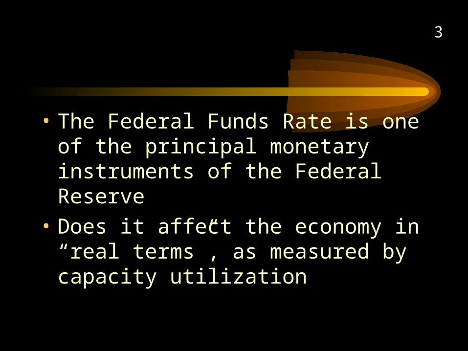
• The Federal Funds Rate is one of the principal monetary instruments of the Federal Reserve

• Does it affect the economy in “real terms”, as measured by capacity utilization

4

Preliminary Analysis

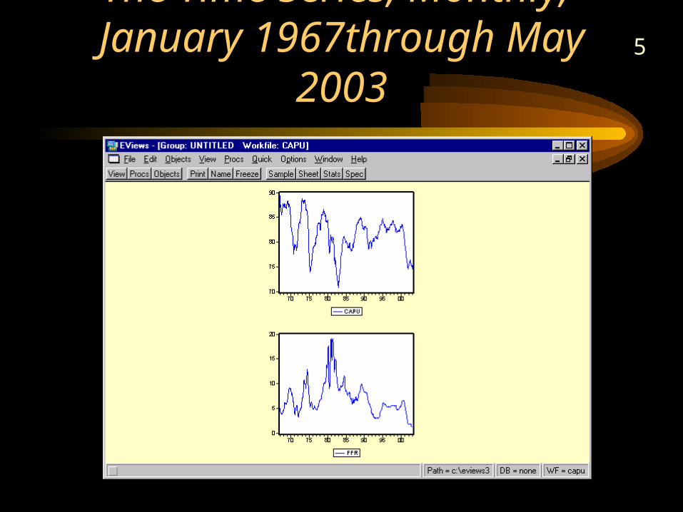
5The Time Series, Monthly, January 1967through May 2003

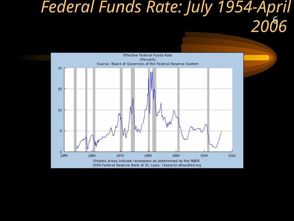
6Federal Funds Rate: July 1954-April 2006

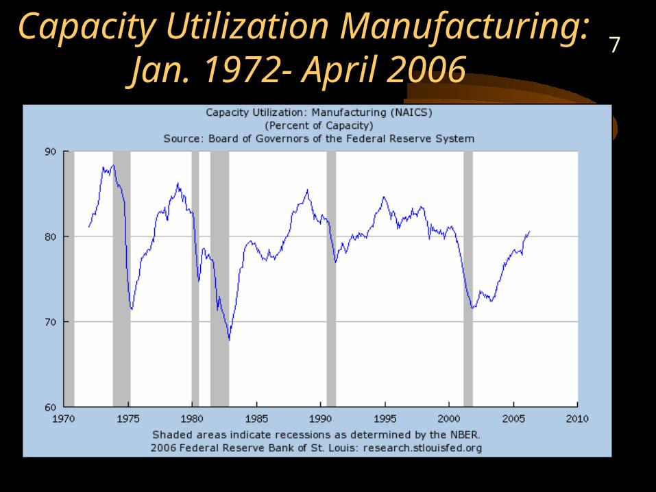
7Capacity Utilization Manufacturing:

Jan. 1972- April 2006

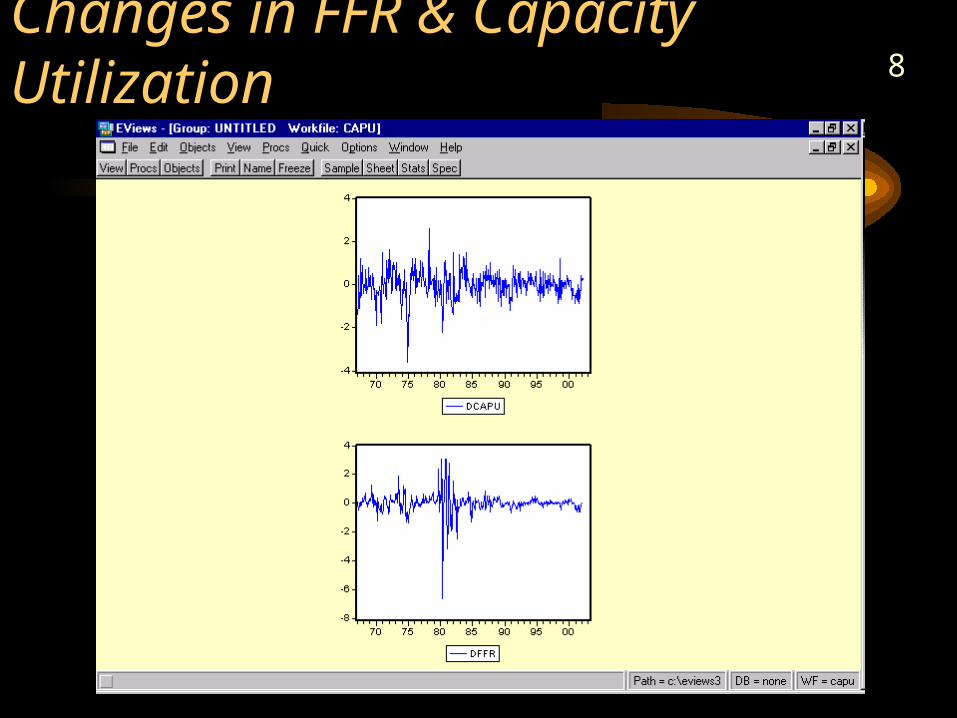
8Changes in FFR & Capacity Utilization

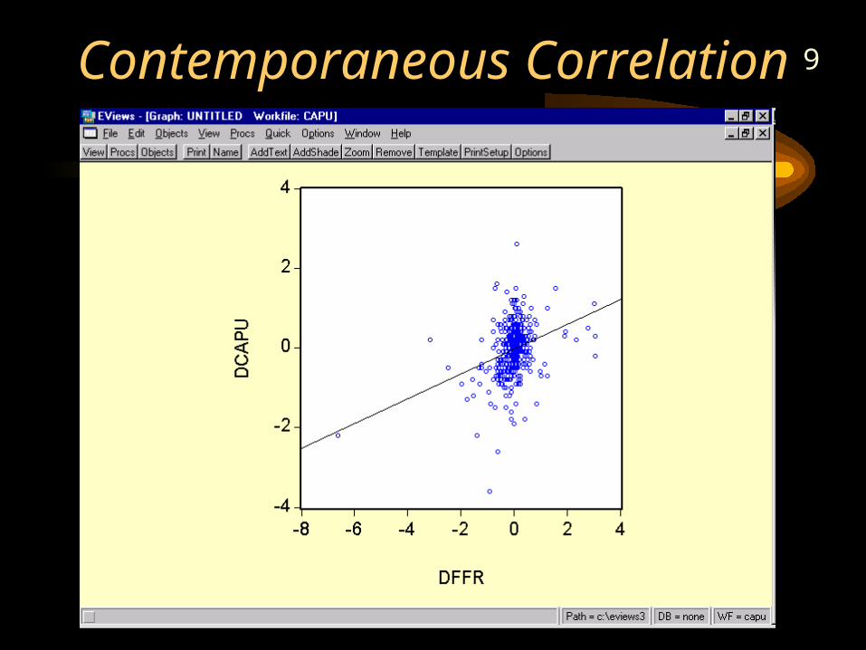
9Contemporaneous Correlation

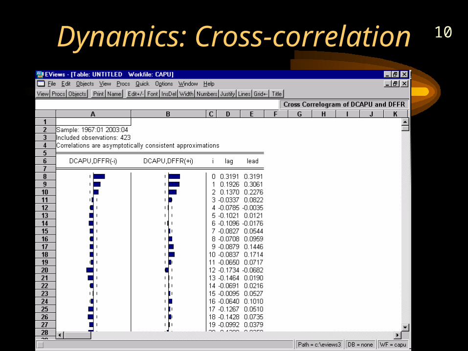
10Dynamics: Cross-correlation

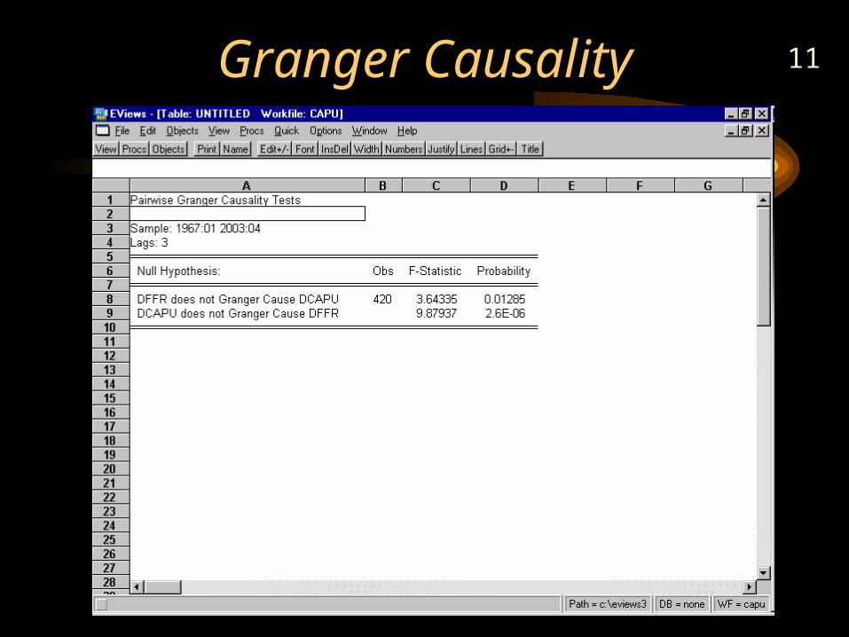
11Granger Causality

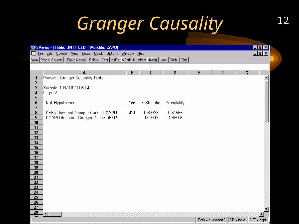
12Granger Causality

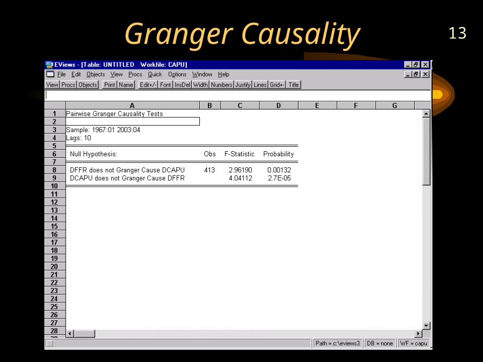
13Granger Causality

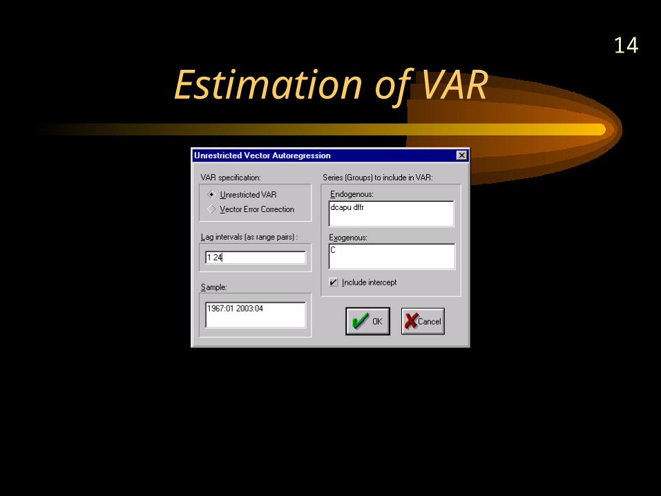
14

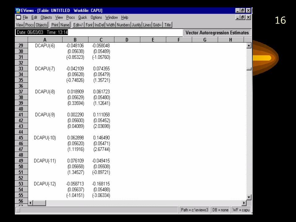
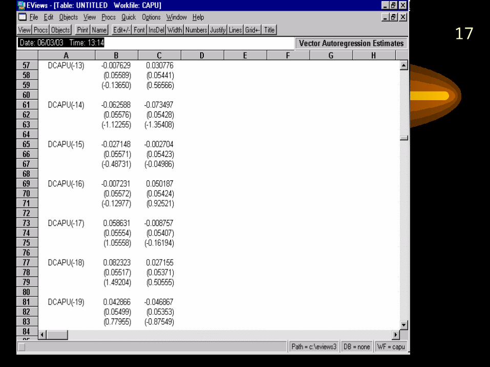
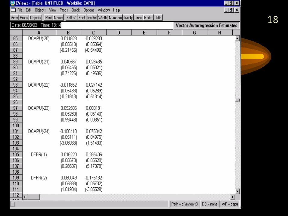
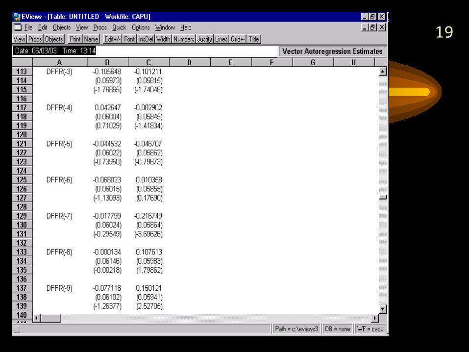
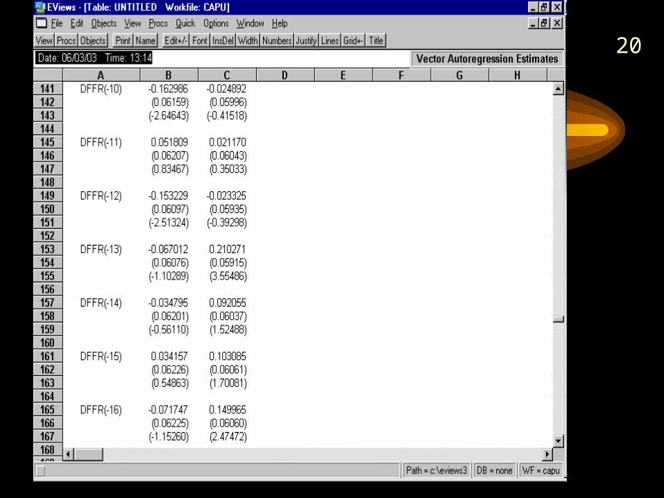
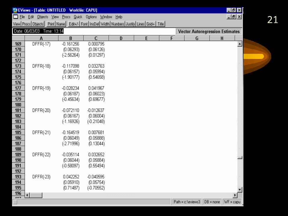
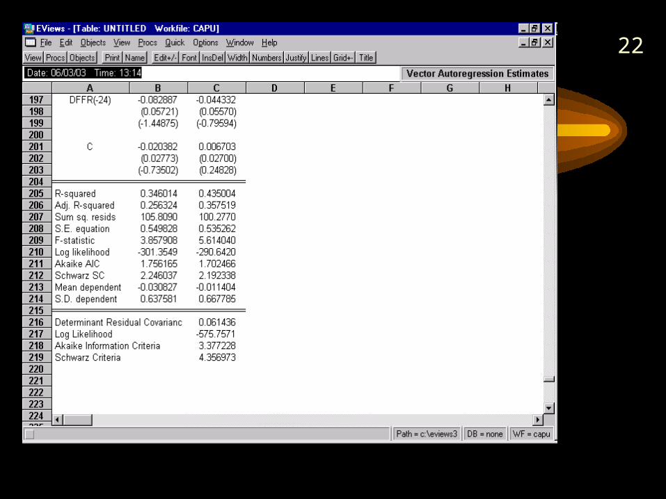
Estimation of VAR

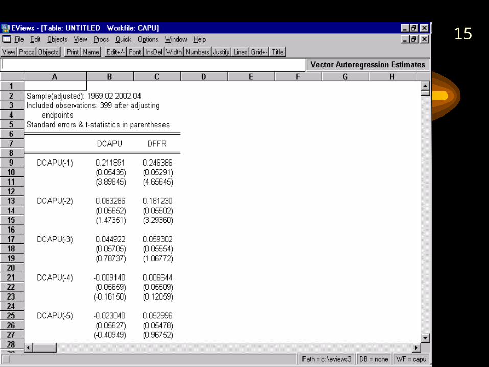
15

16

17

18

19

20

21

22

23

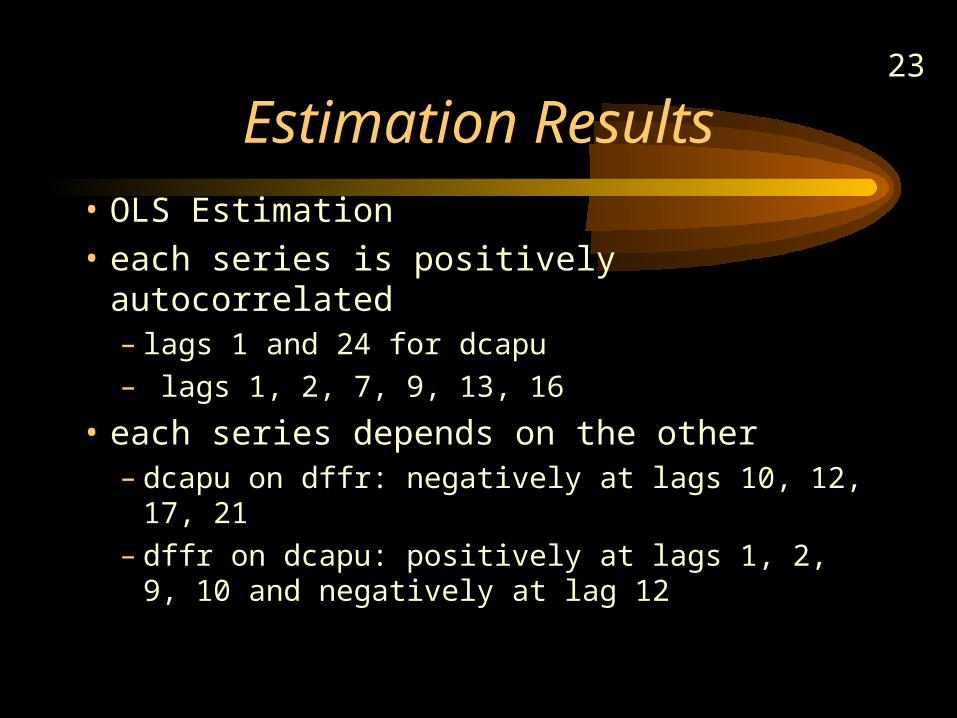
Estimation Results

• OLS Estimation

• each series is positively autocorrelated– lags 1 and 24 for dcapu– lags 1, 2, 7, 9, 13, 16

• each series depends on the other– dcapu on dffr: negatively at lags 10, 12, 17, 21– dffr on dcapu: positively at lags 1, 2, 9, 10 and

negatively at lag 12

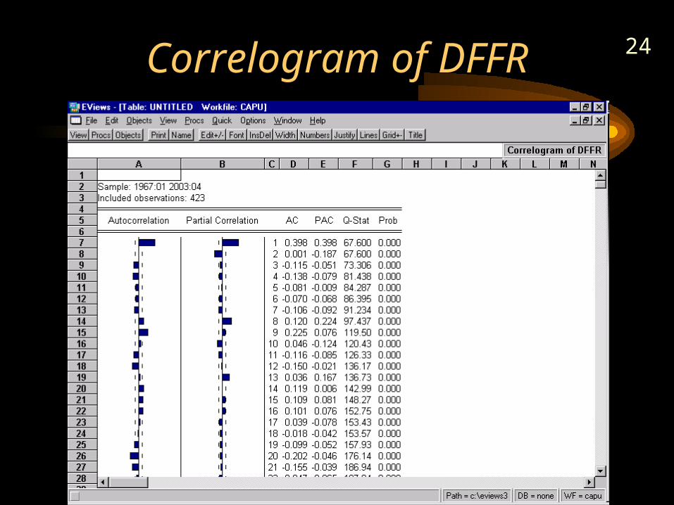
24Correlogram of DFFR

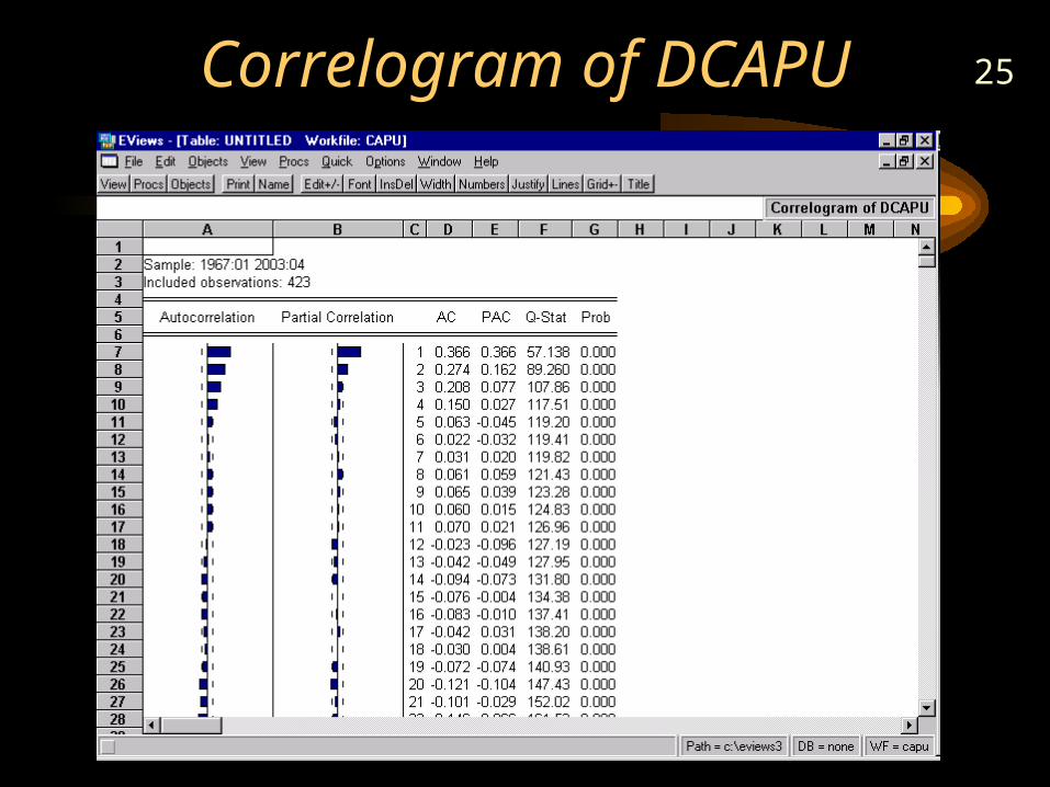
25Correlogram of DCAPU

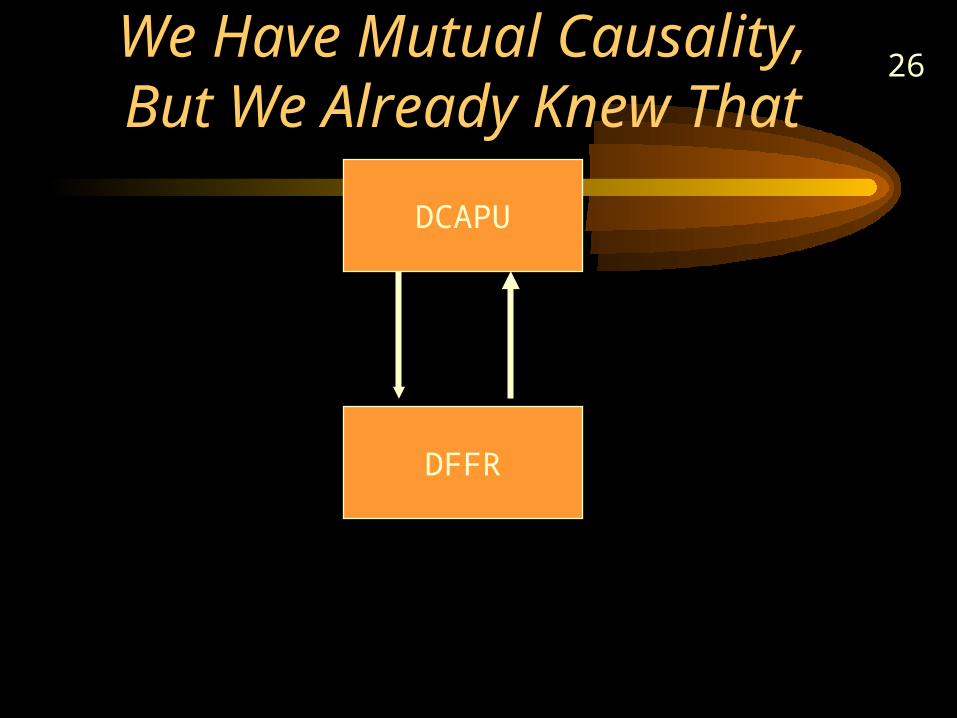
26We Have Mutual Causality, But

We Already Knew That

DCAPU

DFFR

27

Interpretation

• We need help

• Rely on assumptions

28

What If

• What if there were a pure shock to dcapu– as in the primitive VAR, a shock that only

affects dcapu immediately

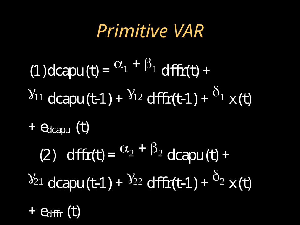
Primitive VAR

(1)dcapu(t) = dffr(t) +

dcapu(t-1) + dffr(t-1) + x(t)

+ edcapu(t)

(2) dffr(t) = dcapu(t) +

dcapu(t-1) + dffr(t-1) + x(t)

+ edffr(t)

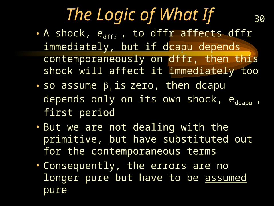
30The Logic of What If• A shock, edffr , to dffr affects dffr immediately,

but if dcapu depends contemporaneously on dffr, then this shock will affect it immediately too

• so assume is zero, then dcapu depends only on its own shock, edcapu , first period

• But we are not dealing with the primitive, but have substituted out for the contemporaneous terms

• Consequently, the errors are no longer pure but have to be assumed pure

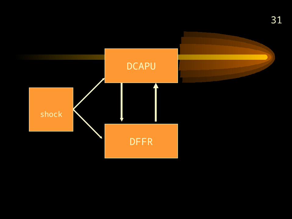
31

DCAPU

DFFR

shock

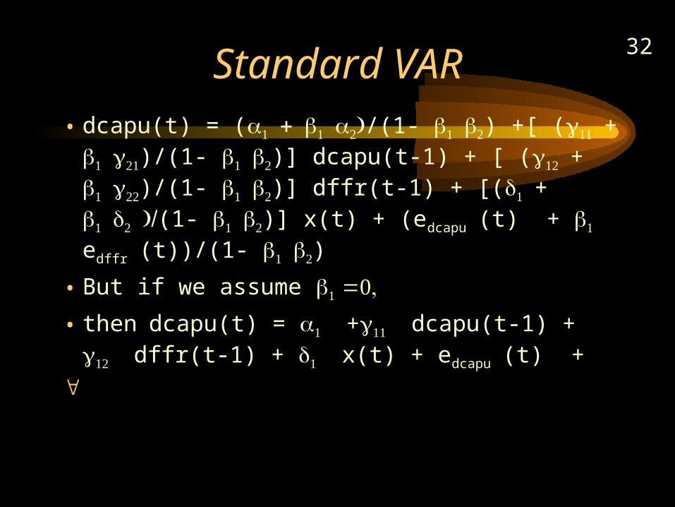
32Standard VAR

• dcapu(t) = (/(1- ) +[ (+ )/(1- )] dcapu(t-1) + [ (+ )/(1- )] dffr(t-1) + [(+ (1- )] x(t) + (edcapu(t) + edffr(t))/(1- )

• But if we assume

• thendcapu(t) = + dcapu(t-1) + dffr(t-1) + x(t) + edcapu(t) +

33

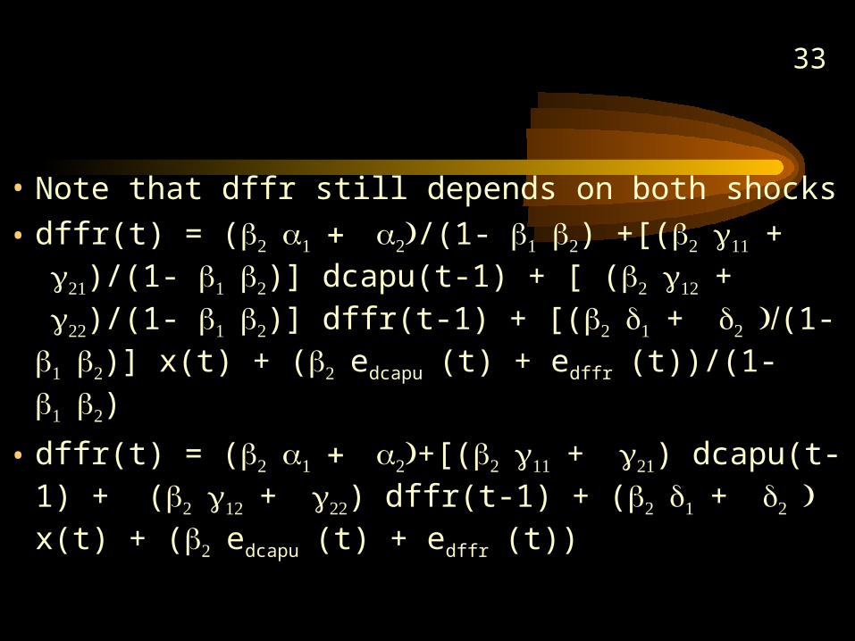
• Note that dffr still depends on both shocks

• dffr(t) = (/(1- ) +[(+ )/(1- )] dcapu(t-1) + [ (+ )/(1- )] dffr(t-1) + [(+ (1- )] x(t) + (edcapu(t) + edffr(t))/(1- )

• dffr(t) = (+[(+ ) dcapu(t-1) + (+ ) dffr(t-1) + (+ x(t) + (edcapu(t) + edffr(t))

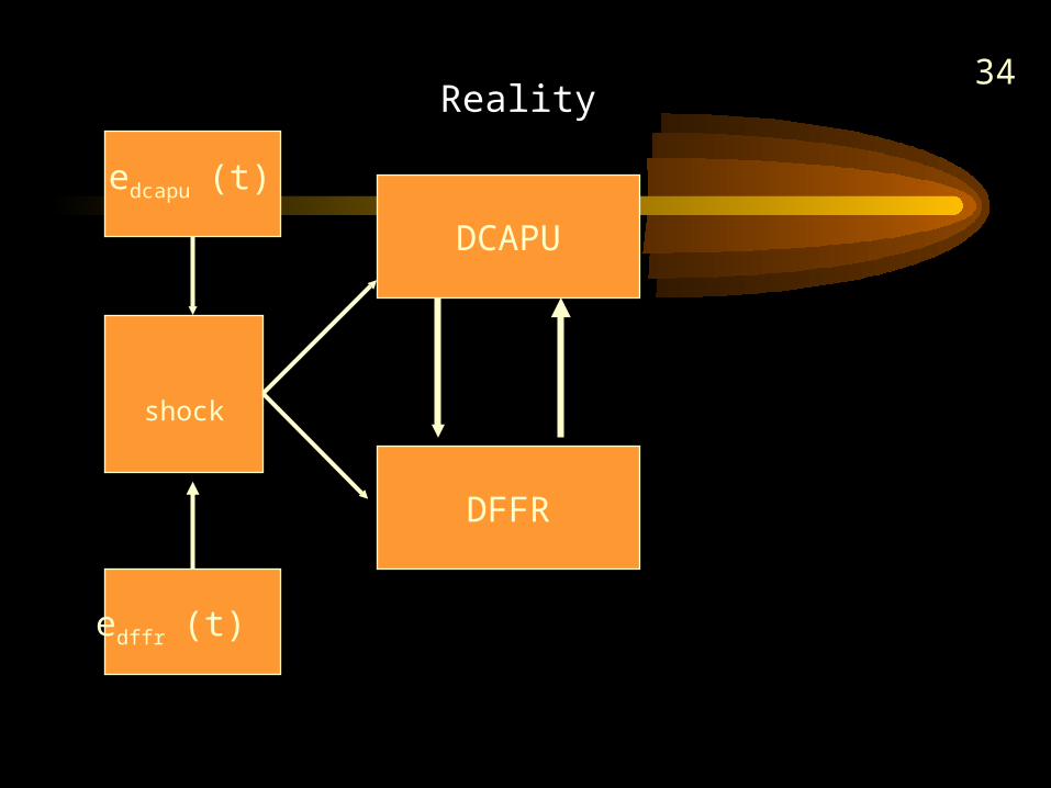
34

DCAPU

DFFR

shock

edcapu(t)

edffr(t)

Reality

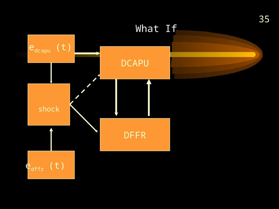
35

DCAPU

DFFR

shock

edcapu(t)

edffr(t)

What If

36EVIEWS

37

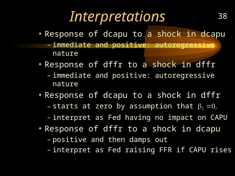
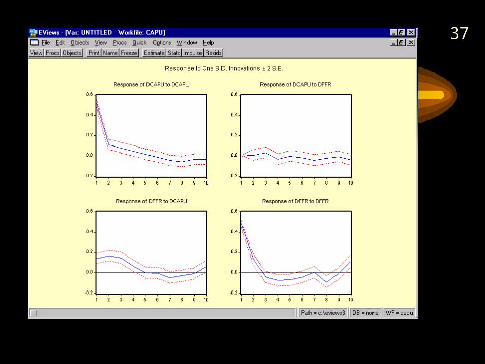
38Interpretations• Response of dcapu to a shock in dcapu

– immediate and positive: autoregressive nature

• Response of dffr to a shock in dffr– immediate and positive: autoregressive nature

• Response of dcapu to a shock in dffr– starts at zero by assumption that – interpret as Fed having no impact on CAPU

• Response of dffr to a shock in dcapu– positive and then damps out– interpret as Fed raising FFR if CAPU rises

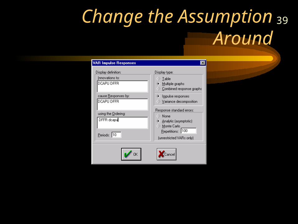
39

Change the Assumption Around

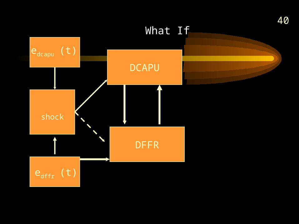
40

DCAPU

DFFR

shock

edcapu(t)

edffr(t)

What If

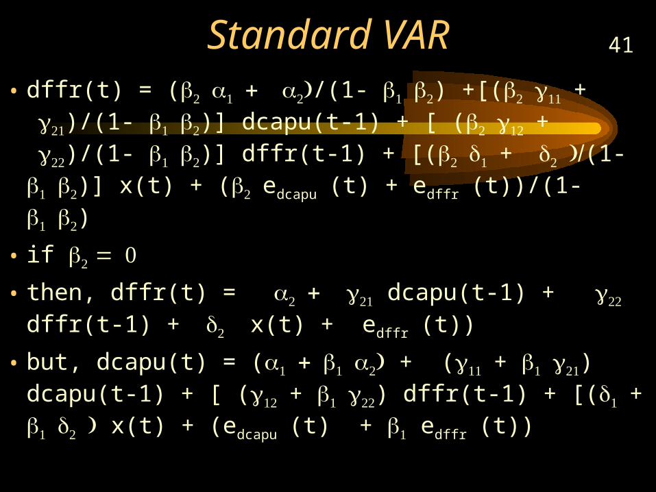
41Standard VAR• dffr(t) = (/(1- ) +[(+ )/(1-

)] dcapu(t-1) + [ (+ )/(1- )] dffr(t-1) + [(+ (1- )] x(t) + (edcapu(t) + edffr(t))/(1- )

• if

• then, dffr(t) = dcapu(t-1) + dffr(t-1) + x(t) + edffr(t))

• but, dcapu(t) = ( + (+ ) dcapu(t-1) + [ (+ ) dffr(t-1) + [(+ x(t) + (edcapu(t) + edffr(t))

42

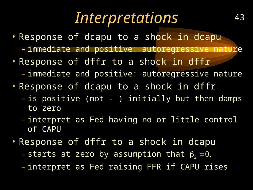
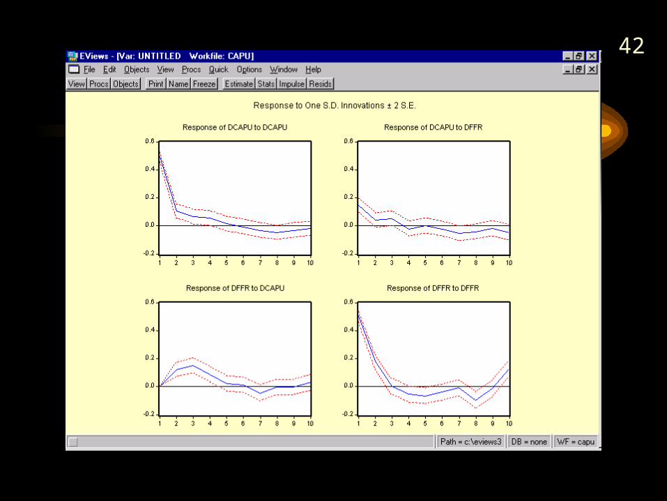
43Interpretations• Response of dcapu to a shock in dcapu

– immediate and positive: autoregressive nature

• Response of dffr to a shock in dffr– immediate and positive: autoregressive nature

• Response of dcapu to a shock in dffr– is positive (not - ) initially but then damps to zero– interpret as Fed having no or little control of CAPU

• Response of dffr to a shock in dcapu– starts at zero by assumption that – interpret as Fed raising FFR if CAPU rises

44Conclusions• We come to the same model interpretation

and policy conclusions no matter what the ordering, i.e. no matter which assumption we use, or

• So, accept the analysis

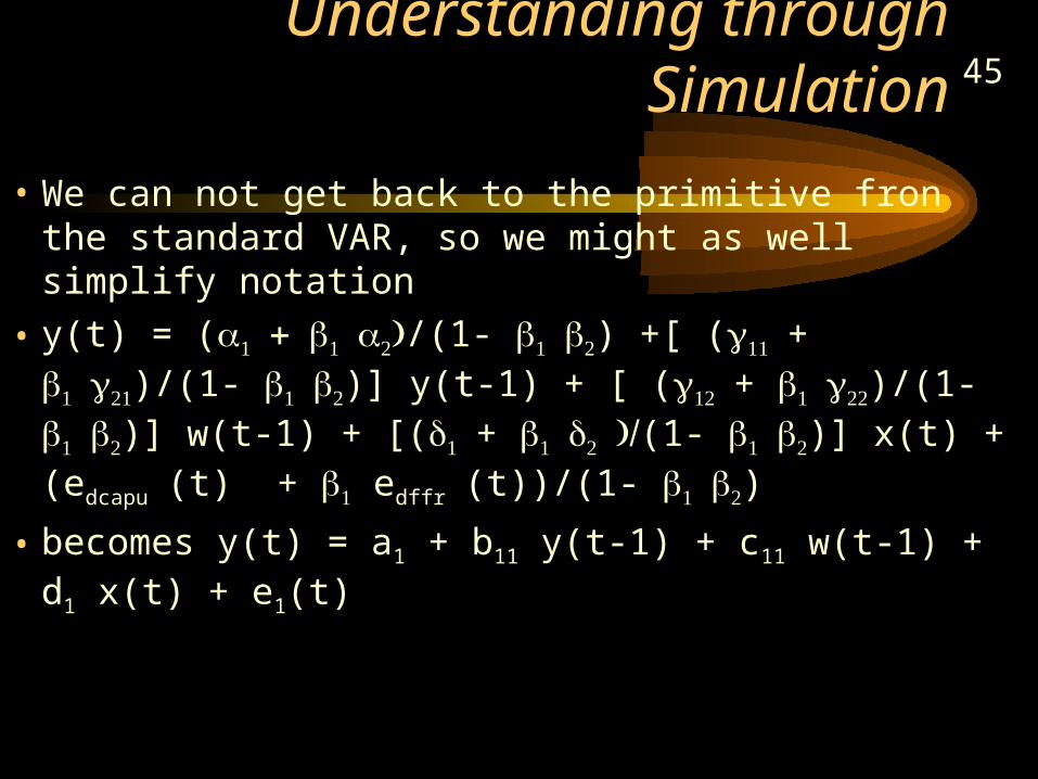
45Understanding through Simulation

• We can not get back to the primitive fron the standard VAR, so we might as well simplify notation

• y(t) = (/(1- ) +[ (+ )/(1- )] y(t-1) + [ (+ )/(1- )] w(t-1) + [(+ (1- )] x(t) + (edcapu(t) + edffr(t))/(1- )

• becomes y(t) = a1 + b11 y(t-1) + c11 w(t-1) + d1 x(t) + e1(t)

46

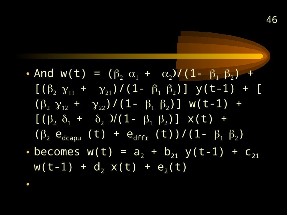
• And w(t) = (/(1- ) +[(+ )/(1- )] y(t-1) + [ (+ )/(1- )] w(t-1) + [(+ (1- )] x(t) + (edcapu(t) + edffr(t))/(1- )

• becomes w(t) = a2 + b21 y(t-1) + c21 w(t-1) + d2 x(t) + e2(t)

•

47

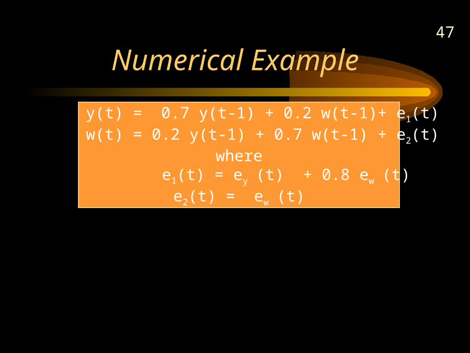
Numerical Example

y(t) = 0.7 y(t-1) + 0.2 w(t-1)+ e1(t)w(t) = 0.2 y(t-1) + 0.7 w(t-1) + e2(t)

where e1(t) = ey(t) + 0.8 ew(t)

e2(t) = ew(t)

48

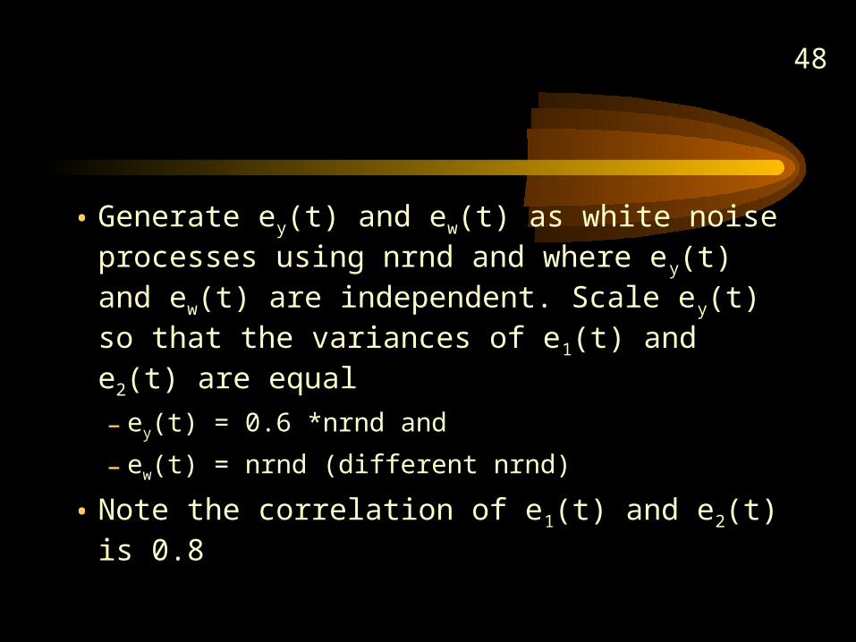
• Generate ey(t) and ew(t) as white noise processes using nrnd and where ey(t) and ew(t) are independent. Scale ey(t) so that the variances of e1(t) and e2(t) are equal

– ey(t) = 0.6 *nrnd and

– ew(t) = nrnd (different nrnd)

• Note the correlation of e1(t) and e2(t) is 0.8

49

Analytical Solution Is Possible

• These numerical equations for y(t) and w(t) could be solved for y(t) as a distributed lag of e1(t) and a distributed lag of e2(t), or, equivalently, as a distributed lag of ey(t) and a distributed lag of ew(t)

• However, this is an example where simulation is easier

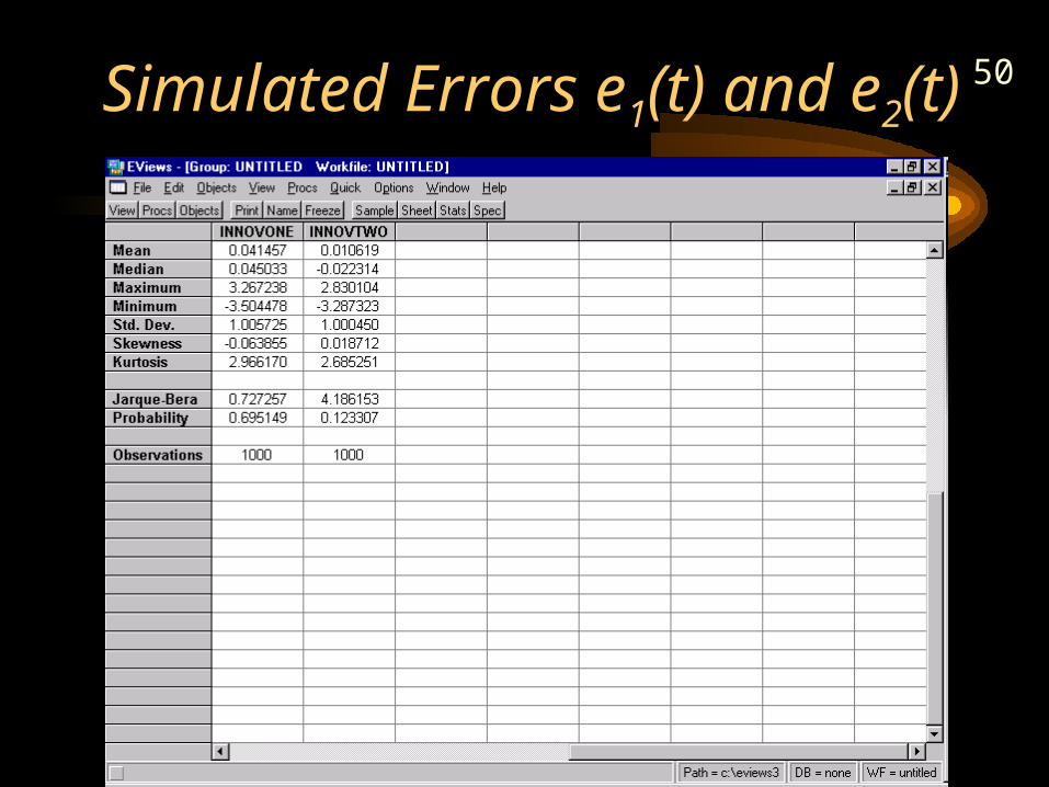
50Simulated Errors e1(t) and e2(t)

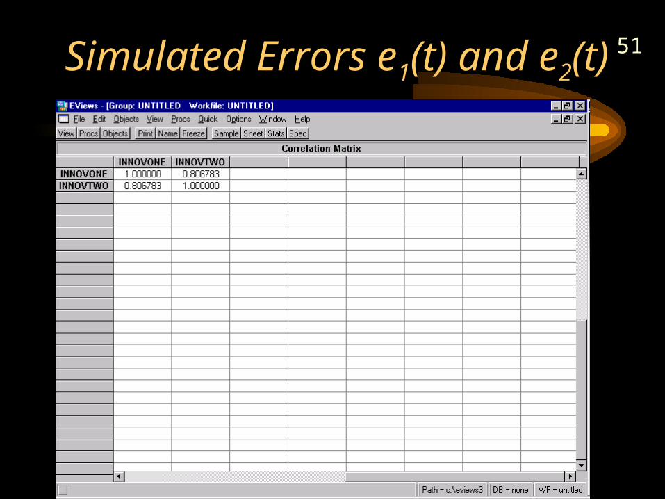
51Simulated Errors e1(t) and e2(t)

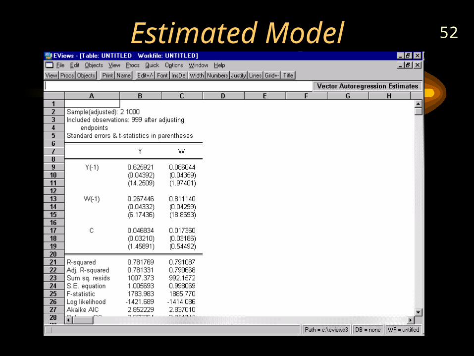
52Estimated Model

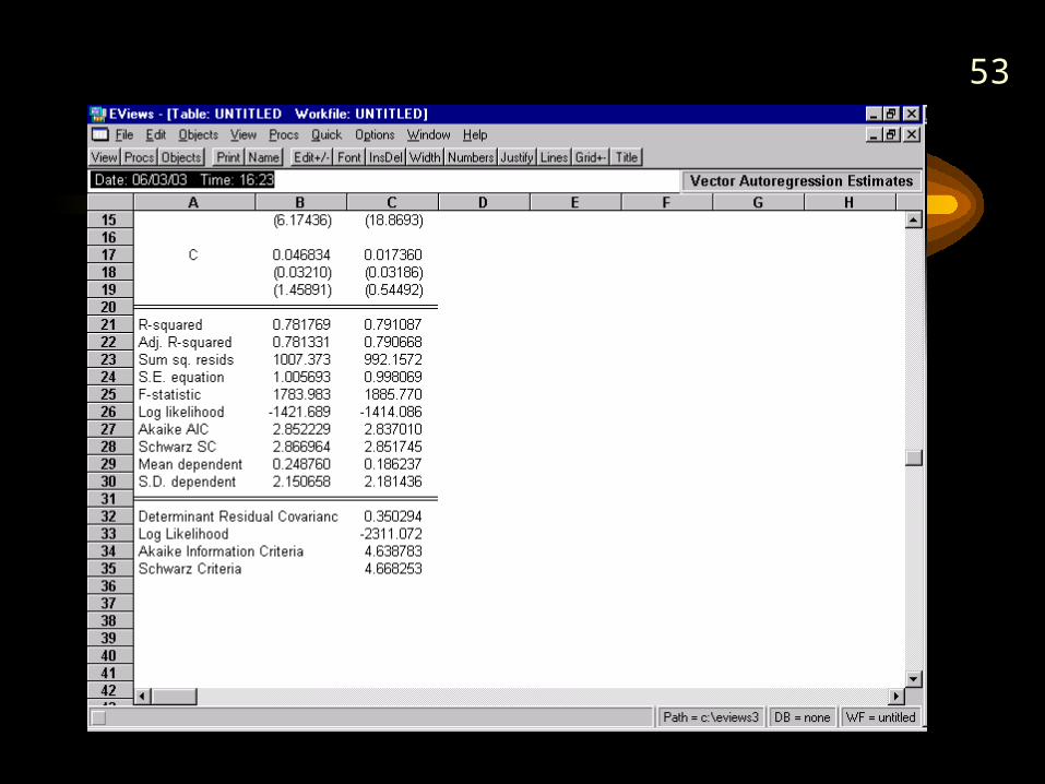
53

54

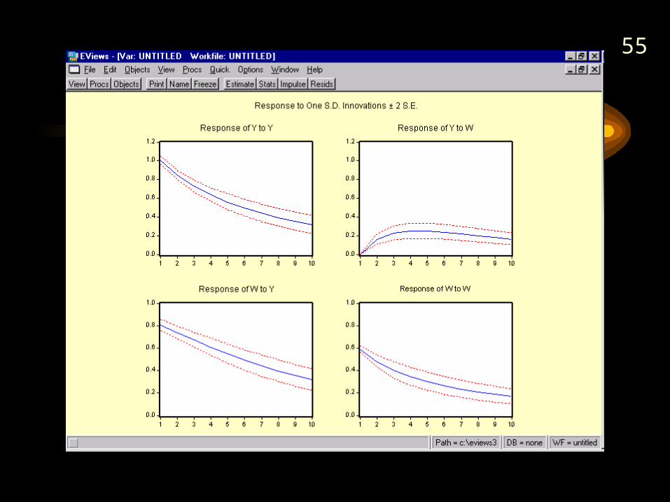
55

56

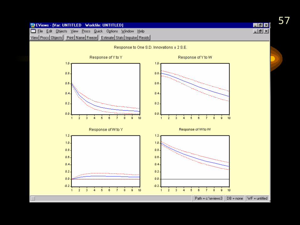
57

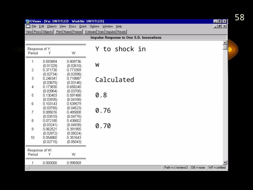
58

Y to shock in w

Calculated

0.8

0.76

0.70

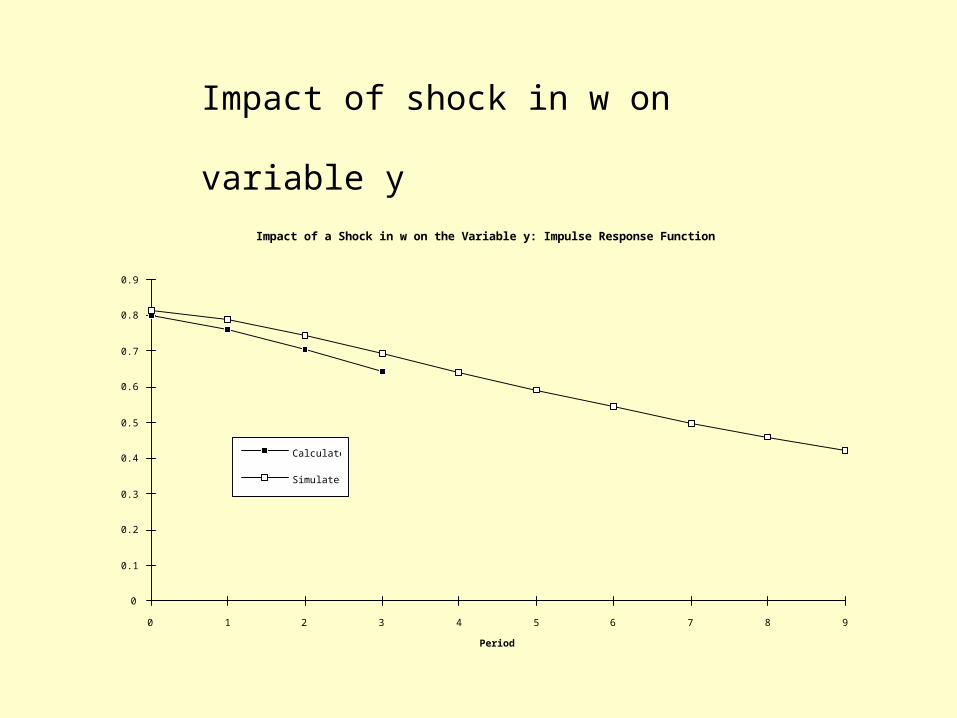
Impact of a Shock in w on the Variable y: Impulse Response Function

Period

Imp

act

Mult

iplier

0

0.1

0.2

0.3

0.4

0.5

0.6

0.7

0.8

0.9

0 1 2 3 4 5 6 7 8 9

Calculated

Simulated

Impact of shock in w on variable y

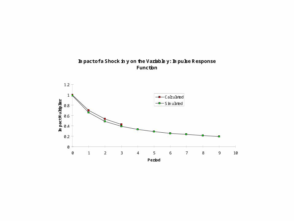
Impact of a Shock in y on the Variable y: Impulse Response Function

0

0.2

0.4

0.6

0.8

1

1.2

0 1 2 3 4 5 6 7 8 9 10

Period

Impac

t M

ultip

lier

Calculated

Simulated