Embed Size (px)
Citation preview

ECONOMETRIC ANALYSIS OF 15-MINUTE INTRADAY ELECTRICITY PRICES
RÜDIGER KIESEL FLORENTINA PARASCHIV WORKING PAPERS ON FINANCE NO. 2015/21 INSTITUTE OF OPERATIONS RESEARCH AND COMPUTATIONAL FINANCE
(IOR/CF – HSG)
OCTOBER 2015

Electronic copy available at: http://ssrn.com/abstract=2671379
Econometric analysis of 15-minute intraday
electricity prices
Rudiger Kiesela,∗, Florentina Paraschivb,∗∗
aChair for Energy Finance, University of Duisburg-Essen, Universitatsstrasse 12,D-45117 Essen, Germany
bInstitute for Operations Research and Computational Finance,University of St. Gallen, Bodanstrasse 6, CH-9000, St. Gallen, Switzerland
Abstract
The trading activity in the German intraday electricity market has increasedsignificantly over the last years. This is partially due to an increasing shareof renewable energy, wind and photovoltaic, which requires power generatorsto balance out the forecasting errors in their production. We investigate thebidding behaviour in the intraday market by looking at both last prices andcontinuous bidding, in the context of a fundamental model. A unique dataset of 15-minute intraday prices and intraday-updated forecasts of wind andphotovoltaic has been employed and price bids are modelled by prior informa-tion on fundamentals. We show that intraday prices adjust asymmetrically toboth forecasting errors in renewables and to the volume of trades dependenton the threshold variable demand quote, which reflects the expected demandcovered by the planned traditional capacity in the day-ahead market. Thelocation of the threshold can be used by market participants to adjust theirbids accordingly, given the latest updates in the wind and photovoltaic fore-casting errors and the forecasts of the control area balances.
Keywords: intraday electricity prices, bidding behavior, renewable energy,forecasting model
∗Part of the work was done while the author was visiting Center of Advanced Study,Norwegian Academy of Sciences and Letters, Oslo, as a member of the group: Stochasticsfor Environmental and Financial Economics
∗∗Corresponding author: Florentina Paraschiv, [email protected]; Part ofthe work has been done during my visiting terms at the University of Duisburg-Essen,funded by the Chair for Energy Trading and Finance.
Preprint submitted to Elsevier October 8, 2015

Electronic copy available at: http://ssrn.com/abstract=2671379
1. Introduction1
Trading in the intraday electricity markets increased rapidly since the2
opening of the market. This may be driven by the need of photovoltaic and3
wind power operators to balance their production forecast errors, i.e. de-4
viations between forecasted and actual production. Evidence for this is a5
jump in the volume of intraday trading as the direct marketing of renewable6
energy was introduced. Furthermore, there may be a generally increased in-7
terest in intraday trading activities due to proprietary trading. We study the8
structure of intraday trading of electricity and identify the price-driving fac-9
tors. Our main goal is to identify market fundamental factors that influence10
the bidding behavior in the 15-minute intraday market at European Power11
Exchange (EPEX).12
Along the basic timeline of electricity trading activities, see Figure 1, the13
intraday activities relate mostly to further adjustments of positions after the14
closure of the day-ahead market.15
Figure 1: Timing Electricity Trading
While day-ahead trading offers the possibility to correct long-term pro-16
duction schedule (build on the forward markets) in terms of hourly produc-17
tion schedule of power plants (Delta Hedging) and to adjust for residual load18
profiles on an hourly basis, the increasing share of renewable energy sources19
(wind, solar) in electricity markets requires a finer adjustment.20
According to the Equalization Mechanism Ordinance (ger.: Verordnung21
zur Weiterentwicklung des bundesweiten Ausgleichsmechanismus, abbr.:22
2

AuglMechV) all electricity generated by renewable sources has to be traded23
day-ahead. This is usually done by the transmission system operator (TSO)24
with the plant operator receiving a legally guaranteed feed-in-tariff. From25
2012 on the inclusion of a market premium led direct marketers within the26
feed-in premium support scheme to enter the market as well. Trading of elec-27
tricity from a renewable energy source is based on forecasts which may have28
a horizon of up to 36 h (taking some data-handling into account). To correct29
errors in forecasts the AusglMechV requires the marketers of renewable en-30
ergy to use the intraday market to balance differences in actual and updated31
forecasts. Intraday trading starts at 3 pm and takes place continuously until32
up to 45 min (by 2015 this was shortened to 30 min) before the start of the33
traded quarter-hour. As forecasts change regularly, marketers may sell and34
buy the same contract at different times during the trading period.35
After the closure of the intraday market balancing energy has to be used36
to close differences between available and forecasted electricity. As a smaller37
number of power plants are used for balancing energy the merit-order curve38
is steeper than that in the intraday market. Thus on average larger prices39
are paid and marketers aim at minimising this difference, see [5]. In addition,40
TSOs may impose sanctions on marketers who frequently require balancing41
energy.42
Balancing energy is supplied by generators with the necessary flexibility to43
balance the market. In case generation is below demand positive balancing44
energy is used, otherwise negative balancing energy. [6] and [13] contain45
a detailed description of the integration of renewable energy in electricity46
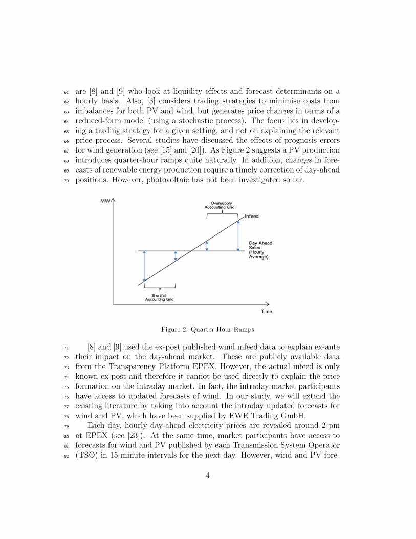
markets and the regulatory requirements and we refer the reader to these47
sources for further information.48
The day-ahead market (spot market) and the balancing markets have49
been investigated extensively. For example, ([22]) show that the day-ahead50
price formation process at EPEX depends on the interaction/substitution51
effect between the traditional production capacity (coal, gas, oil) with the52
fluctuant renewable energies (wind and photovoltaic (PV)). Further empirical53
studies on intraday/balancing markets include [1], [16]. Also, [18] studies54
strategic behaviour linking day-ahead and balancing markets.55
An investigation in the merit-order effect is given by [2], wo find that56
electricity generation by wind and PV has reduced spot market prices con-57
siderably by 6 e/MWh in 2010 rising to 10 e/MWh in 2012. They also show58
that merit order effects are projected to reach 14-16 e/MWh in 2016.59
Recent studies of the intraday high-frequency electricity prices at EPEX60
3
are [8] and [9] who look at liquidity effects and forecast determinants on a61
hourly basis. Also, [3] considers trading strategies to minimise costs from62
imbalances for both PV and wind, but generates price changes in terms of a63
reduced-form model (using a stochastic process). The focus lies in develop-64
ing a trading strategy for a given setting, and not on explaining the relevant65
price process. Several studies have discussed the effects of prognosis errors66
for wind generation (see [15] and [20]). As Figure 2 suggests a PV production67
introduces quarter-hour ramps quite naturally. In addition, changes in fore-68
casts of renewable energy production require a timely correction of day-ahead69
positions. However, photovoltaic has not been investigated so far.70
Figure 2: Quarter Hour Ramps
[8] and [9] used the ex-post published wind infeed data to explain ex-ante71
their impact on the day-ahead market. These are publicly available data72
from the Transparency Platform EPEX. However, the actual infeed is only73
known ex-post and therefore it cannot be used directly to explain the price74
formation on the intraday market. In fact, the intraday market participants75
have access to updated forecasts of wind. In our study, we will extend the76
existing literature by taking into account the intraday updated forecasts for77
wind and PV, which have been supplied by EWE Trading GmbH.78
Each day, hourly day-ahead electricity prices are revealed around 2 pm79
at EPEX (see [23]). At the same time, market participants have access to80
forecasts for wind and PV published by each Transmission System Operator81
(TSO) in 15-minute intervals for the next day. However, wind and PV fore-82
4

casts are updated frequently during the trading period. Thus, at the time83
when market participants place their bids for a particular intraday delivery84
period (hour, quarter of hour), updated information about the forecasting85
errors of renewables becomes available. In consequence, also deviations be-86
tween the intraday prices and the day-ahead price for a specific hour are87
expected to occur. Our main research question is, thus, to which extent do88
market participants change their bidding behavior when new information on89
wind and PV forecasts becomes available. We will employ a unique data set90
of the latest forecasts of wind and PV available at the time of the bid.91
Our analysis is twofold: Firstly, we derive an asymmetric fundamental92
model for the difference between the last price bid for a certain quarter93
of hour and the day-ahead price for that hour. We distinguish between94
summer/winter, peak/off-peak hours. We test for asymmetric behavior of95
prices to forecasting errors of renewable energy dependent on the demand96
quote regime and further investigate the typical jigsaw pattern of intraday97
prices. Thus, we identify a seasonality shape that provides traders important98
information about the time of the day when they can bid, dependent on their99
demand/supply profiles. Furthermore, the effect of volume of trades/market100
liquidity are investigated. Secondly, we are interested in the bidding behavior101
of market participants in the intraday electricity market, continuous bidding.102
We thus analyse the continuous trades and disentangle the effect of market103
fundamentals dependent on the time of the day. The econometric model is104
replicated for several traded hourly quarters, in different time of the day.105
In particular, we are interested to see how delta bid prices change when106
new information becomes available in the intraday renewable forecasts for107
wind and PV. We look at the trade-off between autoregressive terms and108
fundamental factors impacting the intraday price formation process.109
Our contribution to the existing literature is twofold: we use ex-ante fore-110
casts of fundamental variables and employ high-frequency, namely quarter-111
hourly intraday prices.112
2. Model architecture113
Our main assumption is that the electricity intraday price formation pro-114
cess depends on how much traditional capacity has been allocated in the115
day-ahead market and in which proportion it covers the forecasted demand.116
Let us consider two possible market regimes:117
5

1. The traditional capacity planned for the day-ahead satisfies the ex-118
pected demand for a certain hour;119
2. There is a certain demand quote uncovered by the planned capacity.120
Thus, in scenario 2, negative forecasting errors of wind and PV will increase121
faster the intraday prices than in scenario 1, due to the excess demand pres-122
sure. Viceversa, in scenario 1, positive forecasting errors in renewables will123
put pressure on traditional suppliers to reduce the production, since renew-124
ables are fed into the grid with priority (on average 20% of electricity pro-125
duction in Germany is wind and PV based). Thus, prices will decrease faster126
than in scenario 2, where the excess of renewables (positive updated fore-127
casts) will balance out the excess demand. Therefore, in the context of a128
threshold model, we investigate whether there is an asymmetric adjustment129
of the intraday prices to forecasting errors in renewables, dependent on the130
demand quote regime (proportion of the forecasted demand for electricity131
in the planned traditional capacity for the day-ahead). The location of the132
threshold in the demand quote is estimated and this gives an indication of the133
bidding behavior in the intraday market. Market participants can compare134
the identified threshold value to the forecasted demand quote for a certain135
hour to identify the market regime and to further define a bidding strategy.136
Employing the demand quote as threshold variable is supported by the lit-137
erature as several papers have found that total electricity demand influences138
price behaviour strongly. In [14] it is shown that the ratio between wind and139
conventional power production affects the electricity price most (the so-called140
wind penetration). [19] identify the residual load, the electricity demand that141
needs to be met by conventional power, as an important variable.142
To include trading volume as a fundamental variable is also supported143
by the literature as e.g. [6] find that the forecast balancing costs in intraday144
trading are linked to the trading volume. This is in line with earlier papers ,145
such as [17] and [4], who estimate asymmetric GARCH models and include146
traded electricity volume in the variance equation to study its impact on147
price volatility.148
In a first part of our analysis we aim at a model for the difference between149
the last intraday bid price for a certain quarter of an hour and the day-ahead150
price for that specific hour. As a prerequisite for our modeling approach, we151
investigate the typical jigsaw pattern of the 15-minute intraday prices and152
control for seasonality. Figures 3, 4, 5 show the long-term mean of last prices153
6

and average prices bid for a certain quarter of an hour between 01/01/2014–154
01/07/2014. During the day, the jigsaw pattern is mainly explained by the155
following situation: Renewable energy providers sell day-ahead the full hour156
(average of all quarters). During morning (evening) hours the sun goes up157
(down) so in the first quarter there is a buy-pressure on them as they are158
not able to produce the hourly average. On the other hand, in the fourth159
quarter they produce too much and have to sell.160
We also found a persistent jigsaw pattern of prices during off-peak hours.161
This is driven by the production design of fossil power plants (supply side:162
when it starts low and ends high) or power-intensive industry (demand side:163
when it starts high and ends low).164
A reason for that my be inter-temporal restrictions in using fossil plants.165
In addition to fuel costs, these plants have ramp-up and ramp-down costs,166
which prevent plant operators from shutting down plants in case of drops in167
demand or starting up plants in case of spikes in demand. The short-term168
marginal costs from this may dominate fuel costs.169
3. Data170
As motivated in section 2, for the analysis we employed historical day-171
ahead and intraday electricity prices for 15-minute products in the continuous172
trading system between 01/01/2014–30/06/2014. As fundamental variables173
selected in this study we refer to demand forecast, power plant availability,174
intraday updated forecasts for wind and photovoltaic, volume trades in the175
continuous trading, and the control area balance. The latter represents the176
corresponding use of balancing power in the balancing market1. In partic-177
ular, the control area balance corresponds to the sum of all balance group178
deviations of balance groups registered at the transmission system operator179
and of the relevant balance groups owned by the transmission system oper-180
ator (e.g. EEG, grid losses, unintentional deviation)2. In Tables 1 and 2 we181
give an overview of the data sources and their frequency, respectively.182
1As balance group deviations are not immediately available online the control areabalance is calculated on the basis of the corresponding use of balancing power. Thepublished data are values from operating measurements that are adjusted by measurementcorrections if necessary. The actual settlement-relevant data can be retrieved under theprices for grid balancing.
2see http://www.tennettso.de
7

0
50
100
150
200
250
0
10
20
30
40
50
60
70
0 153045 0 153045 0 153045 0 153045 0 153045 0 153045 0 153045 0 153045 0 153045 0 153045 0 153045 0 153045
8 9 10 11 12 13 14 15 16 17 18 19
Sun
shin
e D
ura
tio
n
EUR
/MW
h
Intraday quarter-hourly prices long-term mean summer
Price_Last_Avg
Mean_Price_Avg
Sunshine_Avg
0
200
400
600
800
1000
1200
1400
1600
1800
2000
0
10
20
30
40
50
60
70
0 153045 0 153045 0 153045 0 153045 0 153045 0 153045 0 153045 0 153045 0 153045 0 153045 0 153045 0 153045
8 9 10 11 12 13 14 15 16 17 18 19
Vo
lum
e Tr
ades
EUR
/MW
h
Intraday quarter-hourly prices long-term mean summer
Price_Last_Avg
Sunshine_Avg
SumVol_Avg
Figure 3: Seasonality pattern of the last prices and average prices bid for a certainquarter of an hour during the peak hours in summer. The right axes show thesunshine duration and the sum of volumes traded.
8

0
10
20
30
40
50
60
70
80
90
0
10
20
30
40
50
60
70
80
0 153045 0 153045 0 153045 0 153045 0 153045 0 153045 0 153045 0 153045 0 153045 0 153045 0 153045 0 153045
8 9 10 11 12 13 14 15 16 17 18 19
Sun
shin
e D
ura
tio
n
EUR
/MW
h
Intra-day quarter-hourly prices long-term mean winter
Price_Last_Avg
Mean_Price_Avg
Sunshine_Avg
0
200
400
600
800
1000
1200
1400
0
10
20
30
40
50
60
70
80
0 153045 0 153045 0 153045 0 153045 0 153045 0 153045 0 153045 0 153045 0 153045 0 153045 0 153045 0 153045
8 9 10 11 12 13 14 15 16 17 18 19
Vo
lum
e T
rad
es
EUR
/MW
h
Intra-day quarter-hourly prices long-term mean winter
Price_Last_Avg
Mean_Price_Avg
SumVol_Avg
Figure 4: Seasonality pattern of the last prices and average prices bid for a certainquarter of an hour during the peak hours in winter. The right axes show thesunshine duration and the sum of volumes traded.
9

0
200
400
600
800
1000
1200
1400
0
10
20
30
40
50
60
70
0 153045 0 153045 0 153045 0 153045 0 153045 0 153045 0 153045 0 153045 0 153045 0 153045 0 153045 0 153045
20 21 22 23 0 1 2 3 4 5 6 7
Sum
Vo
lum
e A
vera
ge
Pri
ces
Long-term mean intraday quarter-hourly prices offpeak summer
Price_Last_Avg
Mean_Price_Avg
SumVol_Avg
0
200
400
600
800
1000
1200
0
10
20
30
40
50
60
70
0 153045 0 153045 0 153045 0 153045 0 153045 0 153045 0 153045 0 153045 0 153045 0 153045 0 153045 0 153045
20 21 22 23 0 1 2 3 4 5 6 7
Sum
Vo
lum
e A
vera
ge
Pri
ces
Long-term mean intraday quarter-hourly prices offpeak winter
Price_Last_Avg
Mean_Price_Avg
SumVol_Avg
Figure 5: Seasonality pattern of the last prices and average prices bid for a certainquarter of an hour during the off-peak hours in summer and winter, respectively.The right axis shows the sum of volumes traded.
10

Variableunits
Description Data Source
Day-ahead PriceEUR/MWh
Market clearing price for a cer-tain hour in the day-ahead auc-tions (Phelix)
European Power Exchange (EPEX)https://www.epexspot.com/en/
Intraday PriceEUR/MWh
Intraday electricity prices for15-minute products in the con-tinuous trading
European Energy Exchange Trans-parency Platform:http://www.eex-transparency.com/de
Intraday VolumeTradesMWh
Intraday volume trades for 15-minute products in the contin-uous trading
European Energy Exchange Trans-parency Platform:http://www.eex-transparency.com/de
Wind ForecastMW
Sum of intraday forecasted in-feed of wind electricity into thegrid
EWE TRADING GmbHhttp://www.ewe.com/en/
PV ForecastMW
Sum of intraday forecasted in-feed of PV electricity into thegrid
EWE TRADING GmbHhttp://www.ewe.com/en/
Expected PowerPlant AvailabilityMW
Ex-ante expected power plantavailability for electricity pro-duction on the delivery day(daily granularity), daily pub-lished at 10:00 am
European Energy Exchange& transmission system operators:ftp://infoproducts.eex.com
Expected DemandMW
Demand forecast for the rele-vant hour on the delivery day
European Network of TransmissionSystem Operators (ENTSOE):https://transparency.entsoe.eu/
Control area bal-anceMW
Balancing market margins,available ex-post for a certaindelivery period
Transmission system operators:http://www.50Hertz.com,http://www.amprion.de,http://www.transnetbw.de,http://www.tennettso.de
Table 1: Overview of fundamental variables used in the analysis
Variable Daily Hourly quarter-hourly
Day-ahead Price ×Intraday Price ×Intraday Volume Trades ×Wind Forecast ×PV Forecast ×Expected Power Plant Availability ×Expected Demand ×Control area balance ×
Table 2: Data granularity of fundamental variables
4. Methodology183
4.1. Threshold model specification184
The technical specification of our model follows [21] and reads:185
yi = θ′
1xi + εi, ωi ≤ τ, (1)
11

yi = θ′
2xi + εi, ωi > τ, (2)
where ωi is the threshold variable used to split the sample into two regimes.186
The random variable εi is a regression error.187
Our observed sample is yi, xi, ωini=1, where yi represent the dependent188
variable and xi is an m-vector of independent variables. The threshold vari-189
able ωi may be an element of xi and is assumed to have a continuous dis-190
tribution. To write the model in a single equation3, we define the dummy191
variable di(τ) = 1[ωi ≤ τ ], where 1[·] is the indicator function and we set192
xi(τ) := xidi(τ). Furthermore, let λ′n = θ
′2 − θ
′1 denote the threshold effect.193
Thus, equations (1) and (2) become:194
yi = θ′xi + λ′nxi(τ) + εi (3)
In order to simplify the threshold estimation procedure, we rewrite equa-195
tion (3) in matrix notation. We define the vectors Y ∈ Rn and ε ∈ Rn196
by stacking the variables yi and εi, and the n×m matrixes X ∈ Rn×m and197
X(τ) ∈ Rn×m by stacking the vectors x′i and xi(τ)′. Then (3) can be written198
as:199
Y = Xθ +X(τ)λn + ε (4)
The regression parameters are (θ, λn, τ) and the natural estimator is least200
squares (LS).201
4.2. Hansen’s grid search to locate the most likely threshold202
To determine the location of the most likely threshold, we will apply203
Hansen’s grid search. In the implementation of this threshold estimation204
procedure, we follow [11] and [12]. This paper develops a statistical theory for205
threshold estimation in the regression context. As mentioned in the previous206
section, the regression parameters are (θ, λn, τ). Let207
Sn(θ, λ, τ) = (Y −Xθ −X(τ)λ)′(Y −Xθ −X(τ)λ) (5)
be the sum of squared errors function. Then, by definition, the LS estima-tors θ, λ, τ jointly minimize (5). For this minimization, τ is assumed to berestricted to a bounded set [τ , τ ] = Ω. The LS estimator is also the MLE
3see Hansen (2000)
12
when εi is i.i.d. N(0, σ2). Following [11], the computationally easiest methodto obtain the LS estimates is through concentration. Conditional on τ , equa-tion (4) is linear in θ and in λn, yielding the conditional OLS estimators θ(τ)and λ(τ) by regression of Y on X(τ)∗ = [XX(τ)]. The concentrated sum ofsquared errors function is
Sn(τ) = Sn(θ(τ), λ(τ), τ) = Y ′Y − Y ′X(τ)∗(X(τ)∗′X(τ)∗)−1X(τ)∗
′Y,
and τ is the value that minimizes Sn(τ), i.e.,
τ = argminSn(τ)
To test the hypothesis H0 : τ = τ0, a standard approach is to use the like-208
lihood ratio statistic under the auxiliary assumption that εi is i.i.d. N(0, σ2).209
Let
LRn(τ) := nSn(τ)− Sn(τ)
Sn(τ).
The likelihood ratio test of H0 is to reject for large values of LRn(τ0).Using the LRn(τ) function, asymptotic p-values for the likelihood ratio testare derived:
pn = 1−(1− exp(−1/2 · LRn(τ0)2)
)2.
5. Fundamental modeling of intraday prices210
We examine whether deviations between the intraday and day-ahead211
prices for a certain quarter of a hourly delivery period are caused by market212
fundamentals. Deviations between the intraday and the day-ahead prices are213
caused by the fluctuant renewable energy which must be fed into the grid214
with priority. Thus, at the time when market participants place their bids for215
a certain delivery period intraday, they update their information about the216
forecasted wind and PV for the relevant quarter of an hour. Wind and PV217
power operators must balance out their production forecast errors and devi-218
ations from the day-ahead price are expected to occur. Forecasting errors of219
renewables are thus expected to cause deviations between the intraday and220
day-ahead prices. Their impact on prices, however, should not be judged in221
isolation, but dependent on the demand quote, meaning the extent at which222
forecasted demand for a certain hour is covered by the traditional capacity223
planned in the day-ahead market.224
13

As discussed in section 2, dependent on the demand quote regime, thus, if225
there is excess demand or not in the market, positive and negative forecasting226
errors in wind and PV are expected to have different impact on price devia-227
tions. In the context of a threshold model specification, where the threshold228
variable is the demand quote, we will examine these dynamics.229
5.1. Modeling deviations of last prices from the day-ahead price230
In the first part of our analysis, we analyze the differences between the231
historical last prices bid for a certain 15-minute delivery period in the intra-232
day market and the day-ahead price for the corresponding hour. We used233
historical last prices sorted for quarter-hourly products between 01/01/2014–234
30/06/2014. As market fundamentals we include positive/negative forecast-235
ing errors in wind and PV, defined as deviations between the latest forecast236
available at the time when the last prices are observed and the day-ahead237
available forecasts. The last prices for a certain delivery period are placed238
in the market not later than 30 minutes before the delivery period starts4.239
At this time, market participants can also forecast the volume in the bal-240
ancing market, namely positions that could not be filled in the intra-day241
market. These positions are defined by the Transmission System Operators242
as “control area balances”5.243
We derive the forecasts of the control area balance on an autoregressive244
model.6 Historical control area balances are therefore modeled by an autore-245
gressive model, as shown in Table 3. The order of lags has been identified246
by examining the autocorrelation function and we further performed Akaike247
(AIC) and Bayesian (BIC) information criteria to select the best model7.248
We found that the control area balances for a certain 15-minute delivery pe-249
riod can be forecasted based on the last 8 observations (up to 2 hours ago).250
Forecasts based on this model are further included in our model estimation.251
The demand quote is defined as:252
DemandQuotet = DemandForecastt/PPAdt (6)
where d is the day-ahead and t one hour in day d.253
4Since 16th July, 2015, EPEX Spot will shorten the lead time from 45- to 30 minute be-
fore delivery (see European Power Exchange (EPEX) https://www.epexspot.com/en/).5see http://www.tennettso.de6Discussions with traders revealed that this is a common praxis in the industry.7Results are available upon request
14

Table 3: Autoregressive model for control area balances
Dependent Variable: Balances
Method: Least Squares
Included observations: 2535 after adjustments
Variable Coefficient Std. Error t-Statistic Prob.
C 18.551* 6.228 2.978 0.002
Balances(-1) 0.818 0.019 41.195 0
Balances(-2) 0.055 0.025 2.160 0.031
Balances(-3) -0.072 0.025 -2.809 0.005
Balances(-4) 0.162 0.025 6.359 0
Balances(-5) -0.132 0.025 -5.166 0
Balances(-6) -0.013 0.025 -0.543 0.586
Balances(-7) -0.004 0.025 -0.185 0.852
Balances(-8) 0.047 0.019 2.369 0.017
R-squared 0.727 Mean dependent var 131.686
Adjusted R-squared 0.726 S.D. dependent var 577.588
S.E. of regression 301.8479 Akaike info criterion 14.261
Sum squared resid 2.30E+08 Schwarz criterion 14.281
Log likelihood -18067.2 Hannan-Quinn criter. 14.268
F-statistic 844.035 Durbin-Watson stat 1.998
Prob(F-statistic) 0
The order of lags has been identified by examining the autocorrelation function and we further performed
Akaike (AIC)and Bayesian (BIC) information criteria to select the best model.
15

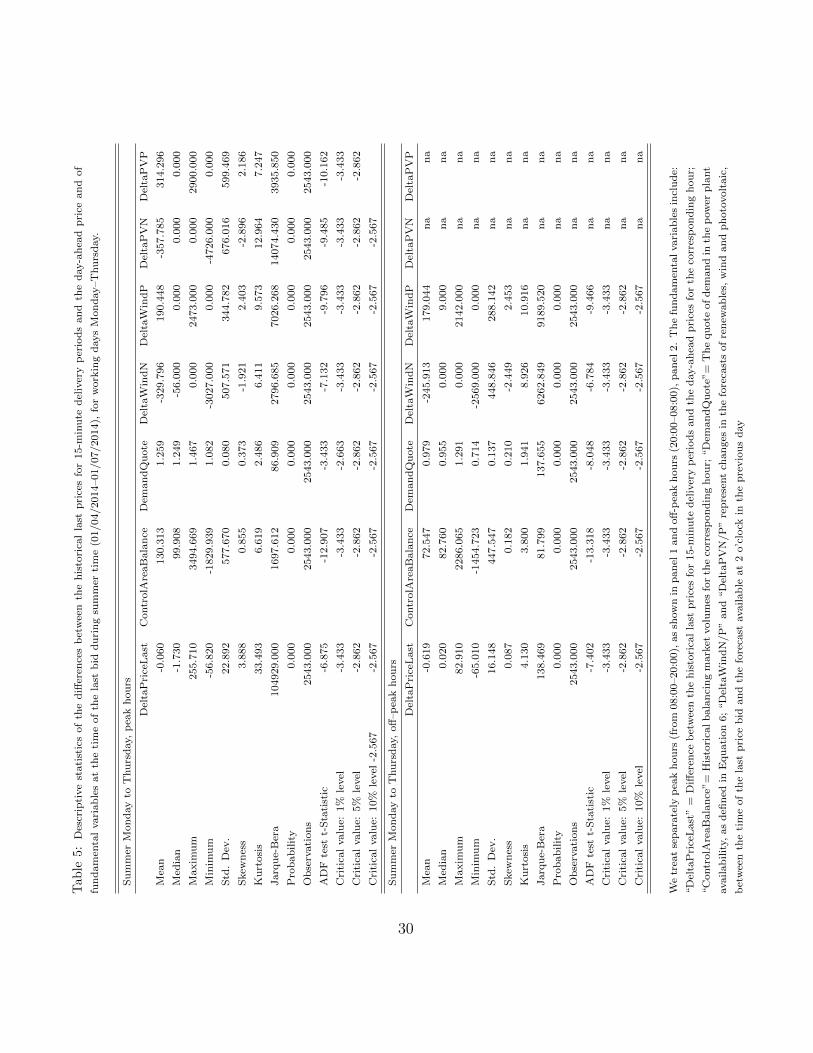
In Tables 4 and 5 we show descriptive statistics of the selected input254
variables. We distinguish between summer/winter, peak/off peak hours (as255
shown in [23]). We observe that, independent on the season, on average the256
intraday last price for 15-minute delivery periods is below the day-ahead price257
for the corresponding hour. Furthermore, the difference becomes larger and258
more volatile for off-peak than for peak hours and in winter than in summer.259
The control area balances are, on average, negative in winter and turn into260
positive in summer.261
On average, the demand quote is higher and more volatile during peak262
than in off-peak hours, which makes the planning of traditional capacity for263
the day ahead more difficult.264
To test for stationarity we perform an augmented Dickey-Fuller test (ADF265
test). For all variables we reject the null hypothesis of a unit root at a 95%266
significance level meaning that the data is stationary.267
As shown in Figures 3 and 4, there is a clear jigsaw seasonality in the268
last prices, independent on the season. Based on the information of the long-269
term dynamics of historical last prices, we control for the seasonal pattern270
by introducing dummy variables as follows:271
• Summer peak272
– We introduce one Dummy variable for each of the Q1–Q4 quarters273
for the interval 08:00–13:00 (Morning pattern)274
– We introduce one Dummy variable for each of the Q1–Q4 quarters275
for the interval 14:00–18:00 (Afternoon pattern)276
• Winter peak277
– We introduce one Dummy variable for each of the Q1–Q4 quarters278
for the interval 08:00–12:00 (Morning pattern)279
– We introduce one Dummy variable for each of the Q1–Q4 quarters280
for the interval 13:00–17:00 (Afternoon pattern)281
• Summer off-peak282
– We introduce one Dummy variable for each of the Q1–Q4 quarters283
for the interval 20:00–01:00 (Evening descending pattern)284
– We introduce one Dummy variable for each of the Q1–Q4 quarters285
for the interval 03:00–07:00 (Early morning ascending pattern)286
16

• Winter off-peak287
– We introduce one Dummy variable for each of the Q1–Q4 quarters288
for the interval 20:00–21:00 and 04:00–07:00 (Descending pattern)289
– We introduce one Dummy variable for each of the Q1–Q4 quarters290
for the interval 23:00–03:00 (Night, ascending pattern)291
The model specification reads:292
(P IDt − PDahd
t )h = ch + βhControlAreaBalancet1ht + θhDemandQuotet1
ht
+ khn(WindIDt −WindDahdt )1h
t 1nt + khp(WindIDt −
−WindDahdt )1h
t 1pt + khn(PV ID
t − PV Dahdt )1h
t 1nt
+ khp(PV IDt − PV Dahd
t )1ht 1
pt +
8∑j=1
δhjDQj
(P IDt − PDahd
t )l = cl + βlControlAreaBalancet1lt + θlDemandQuotet1
lt
+ kln(WindIDt −WindDahdt )1l
t1nt + klp(WindIDt −
−WindDahdt )1l
t1pt + kln(PV ID
t − PV Dahdt )1l
t1nt
+ klp(PV IDt − PV Dahd
t )1lt1
pt +
8∑j=1
δljDQj (7)
As threshold variable, the demand quote splits the data in two regimes:293
high/sufficient demand quote (“h”) or low (“l”). The indicator function 1p/nt294
further distinguishes in each regime between positive/negative forecasting295
errors in the renewables.296
5.2. Model for the continuous trades for quarter-hourly products297
In the second part, we examine the continuous trades for several quarter-298
hourly products. Thus, we are interested to see how delta bid prices change299
when new information on wind and PV for a certain delivery period of in-300
terest becomes available intraday. We are interested in the bidding behavior301
of market participants in the intraday electricity market as influenced by302
17

market fundamentals. In particular, we are interested to see how delta bid303
prices for a certain quarter of an hour change when new information on the304
forecasts for wind and PV becomes available. We look at the trade-off be-305
tween autoregressive terms and fundamental factors impacting the intraday306
price formation process.307
The model specification reads:308
(∆P IDt )h = ch + αh
1∆P IDt−11
ht + αh
2∆P IDt−21
ht + αh
3∆P IDt−31
ht
+ khnw (∆WindIDt )1ht 1
nt + khpw (∆WindIDt )1h
t 1pt
+ khnPV (∆PV IDt )1h
t 1nt + khpPV (∆PV ID
t )1ht 1
pt
+ γhDemandQuoteDahdt 1h
t + εhV olumeIDt 1ht + βh
√∆t
(∆P IDt )l = cl + αl
1∆P IDt−11
lt + αl
2∆P IDt−21
lt + αl
3∆P IDt−31
lt
+ klnw (∆WindIDt )1lt1
nt + klpw (∆WindIDt )1l
t1pt
+ klnPV (∆PV IDt )1l
t1nt + klpPV (∆PV ID
t )1lt1
pt
+ γlDemandQuoteDahdt 1l
t + εlV olumeIDt 1lt + βl
√∆t (8)
The examination of autocorrelation function of price changes for a cer-309
tain quarter of an hour shows that the first 3 lags of price changes should310
be selected in the autoregressive part of the model. Changes in the wind,311
∆WindIDt , and in the PV, ∆PV IDt , are real time updated forecasts, avail-312
able at the time when the bids are placed.8 V olumeIDt is the volume trade313
at the time when the price change is observed. The bids for a certain quarter314
of an hour do not occur at equal time intervals in the continuous bidding.315
In fact, market participants start bidding around 4 pm, after the day-ahead316
prices are published at EPEX and continuous trades go up to 45 minutes317
before the beginning of the delivery period. Thus, the time steps between318
consecutively placed bids are not equal, but can vary from some seconds to319
several hours. We take into account this time discontinuity by including in320
our list of explanatory variables the control variable√
∆t.321
In Tables 6 and 7 we show descriptive statistics for the price changes and322
8Results are available upon request
18

volume trades for the 15-minute continuous trading for delivery periods in323
different times of the day. We observe that the volatility of intraday price324
changes increases continuously between the morning quarter of hours (H7Q1)325
up to noon (H12Q4) and decreases again towards the evening (quarters of326
hour 18). Thus, the higher the demand, the larger the average price changes327
in the continuous trading. The volume of trades is on average the highest328
and more volatile for the first and last quarters of each one of the investigated329
hours, independent on the time of the day.330
6. Empirical results331
6.1. Modeling deviations of last prices from the day-ahead price332
The model shown in Equation (7) has been estimated for the historical333
differences between the last prices and the day-ahead prices separately for334
winter and summer and we further distinguished among peak (8 am and335
8 pm) and off-peak hours. This approach is justified by the different price336
levels in summer compared to the winter time and by the different demand337
profiles during peak and off-peak hours (see [23] for an extensive discussion338
on the seasonality of electricity prices).339
The overall OLS estimation results for each case study are shown in Ta-340
ble 8. We further tested for a threshold effect in the demand quote in each341
case. The threshold variable is the demand quote and the threshold loca-342
tion is estimated using the methodology described in section 4.2. All model343
parameters in Equations (7) are allowed to vary among regimes. We found344
evidence for significant threshold effect only in the case of winter peak case345
study. Results are available in Table 9.346
Throughout all variables are significant and show the expected sign (see347
Table 8). Dummy variables which explain the jigsaw pattern are statisti-348
cally significant and their inclusion still allows significant marginal effects of349
fundamental variables on delta prices. The coefficients of positive/negative350
forecasting errors in wind and PV are significant at 1% significance level.351
Positive forecasting errors of wind/PV signal market participants more ca-352
pacity available in the market than planned. This will have a decreasing effect353
on the residual demand and will further decrease last price bids. Viceversa,354
when updated forecasts signal less infeed from renewables than planned in355
the day ahead (negative forecasting errors), market participants will increase356
their bid prices intraday accordingly.357
19

At the time of the last price bids, market participants do not know yet the358
real control area balances, but forecasts of those are used in practice. This359
is reflected in the coefficients of balances forecasts which are statistically360
significant in all case studies and have a positive sign. Higher control area361
balances are a signal of excess demand which has not been yet balanced out in362
the intraday market, and this will be reflected in higher intraday last prices.363
We observe that the coefficient of demand quote is negative during the off-364
peak regimes, but it turns into positive during peak hours. In both summer365
and winter regimes, the mean value of demand quote in the off-peak hours is366
slightly below one, touching a maximum of 1.291 and 1.178, respectively (as367
shown in Tables 4 and 5). Thus, on average, the traditional capacity planned368
in the market covers the expected demand for the day-ahead. However,369
higher levels of demand quote (up to a maximum observed in off-peak of370
about 1.2), power producers plan less capacity for the day ahead, due to371
a higher expectation of renewables infeed in the market. It is known that372
in the night hours extreme wind infeed has been empirically observed (see373
[23]). The input from renewable energies is expected to be, on average, 20%374
of the total input production mix in Germany (see [22]). Renewables will375
be fed with priority into the grid, decreasing the residual demand. This376
will imply further that price bids in the intraday market will be in the less377
convex area of the merit order curve, thus market participants will bid lower378
prices intraday. This assumption is confirmed by the negative sign of the379
coefficients of demand quote in the off-peak hours winter/summer, as shown380
in Table 8.381
In summer peak, descriptive statistics show that on average, the demand382
quote exceeds 1.2. Thus, power producers plan less capacity in the market,383
given the volatile infeed from photovoltaic in peak hours. However, demand384
quotes above 1.2 reflect the situation where the 20% expected infeed from385
renewables will not suffice and there will be still high residual demand in the386
market. This will have an increasing effect on intraday prices in general and387
on the last prices in particular, which is confirmed by the positive sign of the388
coefficient of demand quote. This is reflected in the high maximum spreads389
between the last prices and day-ahead prices observed in summer peak, as390
shown in Table 5.391
We found no significant threshold effect in the demand quote in summer-392
related case studies and in winter off-peak. This shows that in those seasons,393
market participants adjust linearly last prices (and implicitly the spreads394
last prices-day-ahead prices) to market fundamentals. However, in winter395
20

peak time we found evidence for asymmetric behavior (see Table 9). Thus,396
a threshold in the demand quote was found significant at the level of 1.058.397
In the regime of low levels of demand quote (regime 1, < 1.058), we observe398
that coefficients are generally not statistically significant. That is, power399
producers have low expectation of renewable infeed in the day-ahead, and in400
consequence plan sufficient traditional capacity to satisfy expected demand.401
However, when demand levels are high, thus in regime 2, delta prices adjust402
linearly to forecasting errors in renewable energy, to control area balances403
and to demand quote. An increase in demand quote in this regime will404
suppress bid prices in the intraday market, since again higher demand quote405
levels reflect a high expectation of infeed from renewable energies, which406
will lower the price level. The coefficient of control area balances is positive407
and significant. This reflects two situations: if there is high infeed from408
renewables in the market, negative forecasts of control area balances will409
suppress the intraday last prices. By contrary, in the presence of high demand410
quote not fully covered by renewables infeed, positive forecasts in control area411
balances will increase intraday price bids.412
The model can be used to forecast the last prices submitted for a certain413
quarter of one hour intraday. This is based on a rigourous forecasting model414
for the control area balances. This model is highly relevant for practitioners:415
the main goal of market participants is to clear their positions in the day-416
ahead and intraday markets and avoid participating in the more expensive417
balancing market.418
6.2. Model for the continuous trades for quarter-hourly products419
We estimated the model specification shown in Equation (8) for each one420
of the following delivery periods: hour 7 (quarters 1–4), hour 12 (quarters421
1–4) and hour 18 (quarters 1–4). We aim at analysing whether the impact422
of fundamentals on the bidding behavior depends on the time of the day.423
Thus, we analyse representative delivery periods within one day: morning,424
noon peak and (for winter evening) peak. In Tables 10, 13 and 15 we show425
the overall estimation without threshold of the model shown in Equation (8)426
applied to data sorted for hours 7, 12 and 18, respectively, quarters 1–4. In427
the lower panel of the tables we show a benchmark, where we estimated the428
model without fundamental variables. We further tested for threshold effect429
in the demand quote in all case studies and found significant threshold effect430
as shown in Tables 11 and 12 for the four quarters of hour 7, and in Tables 14431
21

and 16 for each quarter of hours 12 and 18, respectively. The threshold values432
are significant, accordingly to the likelihood ratio test, as discussed in section433
4.1. The graphs and calculations corresponding to each threshold values are434
available upon request. We have tested for threshold significance also in the435
other fundamental variables, but no conclusive results were obtained.436
By comparing the values of the R2 between the lower and upper panels in437
Tables 10, 13 and 15, we observe that in the model where market fundamen-438
tals are considered, the R2s increases. The increase becomes more obvious439
for the quarters of hour 12, where market fundamentals help increasing the440
explanatory power of the model by up to 4 times.441
By examining Tables 10 and 13 we observe that during morning (quar-442
ters 1–4 hour 7) and evening (quarters 1–4 hour 18), market participants443
adjust their intraday bids to lagged price changes, which replace the role of444
fundamental variables. Thus, during morning and evening updated forecasts445
of wind and photovoltaic become less relevant. However, the coefficients of446
fundamental variables become significant during noon (see Table 13). This447
can be due to the fact that over noon there is a high demand for electricity448
in the market and in the same time it is more difficult to optimally plan449
capacity, given the highly volatile infeed from photovoltaic and wind. Thus,450
the effect of market fundamentals increases with an increased expected share451
from renewable energy. In this context, updated forecasts in wind and PV452
available at the time of the bid become highly relevant information for market453
participants who adjust their bids accordingly. Negative forecasting errors in454
wind and PV will increase intraday prices, while positive forecasting errors455
in renewables will have a suppressing effect on prices.456
In particular, by examining the threshold model applied to price changes457
for quarters 1–4 of hour 12 we can conclude an asymmetric adjustment to458
forecasting errors in renewables (see Table 14). In both quarters 1 and 2 the459
coefficients of wind forecasting errors (positive/negative) are not significant460
in regime 1 (of low demand quote), but they turn significant in regime 2.461
Similarly, in the fourth quarter of hour 12 the coefficient of negative fore-462
casting errors of wind and of positive forecasting errors of PV are significant463
only in the second regime of the demand quote. These situations justify the464
choice of demand quote as threshold variable: in the high regime of the de-465
mand quote, thus, when there is excess demand uncovered by the planned466
traditional capacity in the market, forecasting errors of renewables influence467
the bidding behavior in the intraday market. Interestingly, for quarter 3 of468
hour 12 we observe however a higher speed of adjustment of price changes to469
22

forecasting errors from renewables in the lower demand quote regime than470
in regime 2. However, this can be due to the fact that less than 10% of the471
overall observations are concentrated in regime 1.472
As already mentioned, the results of the threshold model applied to obser-473
vations in hours 7 and 18 (Tables 11 and 16) show that the role of forecasting474
errors of renewables for the morning and eyeing quarters drops. Still, pos-475
itive forecasting errors in PV will decrease prices in quarter 4 of hour 7 in476
regime 2, which reflects the ramping up effect of the sun. By contrary, during477
quarters 1–3 of hour 18, negative forecasting errors of wind will increase price478
changes intraday in the same high regime of the demand quote. In addition,479
negative forecasting errors of PV increase intraday prices in the first quarter480
of hour 18. After this quarter, however, the role of forecasting errors of PV481
drops, showing the ramping down effect of the sun.482
We observe that the coefficient of volume of trades is significant only for483
quarter 4 of hour 7 (see Table 10) and has a negative sign. This pattern484
is again observed in the threshold model for hour 7 (see Table 11). When485
we allow for threshold effect in the demand quote, the coefficient of volume486
trades for quarter 4 of hour 7 is significant and has a negative sign in regime487
1, when the demand quote is below 1.415 (see Tables 11). The observations488
in regime 1 are further split into two regimes, as shown in Table 12, where489
a second threshold has been found significant when the demand quote is at490
1.178. In the low regime, with demand quote below 1.178, we observe again491
that the coefficient of volume of trades is statistically significant and has a492
negative sign. For the last quarter of hour 7 the intraday price is below the493
average price bid for hour 7 in the day ahead due to the sun ramping up494
effect. This becomes apparent in the jigsaw pattern shown in Figures 3 and495
4. Thus, the volume of trades in quarter 4 of hour 7 corresponds to the supply496
side market participants who need to lower their conventional output, due497
to an excess of infeed from PV. This has a suppressing effect on the intraday498
prices. By contrary, the coefficient of volume trades becomes positive and499
significant in quarter 2 of hour 7 in the second sample split for this case study500
(see Table 12). Thus, when the demand quote exceeds 1.145, demand side501
volume of trades will further increase intraday prices.502
The same pattern of coefficients of volume of trades holds also for the503
results concerning quarters 1–4 for hour 12. The coefficient is significant and504
has a positive sign for the first quarter and turns into negative in quarter 4505
in the overall OLS estimation and in the upper regime of the demand quote,506
as shown in Tables 13 and 14, respectively. However, for hour 18 this effect is507
23

reverted. As shown in Tables 15 and 16, the coefficient of volume of trades is508
significant and has a negative sign for the first quarter of hour 18 and turns509
into positive in the last quarter. This reflects the sun ramping down effect,510
which causes the jigsaw pattern for the evening hours: the intraday price for511
quarter 1 is below the average price bid in the day ahead for the respective512
hours and it ends above it for quarter 4 (as shown in Figures 3 and 4). Thus,513
in quarter 1 there is an excess of capacity and supply side volume of trades514
will lower intraday prices. The opposite will happen for the last quarter of515
evening hours.516
7. Conclusion517
In this study, we investigate the bidding behavior in the intraday electric-518
ity market, in the context of a fundamental model. In particular, we shed519
light on the impact of the updates in the forecasting errors of wind and pho-520
tovoltaic (PV) on the 15-minute electricity price changes in the continuous521
bidding. We employ a unique data set of the latest forecasts of wind and PV522
available to traders prior to the placements of their price bids intraday. To523
our knowledge, this is the first study in the literature which models intra-524
day prices based on prior information on fundamentals. We further control525
for the demand/supply disequilibria, volume of trades, forecasts of control526
area balances and model the typical jigsaw seasonality pattern of 15-minute527
prices.528
Our analysis is twofold. We firstly propose a forecasting model for the529
changes between last prices bid intraday for a certain quarter of one hour530
and the corresponding day-ahead price for that hour. This is highly relevant,531
since market participants are mainly interested in squeezing their positions532
in the day-ahead or intraday markets and avoid to need the control area533
balancing market. Secondly, a fundamental model for the price changes in534
the continuous bidding is derived. We found clear evidence that the bidding535
behavior is influenced by forecasting errors in renewables, available at the536
time of the bid. In particular, intraday prices increase in negative forecasting537
errors, while positive forecasting errors have a suppressing effect on prices.538
We account for both linear and asymmetric adjustments of price changes539
of market fundamentals. The asymmetries are driven by the threshold vari-540
able demand-quote. The location of the threshold show market participants541
the proportion in which the expected demand is covered by the planned542
24

traditional capacity in the day-ahead market. Dependent whether the mar-543
ket is in the lower/upper regime of the demand-quote, market participants544
can intuitively form expectations about the expected infeed from renewable545
energies, wind and PV, in the market and adjust their bids accordingly.546
Our model desentangles the effect of market fundamentals dependent on the547
regime of the demand quote and further dependent of the time of the day.548
Tangentially, market fundamentals influence more the bidding behavior in549
the middle of the day than during mornings and evenings. There is an asym-550
metric adjustment of electricity prices with respect to both volume of trades551
and forecasting errors in renewables. Namely, in the high regime of the de-552
mand quote, where there is too little planned traditional capacity in the553
day-ahead market, market participants incorporate the information of the554
latest available forecasting errors of renewables in their bids. This effect is555
more obvious for the mid-day quarters, but less obvious during morning and556
evening hours.557
The identification of regimes in the demand quote helps also to desentan-558
gle the demand/supply side volume of trades. In the regime of high demand559
quote, demand-side volume of trades have an increasing effect on prices. Vice560
versa, supply-side volumes have a suppressing effect on intraday prices, which561
becomes obvious in the low regime of the demand quote.562
Aknowledgements563
The authors thank Hendrik Brockmeyer and Claus Liebenberger for their564
valuable input in the data collection step. We further thank Karl Frauendor-565
fer and Reik Borger for very useful discussions about the intraday markets.566
We also thank Jonas Adam for technical support with this paper.567
25

References568
[1] Karakatsani, N., Bunn, D., 2008. Intra-day and regime-switching dynamics in569
electricity price formation. Energy Economics, 30 1776–1797.570
[2] Cludius, J., Hermann, H., Matthes, F., Graichen, V., 2014. The merit order571
effect of wind and photovoltaic electricity generation in germany 20082016:572
Estimation and distributional implications. Energy Economics 44, 302313.573
[3] E., Garnier, R., Madlener, 2014. Balancing forecast errors in continuous-trade574
intraday markets. FCN WP 2/2014, RWTH Aachen University School of Busi-575
ness and Economics.576
[4] Gianfreda, A., 2010. Volatility and volume effects in european electricity spot577
markets. Econ. Notes 39 (1), 4763.578
[5] Grabber, D., 2014. Handel mit Strom aus erneuerbaren Energien. Springer579
Gabler.580
[6] Graeber, D., Kleine, A., 2013. The combination of forecasts in the trading of581
electricity from renewable energy sources. J Bus Econ 83, 409435.582
[17] Hadsell, L., Marathe, A., 2006. A tarch examination of the return volatil-583
ityvolume relationship in electricity futures. Appl. Financ. Econ. 16 (12),584
893901.585
[8] Hagemann, S., 2013. Price Determinants in the German Intraday Market for586
Electricity: An Empirical Analysis - Working Paper, Essen.587
[9] Hagemann, S., Weber, C., 2013. An Empirical Analysis of Liquidity and its588
Determinants in The German Intraday Market for Electricity - Working Pa-589
per, Essen.590
[10] Hansen, B., 1996. Inference when a nuisance parameter is not identified under591
the null hypothesis, Econometrica.592
26

[11] Hansen, B., 2000. Sample splitting and threshold estimation, Econometrica,593
68.594
[12] Hansen, B. & Seo, B., 2000. Testing for threshold cointegration in vector error595
correction models, Working Paper.596
[13] Just, S., Weber, C., 2012. Strategic behavior in the german balancing energy597
mechanism: Incentives, evidence, costs and solutions, eWL Working Paper.598
[14] Jø’nsson, T., Pinson, P., Madsen, H., 2010. On the market impact of wind599
energy forecasts. Energy Economics 32 (2), 313–320.600
[15] Ketterer, J., 2014. The impact of wind power generation on the electricity601
price in germany. Energy Economics 44, 270280.602
[16] Klaeboe, G., Eriksrud, A.L., Fleten, S.-E., 2013. Benchmarking time series603
based forecasting models for electricity balancing market prices. RPF Working604
Paper No. 2013–006.605
[17] Hadsell, L., Marathe, A., 2006. A tarch examination of the return volatil-606
ityvolume relationship in electricity futures. Appl. Financ. Econ. 16 (12),607
893901.608
[18] Mller, C., Rachev, S., Fabozzi, F., 2011. Balancing energy strategies in elec-609
tricity portfolio management. Energy Economics 22 (1), 2–11.610
[19] Nicolosi, M., Fursch, M., 2009. The impact of an increasing share of res-e on611
the conventional power market the example of germany. Z. Energiewirtschaft612
3, 246254.613
[20] Nicolosi, M., 2010. Wind power generation and power system flexibility – An614
empirical analysis of extreme events in Germany under the new negative price615
regime, Energy Policy 38 (11), 7257–7268. .616
27

[21] Paraschiv, F., 2013. Adjustment policy of deposit rates in the case of Swiss617
non-maturing savings accounts. Journal of Applied Finance & Banking, 3(2),618
271–323.619
[22] Paraschiv, F., Erni, D. & Pietsch, R., 2014. The impact of renewable energies620
on EEX day-ahead electricity prices. Energy Policy, 73, 196–210.621
[23] Paraschiv, F., Fleten, S.-E. & Schurle, M., 2015. A spot-forward model for622
electricity prices with regime shifts. Energy Economics, 47, 142–153.623
28

Tab
le4:
Des
crip
tive
stati
stic
sof
the
diff
eren
ces
bet
wee
nth
eh
isto
rica
lla
stp
rice
sfo
r15-m
inu
ted
eliv
ery
per
iod
san
dth
ed
ay-a
hea
dp
rice
an
dof
fun
dam
enta
lvari
ab
les
at
the
tim
eof
the
last
bid
du
rin
gth
ew
inte
rti
me
(01/01/2014–01/04/2014),
for
work
ing
days
Mon
day–T
hu
rsd
ay.
Win
ter
Mon
day
toT
hu
rsd
ay,
pea
kh
ou
rs
Del
taP
rice
Last
Contr
olA
reaB
ala
nce
Dem
an
dQ
uote
Del
taW
ind
ND
elta
Win
dP
Del
taP
VN
Del
taP
VP
Mea
n-0
.379
-158.2
79
1.1
55
-484.0
03
264.2
14
-301.5
59
373.0
34
Med
ian
-0.6
40
-163.6
71
1.1
65
-125.0
00
0.0
00
0.0
00
0.0
00
Maxim
um
299.2
90
3697.9
52
1.2
66
0.0
00
5180.0
00
0.0
00
4188.0
00
Min
imu
m-1
01.9
70
-3012.0
49
0.6
49
-4165.0
00
0.0
00
-7557.0
00
0.0
00
Std
.D
ev.
26.7
38
713.3
87
0.0
69
781.7
15
626.8
64
849.9
27
710.2
05
Skew
nes
s1.5
14
0.4
47
-3.3
16
-2.3
13
4.5
84
-4.6
60
2.3
80
Ku
rtosi
s15.5
35
5.9
40
20.1
10
8.3
46
29.2
78
29.9
69
8.6
95
Jarq
ue-
Ber
a16956.2
60
962.8
23
34334.3
30
5095.9
60
78971.9
70
83011.4
70
5615.8
63
Pro
bab
ilit
y0.0
00
0.0
00
0.0
00
0.0
00
0.0
00
0.0
00
0.0
00
Ob
serv
ati
on
s2447.0
00
2447.0
00
2447.0
00
2447.0
00
2447.0
00
2447.0
00
2447.0
00
AD
Fte
stt-
Sta
tist
ic-7
.653
-12.9
88
-7.2
08
-5.7
31
-6.3
18
-8.8
44
-11.9
28
CV
1%
level
-3.4
33
-3.4
33
-3.4
33
-3.4
33
-3.4
33
-3.4
33
-3.4
33
CV
5%
level
-2.8
63
-2.8
63
-2.8
63
-2.8
63
-2.8
63
-2.8
63
-2.8
63
CV
10%
level
-2.5
67
-2.5
67
-2.5
67
-2.5
67
-2.5
67
-2.5
67
-2.5
67
Win
ter
Mon
day
toT
hu
rsd
ay,
off
–p
eak
hou
rs
Del
taP
rice
Last
Contr
olA
reaB
ala
nce
Dem
an
dQ
uote
Del
taW
ind
ND
elta
Win
dP
Del
taP
VN
Del
taP
VP
Mea
n-1
.088
-150.5
79
0.9
34
-393.9
45
256.6
62
na
na
Med
ian
-0.3
00
-136.9
37
0.9
08
-88.0
00
0.0
00
na
na
Maxim
um
152.8
10
2320.6
93
1.1
78
0.0
00
4670.0
00
na
na
Min
imu
m-1
10.3
50
-2139.2
98
0.6
34
-4012.0
00
0.0
00
na
na
Std
.D
ev.
20.2
24
456.0
92
0.1
22
632.7
99
488.1
88
na
na
Skew
nes
s0.3
42
-0.0
17
0.1
78
-2.5
12
3.5
00
na
na
Ku
rtosi
s5.1
29
4.6
20
1.9
81
10.3
53
21.5
23
na
na
Jarq
ue-
Ber
a510.0
16
267.7
70
118.9
16
8087.0
61
39977.8
90
na
na
Pro
bab
ilit
y0.0
00
0.0
00
0.0
00
0.0
00
0.0
00
na
na
Ob
serv
ati
on
s2447.0
00
2447.0
00
2447.0
00
2447.0
00
2447.0
00
na
na
AD
Fte
stt-
Sta
tist
ic-7
.812
-14.5
49
-8.9
09
-6.7
64
-9.4
06
na
na
CV
1%
level
-3.4
33
-3.4
33
-3.4
33
-3.4
33
-3.4
33
na
na
CV
5%
level
-2.8
63
-2.8
63
-2.8
63
-2.8
63
-2.8
63
na
na
CV
10%
level
-2.5
67
-2.5
67
-2.5
67
-2.5
67
-2.5
67
na
na
We
trea
tse
para
tely
pea
kh
ou
rs(f
rom
08:0
0–20:0
0),
as
show
nin
pan
el1
an
doff
-pea
kh
ou
rs(2
0:0
0–08:0
0),
pan
el2.
Th
efu
nd
am
enta
lvari
ab
les
incl
ud
e:
“D
elta
Pri
ceL
ast
”=
Diff
eren
ceb
etw
een
the
his
tori
cal
last
pri
ces
for
15-m
inu
ted
eliv
ery
per
iod
san
dth
ed
ay-a
hea
dp
rice
sfo
rth
eco
rres
pon
din
gh
ou
r;
“C
ontr
olA
reaB
ala
nce
”=
His
tori
cal
bala
nci
ng
mark
etvolu
mes
for
the
corr
esp
on
din
gh
ou
r;“D
eman
dQ
uote
”=
Th
equ
ote
of
dem
an
din
the
pow
erp
lant
availab
ilit
y,as
defi
ned
inE
qu
ati
on
6;
“D
elta
Win
dN
/P
”an
d“D
elta
PV
N/P
”re
pre
sent
chan
ges
inth
efo
reca
sts
of
ren
ewab
les,
win
dan
dp
hoto
volt
aic
,
bet
wee
nth
eti
me
of
the
last
pri
ceb
idan
dth
efo
reca
stavailab
leat
2o’c
lock
inth
ep
revio
us
day
29
Tab
le5:
Des
crip
tive
stati
stic
sof
the
diff
eren
ces
bet
wee
nth
eh
isto
rica
lla
stp
rice
sfo
r15-m
inu
ted
eliv
ery
per
iod
san
dth
ed
ay-a
hea
dp
rice
an
dof
fun
dam
enta
lvari
ab
les
at
the
tim
eof
the
last
bid
du
rin
gsu
mm
erti
me
(01/04/2014–01/07/2014),
for
work
ing
days
Mon
day–T
hu
rsd
ay.
Su
mm
erM
on
day
toT
hu
rsd
ay,
pea
kh
ou
rs
Del
taP
rice
Last
Contr
olA
reaB
ala
nce
Dem
an
dQ
uote
Del
taW
ind
ND
elta
Win
dP
Del
taP
VN
Del
taP
VP
Mea
n-0
.060
130.3
13
1.2
59
-329.7
96
190.4
48
-357.7
85
314.2
96
Med
ian
-1.7
30
99.9
08
1.2
49
-56.0
00
0.0
00
0.0
00
0.0
00
Maxim
um
255.7
10
3494.6
69
1.4
67
0.0
00
2473.0
00
0.0
00
2900.0
00
Min
imu
m-5
6.8
20
-1829.9
39
1.0
82
-3027.0
00
0.0
00
-4726.0
00
0.0
00
Std
.D
ev.
22.8
92
577.6
70
0.0
80
507.5
71
344.7
82
676.0
16
599.4
69
Skew
nes
s3.8
88
0.8
55
0.3
73
-1.9
21
2.4
03
-2.8
96
2.1
86
Ku
rtosi
s33.4
93
6.6
19
2.4
86
6.4
11
9.5
73
12.9
64
7.2
47
Jarq
ue-
Ber
a104929.0
00
1697.6
12
86.9
09
2796.6
85
7026.2
68
14074.4
30
3935.8
50
Pro
bab
ilit
y0.0
00
0.0
00
0.0
00
0.0
00
0.0
00
0.0
00
0.0
00
Ob
serv
ati
on
s2543.0
00
2543.0
00
2543.0
00
2543.0
00
2543.0
00
2543.0
00
2543.0
00
AD
Fte
stt-
Sta
tist
ic-6
.875
-12.9
07
-3.4
33
-7.1
32
-9.7
96
-9.4
85
-10.1
62
Cri
tica
lvalu
e:1%
level
-3.4
33
-3.4
33
-2.6
63
-3.4
33
-3.4
33
-3.4
33
-3.4
33
Cri
tica
lvalu
e:5%
level
-2.8
62
-2.8
62
-2.8
62
-2.8
62
-2.8
62
-2.8
62
-2.8
62
Cri
tica
lvalu
e:10%
level
-2.5
67
-2.5
67
-2.5
67
-2.5
67
-2.5
67
-2.5
67
-2.5
67
Su
mm
erM
on
day
toT
hu
rsd
ay,
off
–p
eak
hou
rs
Del
taP
rice
Last
Contr
olA
reaB
ala
nce
Dem
an
dQ
uote
Del
taW
ind
ND
elta
Win
dP
Del
taP
VN
Del
taP
VP
Mea
n-0
.619
72.5
47
0.9
79
-245.9
13
179.0
44
na
na
Med
ian
0.0
20
82.7
60
0.9
55
0.0
00
9.0
00
na
na
Maxim
um
82.9
10
2286.0
65
1.2
91
0.0
00
2142.0
00
na
na
Min
imu
m-6
5.0
10
-1454.7
23
0.7
14
-2569.0
00
0.0
00
na
na
Std
.D
ev.
16.1
48
447.5
47
0.1
37
448.8
46
288.1
42
na
na
Skew
nes
s0.0
87
0.1
82
0.2
10
-2.4
49
2.4
53
na
na
Ku
rtosi
s4.1
30
3.8
00
1.9
41
8.9
26
10.9
16
na
na
Jarq
ue-
Ber
a138.4
69
81.7
99
137.6
55
6262.8
49
9189.5
20
na
na
Pro
bab
ilit
y0.0
00
0.0
00
0.0
00
0.0
00
0.0
00
na
na
Ob
serv
ati
on
s2543.0
00
2543.0
00
2543.0
00
2543.0
00
2543.0
00
na
na
AD
Fte
stt-
Sta
tist
ic-7
.402
-13.3
18
-8.0
48
-6.7
84
-9.4
66
na
na
Cri
tica
lvalu
e:1%
level
-3.4
33
-3.4
33
-3.4
33
-3.4
33
-3.4
33
na
na
Cri
tica
lvalu
e:5%
level
-2.8
62
-2.8
62
-2.8
62
-2.8
62
-2.8
62
na
na
Cri
tica
lvalu
e:10%
level
-2.5
67
-2.5
67
-2.5
67
-2.5
67
-2.5
67
na
na
We
trea
tse
para
tely
pea
kh
ou
rs(f
rom
08:0
0–20:0
0),
as
show
nin
pan
el1
an
doff
-pea
kh
ou
rs(2
0:0
0–08:0
0),
pan
el2.
Th
efu
nd
am
enta
lvari
ab
les
incl
ud
e:
“D
elta
Pri
ceL
ast
”=
Diff
eren
ceb
etw
een
the
his
tori
cal
last
pri
ces
for
15-m
inu
ted
eliv
ery
per
iod
san
dth
ed
ay-a
hea
dp
rice
sfo
rth
eco
rres
pon
din
gh
ou
r;
“C
ontr
olA
reaB
ala
nce
”=
His
tori
calb
ala
nci
ng
mark
etvolu
mes
for
the
corr
esp
on
din
gh
ou
r;“D
emand
Qu
ote
”=
Th
equ
ote
of
dem
an
din
the
pow
erp
lant
availab
ilit
y,as
defi
ned
inE
qu
ati
on
6;
“D
elta
Win
dN
/P
”an
d“D
elta
PV
N/P
”re
pre
sent
chan
ges
inth
efo
reca
sts
of
ren
ewab
les,
win
dan
dp
hoto
volt
aic
,
bet
wee
nth
eti
me
of
the
last
pri
ceb
idan
dth
efo
reca
stavailab
leat
2o’c
lock
inth
ep
revio
us
day
30

Tab
le6:
Des
crip
tive
stati
stic
sof
the
intr
ad
ay
pri
cech
an
ges
bet
wee
ntw
oco
nse
cuti
ve
bid
sfo
rth
e15-m
inu
ted
eliv
ery
per
iod
sin
the
conti
nu
ou
s
trad
ing.
We
sele
cted
4d
eliv
ery
per
iod
sd
uri
ng
morn
ing
(H7Q
1–4),
noon
pea
k(H
12Q
1–4)
an
dev
enin
gp
eak
(H18Q
1–4)
qu
art
erof
hou
rs.
H7Q
1H
7Q
2H
7Q
3H
7Q
4H
12Q
1H
12Q
2
Mea
n0.0
02
0.0
03
0.0
07
0.0
08
0.0
07
0.0
08
Med
ian
0.0
00
0.0
00
0.0
00
0.0
00
0.0
00
0.0
00
Maxim
um
62.0
00
51.0
00
74.2
90
84.9
80
80.0
00
67.6
90
Min
imu
m-7
3.9
00
-71.7
00
-101.6
80
-73.7
90
-282.0
00
-247.3
40
Std
.D
ev.
5.3
06
6.3
35
6.2
84
6.4
04
6.9
06
7.2
49
Skew
nes
s-0
.288
-0.9
40
-0.5
07
0.7
32
-14.3
28
-8.1
38
Ku
rtosi
s29.5
57
22.1
54
35.2
09
31.1
39
584.7
80
291.7
60
Jarq
ue-
Ber
a143358.3
00
75254.8
70
210973.8
00
161306.4
00
68932280.0
00
16994366.0
00
Pro
bab
ilit
y0.0
00
0.0
00
0.0
00
0.0
00
0.0
00
0.0
00
Ob
serv
ati
on
s4876.0
00
4876.0
00
4876.0
00
4876.0
00
4876.0
00
4876.0
00
AD
Fte
stt-
Sta
tist
ic-3
8.8
95
-36.2
97
-27.5
98
-37.7
81
-39.0
01
-41.7
89
Cri
tica
lvalu
e:1%
level
-3.4
31
-3.4
32
-3.4
31
-3.4
31
-3.4
31
-3.4
31
Cri
tica
lvalu
e:5%
level
-2.8
62
-2.8
62
-2.8
62
-2.8
62
-2.8
62
-2.8
62
Cri
tica
lvalu
e:10%
level
-2.5
67
-2.5
67
-2.5
67
-2.5
67
-2.5
67
-2.5
67
H12Q
3H
12Q
4H
18Q
1H
18Q
2H
18Q
3H
18Q
4
Mea
n0.0
06
0.0
02
-0.0
04
0.0
00
0.0
08
0.0
02
Med
ian
0.0
00
0.0
00
0.0
00
0.0
00
0.0
00
0.0
00
Maxim
um
89.0
00
120.0
00
110.9
90
55.9
00
84.0
00
112.1
20
Min
imu
m-1
80.0
00
-92.0
00
-91.9
00
-68.0
00
-85.9
90
-112.1
20
Std
.D
ev.
8.0
11
6.5
76
6.1
67
5.9
88
6.3
50
6.9
39
Skew
nes
s-3
.725
0.7
54
2.2
75
-0.3
58
-0.0
87
-1.5
51
Ku
rtosi
s121.8
92
55.3
60
68.0
92
24.4
33
28.7
64
58.0
12
Jarq
ue-
Ber
a2883104.0
00
557458.1
00
865012.6
00
93434.7
50
134859.8
00
616793.7
00
Pro
bab
ilit
y0.0
00
0.0
00
0.0
00
0.0
00
0.0
00
0.0
00
Ob
serv
ati
on
s4876.0
00
4876.0
00
4876.0
00
4876.0
00
4876.0
00
4876.0
00
AD
Fte
stt-
Sta
tist
ic-5
3.7
56
-72.0
44
-46.7
98
-33.8
27
-49.2
34
-26.3
63
Cri
tica
lvalu
e:1%
level
-3.4
31
-3.4
31
-3.4
31
-3.4
31
-3.4
31
-3.4
31
Cri
tica
lvalu
e:5%
level
-2.8
62
-2.8
62
-2.8
62
-2.8
62
-2.8
62
-2.8
62
Cri
tica
lvalu
e:10%
level
-2.5
67
-2.5
67
-2.5
67
-2.5
67
-2.5
67
-2.5
67
31

Tab
le7:
Des
crip
tive
stati
stic
sof
the
volu
me
trad
esb
etw
een
two
con
secu
tive
bid
sfo
rth
e15-m
inu
ted
eliv
ery
per
iod
sin
the
conti
nu
ou
str
ad
ing.
We
sele
cted
4d
eliv
ery
per
iod
sd
uri
ng
morn
ing
(H7Q
1–4),
noon
pea
k(H
12Q
1–4)
an
dev
enin
gp
eak
(H18Q
1–4)
qu
art
erof
hou
rs.
H7Q
1H
7Q
2H
7Q
3H
7Q
4H
12Q
1H
12Q
2
Mea
n15.0
48
8.2
13
8.3
94
14.0
29
10.0
04
6.9
76
Med
ian
12.0
00
5.0
00
5.2
00
10.2
00
5.0
00
2.5
00
Maxim
um
150.0
00
60.6
00
70.0
00
100.0
00
234.9
00
75.0
00
Min
imu
m0.1
00
0.1
00
0.1
00
0.1
00
0.1
00
0.1
00
Std
.D
ev.
12.8
97
8.8
76
8.8
56
12.5
25
11.7
70
9.7
35
Skew
nes
s1.4
55
1.8
23
1.8
20
1.4
14
2.9
79
2.1
77
Ku
rtosi
s7.6
96
7.1
59
7.4
85
6.0
62
33.3
88
8.5
74
Jarq
ue-
Ber
a6201.3
08
6215.6
72
6778.6
03
3528.3
71
194828.9
00
10163.7
40
Pro
bab
ilit
y0.0
00
0.0
00
0.0
00
0.0
00
0.0
00
0.0
00
Ob
serv
ati
on
s4876.0
00
4876.0
00
4876.0
00
4876.0
00
4876.0
00
4876.0
00
AD
Fte
stt-
Sta
tist
ic-3
3.1
83
-30.1
76
-24.8
59
-34.6
69
-37.0
50
-28.1
99
Cri
tica
lvalu
e:1%
level
-3.4
31
-3.4
32
-3.4
31
-3.4
31
-3.4
31
-3.4
31
Cri
tica
lvalu
e:5%
level
-2.8
62
-2.8
62
-2.8
62
-2.8
62
-2.8
62
-2.8
62
Cri
tica
lvalu
e:10%
level
-2.5
67
-2.5
67
-2.5
67
-2.5
67
-2.5
67
-2.5
67
H12Q
3H
12Q
4H
18Q
1H
18Q
2H
18Q
3H
18Q
4
Mea
n8.9
75
11.6
06
13.6
90
8.4
80
8.1
36
12.6
88
Med
ian
4.2
00
6.3
00
10.0
00
4.1
00
4.0
00
9.0
00
Maxim
um
100.0
00
100.0
00
179.0
00
95.5
00
195.6
00
200.0
00
Min
imu
m0.1
00
0.1
00
0.1
00
0.1
00
0.1
00
0.1
00
Std
.D
ev.
11.1
45
12.9
17
13.5
46
10.3
68
10.3
28
13.0
99
Skew
nes
s1.8
45
1.6
61
1.7
88
1.9
60
3.2
00
2.8
42
Ku
rtosi
s7.0
07
6.7
17
10.4
50
7.5
33
30.8
15
26.2
07
Jarq
ue-
Ber
a6026.3
35
5050.2
12
13874.8
80
7295.6
22
165508.5
00
115984.0
00
Pro
bab
ilit
y0.0
00
0.0
00
0.0
00
0.0
00
0.0
00
0.0
00
Ob
serv
ati
on
s4876.0
00
4876.0
00
4876.0
00
4876.0
00
4876.0
00
4876.0
00
AD
Fte
stt-
Sta
tist
ic-2
6.1
56
-25.0
07
-34.2
58
-33.7
75
-31.5
87
-37.0
25
Cri
tica
lvalu
e:1%
level
-3.4
31
-3.4
31
-3.4
31
-3.4
31
-3.4
31
-3.4
31
Cri
tica
lvalu
e:5%
level
-2.8
62
-2.8
62
-2.8
62
-2.8
62
-2.8
62
-2.8
62
Cri
tica
lvalu
e:10%
level
-2.5
67
-2.5
67
-2.5
67
-2.5
67
-2.5
67
-2.5
67
32

Table 8: Estimation results of the model shown in Equation 7. Global OLS without
thresholdDependent variable Delta Last Price- Price DayAhedd
Summer off-peak Summer peak Winter off-peak Winter peak
Coeff Std. err. Coeff Std. err. Coeff Std. err. Coeff Std. err.
Co 7.388* (1.971) -20.956* (6.128) 14.469* (4.762) -9.015 (10.354)
DemandQ -7.438* (2.159) 10.929** (4.852) -12.715* (4.605) -0.354 (8.728)
Balancing 0.007* (0.001) 0.008* (0.001) 0.014* (0.001) 0.009* (0.001)
DeltaWindP -0.005* (0.001) -0.002** (0.001) -0.003* (0.001) -0.003* (0.001)
DeltaWindN -0.007* (0.001) -0.012* (0.001) -0.004* (0.001) -0.004* (0.001)
DeltaPVP – – -0.003* (0.001) – – -0.003* (0.001)
DeltaPVN – – -0.004* (0.001) – – -0.005* (0.001)
DQ1M 10.170* (1.112) 10.022* (1.462) -4.561* (1.729) 23.808* (2.340)
DQ2M 3.515* (1.144) 2.192 (1.507) -5.094* (1.717) 11.336* (2.148)
DQ3M -6.519* (1.122) -1.486 (1.463) -3.148 (1.704) 2.740 (2.207)
DQ4M -10.454* (1.139) -6.031* (1.622) -1.187 (1.719) -0.548 (2.296)
DQ1A -13.845* (1.219) -8.111* (1.539) 3.114 (1.848) -6.098* (2.173)
DQ2A -6.852* (1.229) 0.268 (1.374) -0.948 (1.802) 3.203 (2.016)
DQ3A 0.349 (1.161) 3.458** (1.341) -4.578** (1.793) 16.773* (2.118)
DQ4A 4.842* (1.203) 13.132* (1.451) -4.568** (1.825) 25.588* (2.294)
Rsquared 35.43% 37.99% 28.76% 36.63%
No. Obs. 2543 2483 2447 2363
Standard errors are shown in parenthesis. * and **, denote a test statistic is statistically significant at
the 1% and 5% level of significance, respectively.
33

Table 9: Winter peak, threshold estimation results. Threshold variable: Demand Quote
Threshold estimation (threshold variable DemandQ)
Dependent variable Delta Last Price- Price Dahd
Regime 1 Regime 2
Threshold value <= 1.058 > 1.058
Coeff Std. Err. Coeff Std. Err.
Co -48.973* (15.527) 63.563* (22.987)
DemandQ 26.810** (12.806) -61.545* (19.412)
Balancing 0.003 (0.002) 0.010* (0.001)
DeltaWindP -0.004 (0.003) -0.002** (0.001)
DeltaWindN -0.006** (0.003) -0.004* (0.001)
DeltaPVP -0.003 (0.002) -0.004* (0.001)
DeltaPVN -0.006* (0.001) -0.006* (0.001)
DQ1M 41.322* (8.710) 21.500* (2.324)
DQ2M 21.880* (7.985) 10.443* (2.129)
DQ3M 4.806 (7.948) 3.682 (2.205)
DQ4M 2.266 (8.284) 0.298 (2.329)
DQ1A -8.175 (7.420) -1.367 (2.340)
DQ2A 8.898 (7.325) 3.440 (2.207)
DQ3A 30.651* (7.536) 12.192* (2.235)
DQ4A 45.249* (7.616) 17.453* (2.369)
Rsquared 48.61% 35.93%
No. Obs. 652 1711
Standard errors are shown in parenthesis. *, and ** denote a test statistic is statistically significant at
the 1% and 5% level of significance, respectively.
34

Table 10: Estimation results hour 7, Quarters 1–4, global OLS without threshold, entire
sample
OLS estimation of the model including fundamental variables
Dependent variable Delta Price
H7Q1 H7Q2 H7Q3 H7Q4
Coeff Std. err. Coeff Std. err. Coeff Std. err. Coeff Std. err.
Co 0.288 (0.645) -0.450 (0.965) -1.392 (1.139) -1.102 (0.858)
DeltaPrice1 -0.208* (0.030) -0.320* (0.032) -0.244* (0.035) -0.281* (0.033)
DeltaPrice2 -0.157* (0.032) -0.159* (0.021) -0.121* (0.027) -0.175* (0.020)
DeltaPrice3 -0.084* (0.017) -0.080* (0.018) -0.084* (0.019) -0.086* (0.016)
DemandQuote -0.300 (0.543) 0.381 (0.829) 0.966 (0.965) 1.011 (0.736)
Volume 0.008 (0.005) 0.015 (0.009) 0.001 (0.009) -0.020* (0.006)
SqrTimeStep -0.833 (1.420) -1.212 (1.359) 4.101* (1.319) 4.127* (1.547)
DeltaWindIntrP 0.0001 (0.0002) 0.0002 (0.0002) -0.001 (0.001) -0.001 (0.001)
DeltaWindIntrN-0.001* (0.0001) 0.0001 (0.0002) 0.0002 (0.001) 0.001 (0.001)
DeltaPVIntraP 0.0001 (0.001) 0.001 (0.001) 0.0002 (0.001) 0.002 (0.002)
DeltaPVIntraN 0.001 (0.001) 0.002** (0.001) -0.001 (0.001) 0.000 (0.001)
Rsquared 5.989% 10.930% 7.333% 9.481%
No. Obs. 6979 4873 4977 7175
OLS estimation of the autoregressive model, excluding fundamental variables
Dependent variable Delta Price
H7Q1 H7Q2 H7Q3 H7Q4
Coeff Std. err. Coeff Std. err. Coeff Std. err. Coeff Std. err.
Co 0.004 (0.061) 0.005 (0.086) 0.010 (0.086) 0.007 (0.072)
DeltaPrice1 -0.207* (0.012) -0.321* (0.014) -0.243* (0.014) -0.276* (0.012)
DeltaPrice2 -0.158* (0.012) -0.159* (0.015) -0.119* (0.014) -0.175* (0.012)
DeltaPrice3 -0.083* (0.012) -0.080* (0.014) -0.085* (0.014) -0.082* (0.012)
Rsquared 5.055% 9.718% 6.170% 8.085%
No. Obs. 6979 4873 4977 7175
Standard errors are shown in parenthesis. *, and ** denote a test statistic is statistically significant at the
1% and 5% level of significance, respectively. The interpretation of variables is: DeltaPrice(x)=lagged price
changes 1–3; DemandQuote=demand quote; Volume=volume of trades; SqrTimeStep=√
∆t; DeltaWind-
IntrP/N=positive/negative forecasting errors in wind; DeltaPVIntraP/N=positive/negative forecasting
errors in PV.
35

Tab
le11
:E
stim
atio
nre
sult
sh
ou
r7,
Qu
art
ers
1–4,
Fir
stS
am
ple
Sp
lit
Dep
end
ent
vari
ab
leD
elta
Pri
ce
H7Q
1H
7Q
2H
7Q
3H
7Q
4
Regim
e1
Th
resh
old
valu
e<
=1.1
61∗
<=
0.7
57∗
<=
0.8
28∗
<=
1.4
15∗
Coeff
Std
.er
r.C
oeff
Std
.er
r.C
oeff
Std
.er
r.C
oeff
Std
.er
r.
Co
0.7
65
(1.3
65)
16.4
16*
(7.6
88)
-16.6
89
(13.2
79)
-1.5
61**
(0.8
22)
Del
taP
rice
1-0
.184*
(0.0
36)
-0.1
55**
(0.0
73)
-0.2
21*
(0.0
83)
-0.2
55*
(0.0
30)
Del
taP
rice
2-0
.193*
(0.0
38)
-0.1
87*
(0.0
44)
-0.0
87
(0.0
85)
-0.1
69*
(0.0
20)
Del
taP
rice
3-0
.098*
(0.0
22)
-0.0
05
(0.0
51)
-0.0
75
(0.0
57)
-0.0
86*
(0.0
17)
Dem
an
dQ
uote
-0.8
44
(1.2
53)
-21.9
80**
(10.7
06)
19.2
29
(17.2
52)
1.4
16**
(0.7
00)
Volu
me
0.0
10
(0.0
07)
0.0
44
(0.1
08)
-0.0
61
(0.0
53)
-0.0
18*
(0.0
06)
SqrT
imeS
tep
0.0
54
(1.9
59)
1.3
70
(9.5
74)
44.8
73*
(12.3
33)
3.8
20**
(1.5
71)
Del
taW
ind
Intr
P0.0
00
(0.0
00)
-0.0
56*
(0.0
18)
-0.1
34*
(0.0
25)
-0.0
01
(0.0
01)
Del
taW
ind
Intr
N0.0
00
(0.0
01)
-0.0
13
(0.0
17)
0.0
14**
(0.0
07)
0.0
01
(0.0
01)
Del
taP
VIn
traP
0.0
01
(0.0
02)
0.0
01
(0.0
13)
0.0
07
(0.0
24)
0.0
03*
(0.0
01)
Del
taP
VIn
traN
0.0
00
(0.0
01)
0.0
12
(0.0
11)
0.0
11
(0.0
08)
0.0
00
(0.0
01)
Rsq
uared
6.0
81%
67.4
60%
63.4
97%
9.0
53%
No.
Ob
s.4090
82
111
6984
H7Q
1H
7Q
2H
7Q
3H
7Q
4
Regim
e2
Th
resh
old
valu
e>
1.1
61∗
>0.7
57∗
>0.8
28∗
>1.4
15∗
Coeff
Std
.er
r.C
oeff
Std
.er
r.C
oeff
Std
.er
r.C
oeff
Std
.er
r.
Co
0.3
88
(1.3
05)
-0.3
68
(1.0
62)
-0.1
72
(1.0
95)
-58.0
38
(120.1
83)
Del
taP
rice
1-0
.233*
(0.0
50)
-0.3
18*
(0.0
31)
-0.2
36*
(0.0
35)
-0.3
63*
(0.1
35)
Del
taP
rice
2-0
.081
(0.0
49)
-0.1
56*
(0.0
22)
-0.1
09*
(0.0
20)
-0.2
31*
(0.0
88)
Del
taP
rice
3-0
.047
(0.0
25)
-0.0
84*
(0.0
19)
-0.0
81*
(0.0
18)
-0.0
93**
(0.0
47)
Dem
an
dQ
uote
-0.2
10
(1.0
23)
0.3
02
(0.9
04)
-0.0
96
(0.9
14)
39.7
13
(83.7
69)
Volu
me
0.0
04
(0.0
06)
0.0
14
(0.0
09)
0.0
02
(0.0
09)
-0.0
35
(0.0
39)
SqrT
imeS
tep
-3.0
34
(1.9
30)
-0.9
05
(1.3
72)
4.5
28*
(1.2
91)
43.4
01*
(17.2
20)
Del
taW
ind
Intr
P-0
.002**
(0.0
01)
0.0
00
(0.0
00)
-0.0
01
(0.0
01)
-0.0
52
(0.0
36)
Del
taW
ind
Intr
N-0
.001
(0.0
01)
0.0
00
(0.0
00)
0.0
00
(0.0
01)
-0.0
06
(0.0
36)
Del
taP
VIn
traP
0.0
01
(0.0
02)
0.0
01
(0.0
01)
0.0
00
(0.0
01)
-0.0
29*
(0.0
04)
Del
taP
VIn
traN
0.0
01
(0.0
01)
0.0
02**
(0.0
01)
-0.0
01
(0.0
01)
-0.0
27
(0.0
55)
Rsq
uared
10.0
94%
10.6
59%
7.3
49%
47.6
04%
No.
Ob
s.2889
4791
4850
191
Sta
nd
ard
erro
rsare
show
nin
pare
nth
esis
.*,
an
d**
den
ote
ate
stst
ati
stic
isst
ati
stic
ally
sign
ifica
nt
at
the
1%
an
d5%
level
of
sign
ifica
nce
,
resp
ecti
vel
y.T
he
inte
rpre
tati
on
of
vari
ab
les
is:
Del
taP
rice
(x)=
lagged
pri
cech
an
ges
1–3;
Dem
an
dQ
uote
=d
eman
dqu
ote
;V
olu
me=
volu
me
of
trad
es;
SqrT
imeS
tep
=√
∆t;
Del
taW
ind
Intr
P/N
=p
osi
tive/
neg
ati
ve
fore
cast
ing
erro
rsin
win
d;
Del
taP
VIn
traP
/N
=p
osi
tive/
neg
ati
ve
fore
cast
ing
erro
rsin
PV
.
36

Table 12: Estimation results hour 7, Quarters 2,4, Second Sample Split. For Quarter 2 the
second regime identified in the first sample split (Table 11) has been further checked for
threshold effect. For Quarter 4 the observations in regime 1 (Table 11) have been further
checked for threshold effect.Dependent variable Delta Price
Regime 1
H7Q2 H7Q4
Threshold value <= 1.145∗ <= 1.178∗Coeff Std. err. Coeff Std. err.
Co -4.367 (3.103) -2.411 (1.412)
DeltaPrice1 -0.431* (0.041) -0.287* (0.036)
DeltaPrice2 -0.242* (0.032) -0.180* (0.023)
DeltaPrice3 -0.132* (0.029) -0.082* (0.019)
DemandQuote 4.051 (2.847) 2.224 (1.284)
Volume -0.014 (0.013) -0.019* (0.007)
SqrTimeStep 1.178 (1.807) 4.501* (1.694)
DeltaWindIntrP -0.001* (0.000) -0.001 (0.001)
DeltaWindIntrN -0.001 (0.001) 0.000 (0.001)
DeltaPVIntraP 0.000 (0.002) -0.001 (0.001)
DeltaPVIntraN 0.001 (0.001) 0.002 (0.002)
Rsquared 18.171% 9.526%
No. Obs. 2175 4605
Regime 2
H7Q2 H7Q4
Threshold value > 1.145∗ > 1.178∗Coeff Std. err. Coeff Std. err.
Co -0.826 (2.130) 3.845 (4.117)
DeltaPrice1 -0.227* (0.045) -0.168* (0.042)
DeltaPrice2 -0.102* (0.029) -0.091* (0.028)
DeltaPrice3 -0.058** (0.023) -0.090 (0.047)
DemandQuote 0.536 (1.724) -3.034 (3.344)
Volume 0.043* (0.012) -0.013 (0.011)
SqrTimeStep -2.138 (1.950) 1.134 (3.719)
DeltaWindIntrP 0.000 (0.001) -0.002** (0.001)
DeltaWindIntrN 0.000 (0.001) 0.001 (0.003)
DeltaPVIntraP 0.001 (0.001) 0.006 (0.004)
DeltaPVIntraN 0.003* (0.001) -0.005* (0.001)
Rsquared 7.361% 19.427%
No. Obs. 2576 1665
Standard errors are shown in parenthesis. *, and ** denote a test statistic is statistically significant at the
1% and 5% level of significance, respectively. The interpretation of variables is: DeltaPrice(x)=lagged price
changes 1–3; DemandQuote=demand quote; Volume=volume of trades; SqrTimeStep=√
∆t; DeltaWind-
IntrP/N=positive/negative forecasting errors in wind; DeltaPVIntraP/N=positive/negative forecasting
errors in PV.37

Table 13: Estimation results hour 12, Quarters 1–4, global OLS without threshold
OLS estimation of the model including fundamental variables
Dependent variable Delta Price
H12Q1 H12Q2 H12Q3 H12Q4
Coeff Std. err. Coeff Std. err. Coeff Std. err. Coeff Std. err.
Co -0.558 (0.672) -0.674 (0.977) -0.111 (0.765) -0.032 (0.799)
DeltaPrice1 -0.175** (0.086) -0.167* (0.043) -0.207* (0.038) -0.140* (0.020)
DeltaPrice2 -0.071** (0.032) -0.040 (0.023) -0.077** (0.036) -0.079* (0.020)
DeltaPrice3 -0.102 (0.060) -0.018 (0.017) -0.039 (0.021) -0.020 (0.013)
DemandQuote 0.109 (0.499) 0.408 (0.755) 0.156 (0.578) 0.088 (0.635)
Volume 0.053* (0.019) 0.012 (0.009) -0.012 (0.009) -0.013** (0.006)
SqrTimeStep 0.423 (1.570) 1.868 (1.365) 1.010 (1.348) 1.683 (1.853)
DeltaWindIntrP -0.001* (0.000) -0.001 (0.001) -0.001* (0.000) -0.001* (0.000)
DeltaWindIntrN -0.001* (0.000) -0.001 (0.001) -0.001 (0.001) -0.002** (0.001)
DeltaPVIntraP -0.002** (0.001) -0.002** (0.001) -0.002** (0.001) -0.004* (0.001)
DeltaPVIntraN 0.000 (0.001) -0.001 (0.001) -0.002** (0.001) -0.002** (0.001)
Rsquared 7.296% 4.705% 7.011% 8.411%
No. Obs. 6859 5449 6558 7931
OLS estimation of the autoregressive model excluding fundamental variables
Dependent variable Delta Price
H12Q1 H12Q2 H12Q3 H12Q4
Coeff Std. err. Coeff Std. err. Coeff Std. err. Coeff Std. err.
Co 0.006 (0.077) 0.004 (0.099) 0.005 (0.092) 0.003 (0.066)
DeltaPrice1 -0.172* (0.012) -0.167* (0.014) -0.206* (0.012) -0.137* (0.011)
DeltaPrice2 -0.065* (0.012) -0.041* (0.014) -0.077* (0.013) -0.078* (0.011)
DeltaPrice3 -0.099* (0.012) -0.018 (0.014) -0.041* (0.012) -0.019 (0.011)
Rsquared 3.715% 2.733% 4.219% 2.187%
No. Obs. 6859 5449 6558 7931
Standard errors are shown in parenthesis. *, and ** denote a test statistic is statistically significant at the
1% and 5% level of significance, respectively. The interpretation of variables is: DeltaPrice(x)=lagged price
changes 1–3; DemandQuote=demand quote; Volume=volume of trades; SqrTimeStep=√
∆t; DeltaWind-
IntrP/N=positive/negative forecasting errors in wind; DeltaPVIntraP/N=positive/negative forecasting
errors in PV.
38

Table 14: Estimation results hour 12, Quarters 1–4, First Sample Split
Dependent variable Delta Price
Regime 1
H12Q1 H12Q2 H12Q3 H12Q4
Threshold value <= 1.245∗ <= 1.245∗ <= 1.146∗ <= 1.197∗Coeff Std. err. Coeff Std. err. Coeff Std. err. Coeff Std. err.
Co -0.669 (1.982) -0.693 (3.302) 0.421 (2.418) 0.365 (3.418)
DeltaPrice1 -0.202 (0.118) -0.126* (0.043) -0.191** (0.075) -0.108* (0.031)
DeltaPrice2 -0.065 (0.043) -0.042** (0.021) -0.142 (0.085) -0.082** (0.040)
DeltaPrice3 -0.099 (0.078) -0.010 (0.018) -0.023 (0.078) -0.030 (0.017)
DemandQuote 0.163 (1.685) 0.518 (2.798) 0.036 (2.104) -0.378 (3.069)
Volume 0.070** (0.028) 0.022 (0.012) -0.007 (0.029) 0.003 (0.016)
SqrTimeStep -1.363 (2.119) -0.205 (1.886) -9.905 (5.560) 0.880 (2.436)
DeltaWindIntrP 0.000 (0.001) 0.000 (0.001) 0.005* (0.002) -0.001 (0.001)
DeltaWindIntrN -0.001 (0.001) -0.001 (0.001) -0.006* (0.001) 0.002 (0.002)
DeltaPVIntraP -0.003* (0.001) -0.003* (0.001) -0.007** (0.003) -0.002 (0.002)
DeltaPVIntraN 0.001 (0.001) -0.001 (0.001) -0.002 (0.002) -0.003* (0.001)
Rsquared 9.155% 3.806% 27.371% 7.764%
No. Obs. 3911 3052 487 2438
Regime 2
H12Q1 H12Q2 H12Q3 H12Q4
Threshold value > 1.245∗ > 0.757∗ > 1.146∗ > 1.197∗Coeff Std. err. Coeff Std. err. Coeff Std. err. Coeff Std. err.
Co 0.125 (1.349) -1.036 (1.809) -0.037 (0.928) 0.405 (0.944)
DeltaPrice1 -0.094** (0.040) -0.256* (0.060) -0.208* (0.040) -0.155* (0.022)
DeltaPrice2 -0.108 (0.040) -0.046 (0.053) -0.072 (0.038) -0.075 (0.020)
DeltaPrice3 -0.099** (0.043) -0.035 (0.035) -0.039 (0.022) -0.011 (0.018)
DemandQuote -0.216 (0.965) 0.630 (1.304) 0.065 (0.693) -0.163 (0.692)
Volume 0.018** (0.008) -0.006 (0.013) -0.012 (0.010) -0.021* (0.006)
SqrTimeStep 1.140 (1.439) 3.942** (1.758) 2.263 (1.191) -0.097 (1.700)
DeltaWindIntrP -0.002* (0.000) -0.002** (0.001) -0.001* (0.000) -0.001 (0.001)
DeltaWindIntrN -0.001* (0.000) -0.002** (0.001) -0.001 (0.001) -0.002** (0.001)
DeltaPVIntraP 0.000 (0.001) -0.001 (0.001) -0.002** (0.001) -0.002** (0.001)
DeltaPVIntraN -0.001 (0.001) -0.002** (0.001) -0.001 (0.001) -0.004* (0.001)
Rsquared 8.868% 10.760% 6.590% 11.624%
No. Obs. 2948 2397 6071 5493
Standard errors are shown in parenthesis. *, and ** denote a test statistic is statistically significant at the
1% and 5% level of significance, respectively. The interpretation of variables is: DeltaPrice(x)=lagged price
changes 1–3; DemandQuote=demand quote; Volume=volume of trades; SqrTimeStep=√
∆t; DeltaWind-
IntrP/N=positive/negative forecasting errors in wind; DeltaPVIntraP/N=positive/negative forecasting
errors in PV.
39
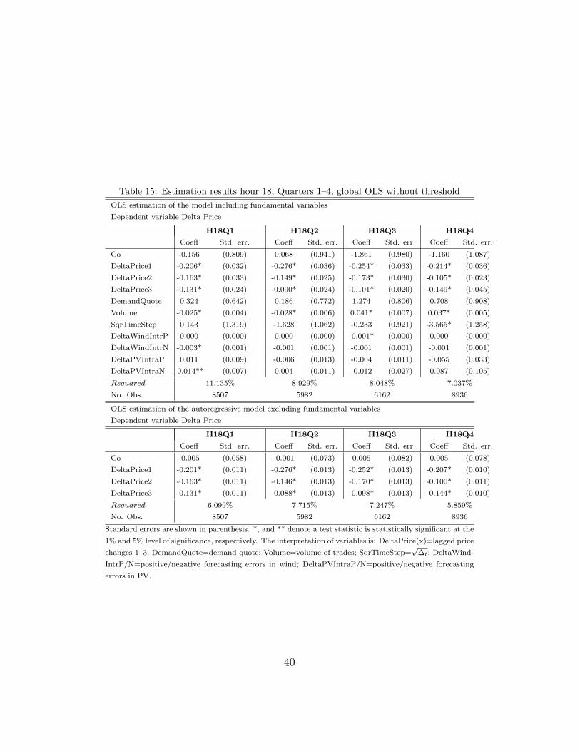
Table 15: Estimation results hour 18, Quarters 1–4, global OLS without threshold
OLS estimation of the model including fundamental variables
Dependent variable Delta Price
H18Q1 H18Q2 H18Q3 H18Q4
Coeff Std. err. Coeff Std. err. Coeff Std. err. Coeff Std. err.
Co -0.156 (0.809) 0.068 (0.941) -1.861 (0.980) -1.160 (1.087)
DeltaPrice1 -0.206* (0.032) -0.276* (0.036) -0.254* (0.033) -0.214* (0.036)
DeltaPrice2 -0.163* (0.033) -0.149* (0.025) -0.173* (0.030) -0.105* (0.023)
DeltaPrice3 -0.131* (0.024) -0.090* (0.024) -0.101* (0.020) -0.149* (0.045)
DemandQuote 0.324 (0.642) 0.186 (0.772) 1.274 (0.806) 0.708 (0.908)
Volume -0.025* (0.004) -0.028* (0.006) 0.041* (0.007) 0.037* (0.005)
SqrTimeStep 0.143 (1.319) -1.628 (1.062) -0.233 (0.921) -3.565* (1.258)
DeltaWindIntrP 0.000 (0.000) 0.000 (0.000) -0.001* (0.000) 0.000 (0.000)
DeltaWindIntrN -0.003* (0.001) -0.001 (0.001) -0.001 (0.001) -0.001 (0.001)
DeltaPVIntraP 0.011 (0.009) -0.006 (0.013) -0.004 (0.011) -0.055 (0.033)
DeltaPVIntraN -0.014** (0.007) 0.004 (0.011) -0.012 (0.027) 0.087 (0.105)
Rsquared 11.135% 8.929% 8.048% 7.037%
No. Obs. 8507 5982 6162 8936
OLS estimation of the autoregressive model excluding fundamental variables
Dependent variable Delta Price
H18Q1 H18Q2 H18Q3 H18Q4
Coeff Std. err. Coeff Std. err. Coeff Std. err. Coeff Std. err.
Co -0.005 (0.058) -0.001 (0.073) 0.005 (0.082) 0.005 (0.078)
DeltaPrice1 -0.201* (0.011) -0.276* (0.013) -0.252* (0.013) -0.207* (0.010)
DeltaPrice2 -0.163* (0.011) -0.146* (0.013) -0.170* (0.013) -0.100* (0.011)
DeltaPrice3 -0.131* (0.011) -0.088* (0.013) -0.098* (0.013) -0.144* (0.010)
Rsquared 6.099% 7.715% 7.247% 5.859%
No. Obs. 8507 5982 6162 8936
Standard errors are shown in parenthesis. *, and ** denote a test statistic is statistically significant at the
1% and 5% level of significance, respectively. The interpretation of variables is: DeltaPrice(x)=lagged price
changes 1–3; DemandQuote=demand quote; Volume=volume of trades; SqrTimeStep=√
∆t; DeltaWind-
IntrP/N=positive/negative forecasting errors in wind; DeltaPVIntraP/N=positive/negative forecasting
errors in PV.
40
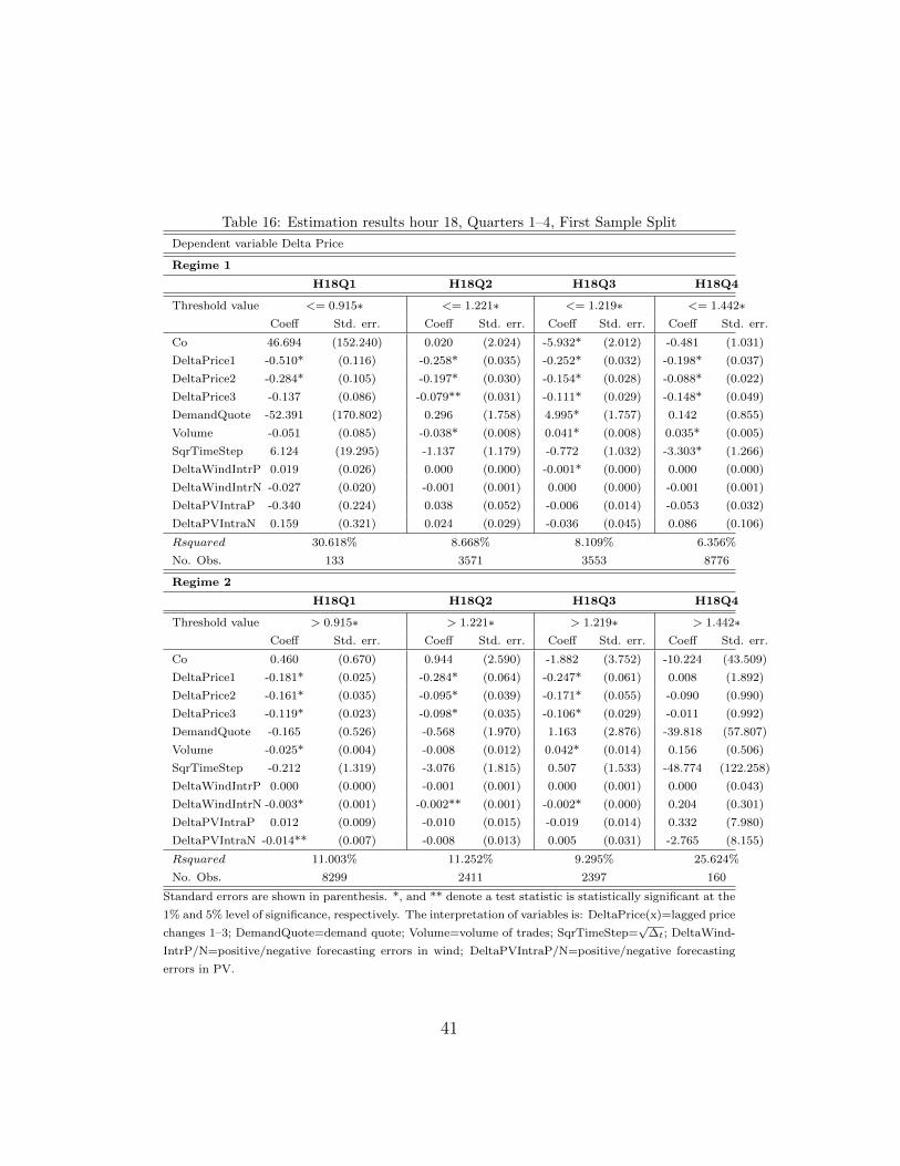
Table 16: Estimation results hour 18, Quarters 1–4, First Sample Split
Dependent variable Delta Price
Regime 1
H18Q1 H18Q2 H18Q3 H18Q4
Threshold value <= 0.915∗ <= 1.221∗ <= 1.219∗ <= 1.442∗Coeff Std. err. Coeff Std. err. Coeff Std. err. Coeff Std. err.
Co 46.694 (152.240) 0.020 (2.024) -5.932* (2.012) -0.481 (1.031)
DeltaPrice1 -0.510* (0.116) -0.258* (0.035) -0.252* (0.032) -0.198* (0.037)
DeltaPrice2 -0.284* (0.105) -0.197* (0.030) -0.154* (0.028) -0.088* (0.022)
DeltaPrice3 -0.137 (0.086) -0.079** (0.031) -0.111* (0.029) -0.148* (0.049)
DemandQuote -52.391 (170.802) 0.296 (1.758) 4.995* (1.757) 0.142 (0.855)
Volume -0.051 (0.085) -0.038* (0.008) 0.041* (0.008) 0.035* (0.005)
SqrTimeStep 6.124 (19.295) -1.137 (1.179) -0.772 (1.032) -3.303* (1.266)
DeltaWindIntrP 0.019 (0.026) 0.000 (0.000) -0.001* (0.000) 0.000 (0.000)
DeltaWindIntrN -0.027 (0.020) -0.001 (0.001) 0.000 (0.000) -0.001 (0.001)
DeltaPVIntraP -0.340 (0.224) 0.038 (0.052) -0.006 (0.014) -0.053 (0.032)
DeltaPVIntraN 0.159 (0.321) 0.024 (0.029) -0.036 (0.045) 0.086 (0.106)
Rsquared 30.618% 8.668% 8.109% 6.356%
No. Obs. 133 3571 3553 8776
Regime 2
H18Q1 H18Q2 H18Q3 H18Q4
Threshold value > 0.915∗ > 1.221∗ > 1.219∗ > 1.442∗Coeff Std. err. Coeff Std. err. Coeff Std. err. Coeff Std. err.
Co 0.460 (0.670) 0.944 (2.590) -1.882 (3.752) -10.224 (43.509)
DeltaPrice1 -0.181* (0.025) -0.284* (0.064) -0.247* (0.061) 0.008 (1.892)
DeltaPrice2 -0.161* (0.035) -0.095* (0.039) -0.171* (0.055) -0.090 (0.990)
DeltaPrice3 -0.119* (0.023) -0.098* (0.035) -0.106* (0.029) -0.011 (0.992)
DemandQuote -0.165 (0.526) -0.568 (1.970) 1.163 (2.876) -39.818 (57.807)
Volume -0.025* (0.004) -0.008 (0.012) 0.042* (0.014) 0.156 (0.506)
SqrTimeStep -0.212 (1.319) -3.076 (1.815) 0.507 (1.533) -48.774 (122.258)
DeltaWindIntrP 0.000 (0.000) -0.001 (0.001) 0.000 (0.001) 0.000 (0.043)
DeltaWindIntrN -0.003* (0.001) -0.002** (0.001) -0.002* (0.000) 0.204 (0.301)
DeltaPVIntraP 0.012 (0.009) -0.010 (0.015) -0.019 (0.014) 0.332 (7.980)
DeltaPVIntraN -0.014** (0.007) -0.008 (0.013) 0.005 (0.031) -2.765 (8.155)
Rsquared 11.003% 11.252% 9.295% 25.624%
No. Obs. 8299 2411 2397 160
Standard errors are shown in parenthesis. *, and ** denote a test statistic is statistically significant at the
1% and 5% level of significance, respectively. The interpretation of variables is: DeltaPrice(x)=lagged price
changes 1–3; DemandQuote=demand quote; Volume=volume of trades; SqrTimeStep=√
∆t; DeltaWind-
IntrP/N=positive/negative forecasting errors in wind; DeltaPVIntraP/N=positive/negative forecasting
errors in PV.
41