Embed Size (px)
Citation preview

Theory, Policy, Institutions: Papers from the Carnegie-Rochester Conference Series on Public Policy Karl Brunner and Alan Meltzer (eds.) ©Elsevier Science Publishers B.V. (North-Holland), 1983
ECONOMETRIC POLICY EVALUATION: A CRITIQUE
Robert E. Lucas, Jr.
1. Introduction
257
The fact that nominal prices and wages tend to rise more rapidly at the peak
of the business cycle than they do in the trough has been well recognized from the
time when the cycle was first perceived as a distinct phenomenon. The inference
that permanent inflation will therefore induce a permanent economic high is no
doubt equally ancient, yet it is only recently that this notion has undergone the
mysterious transformation from obvious fallacy to cornerstone of the theory of
economic policy. This transformation did not arise from new developments in economic theo-
ry. On the contrary, as soon as Phelps and others made the first serious attempts
to rationalize the apparent trade-off in modern theoretical terms, the zero-degree
homogeneity of demand and supply functions was re-discovered in this new con
text (as Friedman predicted it would be) and re-named the "natural rate hypothe
sis"} It arose, instead, from the younger tradition of the econometric forecasting
models, and from the commitment on the part of a large fraction of economists
to the use of these models for quantitative policy evaluation. These models have
implied the existence of long-run unemployment-inflation trade-offs ever since
the "wage-price sectors" were first incorporated and they promise to do so in the
future although the "terms" of the trade-off continue to shift.2 This clear-cut conflict between two rightly respected traditions - theoreti
cal and econometric - caught those of us who viewed the two as harmoniously
complementary quite by surprise. At first, it seemed that the conflict might be
resolved by somewhat fancier econometric footwork. On the theoretical level,
one hears talk of a "disequilibrium dynamics" which will somehow make money
illusion respectable while going beyond the sterility of ~ = k(p_pe). Without un
derestimating the ingenuity of either econometricians or theorists, it seems to me
appropriate to entertain the possibility that reconciliation along both of these
lines will fail, and that one of these traditions is fundamentally in error.
The thesis of this essay is that it is the econometric tradition, or more pre-
1See Phelps et aI. [311,Phelps'earlier [301 and Friedman (13). 2The earliest-;';;e-price sector embodying the "trade-off' is (as far as I know) in the 1955 version of the Klein.Goldberger model (19). It has persisted, with minimal conceptual change, into all current generation forecasting models. The subsequent shift of the "trade-off' relationship to center stage in policy discussions appears due primarily to Phillips (32) and Samuelson and Solow [331.
Reprinted from The Phillips Curve and Labor Markets, Carnegie-Rochester Conference Series on Public Policy, Volume 1 (1976), pp. 19-46.
258 R.E. Lucas. Jr.
cisely, the "theory .of economic policy" based on this tradition, which is in need
of major revision. More particularly, I shall argue that the features which lead to
success in short-term forecasting are unrelated to quantitative policy evaluation,
that the major econometric models are (well) designed to perform the former
task only, and that simulations using these models can, in principle, provide.!!Q
useful information as to the actual consequences of alternative economic policies.
These contentions will be based not on deviations between estimated and "true" structure prior to a policy change but on the deviations between the prior "true"
structure and the "true" structure prevailing afterwards.
Before turning to details, I should like to advance two disclaimers. First,as is
true with any technically difficult and novel area of science, econometric model
building is subject to a great deal of ill-informed and casual criticism. Thus mod
els are condemned as being "too big" (with equal insight, I suppose one could
fault smaller models for being "too little"), too messy, too simplistic (that is, not
messy enough), and, the ultimate blow, inferior to "naive" models. Surely the in
creasing sophistication of the "naive" alternatives to the major forecasting models
is the highest of tributes to the remarkable success of the latter. I hope I can suc
ceed in disassociating the criticism which follows from any denial of the very im
portant advances in forecasting ability recorded by the econometric models, and
of the promise they offer for advancement of comparable importance in the fu
ture.
One may well define a critique as a paper which does not fully engage the
vanity of its author. In this spirit, let me offer a second disclaimer. There is little
in this essay which is not implicit (and perhaps to more discerning readers, expli
cit) in Friedman [11], Muth [29] and, still earlier, in Knight [21]. For that mat
ter, the criticisms I shall raise against currently popular applications of econome
tric theory have, for the most part, been anticipated by the major original contri
butors to that theory.3 Nevertheless, the case for sustained inflation, based en
tirely on econometric simulations, is attended now with a seriousness it has not
commanded for many decades_ It may, therefore, be worthwhile to attempt to
trace this case back to its foundation, and then to examine again the scientific ba
sis of this foundation itself.
2. The Theory of Economic Policy
Virtually all quantitative macro-economic policy discussions today are con
ducted within a theoretical framework which I shall call "the theory of economic
3See in particular Marschak's discussion in [lSi (helpfuUy recaUed to me by T. D. WaUace) and Tinbergen's in [361. especiaUy his discussion of "qualitative policy" in ch. 5, pp. 149-185.
Econometric policy evaluation 259
policy",(following Tinbergen [35]). The essentials of this framework are so wide
ly known and subscribed to that it may be superfluous to devote space to their re
view. On the other hand, since the main theme of this paper is the inadequacy of
this framework, it is probably best to have an explicit version before us.
One describes the economy in a time period t by a vector y t of state varia
bles, a vector xt of exogeneous forcing variables, and a vector ft of independent
(through time), identically distributed random shocks. The motion of the econo
my is determined by a difference equation
the distribution of ft, and a description of the temporal behavior of the forcing
variables, x t. The function f is taken to be fIXed but not directly known; the
task of empiricists is then to estimate f. For practical purposes, one usually
thinks of estimating the values of a fixed parameter vector e, with
f(y,x,f) == F(y,x,e,f)
and F being specified in advance.
Mathematically, the sequence {Xt} of forcing vectors is regarded as being
"arbitrary" (that is, it is not characterized stochastically). Since the past Xt val
ues are observed, this causes no difficulty in estimating e, and in fact simplifies
the theoretical estimation problem slightly. For forecasting, one is obliged to in
sert forecasted Xt values into F. With knowledge of the function F and e, policy evaluation is a straight
forward matter. A policy is viewed as a specification of present and future values
of some components of {Xt}. With the other components somehow specified,
the stochastic behavior of {y t,Xt,f t } from the present on is specified, and func
tionaIs defined on this sequence are well-defined random variables, whose mo
ments may be calculated theoretically or obtained by numerical simulation.
Sometimes, for example, one wishes to examine the mean value of a hypothetical
"social objective function", such as
~ i3tu(y t,Xt,ft) t = 0
under alternative policies. More usually, one is interested in the "operating char
acteristics" of the system under alternative policies. Thus, in this standard con
text, a "long-run Phillips curve" is simply a plot of average inflation - unemploy-
260 R.E. Lucas, Jr.
ment pairs under a range of hypothetical policies.4
Since one cannot treat e as known in practice, the actual problem
of policy evaluation is somewhat more complicated. The fact that e is esti
mated from past sample values affects the above moment calculations for small
samples; it also makes policies which promise to sharpen estimates of e relatively
more attractive. These considerations complicate without, I think, essentially al
tering the theory of economic policy as sketched above. Two features of this theoretical framework deserve special comment. The
first is the uneasy relationship between this theory of economic policy and tradi
tional economic theory. The components of the vector-valued function Fare
behavioral relationships - demand functions; the role of theory may thus be
viewed as suggesting forms for F, or in Samuelson's terms, distributing zeros
throughout the Jacobian of F. This role for theory is decidedly secondary: mi
croeconomics shows surprising power to rationalize individual econometric rela
tionships in a variety of ways. More significantly, this micro-economic role for
theory abdicates the task of describing the aggregate behavior of the system en
tirely to the econometrician. Theorists suggest forms for consumption, invest
ment, price and wage setting functions separately; these suggestions, if useful, influence individual components of F. The aggregate behavior of the system then
is whatever it is.S Surely this point of view (though I doubt if many would now
endorse it in so bald a form) accounts for the demise of traditional "business cy
cle theory" and the widespread acceptance of a Phillips "trade-off' in the absence
of'!!!!y aggregative theoretical model embodying such a relationship.
Secondly, one must emphasize the intimate link between short-term fore
casting and long-term simulations within this standard framework. The variance
of short-term forecasts tends to zero with the variance of et; as the latter becomes
small, so also does the variance of estimated behavior of {y t } conditional on hy
pothetical policies { X t }. Thus forecasting accuracy in the short-run implies relia
bility of long-term policy evaluation.
3. Adaptive Forecasting
There are many signs that practicing econometricians pay little more than
lip-service to the theory outlined in the preceding section. The most striking is
the indifference of econometric forecasters to data series prior to 1947. Within
the theory of economic policy, more observations always sharpen parameter esti-
4See, for example, de Menil and Enzler (6), Hirsch (16) and Hymans (17).
SThe ill·fated Brookings model project was probably the Ultimate expression of this view.
Econometric policy evaluation 261
mates and forecasts, and observations on "extreme" Xt values particularly so;
yet even the readily available annual series from 1929-1946 are rarely used as a
check on the post-war fits. A second sign is the frequent and frequently important refitting of econome
tric relationships. The revisions of the wage-price sector now in progress are a
good example.6 The continuously improving precision of the estimates of e within the fixed structure F, predicted by the theory, does not seem to be occur
ring in practice. Finally, and most suggestively, is the practice of using patterns in recent re
siduals to revise intercept estimates for forecasting purposes. For example, if a
"run" of positive residuals (predicted less actual) arises in an equation in recent
periods, one revises the estimated intercept downward by their average amount.
This practice accounts, for example, for the superiority of the actual Wharton
forecasts as compared to forecasts based on the published version of the model. 7
It should be emphasized that recounting these discrepancies between theory
and practice is not to be taken as criticism of econometric forecasters. Certainly
if new observations are better accounted for by new or modified equations, it
would be foolish to continue to forecast using the old relationships. The point is
simply that, econometrics textbooks not withstanding, current forecasting prac
tice is not conducted within the framework of the theory of economic policy, and
the unquestioned success of the forecasters should not be construed as evidence
for the soundness or reliability of the structure proposed in that theory.
An alternative structure to that underlying the theory of economic policy
has recently been proposed (in [3] and [5]) by Cooley and Prescott. The struc
ture is of interest in the present context, since optimal forecasting within it shares
many features with current forecasting practice as just described. Instead of
treating the parameter vector e as fixed, Cooley and Prescott view it as a random
variable following the random walk
where h)t} is a sequence of independent, identically distributed random variables.
Maximum likelihood forecasting under this alternative framework ("adap
tive regression") resembles "exponential smoothing" on the observations, with
observations in the distant past receiving a small "weight" - very much as in
6See, for example, Gonion [14).
7 A good account of this and other aspects of foreca<ting in theOlY and practice is provided by Klein (20). A fuUer treatment is available in Evans and Klein [9).

262 R.E. Lucas, Jr.
usual econometric practice; similarly, recent forecast errors are used to adjust the
estimates. Using both artificial data and economic time series, Cooley and Pres
cott have shown (in [4)) that adaptive methods have good short-term forecasting
properties when compared to even relatively sophisticated versions of the "fixed
e" regression model. As Klein and others have remarked, this advantage is shared
by actual large-model forecasts (that is, model forecasts modified by the forecast
er's jUdgment) over mechanical forecasts using the published versions of the model.8
Cooley and Prescott have proposed adaptive regression as a normative fore
casting method. I am using it here in a positive sense: as an idealized "model" of
the behavior of large-model forecasters. If the model is, as I believe, roughly ac
curate, it serves to reconcile the assertion that long-term policy evaluations based
on econometric models are meaningless with the acknowledgment that the fore
cast accuracy of these models is good and likely to become even better. Under the
adaptive structure, a small standard error of short-term forecasts is consistent
with infinite variance of the long-term operating characteristics of the system.
4. Theoretical Considerations: General
To this point, I have argued simply that the standard, stable-parameter view
of econometric theory and quantitative policy evaluation appears not to match
several important characteristics of econometric practice, while an alternative
general structure, embodying stochastic parameter drift, matches these character
istics very closely. This argument is, if accepted, sufficient to establish that the
"long-run" implications of current forecasting models are without content, and
that the short-term forecasting ability of these models provides no evidence of the
accuracy to be expected from simulations of hypothetical policy rules.
These points are, I think, important, but their implications for the future are
unclear. After all, the major econometric models are still in their first, highly suc
cessful, decade. No one, surely, expected the initial parameterizations of these
models to stand forever, even under the most optimistic view of the stability of
the unknown, underlying structure. Perhaps the adaptive character of this early
stage' of macro-economic forecasting is merely the initial groping for the true
structure which, however ignored in statistical theory, all practitioners knew to
be necessary. If so, the arguments of this paper are transitory debating points, ob
solete soon after they are written down. Personally, I would not be sorry if this
were the case, but I do not believe it is. I shall try to explain why, beginning with
ieneralities, and then, in the following section, introducing examples. See Klein [201.
Econometric policy evaluation 263
In section 2, we discussed an economy characterized by
The function F and parameter vector e are derived from decision rules (demand
and supply functions) of agents in the economy, and these decisions are, theoreti
cally, optimal given the situation in which each agent is placed. There is, as re
marked above, no presumption that (F,e) will be easy to discover, but it ~ the
central assumption of the theory of economic policy that once they..!!!!.. (approxi
mately) known, they will remain stable under arbitrary changes in the behavior
of the forcing sequence { x t }.
For example, suppose a reliable model (F,e) is in hand, and one wishes to
use it to assess the consequences of alternative monetary and fiscal policy rules
(choices of xO,xl ,x2'"'' where t = 0 is "now"). According to the theory of eco
nomic policy, one then simulates the system under alternative policies (theoretical
ly or numerically) and compares outcomes by some criterion. For such compari
sons to have any meaning, it is essential that the structure (F,e) not vary systema
tically with the choice of {Xt }.
Everything we know about dynamic economic theory indicates that this
presumption is unjustified. First, the individual decision problem: "find an opti
mal decision rule when certain parameters (future prices, say) follow 'arbitrary'
paths" is simply not well formulated. Only trivial problems in which agents can
safely ignore the future can be formulated under such a vague description of mar
ket constraints. Even to obtain the decision rules underlying (F,e) then, we have
to attribute to individuals some view of the behavior of the future values of varia
bles of concern to them. This view, in conjunction with other factors, determines
their optimum decision rules. To assume stability of (F,e) under alternative poli
cy rules is thus to assume that agents' views about the behavior of shocks to the.
system are invariant under changes in the true behavior of these shocks. Without
this extreme assumption, the kinds of policy simulations called for by the theory
of economic policy are meaningless.
It is likely that the "drift" in e which the adaptive models describe stoch
astically reflects, in part, the adaptation of the decision rules of agents to the
changing character of the series they are trying to forecast. 9 Since this adapta
tion will be in most (though not all) cases slow, one is not surprised that adaptive
9This is not to suggest th at all parameter dri ft is due to this source. For example, shifts in production func· tions due to technological change are probably well described by a random walk scheme.
264 R.E. Lucas, Jr.
methods can improve the short-term forecasting abilities of the econometric mo
dels. For longer term forecasting and policy simulations, however, ignoring the
systematic sources of drift will lead to large, unpredictable errors.
5. Theoretical Considerations: Examples
If these general theoretical observations on the likelihood of systematic
"parametric drift" in the face of variations in the structure of shocks are correct,
it should be possible to confirm them by examination of the specific decision
problems underlying the major components of aggregative models. I shall discuss
in turn consumption, investment, and the wage-price sector, or Phillips curve. In
each case, the "right hand variables" will, for simplicity, be taken as "exogenous"
(as components of {Xt }). The thought-experiments matching this assumption,
and the adaptations necessary for simultaneous equations, are too well known to
require comment.
5.1 Consumption
The easiest example to discuss with confidence is the aggregate consumption
function since, due to Friedman [II], Muth [28] and Modigliani, Brumberg and
Ando [2], [27], it has both a sound theoretical rationale and an unusually high
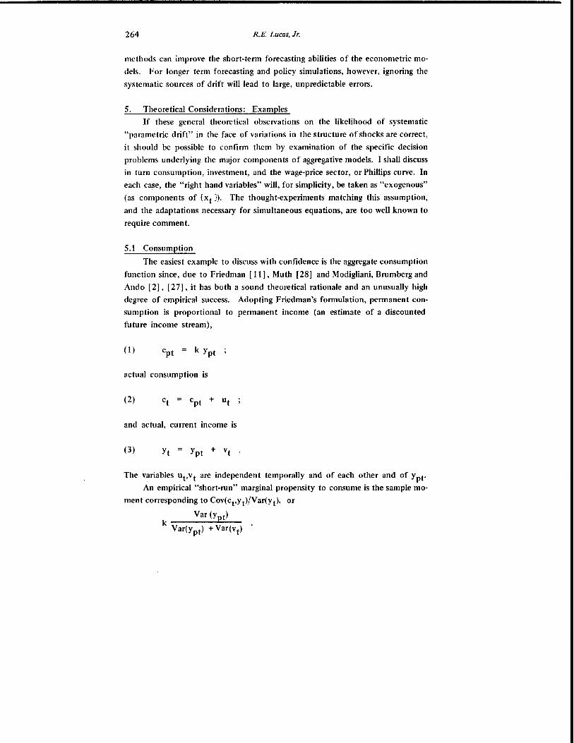
degree of empirical success. Adopting Friedman's formulation, permanent con
sumption is proportional to permanent income (an estimate of a discounted
future income stream),
(1 ) Cpt = k Y pt
actual consumption is
and actual, current income is
(3) Yt = ypt + Vt .
The variables Ut,Vt are independent temporally and of each other and of ypt.
An empirical "short-run" marginal propensity to consume is the sample mo
ment corresponding to Cov(Ctst)/Var(Yt), or
Var (ypt) k ----"--'---
Var(ypt) + Var(vt )
Econometric policy evaluation 265
Now as long as these moments are viewed as subjective parameters in the heads of
consumers, this model lacks content. Friedman, however, viewed them as true
moments, known to consumers, the logical step which led to the cross-sectional
tests which provided the most striking confirmation of his permanent income hy
pothesis. IO
This central equating of a true probability distribution and the subjective
distribution on which decisions are based was termed rational expectations by
Muth, who developed its implications more generally (in [29). In particular, in
[28], Muth found the stochastic behavior of income over time under which
Friedman's identification of permanent income as an expommtially weighted sum
of current and lagged observations on actual income was consistent with optimal
forecasting on the part of agents. 1 1
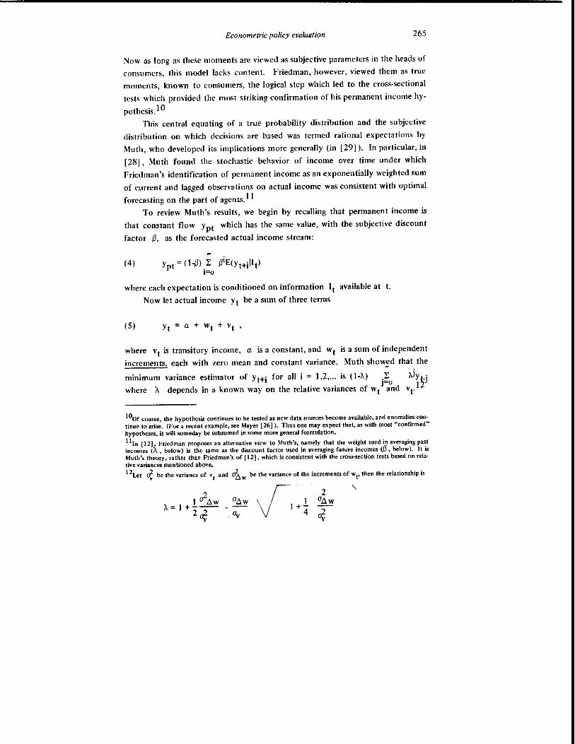
To review Muth's results, we begin by recalling that permanent income is
that constant flow ypt which has the same value, with the subjective discount
factor {3, as the forecasted actual income stream:
where each expectation is conditioned on information It available at t.
Now let actual income Yt be a sum of three terms
(5) Yt = a + Wt + Vt '
where Vt is transitory income, a is a constant, and Wt is a sum of independent
increments, each with zero mean and constant variance. Muth show;d that the
minimum variance estimator of Yt+i for all i = 1,2, ... is (l-X) .~o xjYt_j
where X depends in a known way on the relative variances of w/ and Vt· 12
100f course, the hypothesis continues to be tested as new data sources become available, and anomalies continue to arise. (For a recent example, see Mayer [26]). Thus one may expect that, as with most "confirmed" hypotheses, it will someday be subsumed in some more general formulation.
111n [12], Friedman proposes an alternative view to Muth's, namely that the weight used in averaging past incomes (X , below) is the same as the discount factor used in averaging future incomes <i3, below). It is Muth's theory, rather than Friedman's of [12], which is consistent with the cross-section tests based on relative variances mentioned above.
12Let ~ be the variance of vt
and ciw be the variance of the increments of wt' then the relationship is
266 RE. Lucas, Jr.
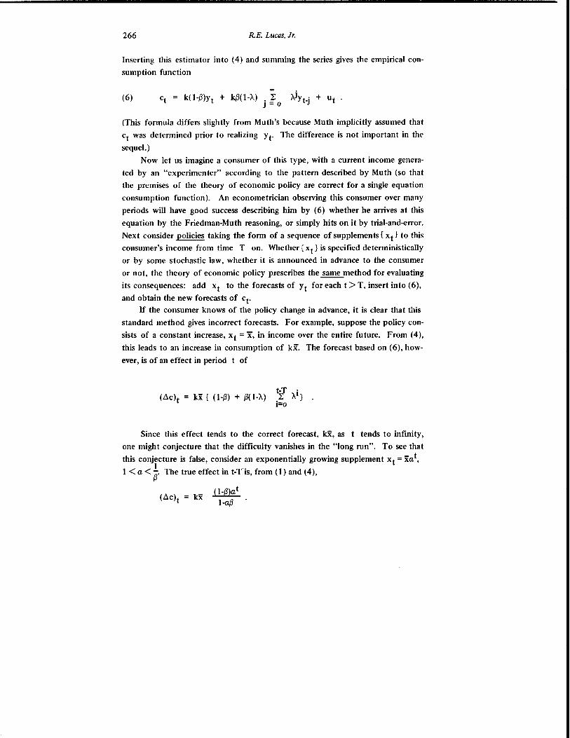
Inserting this estimator into (4) and summing the series gives the empirical con
sumption function
(This formula differs slightly from Muth's because Muth implicitly assumed that
Ct was determined prior to realizing y t. The difference is not important in the
sequeL)
Now let us imagine a consumer of this type, with a current income genera
ted by an "experimenter" according to the pattern described by Muth (so that
the premises of the theory of economic policy are correct for a single equation
consumption function). An econometrician observing this consumer over many
periods will have good success describing him by (6) whether he arrives at this
equation by the Friedman-Muth reasoning, or simply hits on it by trial-and-error.
N-ext consider policies taking the form of a sequence of supplements { Xt} to this
consumer's income from time T on. Whether {Xt} is specified deterministically
or by some stochastic law, whether it is announced in advance to the consumer
or not, the theory of economic policy prescribes the ~method for evaluating
its consequences: add Xt to the forecasts of Yt for each t> T, insert into (6),
and obtain the new forecasts of Ct. If the consumer knows of the policy change in advance, it is clear that this
standard method gives incorrect forecasts. For example, suppose the policy con
sists of a constant increase, Xt = X, in income over the entire future. From (4),
this leads to an increase in c011Sumption of kx. The forecast based on (6), how
ever, is of an effect in period t of
kx { (1-13) + 13(1-X)
Since this effect tends to the correct forecast, kx, as t tends to infinity,
one might conjecture that the difficulty vanishes in the "long run". To see that
this conjecture is faIse, consider an exponentially growing supplement Xt = xa t, t < a <~. The true effect in t-Tis, from (t ) and (4),
~ (~c)t = kx t-a13
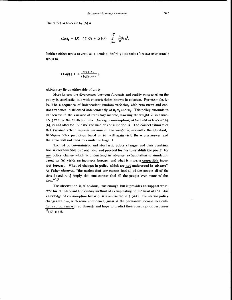
Econometric policy evaluation
The effect as forecast by (6) is
{ (l-{3) + (3(l-A) t-T L
j=o
267
Neither effect tends to zero, as t tends to infinity; the ratio (forecast over actual)
tends to
a@(l-A) (l-a{3){ I + (l-{3)( a-A)
which may lie on either side of unity.
More interesting divergences between forecasts and reality emerge when the
policy is stochastic, but with characteristics known in advance. For example, let
{Xt } be a sequence of independent random variables, with zero mean and con
stant variance, distributed independently of Ut,Vt and Wt. This policy amounts to
an increase in the variance of transitory income, lowering the weight A in a man
ner given by the Muth formula. Average consumption, in fact and as forecast by
(6), is not affected, but the variance of consumption is. The correct estimate of
this variance effect requires revision of the weight A; evidently the standard,
fixed-parameter prediction based on (6) will again yield the wrong answer, and
the error will not tend to vanish for large t.
The list of deterministic and stochastic policy changes, and their combina
tion is inexhaustible but one need not proceed further to establish the point: for
!!!!y.. policy change which is understood in advance, extrapolation or simulation
based on (6) yields an incorrect forecast, and what is more, a correctibly incor
rect forecast. What of changes in policy which are not understood in advance?
As Fisher observes, "the notion that one cannot fool all of the people all of the
time [need not] imply that one cannot fool all the people even some of the time.,,13
The observation is, if obvious, true enough; but it provides no support what
ever for the standard forecasting method of extrapolating on the basis of (6). Our
knowledge of consumption behavior is summarized in (l )-(4). For certain policy
changes we can, with some confidence, guess at the pennanent income recalcula
tions consumers will go through and hope to predict their consumption responses
13[ 101, p. 113.

268 R.E. Lucas, Jr.
with some accuracy. For other types of policies, particularly those involving de
liberate "fooling" of consumers, it will not be at all clear how to apply (I H 4),
and hence impossible to forecast. Obviously, in such cases, there is no reason to
imagine that forecasting with (6) will be accurate either.
S.2 Taxation and Investment Demand In [IS], Hall and Jorgenson provided quantitative estimates of the conse
quences, current and lagged, of various tax policies on the demand for producers'
durable equipment. Their work is an example of the current state of the art of
conditional forecasting at its best. The general method is to use econometric esti
mates of a Jorgensonian investment function, which captures all of the relevant
tax structure in a single implicit rental price variable, to simulate the effects of al
ternative tax policies. An implicit assumption in this work is that any tax change is regarded as
a permanent, once-and-for-all change. Insofar as this assumption is false over the
sample period, the econometric estimates are subject to bias. 14 More important
for this discussion, the conditional forecasts will be valid Q!!!y for tax changes be
lieved to be permanent by taxpaying corporations. For many issues in public finance, this obvious qualification would properly
be regarded as a mere technicality. For Keynesian counter-cyclical policy, how
ever, it is the very heart of the issue. The whole point, after all, of the investment
tax credit is that it be viewed a'i temporary, so that it can serve as an inducement
to firms to reschedule their investment projects. It should be clear that the fore
casting methods used by Hall and Jorgenson (and, of course, by other econome
tricians) cannot be expected to yield even order-of-magnitude estimates of the ef
fects of explicitly temporary tax adjustments. To pursue this issue further, it will be useful to begin with an explicit ver
sion of the standard accelerator model ofinvestment behavior. We imagine a con
stant returns industry in which each firm has a constant output-capital ratio A.
Using a common notation for variables at both the firm and industry level, let kt
denote capital at the beginning of year t. Output during t is Akt· Investment
during the year, it, affects next period's capital according to
141n particular, the low estimates' of 'a' (see [ 15], Table 2, p. 400), which should equal capital's share in val· ue added, are probably due to a sizeable transitoty component in avariable which is treated theoretically as though it were subject to permanent chllllges only.
Econometric policy evaluation 269
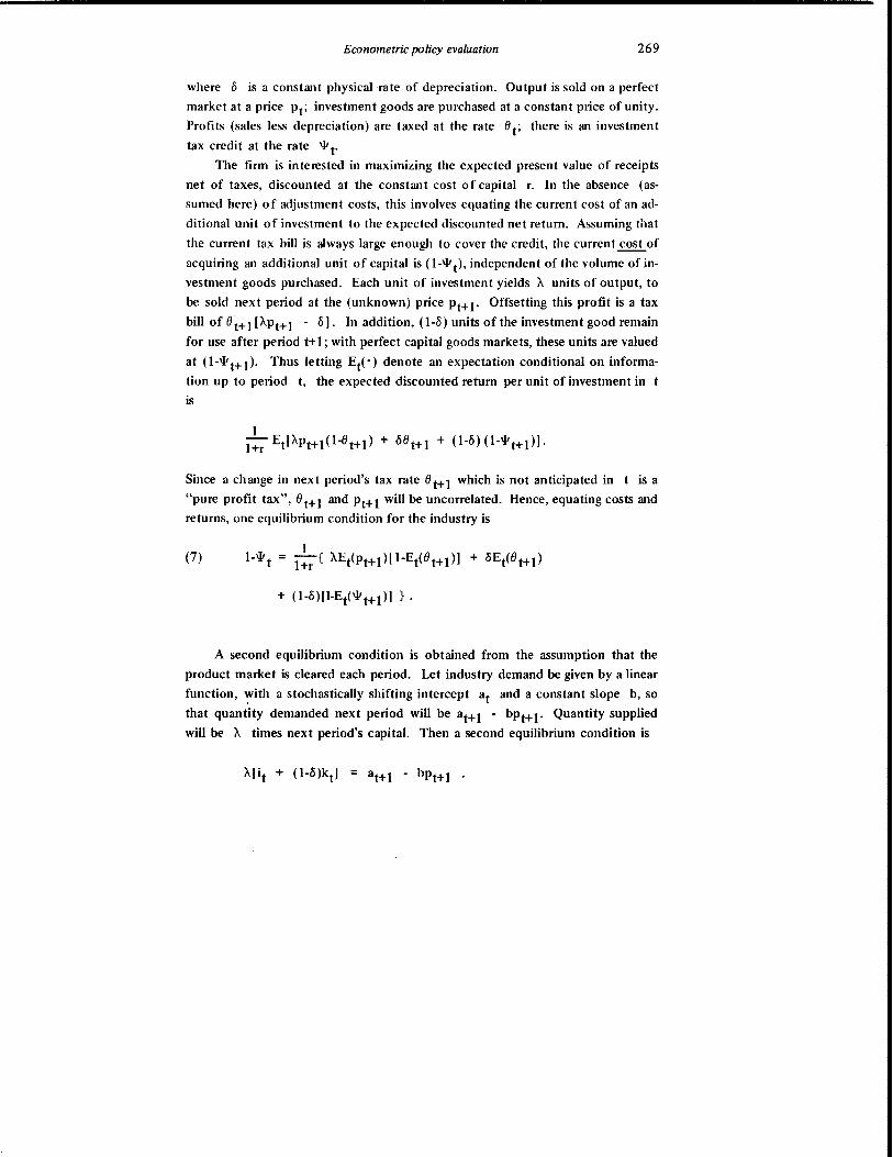
where 8 is a constant physical rate of depreciation. Output is sold on a perfect
market at a price Pt; investment goods are purchased at a constant price of unity.
Profits (sales less depreciation) are taxed at the rate 6 t; there is an investment
tax credit at the rate '11 t.
The firm is interested in maximizing the expected present value of receipts
net of taxes, discounted at the constant cost of capital r. In the absence (as
sumed here) of adjustment costs, this involves equating the current cost of an ad
ditional unit of investment to the expected discounted net return. Assuming that
the current tax bill is always large enough to cover the credit, the current cost of
acquiring an additional unit of capital is (1-'11 t), independent of the volume of in
vestment goods purchased. Each unit of investment yields A units of output, to
be sold next period at the (unknown) price Pt+ 1. Offsetting this profit is a tax
bill of 6t+1 [/'Pt+l - 8]. In addition, (1-8) units of the investment good remain
for use after period t+ 1; with perfect capital goods markets, these units are valued
at (1-'11 t+ 1). Thus letting Et(·) denote an expectation conditional on informa
tion up to period t, the expected discounted return per unit of investment in t
is
Since a change in next period's tax rate 6 t+1 which is not anticipated in t is a
"pure profit tax", 6t+l and Pt+l will be uncorrelated. Hence, equating costs and
returns, one equilibrium condition for the industry is
(7)
A second equilibrium condition is obtained from the assumption that the
product market is cleared each period. Let industry demand be given by a linear
function, ~ith a stochastically shifting intercept at and a constant slope b, so
that quantity demanded next period will be at+ 1 - bPt+ 1. Quantity supplied
will be A times next period's capital. Then a second equilibrium condition is

270 R.E. Lucas, Jr.
Taking mean values of both sides,
(8)
Since our interest is in the industry investment function, we eliminate
Et(pt+ I) between (7) and (8) to obtain:
(9) it (l-cS)kt+1 1 l [ r + cS] + };: Et(at+ 1)
A2 l-Et (8 t+1)
b (1 +r)\}I t - (1-cS )Et(\}I t+ 1) +
A2 [ 1 ]
Et(8 t+ 1)
Equation (9) gives the industry's "desired" stock of capital, it + (1-cS )kt, as a
function of the expected future state of demand and the current and expected
future tax structure, as well as of the cost of capital r, taken in this illustration
to be constant. The second and third terms on the right are the product of the
slope of the demand curve for capital, -bA-2, and the familiar Jorgensonian im
plicit rental price; the second term includes "interest" and depreciation costs,
net of taxes; the third includes the expected capital gain (orloss) due to changes
in the investment tax credit rate. In most empirical investment studies, firms are assumed to move gradually
from kt to the desired stock given by (9), due to costs of adjustment, delivery
lags, and the like. We assume here, purely for convenience, that the full adjust
ment occurs in a single period. Equation (9) is operationally at the same level as equations (1) and (4) of
the preceding section: it relates current behavior to unobserved expectations of
future variables. To move to a testable hypothesis, one must specify the time
series behavior of at, 8t and \}It (as was done for income in consumption theory),
obtain the optimal forecasting rule, and obtain the analogue to the consumption
function (6). Let us imagine that this has been accomplished, and estimates of
the parameters A and b have been obtained. How would one use these esti
mates to evaluate the consequences of a particular investment tax credit policy?
The method used by Hall and J.?rgenson is to treat the credit as a permanent
or once-and-for-all change, or implicitly to set Et(\}I t+ I) equal to \}It· Holding
Econometric policy evaluation 271
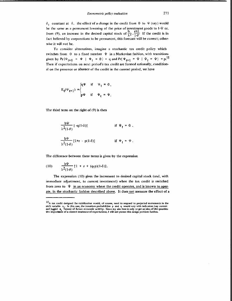
et constant at e, the effect of a change in the credit from 0 to \}t (say) would
be the same as a permanent lowering of the price of investment goods to l-\}t or,
from (9), an increase in the desired capital stock of ~2 • 7-:. If the credit is in
fact believed by corporations to be permanent, this forecast will be correct; other
wise it will not be.
To consider alternatives, imagine a stochastic tax credit policy which
switches from 0 to a fixed number \}t in a Markovian fashion, with transitions
given by pr{ \}t t+ 1 = \}t I \}t t = O} = q and Pr{ \}t t+ 1 = \}t I \}t t = \}t} = p.15
Then if expectations on next period's tax credit are formed rationally, condition
al on the presence or absence of the credit in the current period, we have
The third term on the right of (9) is then
b\}t -.:::..~ [ -q(1-o)] ,,20-e)
b\}t --[l+r - pO-8)] ,,20-8)
if \}t t 0,
if \}t t
The difference between these terms is given by the expression
(0) b\}t
-2-- [1 + r + (q-p)0-8)]. " (1-8)
The expression (l0) gives the increment to desired capital stock (and, with
immediate adjustment, to current investment) when the tax credit is switched
from zero to \}t in an economy where the credit operates, and is known to oper
ate, in the stochastic fashion described above. It does not measure the effect of a
15 A tax credit designed for stabilization would, of course, need to respond to projected movements in the shift variable at. In this case, the transition probabilities p and q would vary with indicators (say current and lagged at values) of future economic activity. Since my aim here is only to get an idea of the quantitative imporiance of a conect treatment of expectations, I will not pursue this design problem further.
272 R.E. Lucas, Jr.
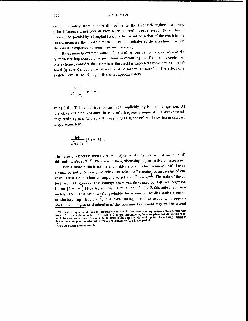
switch in policy from a no-credit regime to the stochastic regime used here.
(The difference arises because even when the credit is set at zero in the stochastic
regime, the possibility of capital loss,due to the introduction of the credit in the
future, increases the implicit rental on capital, relative to the situation in which
the credit is expected to remain at zero forever.) By examining extreme values of p and q one can get a good idea of the
quantitative importance of expectations in measuring the effect of the credit. At
one extreme, consider the case where the credit is expected almost never to be of
fered (q near 0), but once offered, it is permanent (p near 1). The effect of a
switch from 0 to 'l' is, in this case, approximately
b'l' [r + <'lJ,
using (10). This is the situation assumed, implicitly, by Hall and Jorgenson. At
the other extreme, consider the case of a frequently imposed but always transi
tory credit (q near 1, p near 0). Applying (10), the effect of a switch in this case
is approximately
b'l' ~~-[2+r-<'l] . ,,2(1-8)
The ratio of effects is then (2 + r - <'l )/(r + <'l). With r = .14 and <'l = .15, this ratio is about 7.1 6 We are not, then, discussing a quantitatively minor issue.
For a more realistic estimate, consider a credit which remains "off' for an
average period of 5 years, and when "switched on" remains for an average of one
year. These assumptions correspond to setting p;;;-'O and q=~. The ratio of the ef
fect (from (10»,under these assumptions versus those used by Hall and Jorgenson
is now [1 + r + ~ (1-<'l)] /(r+<'l). With r = .14 and <'l = .15, this ratio is approxi
mately 4.5. This ratio would probably be somewhat smaller under a more
satisfactory lag structure l7, but e~'en taking this into account, it appears
likely that the potential stimulus of the investment tax credit may well be several
16The cost of capital of .14 and the depreciation rate of .15 (for manufacturing equipment) are annual rates from [IS). Since the ratio (2 + r • O)/(r + <'l) is not time·unit free, the assumption that aU movement toward the new desired stock of capital takes place inone year is crucial at this point: by defining a period as shorter than one year this ratio wiU increase, and conversely for a longer period.
17For the reason given in note 16.

Econometric policy evaluation 273
times greater than the Hall-Jorgen"son estimates would indicate. 18
As was the case in the discussion of consumption behavior, estimation of a
policy effect along the above lines presupposes a policy generated by a fixed, rela
tively simple rule, known by forecasters (ourselves) and by the agents subject to
the policy (an assumption which is not only convenient analytically but consis
tent with Article I, Section 7 of the U.S. Constitution). To go beyond the kind
of order-of-magnitude calculations used here to an accurate assessment of the ef
fects of the 1962 credit studied by Hall and Jorgenson, one would have to infer
the implicit rule which generated (or was thought by corporations to generate)
that policy, a task made difficult, or perhaps impossible, by the novelty of the
policy at the time it was introduced. Similarly, there is no reason to hope that we
can accurately forecast the effects of future ad hoc tax policies on investment be
havior. On the other hand, there is every reason to believe that good quantitative
assessments of counter-cyclical fiscal rules, which are built into the tax structure
in a stable and well-understood way, can be obtained.
5.3 Phillips Curves
A third example is suggested by the recent controversy over the Phelps
Friedman hypothesis that permanent changes in the inflation rate will not alter
the average rate of unemployment. Most of the major econometric models have
been used in simulation experiments to test this proposition; the results are uni
formly negative. Since expectations are involved in an essential way in labor and
product market supply behavior, one would presume, on the basis of the consi
derations raised in section 4, that these tests are beside the point.19 This pre
sumption is correct, as the following example illustrates.
It will be helpful to utilize a simple, parametric model which captures the
main features of the expectational view of aggregate supply - rational agents,
cleared markets, incomplete information.20 We imagine suppliers of goods to be
distributed over N distinct markets i, i=l, ... ,N. To avoid index number problems,
suppose that the same (except for location) good is traded in each market, and
let Yit be the log of quantity supplied in market i in period t. Assume, further,
that the supply Yit is composed of two factors
1811 should be noted that this conclusion reinforces the qualitative conclusion reached by Hall and Jorgen· son [15), p. 413.
19Sargent [34) and I [23) have developed this conclusion earlier in similar contexts.
2<1rhis model is taken, with a few changes, from my earlier [24).

274 R.E. Lucas, Jr.
where yP denotes normal or permanent supply, and y~ cyclical or transitory rt rt
supply (both, again, in logs). We take yP to be unresponsive to all but permart
nent relative price changes or, since the latter have been defined away by assum-
ing a single good, simply unresponsive to price changes. Transitory supply y~ It varies with perceived changes in the relative price of goods in i:
where Pit is the log of the actual price in i at t, and p~ is the log of the genIt
eral (geometric average) price level in the economy as a whole, as perceived in
market i.21
Prices will vary from market to market for each t, due to the usual sources
of fluctuation in relative demands. They will also fluctuate over time, due to
movements in aggregate demand. We shall not explore the sources of these price
movements (although this is easy enough to do) but simply postulate that the ac
tual price in i at t consists of two components:
Pit = Pt + zit .
Sellers observe the actual price Pit; the two components cannot be separately
observed. The component Pt varies with time, but is common to all markets.
Based on information obtained prior to t (call it It-I) traders in all markets take
Pt to be a normally distributed random variable, with mean Pt (reflecting this
past information) and variance 0 2. The component Zit reflects relative price
variation across markets and time: Zit is normally distributed, independent of
Pt and z.s (unless i=j, s=t), with mean 0 and variance T2.
The ~ctual general price level at t is the average over markets of individual
prices,
N ~ Pit =
N i=1
1 Pt + N
N ~
i=1
We take the number of markets N to be large, so that the second term can be ne
glected, and Pt is the general price level. To form the supply decision, suppliers
estimate Pt; assume that this estimate p~ is the mean of the true conditional rt
21This supply function for goods should> be thought of as drawn up given a cleared labor market in i. See Lucas and Rapping (22) for an analysis of the factors underlying this function.
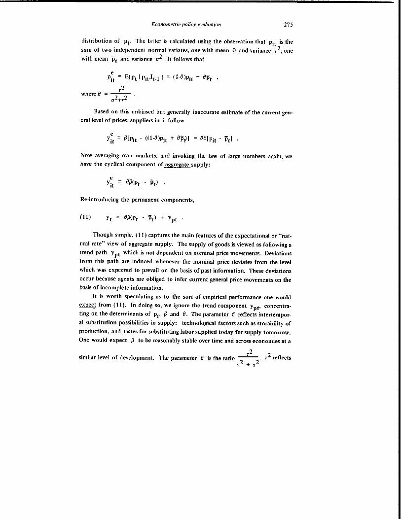
Econometric policy evaluation 275
distribution of Pt. The latter is calculated using the observation that Pit is the
sum of two independent normal variates, one with mean 0 and variance r2; one
with mean Pt and variance 02. It follows that
where 0
P~t = E{ Pt I Pith I } = (1-8 )Pit + OPt '
r2 ----
Based on this unbiased but generally inaccurate estimate of the current generallevel of prices, suppliers in i follow
Now averaging over markets, and invoking the law of large numbers again, we
have the cyclical component of aggregate supply:
Re-introducing the permanent components,
(11) Yt = O(3(Pt - Pt) + ypt .
Though simple, (II) captures the main features of the expectational or "nat
ural rate" view of aggregate supply. The supply of goods is viewed as following a
trend path ypt which is not dependent on nominal price movements. Deviations
from this path are induced whenever the nominal price deviates from the level
which was expected to prevail on the basis of past information. These deviations
occur because agents are obliged to infer current general price movements on the
basis of incomplete information.
It is worth speculating as to the sort of empirical performance one would
expect from (11). In doing so, we ignore the trend component ypt, concentra
ting on the determinants of Pt, (3 and O. The parameter (3 reflects intertempor
al substitution possibilities in supply: technological factors such as storability of
production, and tastes for substituting labor supplied today for supply tomorrow.
One would expect (3 to be reasonably stable over time and across economies at a
r2 2 similar level of development. The parameter 0 is the ratio -2---2. T reflects
o + T
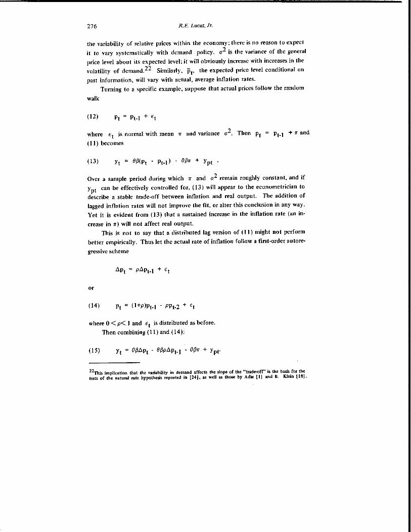
276 R.E. Lucas, Jr.
the variability of relative prices within the economy; there is no reason to expect
it to vary systematically with demand policy. a2 is the variance of the general
price level about its expected level; it will obviously increase with increases in the
volatility of demand.22 Similarly, Pt' the expected price level conditional on
past information, will vary with actual, average inflation rates.
Turning to a specific example, suppose that actual prices follow the random
walk
(12) Pt = Pt-I + Et
where Et is normal with mean 1T and variance a2. Then Pt
(I 1) becomes
(13) Yt = e{3(pt - Pt-I) - e{31T + ypt .
Pt-I + 1T and
Over a sample period during which 1T and a2 remain roughly constant, and if
ypt can be effectively controlled for, (13) will appear to the econometrician to
describe a stable trade-off between inflation and real output. The addition of
lagged inflation rates will not improve the fit, or alter this conclusion in any way.
Yet it is evident from (13) that a sustained increase in the inflation rate (an in
crease in 1T) will not affect real output.
This is not to say that a distributed lag version of (11) might not perform
better empirically. Thus let the actual rate of inflation follow a first-order autore
gressive scheme
or
(14) Pt = (1+P)Pt-l - PPt-2 + Et
where 0 < p< 1 and Et is distributed as before.
Then combining (11) and (14):
(15) y t = e{3.:lPt - e{3p.:lpt_1 - e{31T + ypt·
22This implication that the variability in demand affects the slope of the "trade-off' is the basis for the tests of the natural rate hypothesis reported in (24), as well as those by Adie (1) and B. Klein (18).
Econometric policy evaluation 277
In econometric terms, the "long-run" slope, or trade-off, would be the sum of the
inflation coefficients, or e!3( I-p), which will not, if (14) is stable, be zero.
In short, one can imagine situations in which empirical Phillips curves ex
hibit long lags and situations in which there are no lagged effects. In either case,
the "long-run" output-inflation relationship as calculated or simulated in the con
wmtional way has..!!2 bearing on the actual consequences of pursuing a policy of
inflation.
As in the consumption and investment examples, the ability to use (13) or
(15) to forecast the consequences of a change in policy rests crucially on the as
sumption that the parameters describing the new policy (in this case 7T, 0 2 and p)
are known by agents. Over periods for which this assumption is not approximate
ly valid (obviously there have been, and will continue to be, many such periods)
empirical Phillips curves will appear subject to "parameter drift," describable
over the sample period, but unpredictable for all but the very near future.
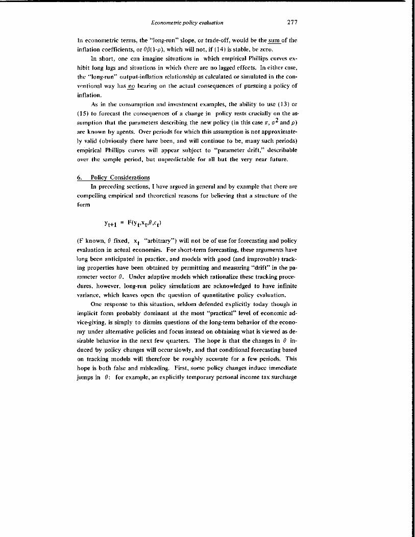
6. Policy Considerations
In preceding sections, I have argued in general and by example that there are
compelling empirical and theoretical reasons for believing that a structure of the
form
(F known, e fixed, Xt "arbitrary") will not be of use for forecasting and policy
evaluation in actual economies. For short-term forecasting, these arguments have
long been anticipated in practice, and models with good (and improvable) track
ing properties have been obtained by permitting and measuring "drift" in the pa
rameter vector e. Under adaptive models which rationalize these tracking proce
dures, however, long-run policy simuhitions are acknowledged to have infinite
variance, which leaves open the question of quantitative policy evaluation.
One response to this situation, seldom defended explicitly today though in
implicit form probably dominant at the most "practical" level of economic ad
vice-giving, is simply to dismiss questions of the long-term behavior of the econo
my under alternative policies and focus instead on obtaining what is viewed as de
sirable behavior in the next few quarters. The hope is that the changes in e in
duced by policy changes will occur slowly, and that conditional forecasting based
on tracking models will therefore be roughly accurate for a few periods. This
hope is both false and misleading. First, some policy changes induce immediate
jumps in e: for example, an explicitly temporary personal income tax surcharge
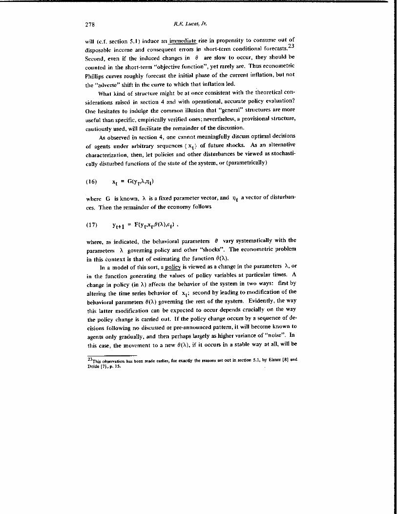
278 R.E. Lucas, Jr.
will (c.f. section 5.1) induce an immediate rise in propensity to consume out of
disposable income and consequent errors in short-term conditional forecasts. 23
Second, even if the induced changes in fJ are slow to occur, they should be
counted in the short-term "objective function", yet rarely are. Thus econometric
Phillips curves roughly forecast the initial phase of the current inflation, but not
the "adverse" shift in the curve to which that inflation led. What kind of structure might be at once consistent with the theoretical con
siderations raised in section 4 and with operational, accurate policy evaluation?
One hesitates to indulge the common illusion that "general" structures are more
useful than specific, empirically verified ones; nevertheless, a provisional structure,
cautiously used, will facilitate the remainder of the discussion.
As observed in section 4, one cannot meaningfully discuss optimal decisions
of agents under arbitrary sequences {Xt} of future shocks. As an alternative
characterization, then, let policies and other disturbances be viewed as stochasti
cally disturbed functions of the state of the system, or (parametrically)
where G is known, A is a fixed parameter vector, and 1It a vector of disturban
ces. Then the remainder of the economy follows
where, as indicated, the behavioral parameters fJ vary systematically with the
parameters A governing policy and other "shocks". The econometric problem
in this context is that of estimating the function fJ(A).
In a model of this sort, a policy is viewed as a change in the parameters A, or
in the function generating the values of policy variables at particular times. A
change in policy (in A) affects the behavior of the system in two ways: first by
altering the time series behavior of Xt; second by leading to modification of the
behavioral parameters fJ(A) governing the rest of the system. Evidently, the way
this latter modification can be expected to occur depends crucially on the way
the policy change is carried out. If the policy change occurs by a sequence of de
cisions following no discussed or pre-announced pattern, it will become known to
agents only gradually, and then perhaps largely as higher variance of "noise". In
this case, the movement to a new 8(1..), if it occurs in a stable way at all, will be
23This observation has been made earlier, for exactly the reasons set out in section 5.1, by Eisner [81 and Dolde [7\, p. IS.
Econometric policy evaluation 279
unsystematic, and econometrically unpredictable. If, on the other hand, policy
changes occur as fully discussed and understood changes in rules, there is some
hope that the resulting structural changes can be forecast on the basis of estima
tion from past data of OCA).
It is perhaps necessary to emphasize that this point of view towards condi
tional forecasting, due originally to Knight and, in modern fornl, to Muth, does
not attribute to agents unnatural powers of instantly divining the true structure of
policies affecting them. More modestly, it asserts that agents' responses become
predictable to outside observers only when there can be some confidence that
agents and observers share a common view of the nature of the shocks which
must be forecast by both.
The preference for "rules versus authority" in economic policy making sug
gested by this point of view, is not, as I hope is clear, based on any demonstrable
optimality properties of rules-in- general (whatever that might mean). There seems
to be no theoretical argument ruling out the possibility that (for example) dele
gating economic decision-making authority to some individual or group might
not lead to superior (by some criterion) economic performance than is attainable
under some, or all, hypothetical rules in the sense of (16). The point is rather
that this possibility cannot in principle be substantiated empirically. The only
scientific quantitative policy evaluations available to us are comparisons of the
consequences of alternative policy rules.
7. Concluding Remarks
This essay has been devoted to an exposition and elaboration of a single syl
logism: given that the structure of an econometric model consists of optimal de
cision rules of economic agents, and that optimal decision rules vary systematical
ly with changes in the structure of series relevant to the decision maker, it follows
that any change in policy will systematically alter the structure of econometric
models.
For the question of the short-term forecasting, or tracking ability of econo
metric models, we have seen that this conclusion is of only occasional significance.
For issues involving policy evaluation, in contrast, it is fundamental; for it implies
that comparisons of the effects of alternative policy rules using current macro
econometric models are invalid regardless of the performance of these models
over the sample period or in ex ante short-term forecasting.
The argument is, in part, destructive: the ability to forecast the consequen
ces of "arbitrary", unannounced sequences of policy decisions, currently claimed
(at least implicitly) by the theory of economic policy, appears to be beyond the

280 R.E. Lucas, Jr.
capability not only of the current-generation models, but of conceivable future
models as well. On the other hand, as the consumption example shows, condi
tional forecasting under the alternative structure (16) and (17) is, while scientif
ically more demanding, entirely operational.
In short, it appears that policy makers, if they wish to forecast the response
of citizens, must take the latter into their confidence. This conclusion, if iII
suited to current econometric practice, seems to accord well with a preferellce
for democratic decision making.
Econometric policy evaluation 281
REFERENCES
I. Adie, Douglas K., "The Importance of Expectations for the Phillips Curve
Relation," Research Paper No. 133, Department of Economics, Ohio Univer
sity (undated).
2. Ando, Albert and Franco Modigliani, "The Life Cycle Hypothesis of Saving;
Aggregate Implications and Tests," American Economic Review, v. 53
(1963), pp. 55-84.
3. Cooley, Thomas F. and Edward C. Prescott, "An Adaptive Regression Mo
del," International Economic Review, (June 1973),364-71.
4. , "Tests of the Adaptive Regression Model," Review
of Economics and Statistics, (April 1973), 248-56.
5. , "Estimation in the Presence of Sequential Parameter
Variation," Econometrica, forthcoming.
6. de Menil, George and Jared J. Enzler, "Prices and Wages in the FRB-MIT-Penn
Econometric Model," in Otto Eckstein, ed., The Econometrics of Price De
termination Conference (Washington: Board of Governors of the Federal
Reserve System and Social Science Research Council), 1972, pp. 277-308.
7. Dolde, Walter, "Capital Markets and the Relevant Horizon for Consumption
Planning," Yale doctoral dissertation, 1973.
8. Eisner, Robert, "Fiscal and Monetary Policy Reconsidered," American Eco
nomic Review, v. 59 (1969), pp. 897-905.
9. Evans, Michael K. and Lawrence R. Klein, The Wharton Econometric Fore
casting Model. 2nd, Enlarged Edition (Philadelphia: University of Pennsyl
vania Economics Research Unit), 1968.
10. Fisher, Franklin M., "Discussion" in Otto Eckstein, ed., op. cit. (reference
(6)), pp. 113-115.
11. Friedman, Milton, A Theory of the Consumption Function. (Princeton:
Princeton University Press), 1957.
282
12.
13.
R. E. Lucas, Jr.
-------, "Windfalls, the 'Horizon', and Related Concepts in the
Permanent Income Hypothesis," in Carl F. Christ, et. aI., eds., Measurement
in Economics (Stanford: Stanford University Press), 1963, pp. 3-28.
-------, "The Role of Monetary Policy," American Economic Review, v. 58 (1968), pp. 1-17.
14. Gordon, Robert J., "Wage-Price Controls and the Shifting Phillips Curve,"
Brookings Papers on Economic Activity, 1972, no. 2, pp. 385-421.
IS. Hall, Robert E. and Dale W. Jorgenson, "Tax Policy and Investment Behav
ior," American Economic Review; v. 57 (1967), pp. 391-414.
16. Hirsch, Albert A., "Price Simulations with the OBE Econometric Model," in Otto Eckstein, ed., op.cit. (reference [6) ), pp. 237-276.
17. Hymans, Saul H., "Prices and Price Behavior in Three U.S. Econometric
Models," in Otto Eckstein, ed., op. cit. (reference [6), pp. 309-322.
18. Klein, Benjamin, "The Effect of Price Level Unpredictability on the Compo
sition oflncome Change," unpublished working paper, April, 1973.
19. Klein, Lawrence R. and Arthur S. Goldberger, An Econometric Model of the
United States, 1929-1952.(Amsterdam: North Holland), 1955.
20. Klein, Lawrence R., An Essay on the Theory of Economic Prediction.(Helsinki: Yrjo Jahnsson Lectures), 1968.
21. Knight, Frank H., Risk, Uncertainty and Profit.(Boston: Houghton-Mifflin), 1921.
22. Lucas, Robert E., Jr. and Leonard A. Rapping, "Real Wages, Employment,
and Inflation," Journal of Political Economy, v. 77 (1969), pp. 721-754.
23. Lucas, Robert E.,Jr., "Econometric Testing of the Natural Rate Hypothesis,"
in Otto Eckstein, ed., op. cit. (reference [6) ), pp. 50-59.
24.
Econometric policy evaluation 283
-------, "Some International Evidence on Output-Inflation Trade- Offs," American Economic Review, v. 63 (1973).
25. Marschak, Jacob, "Economic Measurements for Policy and Prediction," in
William C. Hood and Tjalling G. Koopmans, eds., Studies in Econometric
Method, Cowles Commission Monograph 14 (New York: Wiley), 1953, pp. 1-26.
26. Mayer, Thomas, "Tests of the Permanent Income Theory with Continuous
Budgets," Journal of Money, Credit, and Banking, v. 4 (1972)pp. 757-778.
27. Modigliani, Franco and Richard Brumberg, "Utility Analysis and the Con
sumption Function: An Interpretation of Cross-Section Data," in K. K.
Kurihara, ed., Post-Keynesian Economics.(New Brunswick: Rutgers University Press), 1954.
28. Muth, John F., "Optimal Properties of Exponentially Weighted Forecasts,"
Journal of the American Statistical Association, v. 55 (1960), pp. 299-306.
29. , "Rational Expectations and the Theory of Price Move-
ments," Econometrica, v. 29 (1961), pp. 315-335.
30. Phelps, Edmund S., "Money Wage Dynamics and Labor Market Equilibrium,"
Journal of Political Economy, v. 76 (1968), pp. 687-711.
31. Phelps, Edmund S., et aI., The New Microeconomics in Employment and In
flation Theory.(New York: Norton), 1970.
32. Phillips, A. W., "The Relation Between Unemployment and the Rate of
Change of Money Wage Rates in the United Kingdom, 1861-1957," Econo
mica, v. 25 (1958), pp. 283-299.
33. Samuelson, Paul A. and Robert M. Solow, "Analytical Aspects of Anti-In
flation Policy," American Economic Review, v. 50 (1960), pp. 177-194.
34. Sargent, Thomas J., "A Note on the 'Accelerationist' Controversy," ~
of Money, Credit, and Banking, v. 3 (1971), pp. 721-725.

284 R.E. Lucas, Jr.
35. Tinbergen, Jan, On the Theory of Economic Policy. (Amsterdam: North
Holland), 1952.
36. , Economic Policy: Principles and Design. (Amsterdam:
North Holland), 1956.