Econometrics: Computer Modellingfelixpretis.climateeconometrics.org/wp-content/uploads/...Batch Code Using Batch Code, estimate and store the following models for Gradschool admissions:

Would you have survived the sinking of the Titanic?

Felix Pretis (Oxford) Econometrics Oxford University, 2016 1 / 38

Introduction

Econometrics: Computer Modelling

Felix Pretis

Programme for Economic ModellingOxford Martin School, University of Oxford

Lecture 2: Micro-Econometrics:Limited Dep. Variable Models


Structure

1: Intro to Econometric Software & Cross-Section Regression

2: Micro-Econometrics: Limited Indep. Variable

3: Macro-Econometrics: Time Series


Aim of this Course

Last time:Introduce econometric modelling in practiceIntroduce OxMetrics/PcGive Software

Today:Binary dependent variables & Count data

Probability of being accepted into a Masters/PhD Programme(between [0,1])Number of arrests (count)Prob. of surviving the Titanic sinking, participating in labour force

Additional functions in OxMetrics/PcGive


Motivation

Economies high dimensional, interdependent, heterogeneous,and evolving: comprehensive specification of all events isimpossible.Economic Theory

likely wrong and incompletemeaningless without empirical support

Econometrics to discover new relationships from dataEconometrics can provide empirical support. . . or refutation.


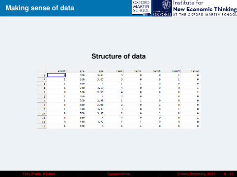
Making sense of data

Structure of data


Gradschool Admissions

Data on admission to graduate school (US) as a function of:

GPA

GRE score

Rank of undergraduate institution

Dataset: ”gradschool.xlsx”

Other file formats? Datasets: .in7 & .bn7 files


Task

Build a Linear Probability Model (LPM) for gradschool admission:

Create a new database in OxMetricsGo to File, New, OxMetrics DataSet start period = 1 (undated for cross-sectional data)Copy & Paste Data from Excel file: ”gradschool.xlsx”Save as .in7 data file on your computer

Or open .csv in OxMetricsConstruct appropriate variables to take the rank of the universityinto account

Algebra: rank1 = (rank == 1) ? 1 : 0;creates a dummy variable = 1 if rank==1

Plot the observed and predicted values against GRE. Based onthe model output highlight shortcomings of the LPM


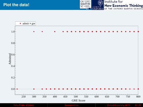
Plot the data!

admit × gre

250 300 350 400 450 500 550 600 650 700 750 800

0.0

0.2

0.4

0.6

0.8

1.0

Adm

itted

GRE Score

admit × gre


Linear Probability Model

Fit a simple Linear probability model (OLS)EQ( 1) Modelling admit by OLS-CS

The dataset is: gradschool.in7The estimation sample is: 1 - 400

Coefficient Std.Error t-value t-prob Part.Rˆ2Constant -0.258910 0.2160 -1.20 0.2314 0.0036gre 0.000429572 0.0002107 2.04 0.0422 0.0104gpa 0.155535 0.06396 2.43 0.0155 0.0148rank2 -0.162365 0.06771 -2.40 0.0170 0.0144rank3 -0.290570 0.07025 -4.14 0.0000 0.0416rank4 -0.323026 0.07932 -4.07 0.0001 0.0404

sigma 0.444866 RSS 77.9750245Rˆ2 0.100401 F(5,394) = 8.795 [0.000]**Adj.Rˆ2 0.0889844 log-likelihood -240.56no. of observations 400 no. of parameters 6mean(admit) 0.3175 se(admit) 0.466087

Normality test: Chiˆ2(2) = 212.46 [0.0000]**Hetero test: F(7,392) = 3.8513 [0.0005]**Hetero-X test: F(8,391) = 3.6183 [0.0004]**RESET23 test: F(2,392) = 0.19773 [0.8207]


Linear Probability Model

Concerns with Linear Probability Model

Assumes continuous dep. variable & constant effect of covariateson probability of success (could exceed 1)

Predicted values outside [0,1] range: Test - Store...

Heteroskedasticity by construction:

P(y = 1|x) = x ′β+ u (1)

V(u|x) = x ′β(1− x ′β) (2)


Fitted Values of LPM

admit × gre LPM_fitted × gre

250 300 350 400 450 500 550 600 650 700 750 800

0.0

0.2

0.4

0.6

0.8

1.0

Adm

itted

GRE





250 300 350 400 450 500 550 600 650 700 750 800

0.0

0.2

0.4

0.6

0.8

1.0

Adm

itted

GRE



Logistic Regression Model

Binary response variable, link function G(·)

P(y = 1|x) = G(β0 + β1x1 + · · ·+ βkxk) = G(β0 + xβ) (3)

Probit:P(y = 1|x) = Φ(x ′β) (4)

Φ(·) is the standard normal distribution function.

Logistic Regression:

P(y = 1|x) =exp (β0 + xβ)

1+ exp (β0 + xβ)(5)

Maximum Likelihood Estimation

No analytical solution


Logit: Interpretation of β

1) Log-Odds Ratio

Note that the odds ratio (probability of success over probability offailure) in the logit model is given as:

P(y = 1|x)

1− P(y = 1|x)= exp(β0 + xβ) (6)

Therefore, taking logs:

log

(P(y = 1|x)

1− P(y = 1|x)

)= β0 + xβ (7)

Thus, 100× βk has the interpretation as % increase in odds ratio for aone-unit increase in xk


Logit: Interpretation of β

2) Marginal Effects (ME)

∂P(y = 1|x)

∂xk=

∂

∂xk

(exp (β0 + xβ)

1+ exp (β0 + xβ)

)(8)

= βkP(y = 1|x) (1− P(y = 1|x)) (9)

MEk same sign as coefficient βkMarginal effects are largest when P = 0.5, i.e. largest forindividuals whose outcomes have the highest variance, p(1− p).


Marginal Effects: Intuition

goo.gl/LUD7ftFelix Pretis (Oxford) Econometrics Oxford University, 2016 17 / 38

goo.gl/LUD7ft

Logistic Regression in OxMetrics

Models for Discrete Data

Binary Discrete Choice using PcGive

Logit

Newton’s Method (no analytical solution – numerical algorithm)

What are the effects of rank, gpa, gre, on the probability of beingadmitted to Grad School?


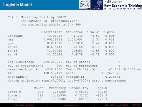
Logistic Model

CS( 1) Modelling admit by LOGITThe dataset is: gradschool.in7The estimation sample is 1 - 400

Coefficient Std.Error t-value t-probConstant -3.98998 1.140 -3.50 0.001gre 0.00226443 0.001094 2.07 0.039gpa 0.804038 0.3318 2.42 0.016rank2 -0.675443 0.3165 -2.13 0.033rank3 -1.34020 0.3453 -3.88 0.000rank4 -1.55146 0.4178 -3.71 0.000

log-likelihood -229.258746 no. of states 2no. of observations 400 no. of parameters 6baseline log-lik -249.9883 Test: Chiˆ2( 5) 41.459 [0.0000]**AIC 470.517492 AIC/n 1.17629373mean(admit) 0.3175 var(admit) 0.216694Newton estimation (eps1=0.0001; eps2=0.005): Strong convergence

Count Frequency Probability loglikState 0 273 0.68250 0.68250 -97.40State 1 127 0.31750 0.31750 -131.9Total 400 1.00000 1.00000 -229.3




250 300 350 400 450 500 550 600 650 700 750 800

0.0

0.2

0.4

0.6

0.8

1.0

Adm

itted

GRE



Fitted Values of Logistic

admit × gre Logistic_fitted × gre

LPM_fitted × gre

250 300 350 400 450 500 550 600 650 700 750 800

0.0

0.2

0.4

0.6

0.8

1.0

Adm

itted

GRE

admit × gre Logistic_fitted × gre

LPM_fitted × gre


Code in OxMetrics

Replicability is important!

Easy to make mistakes/forget what you have done. Code to reproduceyour modelling:

Batch code (intuitive code, similar to STATA do-files)

Ox code (matrix programming language, similar to Matlab, R)

Batch Code:

.fl files

ALT+B: Batch code for last model


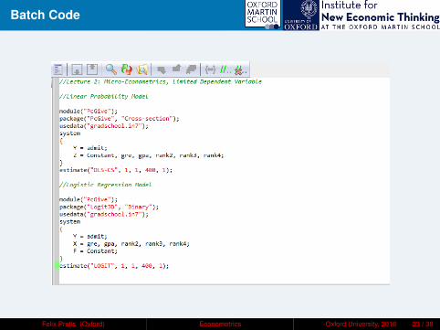
Batch Code


Batch Code

Using Batch Code, estimate and store the following models forGradschool admissions:

1 A linear probability model without an intercept with a differentbase rank

2 A logistic regression without GPA variable and using observationsfor the individuals i = 50, ..., 200.

3 In the form of comments in batch code, add the results of a testthat all rank variables can be dropped from the model.


Relating LPM to Logit Model

Estimate:

LPM of admit on constant and rank1

Logit Model of admit on constant and rank1

Compare predicted values.


Relating LPM to Logit Model

LPM of admit:The estimation sample is: 1 - 400

Coefficient Std.Error t-value t-prob Part.Rˆ2Constant 0.277286 0.02481 11.2 0.0000 0.2388rank1 0.263697 0.06354 4.15 0.0000 0.0415

Predicted: 0.277+ 0.26I{Rank=1}= 0.54 (for Rank = 1)

Logit of admit:Coefficient Std.Error t-value t-prob

Constant -0.957963 0.1213 -7.90 0.000rank1 1.12227 0.2841 3.95 0.000

Predicted:exp(−0.957+1.12I{Rank=1})

(1−exp(−0.957+1.12I{Rank=1}))

= 0.277 (for Rank 6= 1) and = 0.54 (for Rank = 1)


Count-data

So far: Binary dependent variable [0,1]Now: Count data – Poisson regression


Poisson Regression

Dependent Variable: non-negative integers 0,1,2...

y ∼ Poisson(µ)

linear model not ideal (as before)

Model expected value as exponential function:

E[yi|x] = exp(β0 + β1x1,i + · · ·+ βkxk,i) (10)

yi = E[yi|xi] + ui (11)

yi = ex ′iβ + ui (12)

Interpretation:

Approx: 100βk∆xk ≈ %∆E[yi|x]

Exact proportional change: exp(βk∆xk) − 1


Poisson Model: Estimation

Count data: 0, 1, 2, . . . , modelled as Poisson Distribution with λi:

E[yi|x] = λi = exp(β0 + β1x1,i + · · ·+ βkxk,i)V[yi|x] = E[yi|x]

P (Y = yi|λi(xi)) =e−λiλ

yii

yi!

Estimation using Maximum Likelihood.


Poisson Regression in OxMetrics

Modelling Number of Arrests:

Number of times a man is arrested in 1986: ‘narr86’

”arrests.in7”

Plot the data!


Poisson Regression in OxMetrics

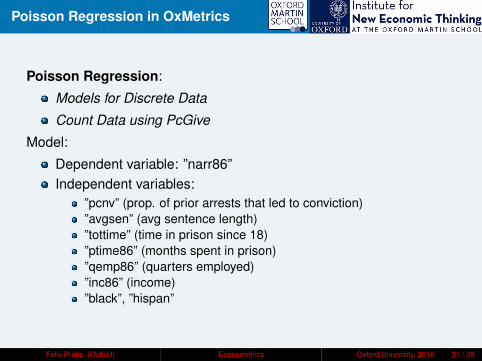
Poisson Regression:

Models for Discrete Data

Count Data using PcGive

Model:

Dependent variable: ”narr86”Independent variables:

”pcnv” (prop. of prior arrests that led to conviction)”avgsen” (avg sentence length)”tottime” (time in prison since 18)”ptime86” (months spent in prison)”qemp86” (quarters employed)”inc86” (income)”black”, ”hispan”


Poisson Output

CS( 1) Modelling narr86 by POISSONThe dataset is: arrests.in7The estimation sample is 1 - 2725

Coefficient Std.Error t-value t-probConstant -0.617178 0.06365 -9.70 0.000pcnv -0.405258 0.08488 -4.77 0.000avgsen -0.0236365 0.01993 -1.19 0.236tottime 0.0243425 0.01476 1.65 0.099ptime86 -0.0985944 0.02071 -4.76 0.000qemp86 -0.0361131 0.02892 -1.25 0.212inc86 -0.00814627 0.001038 -7.85 0.000black 0.660356 0.07383 8.94 0.000hispan 0.499594 0.07392 6.76 0.000

log-likelihood -2249.08013 not truncatedno. of observations 2725 no. of parameters 9baseline log-lik -2441.921 Test: Chiˆ2( 8) 385.68 [0.0000]**AIC 4516.16026 AIC/n 1.65730652mean(narr86) 0.404404 var(narr86) 0.737742


Number of arrests model

Store the batch code as ”.fl” file.

1 What is the effect of being black/hispanic on the number ofarrests?

2 Manually conduct a likelihood ratio test of: excluding black, hispan

Run Models in batch file.

LR = −2[ln(L̂R

)− ln

(L̂UR

)]∼ χ2q

χ22: 5% Critical value is 5.99


Task: Titanic Survival

Surviving the TitanicWhat is your estimated probability of survival?



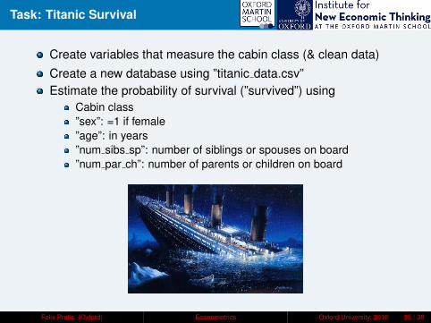
Create variables that measure the cabin class (& clean data)Create a new database using ”titanic data.csv”Estimate the probability of survival (”survived”) using

Cabin class”sex”: =1 if female”age”: in years”num sibs sp”: number of siblings or spouses on board”num par ch”: number of parents or children on board



Answering the following questions:1 What is the unconditional probability of survival?2 What is the average survival rate for each class?3 Estimate the following models using three alternative methods

and compare the resultsCreate batch file for your models & plots illustrating your results.What is the effect of cabin class/sex/age/having siblings or kidson-board on the probability of survival? How can the coefficientsbe interpreted? What difference do you find between the twomethods used?What is your personal probability of survival for your assignedcabin class, given that you assume your parents were not onboard, but your siblings/spouses (if you have any) would havebeen?

4 What determines the number of siblings people had on board?Construct a test for class not affecting the number of siblings.


Tasks 2: Female labour force

OxMetrics and PcGive Exercise: Female labour force participation.

Create a new database using ”labourforce.xlsx””inlf” binary variable =1 if married woman in labour force in 1975.

hours hours worked, 1975kidslt6 # kids < 6 yearskidsge6 # kids 6-18age woman’s age in yrseduc years of schoolingwage estimated wage from earns., hoursrepwage reported wage at interview in 1976hushrs hours worked by husband, 1975husage husband’s agehuseduc husband’s years of schoolinghuswage husband’s hourly wage, 1975faminc family income, 1975mtr fed. marginal tax rate facing womanmotheduc mother’s years of schoolingfatheduc father’s years of schoolingunem unem. rate in county of resid.city =1 if live in cityexper actual labor mkt exper


Tasks

Answering the following questions:

1 Estimate models using two alternative methods and compare the results(create a batch file).

2 What is the effect of age/educ/experience/having kids on the probabilityof being in the labour force? What difference do you find between thetwo methods used?

3 Allow for diminishing marginal returns to experience. What are yourfindings?

4 Build a more general model, including additional covariates. Which onesare significant? How could you reduce the number of variables?

5 Using batch code, sequentially eliminate variables based on theirsignificance (conduct backwards-elimination). What other modelselection methods could you use? Advantages/disadvantages?

6 Classification: Hold back 200 observations, predict the labour forceparticipation for the hold-back sample. What proportion are correctlyclassified? Build a model that achieves the highest classification rate.


Documents

Econometrics: Computer Modellingfelixpretis.climateeconometrics.org/wp-content/uploads/...Batch Code Using Batch Code, estimate and store the following models for Gradschool admissions: