Embed Size (px)
Citation preview
Econometrics of Survey Data
Manuel Arellano
CEMFI
September 2014
1

Introduction
• Suppose that a population is stratified by groups to guarantee that there will beenough observations to permit suffi ciently precise estimates for each of the groups.For example, these groups can be locations, age intervals, or wealth levels.
• Next, each subpopulation or stratum is divided into spatial clusters of households(apartment compounds, villages) and a random sample of clusters is selected fromeach stratum. Finally, a small number of households is selected at random withineach cluster.
• In general, sampling clusters is more cost effective than sampling households directly,despite the fact that individual observations within a cluster will likely be correlatedand therefore less informative than observations from individuals sampled at random.
• The above describes a prototypical multistage survey design in which bothstratification and clustering are present.
• We wish to discuss the implications of using this type of data for an econometricanalysis where the interest is in drawing conclusions about the original population.The econometric analysis could be of a descriptive nature (decomposition analysis orhedonic price indexes) or aim for non-structural or structural causal inference.
2
Introduction (continued)
• It is also of interest to think of complex survey designs in a figurative sense.
• Sometimes we wish to do statistical analysis of data which have not come to us as aresult of actual sampling. In those situations we implicitly decide the abstractpopulation of interest by imagining a sampling design that could have produced thedata at hand from such population.
• This is the case when we work with the universe of firms of certain characteristics orwhen we work with cross-sectional or longitudinal data on countries.
• At a more general level, the question of inference is: how much confidence can I havethat the pattern I see in the data is typical of some larger population, or that theapparent pattern is not only a random occurrence?
• From this perspective there is a role for inferential statistics as long as it can beanticipated that estimation error is not negligible relative to some conceptualpopulation of interest.
3

Outline
• Introduction• Finite populations
• Part 1: Weighted estimation and stratification• Weighted means and estimating equations• Standard errors under stratification• Examples: OLS, IV, QR, ML, subpopulations• Endogenous and exogenous stratification• Population heterogeneity vs sample design• Choice-based sampling
• Part 2: Cluster standard errors• Introduction• Cluster fixed-effects vs cluster standard errors• General set up: estimating equations• Examples: panel data, quantile regression
• Part 3: Bootstrap methods• The idea of the bootstrap• Bootstrap standard errors• Asymptotic properties• Bootstrapping stratified clustered samples• Using replicate weights
4
Finite populations
• Inference in microeconometrics typically assumes that data are generated as a randomsample with replacement or that is coming from an infinite population.
• These assumptions are not literally valid in the case of survey data that come from afinite population of units.
• There is an extensive literature in statistics dealing with the sampling schemes thatarise in survey production (e.g. Levy and Lemeshow 1991).
Random sampling without replacement• Consider a finite population N and the population mean given by
θ0 =1
N
N
∑i=1
Yi .
• Also define the following population variance
S2 =1
N − 1
N
∑i=1(Yi − θ0)
2 =1
N − 1Y ′QNY ,
where QN = I − ιι′/N is the deviation from means operator of order N .
• The Y =(Y1, ...,YN
)′ represent a full enumeration of the values of the variable andare therefore nonstochastic quantities.
5
Finite populations (continued)
• Let y1, ..., yN be a random sample of size N without replacement and sample mean:
Y =1N
N
∑j=1
yj
• The sample mean can be rewritten as a random selection of population values
Y =1N
N
∑i=1
aiYi
where ai is an indicator that takes the value 1 if i is in the sample, and 0 otherwise.
• Letting f = N/N , under random sampling
E (ai ) = f
Var (ai ) = f (1− f )
Cov(ai , aj
)= − 1(
N − 1) f (1− f ) ,
or in compact form,
Var (a) = f (1− f ) N(N − 1
)QN• The result uses that E
(aiaj
)= N
N(N−1)(N−1)
due to sampling without replacement.
6

Finite populations (continued)
• We immediately see that the sample mean is an unbiased estimator of the populationmean:
E(Y)=1N
N
∑i=1
E (ai )Yi =1N
N
∑i=1
N
NYi = θ0
• Moreover, the variance is given by
Var(Y)=
1N2Y ′Var (a)Y = (1− f ) S
2
N• The term 1− f is the finite population correction. When N → N the samplingvariance goes to zero, Var
(Y)→ 0.
• A multivariate generalization is straightforward.
• Typically, the population size is suffi ciently large relative to the sample size that1− f ≈ 1 and the correction can be ignored. This is the approach we’ll take in whatfollows.
• Standard asymptotic theory studies the properties of sample statistics from infinitepopulations as N → ∞.
• An alternative asymptotic framework to mimic situations where sample size is notnegligible relative to population size, is one in which both N and N tend to infinitywhile f tends to some positive fraction.
7
Finite populations (continued)
• An unbiased estimate of the population variance S2 is given by
s2 =1
N − 1N
∑i=1
(yi − Y
)2=
1N − 1 y
′QN y
• Ullah and Breunig (1998) show that E(s2)= S2. They also consider results for
linear regression and generalizations to stratified samples and clustering.
• It turns out that the OLS variance when sampling is without replacement is notnecessarily smaller than the infinite population OLS variance. The direction of theinequality depends upon the matrix of regressors.
• Moreover, it is possible to consider a GLS estimator that takes into account that errorsare not independent. Contrary to the mean model, GLS does not coincide with OLS.
8

Part 1: Weighted estimation and stratification
9
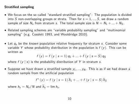
Stratified sampling
• We focus on the so called “standard stratified sampling”: The population is dividedinto S non-overlapping groups or strata. Then for s = 1, ...,S , we draw a randomsample of size Ns from stratum s . The total sample size is N = N1 + ...+NS .
• Related sampling schemes are “variable probability sampling” and “multinomialsampling” (e.g. Cosslett 1993, and Wooldridge 2010).
• Let qs be the known population relative frequency for stratum s . Consider somevariable Y whose probability distribution in the population is f (y ). This can bewritten as
f (y ) = f (y | s = 1) q1 + ...+ f (y | s = S) qSwhere f (y | s) is the probability distribution of Y in stratum s .
• Suppose we have drawn a stratified sample y1, ..., yN . This is as if we had drawn arandom sample from the artificial population
f ∗ (y ) = f (y | s = 1) h1 + ...+ f (y | s = S) hSwhere hs = Ns/N and hs = lim hs .
10
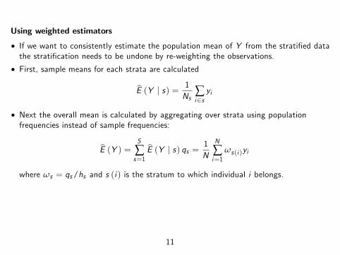
Using weighted estimators
• If we want to consistently estimate the population mean of Y from the stratified datathe stratification needs to be undone by re-weighting the observations.
• First, sample means for each strata are calculated
E (Y | s) = 1Ns
∑i∈syi
• Next the overall mean is calculated by aggregating over strata using populationfrequencies instead of sample frequencies:
E (Y ) =S
∑s=1
E (Y | s) qs =1N
N
∑i=1
ωs(i )yi
where ωs = qs/hs and s (i) is the stratum to which individual i belongs.
11

Weight factors
• The weight factor ωs(i ) is the ratio of the population share to the sample share.• It informs us that household i is representative of ωs(i )—times the number ofhouseholds it would represent in a random sample.
• Over-sampled categories are given a low weight, and vice-versa.• In a random sample ωs(i ) = 1 for all i , so that each unit in a sample of size N is
representative of N/N units in a population of size N (e.g. N/N = 2000 if N = 500and N = 1, 000, 000).
• For example, ωs(i ) = 3 means that unit i represents φi = ωs(i ) ×N/N = 6000comparable units.
• Weight factors add up to N :N
∑i=1
ωs(i ) = N1ω1 + ...+NSωS = q1N + ...+ qSN = N
Moreover, ∑Ni=1 φi = N .
• Using φi , E (Y ) can be seen as an approximate calculation of the population mean:
E (Y ) =1
N
N
∑i=1
φi yi .
• The φi are the standard definition of population weights in survey methodology.
12

Weighted estimating equations
• A generalization of the weighted mean in a GMM framework is as follows.
• Suppose we are interested in the estimation of some parameter θ0, which is acharacteristic of the possibly multivariate distribution f (w ) identified by the momentcondition
Eψ (W , θ0) = 0.
• In a stratified sample we would therefore expect
S
∑s=1
E [ψ (W , θ0) | s ] qs =1N
N
∑i=1
ωs(i )ψ (wi , θ0) ≈ 0
• So it is natural to estimate θ0 by θ, which precisely solves
1N
N
∑i=1
ωs(i )ψ(wi , θ
)= 0. (1)
• θ is a weighted generalized-method-of-moments (GMM) estimator.
• Here dim ψ = dim θ. If dim ψ > dim θ, θ will solve dim θ linear combinations of (1).
13

Asymptotic Variance
• Under standard regularity conditions the asymptotic variance of θ can be estimated as
H−1S
∑s=1
ω2s
[Ns
∑i∈s
(ψ(wi , θ
)− ψs
) (ψ(wi , θ
)− ψs
)′]H ′−1
where H = ∑Ni=1 ωs(i )∂ψ(wi ,θ)
∂θ′and ψs =
1Ns ∑Nsi∈s ψ
(wi , θ
).
• Means by strata need to be subtracted because in general E [ψ (W , θ0) | s ] 6= 0.
Example: Asymptotic variance of the weighted sample mean
• If ψ (wi , θ) = yi − θ, we get H = −∑Ni=1 ωs(i ) = −N and hence
1N2
S
∑s=1
ω2s
[Ns
∑i∈s(yi − y s )2
]=
S
∑s=1
N2sN2
ω2s
[1N2s
Ns
∑i∈s(yi − y s )2
]=
S
∑s=1
q2sσ2sNs
where
σ2s =1Ns
Ns
∑i∈s(yi − y s )2 .
• A suitable choice of h1, ..., hS will be variance reducing relative to random sampling.
14

Examples• The first example is linear regression:
ψ (wi , θ) = xi(yi − x ′i θ
)• Solving (1) we get the weighted-least squares estimator
θ =
(N
∑i=1
ωs(i )xi x′i
)−1 N
∑i=1
ωs(i )xi yi
• The second example is linear instrumental-variables :
ψ (wi , θ) = zi(yi − x ′i θ
)leading to
θ =
(N
∑i=1
ωs(i )zi x′i
)−1 N
∑i=1
ωs(i )zi yi .
• The third example is quantile regression:
ψ (wi , θ) = xi[1(yi ≤ x ′i θ
)− τ
].
In this case θ solves for τ ∈ (0, 1)
θ = arg minθ
N
∑i=1
ωs(i )ρτ
(yi − x ′i θ
)where ρτ (u) is the “check” function ρτ (u) = [τ1 (u ≥ 0) + (1− τ) 1 (u < 0)]× |u|.
15
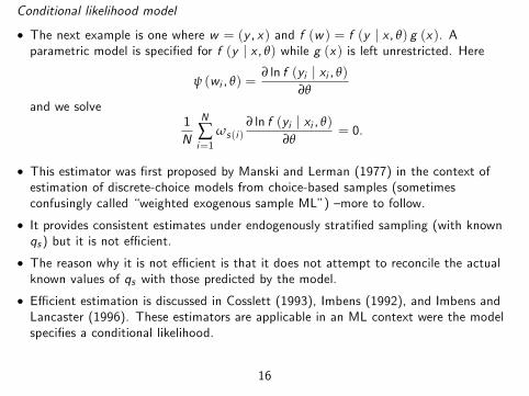
Conditional likelihood model
• The next example is one where w = (y , x) and f (w ) = f (y | x , θ) g (x). Aparametric model is specified for f (y | x , θ) while g (x) is left unrestricted. Here
ψ (wi , θ) =∂ ln f (yi | xi , θ)
∂θ
and we solve1N
N
∑i=1
ωs(i )∂ ln f (yi | xi , θ)
∂θ= 0.
• This estimator was first proposed by Manski and Lerman (1977) in the context ofestimation of discrete-choice models from choice-based samples (sometimesconfusingly called “weighted exogenous sample ML”) —more to follow.
• It provides consistent estimates under endogenously stratified sampling (with knownqs ) but it is not effi cient.
• The reason why it is not effi cient is that it does not attempt to reconcile the actualknown values of qs with those predicted by the model.
• Effi cient estimation is discussed in Cosslett (1993), Imbens (1992), and Imbens andLancaster (1996). These estimators are applicable in an ML context were the modelspecifies a conditional likelihood.
16

Estimating parameters from subpopulations
• In the last example interest is in estimating a characteristic θ0 of some subpopulation.• Let di indicate membership of the subpopulation and suppose that θ0 satisfies
E [ψ (wi , θ0) | di = 1] = 0
or equivalentlyE [ψ (wi , θ0) di ] = 0.
• Estimation is based on the sample moment
N
∑i=1
ωs(i )diψ(wi , θ
)= 0.
• For example, if interested in the mean of yi for the units with di = 1 we get:
N
∑i=1
ωs(i )di(yi − θ
)= 0.
so that θ is the conditional weighted average:
θ =1
∑Nj=1 ωs(j)dj
N
∑i=1
ωs(i )di yi .
17
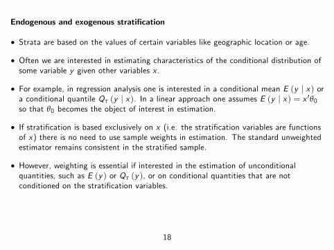
Endogenous and exogenous stratification
• Strata are based on the values of certain variables like geographic location or age.
• Often we are interested in estimating characteristics of the conditional distribution ofsome variable y given other variables x .
• For example, in regression analysis one is interested in a conditional mean E (y | x) ora conditional quantile Qτ (y | x). In a linear approach one assumes E (y | x) = x ′θ0so that θ0 becomes the object of interest in estimation.
• If stratification is based exclusively on x (i.e. the stratification variables are functionsof x) there is no need to use sample weights in estimation. The standard unweightedestimator remains consistent in the stratified sample.
• However, weighting is essential if interested in the estimation of unconditionalquantities, such as E (y ) or Qτ (y ), or on conditional quantities that are notconditioned on the stratification variables.
18

Endogenous and exogenous stratification (continued)
• More generally, in a GMM framework the condition for ignorable stratification is thatthe moment equation Eψ (W , θ0) = 0 holds in each strata:
E [ψ (W , θ0) | s ] = 0. (2)
• The intuition is that if (2) holds, E [ψ (W , θ0) | s ] ≈ 0 for all s , so we not only expect
S
∑s=1
E [ψ (W , θ0) | s ] qs =1N
N
∑i=1
ωs(i )ψ (wi , θ0) ≈ 0
but alsoS
∑s=1
E [ψ (W , θ0) | s ] hs =1N
N
∑i=1
ψ (wi , θ0) ≈ 0
19
Endogenous and exogenous stratification (continued)
Linear projections and exogenous stratification
• If a linear regression parameter θ0 only denotes a linear projection approximation to anonlinear conditional expectation E (y | x), weighting is required even if s = s (x).
• The problem is that if E [x (y − x ′θ0)] = E (xu) = 0 holds but E (y | x) 6= x ′θ0, uand x will not be uncorrelated within strata:
E (xu | s) = E [xE (u | x , s) | s ] = E [xE (u | x) | s ] 6= 0
• Intuitively, a linear regression best approximates E (y | x) at high density values of x .Since stratification changes the density of x it will also change the approximatinglinear projection.
• The same is true in an instrumental-variable model:
E[z(y − x ′θ0
)]= E (zu) = 0
if the conditional mean restriction E (u | z) = 0 does not hold. In this situationweighting will be required even if the stratification variables depend exclusively on z(more later).
20
Endogenous and exogenous stratification (continued)
• The context of the endogenous/exogenous stratification terminology is aneconometric model of y and x , which only specifies the conditional distribution of y(endogenous) given x (exogenous).
• Since the distribution of x is left unrestricted and plays no part in the estimation
f (w ) = f (y | x , θ) g (x) ,
stratification can be ignored if only modifies the form of g (x).
• In contrast, in endogenous or non-ignorable stratification, the strata are defined interms of y (and possibly other variables).
21

Population heterogeneity vs sample design• One interpretation of the weighted sample mean is that different means in each strataare first calculated and then combined into an average weighted by populationfrequencies. We wish to discuss the merits of this way of thinking in a regression case.
• Suppose that θs is a regression coeffi cient in stratum s (or some other characteristic ofthe distribution in stratum s), which varies across strata, and the object of interest is
θ =S
∑s=1
θsqs
• In general, the weighted regression estimator will not be a consistent estimator of θ.
• This is sometimes held as an argument against weighted regression: when θs arehomogeneous, unweighted regression (OLS) is more effi cient and when they are not,both weighted and unweighted estimators are inconsistent for θ (Deaton 1997).
• Where is the catch? The key is whether the substantive interest is in θ (an average ofeffects across strata) or on some quantity defined for the overall population.
• In general, the parameter θ will be of interest when variability in the θs capturesmeaningful population heterogeneity in individual responses.
• If we are using a regression as a device to summarize characteristics of the population,then θ is not the parameter of interest but rather the population-wide regressioncoeffi cient, which is precisely the object that weighted regression tries to approximate.
22
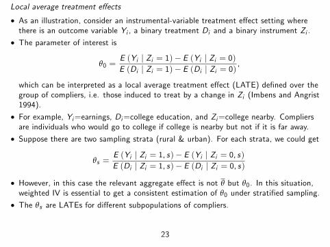
Local average treatment effects
• As an illustration, consider an instrumental-variable treatment effect setting wherethere is an outcome variable Yi , a binary treatment Di and a binary instrument Zi .
• The parameter of interest is
θ0 =E (Yi | Zi = 1)− E (Yi | Zi = 0)E (Di | Zi = 1)− E (Di | Zi = 0)
,
which can be interpreted as a local average treatment effect (LATE) defined over thegroup of compliers, i.e. those induced to treat by a change in Zi (Imbens and Angrist1994).
• For example, Yi=earnings, Di=college education, and Zi=college nearby. Compliersare individuals who would go to college if college is nearby but not if it is far away.
• Suppose there are two sampling strata (rural & urban). For each strata, we could get
θs =E (Yi | Zi = 1, s)− E (Yi | Zi = 0, s)E (Di | Zi = 1, s)− E (Di | Zi = 0, s)
• However, in this case the relevant aggregate effect is not θ but θ0. In this situation,weighted IV is essential to get a consistent estimation of θ0 under stratified sampling.
• The θs are LATEs for different subpopulations of compliers.
23
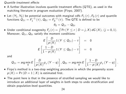
Quantile treatment effects• A further illustration involves quantile treatment effects (QTE), as used in thematching literature in program evaluation (Firpo, 2007).
• Let (Y1,Y0) be potential outcomes with marginal cdfs F1 (r ) ,F0 (r ) and quantilefunctions Q1τ = F−11 (τ) ,Q0τ = F−10 (τ). The QTE is defined to be
θ0 = Q1τ −Q0τ
• Under conditional exogeneity Fj (r ) =∫Pr (Y ≤ r | D = j ,X ) dG (X ), (j = 0, 1).
Moreover, Q1τ,Q0τ satisfy the moment conditions:
E[D
p (X )1 (Y ≤ Q1τ)− τ
]= 0
E[1−D
1− p (X )1 (Y ≤ Q0τ)− τ
]= 0
and
Q1τ = arg minqE[D
p (X )ρτ (Y − q)
],Q0τ = arg minq
E[1−D
1− p (X ) ρτ (Y − q)].
• Firpo’s method is a two-step weighting procedure in which the propensity scorep (X ) = Pr (D = 1 | X ) is estimated first.
• The point here is that in the presence of stratified sampling we would like tointroduce an additional layer of weights in both steps to undo stratification andobtain population-level quantities.
24

Choice-based sampling
• Choice-based sampling is a simple case of endogenous stratification in which y isdiscrete and its values define the strata.
• This is the context of the first econometric work on endogenous stratification.• Manski and Lerman (1977) proposed an estimator for data on individual choices oftransportation mode (travel to work by bus or by car), using choice based sampling.
• Their weighted estimator is consistent and computationally straightforward, butineffi cient in an ML context such as this one.
• The problem is that while endogenous stratification is used to oversample the rarealternative, the Manski-Lerman estimator dilutes the information by assigning lowweights to the extra observations (Coslett 1993).
• A GMM effi cient estimator is proposed in Imbens (1992).
• In an exogenously stratified sample, the informative part of the likelihood is thedensity of y conditioned on x . In contrast, in a choice-based sample, it is the densityof x conditioned on y , which is connected to the original model by Bayes’rule.
25
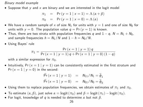
Binary model example• Suppose that y and x are binary and we are interested in the logit model
π1 = Pr (y = 1 | x = 1) = Λ (α+ β)
π0 = Pr (y = 1 | x = 0) = Λ (α)
• We have a random sample of x of size N1 for units with y = 1 and one of size N0 forunits with y = 0. The population value q = Pr (y = 1) is known.
• Thus, there are two strata with population frequencies q and 1− q, N = N1 +N0,and sample frequencies h = N1/N and 1− h = N0/N .
• Using Bayes’rule
π1 =Pr (x = 1 | y = 1) q
Pr (x = 1 | y = 1) q + Pr (x = 1 | y = 0) (1− q)with a similar expression for π0.
• Intuitively, Pr (x = 1 | y = 1) can be consistently estimated in the first stratum andPr (x = 1 | y = 0) in the second:
Pr (x = 1 | y = 1) = N11/N1 = φ1
Pr (x = 1 | y = 0) = N01/N0 = φ0
• Using them to replace population frequencies, we obtain estimates of π1 and π0.
• To estimate (α, β), just solve α = logit (π0) and β = logit (π1)− logit (π0).• For logit, knowledge of q is needed to determine α but not β.
26
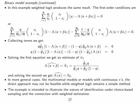
Binary model example (continued)• In this example weighted logit produces the same result. The first-order conditions are
N
∑i=1
qihi
(xi
1− xi
)[yi −Λ (α+ βxi )] = 0
orN1
∑y=1
qN1/N
(xi
1− xi
)[1−Λ (α+ βxi )]−
N0
∑y=0
1− qN0/N
(xi
1− xi
)Λ (α+ βxi ) = 0.
• Collecting terms we get:
qφ1 [1−Λ (α+ β)]− (1− q) φ0Λ (α+ β) = 0
q(1− φ1
)[1−Λ (α)]− (1− q)
(1− φ0
)Λ (α) = 0
• Solving the first equation we get an estimate of π1
Λ (α+ β) = π1 =φ1q
φ1q + φ0 (1− q)
and solving the second we get Λ (α) = π0.• In more general cases, like multinomial models or models with continuous x’s, thedirect approach may not be feasible while weighted logit remains a simple method.
• The example is intended to illustrate the nature of identification under choice-basedsampling and the connection with weighted estimation.
27

Discrete choice from data on participants
• Bover and Arellano (2002) studied the determinants of migration using choice-basedCensus data on residential variations (RV) that only had characteristics of migrants.
• The diffi culty in this case is that Pr (x = 1 | y = 0) is not identified, so that themodel parameters are not identified without further information.
• The extra information is a complementary sample from labor force surveys (LFS),which contains characteristics of migrants and non-migrants but no migrationvariables. From these data the marginal distribution of x can be estimated.
• The goal is to estimate multinomial logit probabilities of migrating to small, mediumand large towns, relying on Bayes’rule:
Pr (y = j | x) = f (x | y = j)Pr (y = j)f (x)
(j = 1, 2, 3)
• The RV data is informative about f (x | y = j) and the LFS data about f (x).
• Given RV data, LFS data are indirectly informative on nonmigrant characteristicsf (x | y = 0). Information on pj = Pr (y = j) comes from aggregate census.
28
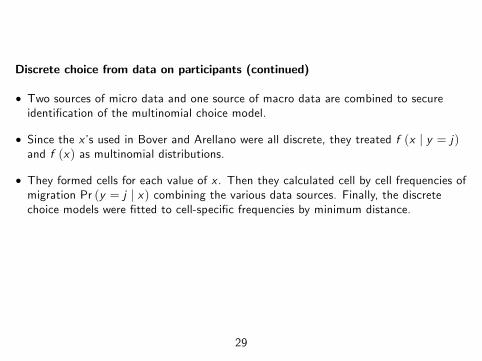
Discrete choice from data on participants (continued)
• Two sources of micro data and one source of macro data are combined to secureidentification of the multinomial choice model.
• Since the x’s used in Bover and Arellano were all discrete, they treated f (x | y = j)and f (x) as multinomial distributions.
• They formed cells for each value of x . Then they calculated cell by cell frequencies ofmigration Pr (y = j | x) combining the various data sources. Finally, the discretechoice models were fitted to cell-specific frequencies by minimum distance.
29

Continuous regressors• If x’s are continuous the previous method does not work. Here we consider a GMMalternative that works with continuous regressors. The multinomial logit model is
Pr (y = j | x) = Gj (x , θ) =ex′θj
1+ ex ′θ1 + ex ′θ2 + ex ′θ3
• Since we haveGj (x , θ) f (x) = pj f (x | y = j) ,
the following holds for any function h (x):∫h (x)Gj (x , θ) f (x) dx = pj
∫h (x) f (x | y = j) dx
• Setting h (x) = x , we have
E[xGj (x , θ)
]= pjE [x | y = j ] .
• Let the LFS data be {xk}Mk=1 and the RV data {yi , xi}Ni=1. Estimation of θ is based
on the two-sample moment conditions
1M
M
∑k=1
xkGj (xk , θ) = pj1Nj
N
∑i=1
xi1 (yi = j) (j = 1, 2, 3)
where Nj = ∑Ni=1 1 (yi = j).
30

Continuous regressors (continued)
• To see what is going on, consider the simplified situation where the model is binary(y = 1 if mover, y = 0 if stayer) and we are using a linear probability model. Theprevious moment equation boils down to
1M
M
∑k=1
xk x′k θ = p
1N
N
∑i=1
xi
• The estimator is just the following two-sample least squares method
θ = p
(1M
M
∑k=1
xk x′k
)−11N
N
∑i=1
xi
or
θ = p[ELFS
(xx ′)]−1
ERV [x | y = 1] .
31

Part 2: Cluster standard errors
32
Cluster standard errors
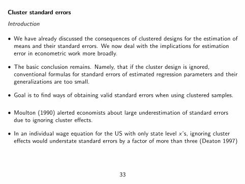
Introduction
• We have already discussed the consequences of clustered designs for the estimation ofmeans and their standard errors. We now deal with the implications for estimationerror in econometric work more broadly.
• The basic conclusion remains. Namely, that if the cluster design is ignored,conventional formulas for standard errors of estimated regression parameters and theirgeneralizations are too small.
• Goal is to find ways of obtaining valid standard errors when using clustered samples.
• Moulton (1990) alerted economists about large underestimation of standard errorsdue to ignoring cluster effects.
• In an individual wage equation for the US with only state level x’s, ignoring clustereffects would understate standard errors by a factor of more than three (Deaton 1997)
33
Remarks
• There is a close parallel between the econometrics of clustered samples and “large N ,small T”panel data (Arellano, 2003). However, in the context of clusters,unbalanced designs are the norm (varying number of units per cluster).
• For example, in a household-level panel data set, the household plays the role of acluster and time plays the role of the individual units.
• There may be also cluster samples of panel data. In those situations there are twopotential sources of correlation across observations: across time within the sameindividual and across individuals within the same cluster (see Wooldridge 2010).
• In the econometrics of clustered samples there is also an effi ciency issue, although lessprominent in applied work. The point is that because the error terms in theregressions are correlated across observations, OLS is not effi cient.
34
Cluster fixed-effects vs cluster-robust standard errors
• Sometimes within-cluster dependence is specified as an additive cluster effect in theerror of a model. In this case there is constant within-cluster correlation among errors.
• If cluster effects are correlated with regressors, within-cluster LS (cluster “fixedeffects”) is consistent but OLS in levels is not.
• If cluster effects are uncorrelated with regressors, OLS in levels is consistent butstandard errors need to be adjusted.
• Assuming constant within-cluster dependence, one can use formulas for standarderrors that are more restrictive than the fully robust formulas discussed below, butmay have better sampling properties when the number of clusters is small.
• Sometimes cluster fixed-effects are used for consistency together with cluster-robuststandard errors for correcting any remaining non-constant within-cluster correlation.
35

General set up• Let θ be a parameter identified from the moment condition
Eψ (w , θ) = 0
such that dim (θ) = dim (ψ). Consider a sample W = {w1, ...,wN } and a consistentestimator θ that solves the sample moment conditions.
• ψ (w , θ) are GMM orthogonality conditions or first-order conditions in M-estimation.
• Assume that conditions for the large-sample linear representation of the scaledestimation error and asymptotic normality hold:
√N(
θ − θ)≈ −D−10
1√N
N
∑i=1
ψ (wi , θ)d→ N
(0,D−10 V0D
−1′0
)where D0 = ∂Eψ (w , θ) /∂c ′ are partial derivatives and V0 is the limiting variance:
V0 = limN→∞
Var
(1√N
N
∑i=1
ψ (wi , θ)
)• To get standard errors of θ we need estimates of D0 and V0.
• A natural estimate of D0 is to use numerical derivatives D evaluated at θ.
• As for V0 the situation is different under independent or cluster sampling.
36
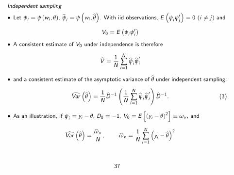
Independent sampling
• Let ψi = ψ (wi , θ), ψi = ψ(wi , θ
). With iid observations, E
(ψiψ
′j
)= 0 (i 6= j) and
V0 = E(ψiψ
′i
)• A consistent estimate of V0 under independence is therefore
V =1N
N
∑i=1
ψi ψ′i
• and a consistent estimate of the asymptotic variance of θ under independent sampling:
Var(
θ)=1ND−1
(1N
N
∑i=1
ψi ψ′i
)D−1. (3)
• As an illustration, if ψi = yi − θ, D0 = −1, V0 = E[(yi − θ)2
]≡ ωv , and
Var(
θ)=
ωvN, ωv =
1N
N
∑i=1
(yi − θ
)2
37

Cluster sampling
• The sample consists of H groups (or clusters) of Mh observations each(N = M1 + ...+MH ), such that observations are independent across groups butdependent within groups, H → ∞ and Mh is fixed for all h.
• For convenience we order observations by groups and use the double-index notationwhm so that W = {w11, ...,w1M1 | ... | wH1, ...,wHMH }.
• Under cluster sampling, letting ψh = ∑Mhm=1 ψhm and ψh = ∑Mh
m=1 ψhm we have
V0 = limN→∞
Var
(1√N
H
∑h=1
ψh
)= limN→∞
1N
H
∑h=1
E(
ψhψ′h
),
so that E(
ψiψ′j
)= 0 only if i and j belong to different clusters, or
E(ψhmψ′h′m ′
)= 0 for h 6= h′. Thus, a consistent estimate of V0 is
V =1N
H
∑h=1
ψh ψ′h .
• The estimated asymptotic variance of θ allowing within-cluster correlation is
Var(
θ)=1ND−1
(1N
H
∑h=1
ψh ψ′h
)D−1. (4)
• Note that (4) is of order 1/H whereas (3) is of order 1/N .38
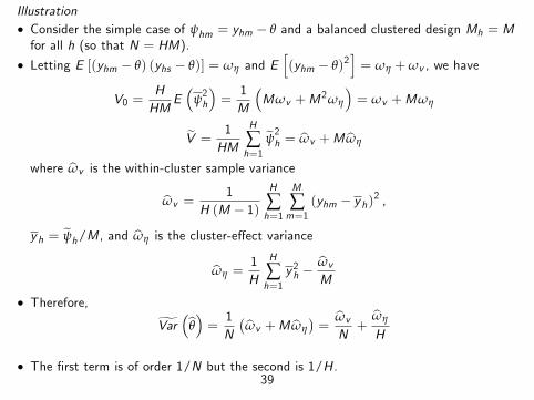
Illustration• Consider the simple case of ψhm = yhm − θ and a balanced clustered design Mh = Mfor all h (so that N = HM).
• Letting E [(yhm − θ) (yhs − θ)] = ωη and E[(yhm − θ)2
]= ωη +ωv , we have
V0 =HHM
E(
ψ2h
)=1M
(Mωv +M2ωη
)= ωv +Mωη
V =1HM
H
∑h=1
ψ2h = ωv +M ωη
where ωv is the within-cluster sample variance
ωv =1
H (M − 1)H
∑h=1
M
∑m=1
(yhm − y h)2 ,
y h = ψh/M , and ωη is the cluster-effect variance
ωη =1H
H
∑h=1
y 2h −ωvM
• Therefore,
Var(
θ)=1N
(ωv +M ωη
)=
ωvN+
ωη
H
• The first term is of order 1/N but the second is 1/H .39

Examples
Panel data model
• A panel data example is
ψ (whm , θ) = xhm(yhm − x ′hmθ
)where h denotes units and m time periods. If the variables are in deviations frommeans, θ is the within-group estimator.
• In this case Dhm = −xhmx ′hm and ψh = ∑Mhm=1 xhm uhm where uhm are within-group
residuals.
• The result is the (large H , fixed Mh) formula for within-group standard errors that arerobust to heteroskedasticity and serial correlation of arbitrary form in Arellano (1987):
Var(
θ)=
(H
∑h=1
Mh
∑m=1
xhmx′hm
)−1 H
∑h=1
Mh
∑m=1
Mh
∑s=1
uhm uhsxhmx′hs
(H
∑h=1
Mh
∑m=1
xhmx′hm
)−1
40
Examples (continued)
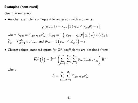
Quantile regression
• Another example is a τ-quantile regression with moments
ψ (whm , θ) = xhm[1(yhm ≤ x ′hmθ
)− τ
]where Dhm = ωhmxhmx ′hm , ωhm = 1
(∣∣∣yhm − x ′hm θ∣∣∣ ≤ ξN
)/ (2ξN ),
ψh = ∑Mhm=1 xhm uhm and uhm = 1
(yhm ≤ x ′hm θ
)− τ.
• Cluster-robust standard errors for QR coeffi cients are obtained from:
Var(
θ)= B−1
(H
∑h=1
Mh
∑m=1
Mh
∑s=1
uhm uhsxhmx′hs
)B−1
where
B =H
∑h=1
Mh
∑m=1
ωhmxhmx′hm
41
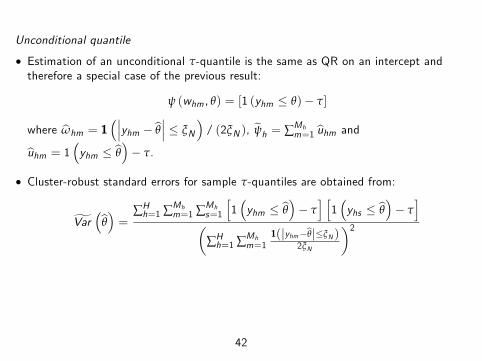
Unconditional quantile
• Estimation of an unconditional τ-quantile is the same as QR on an intercept andtherefore a special case of the previous result:
ψ (whm , θ) = [1 (yhm ≤ θ)− τ]
where ωhm = 1(∣∣∣yhm − θ
∣∣∣ ≤ ξN
)/ (2ξN ), ψh = ∑Mh
m=1 uhm and
uhm = 1(yhm ≤ θ
)− τ.
• Cluster-robust standard errors for sample τ-quantiles are obtained from:
Var(
θ)=
∑Hh=1 ∑Mhm=1 ∑Mh
s=1
[1(yhm ≤ θ
)− τ
] [1(yhs ≤ θ
)− τ
](
∑Hh=1 ∑Mhm=1
1(|yhm−θ|≤ξN )2ξN
)2
42

Part 3: Bootstrap methods
43
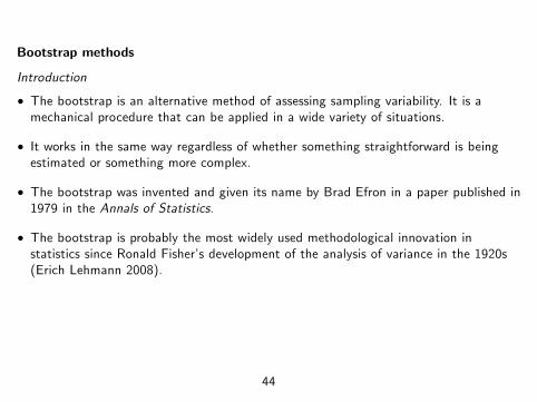
Bootstrap methods
Introduction
• The bootstrap is an alternative method of assessing sampling variability. It is amechanical procedure that can be applied in a wide variety of situations.
• It works in the same way regardless of whether something straightforward is beingestimated or something more complex.
• The bootstrap was invented and given its name by Brad Efron in a paper published in1979 in the Annals of Statistics.
• The bootstrap is probably the most widely used methodological innovation instatistics since Ronald Fisher’s development of the analysis of variance in the 1920s(Erich Lehmann 2008).
44
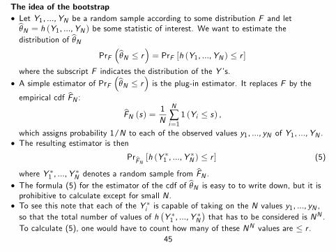
The idea of the bootstrap• Let Y1, ...,YN be a random sample according to some distribution F and let
θN = h (Y1, ...,YN ) be some statistic of interest. We want to estimate thedistribution of θN
PrF(
θN ≤ r)= PrF [h (Y1, ...,YN ) ≤ r ]
where the subscript F indicates the distribution of the Y ’s.• A simple estimator of PrF
(θN ≤ r
)is the plug-in estimator. It replaces F by the
empirical cdf FN :
FN (s) =1N
N
∑i=1
1 (Yi ≤ s) ,
which assigns probability 1/N to each of the observed values y1, ..., yN of Y1, ...,YN .• The resulting estimator is then
PrFN [h (Y∗1 , ...,Y
∗N ) ≤ r ] (5)
where Y ∗1 , ...,Y∗N denotes a random sample from FN .
• The formula (5) for the estimator of the cdf of θN is easy to to write down, but it isprohibitive to calculate except for small N .
• To see this note that each of the Y ∗i is capable of taking on the N values y1, ..., yN ,so that the total number of values of h
(Y ∗1 , ...,Y
∗N
)that has to be considered is NN .
To calculate (5), one would have to count how many of these NN values are ≤ r .45
The idea of the bootstrap (continued)
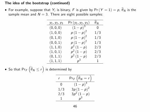
• For example, suppose that Yi is binary, F is given by Pr (Y = 1) = p, θN is thesample mean and N = 3. There are eight possible samples:
y1, y2, y3 Pr (y1, y2, y3) θN(0, 0, 0) (1− p)3 0(1, 0, 0) p (1− p)2 1/3(0, 1, 0) p (1− p)2 1/3(0, 0, 1) p (1− p)2 1/3(1, 1, 0) p2 (1− p) 2/3(1, 0, 1) p2 (1− p) 2/3(0, 1, 1) p2 (1− p) 2/3(1, 1, 1) p3 1
• So that PrF(
θN ≤ r)is determined by
r PrF(
θN = r)
0 (1− p)31/3 3p (1− p)22/3 3p2 (1− p)1 p3
46
The idea of the bootstrap (continued)
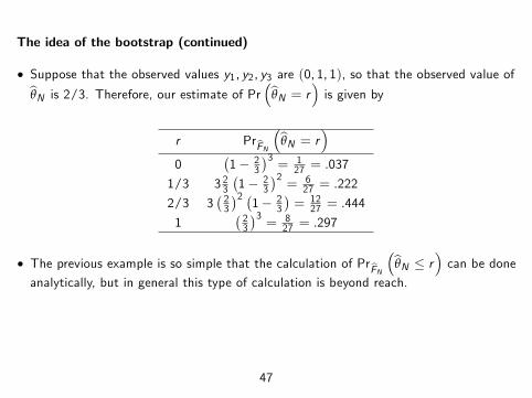
• Suppose that the observed values y1, y2, y3 are (0, 1, 1), so that the observed value ofθN is 2/3. Therefore, our estimate of Pr
(θN = r
)is given by
r PrFN
(θN = r
)0
(1− 2
3
)3= 1
27 = .037
1/3 3 23(1− 2
3
)2= 6
27 = .222
2/3 3( 23
)2 (1− 2
3
)= 12
27 = .444
1( 23
)3= 8
27 = .297
• The previous example is so simple that the calculation of PrFN
(θN ≤ r
)can be done
analytically, but in general this type of calculation is beyond reach.
47
The idea of the bootstrap (continued)
Estimation by simulation
• A standard device for (approximately) evaluating probabilities that are too diffi cult tocalculate exactly is simulation.
• To calculate the probability of an event, one generates a sample from the underlyingdistribution and notes the frequency with which the event occurs in the generatedsample.
• If the sample is suffi ciently large, this frequency will provide an approximation to theoriginal probability with a negligible error.
• Such approximation to the probability (5) constitutes the second step of thebootstrap method.
• A number M of samples Y ∗1 , ...,Y∗N (the “bootstrap” samples) are drawn from FN ,
and the frequency with which
h (Y ∗1 , ...,Y∗N ) ≤ r
provides the desired approximation to the estimator (5) (Lehmann 2008).
48
Numerical illustration
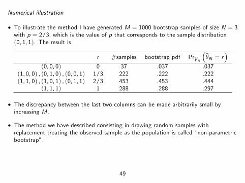
• To illustrate the method I have generated M = 1000 bootstrap samples of size N = 3with p = 2/3, which is the value of p that corresponds to the sample distribution(0, 1, 1). The result is
r #samples bootstrap pdf PrFN
(θN = r
)(0, 0, 0) 0 37 .037 .037
(1, 0, 0) , (0, 1, 0) , (0, 0, 1) 1/3 222 .222 .222(1, 1, 0) , (1, 0, 1) , (0, 1, 1) 2/3 453 .453 .444
(1, 1, 1) 1 288 .288 .297
• The discrepancy between the last two columns can be made arbitrarily small byincreasing M .
• The method we have described consisting in drawing random samples withreplacement treating the observed sample as the population is called “non-parametricbootstrap”.
49
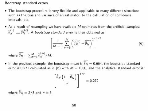
Bootstrap standard errors
• The bootstrap procedure is very flexible and applicable to many different situationssuch as the bias and variance of an estimator, to the calculation of confidenceintervals, etc.
• As a result of resampling we have available M estimates from the artificial samples:
θ(1)N , ..., θ
(M )N . A bootstrap standard error is then obtained as[
1M − 1
M
∑m=1
(θ(m)N − θN
)2]1/2
(6)
where θN = ∑Mm=1 θ(m)N /M .
• In the previous example, the bootstrap mean is θN = 0.664, the bootstrap standarderror is 0.271 calculated as in (6) with M = 1000, and the analytical standard error is θN
(1− θN
)n
1/2
= 0.272
where θN = 2/3 and n = 3.
50

Asymptotic properties of bootstrap methods
• Using the bootstrap standard error to construct test statistics cannot be shown toimprove on the approximation provided by the usual asymptotic theory, but the goodnews is that under general regularity conditions it does have the same asymptoticjustification as conventional asymptotic procedures.
• This is good news because bootstrap standard errors are often much easier to obtainthan analytical standard errors.
Refinements for large-sample pivotal statistics• Even better news is the fact that in many cases the bootstrap does improve theapproximation of the distribution of test statistics, in the sense that the bootstrap canprovide an asymptotic refinement compared with the usual asymptotic theory.
• The key aspect for achieving such refinements (consisting in having an asymptoticapproximation with errors of a smaller order of magnitude in powers of the samplesize) is that the statistic being bootstraped is asymptotically pivotal.
• An asymptotically pivotal statistic is one whose limiting distribution does not dependon unknown parameters (like standard normal or chi-square distributions).
• This is the case with t-ratios and Wald test statistics, for example.• Note that for a t-ratio to be asymptotically pivotal in a regression with heteros-kedasticity, the robust White form of the t-ratio needs to be used.
51

Asymptotic properties of bootstrap methods (continued)
• The upshot of the previous discussion is that the replication of the quantity of interest(mean, median, etc.) is not always the best way to use the bootstrap if improvementson asymptotic approximations are sought.
• In particular, when we wish to calculate a confidence interval, it is better not tobootstrap the estimate itself but rather to bootstrap the distribution of the t-value.
• This is feasible when we have a large sample estimate of the standard error, but one isskeptical about the accuracy of the normal probability approximation.
• Such procedure will provide more accurate estimates of confidence intervals thaneither the simple bootstrap or the asymptotic standard errors.
• However, often we are interested in bootstrap methods because an analytic standarderror is not available or is hard to calculate.
• In those cases the motivation for the bootstrap is not necessarily improving on theasymptotic approximation but rather obtaining a simpler approximation with the samejustification as the conventional asymptotic approximation.
52
Bootstrapping stratified clustered samples
• The bootstrap can be applied to a stratified clustered sample.
• All we have to do is to treat the strata separately, and resample, not the basicunderlying units (the households) but rather the primary sample units (the clusters).
53

Using replicate weights
• Taking stratification and clustering sampling features into account, either analyticallyor by bootstrap, requires the availability of stratum and cluster indicators.
• Generally, Statistical Offi ces or survey providers do not make them available forconfidentiality reasons.
• To enable the estimation of the sampling distribution of estimators and test statisticswithout disclosing stratum or cluster information, an alternative is to provide replicateweights.
• For example, the EFF provides 999 replicate weights. Specifically the EFF providesreplicate cross-section weights, replicate longitudinal weights, and multiplicity factors(Bover, 2004).
• Multiplicity factors indicate the number of times a given household appears in aparticular bootstrap sample.
• The provision of replicate weights is an important development because it facilitatesthe use of replication methods, which are simple and of general applicability, togetherwith allowing for confidentiality safe ward.
54

References
Arellano, M. (1987): “Computing Robust Standard Errors for Within-GroupEstimators”, Oxford Bulletin of Economics and Statistics, 49, 431-434.
Arellano, M. (2003): Panel Data Econometrics, Oxford University Press.
Bover, O. and M. Arellano (2002): “Learning About Migration Decisions From theMigrants,” Journal of Population Economics, 15, 357-380.
Bover, O. (2004), “The Spanish Survey of Household Finances (EFF): Descriptionand Methods of the 2002 Wave”, Banco de España Occasional Paper 0409.
Deaton, A. (1997): The Analysis of Household Surveys: A MicroeconometricApproach to Development Policy, Johns Hopkins Press.
Cameron, C. and P. Trivedi (2005): Microeconometrics, Cambridge UniversityPress.
Coslett, S. R. (1993): “Estimation from Endogenously Stratified Samples,” in G.S.Maddala, C.R. Rao, and H.D. Vinod (eds.): Handbook of Statistics, Vol. 11, NorthHolland.
Efron, B. (1979): “Bootstrap Methods: Another Look at the Jackknife,”Annals ofStatistics, 7, 1—26.
Firpo, S. (2007): “Effi cient Semiparametric Estimation of Quantile TreatmentEffects,”Econometrica, 75, 259—276.
55

References (continued)
Imbens, G. (1992): “An Effi cient Method of Moments Estimator for DiscreteChoice Models with Choice-Based Sampling,”Econometrica, 60, 1187—1214.
Imbens, G. W. and J. Angrist (1994): “Identification and Estimation of LocalAverage Treatment Effects”, Econometrica, 62, 467-475.
Imbens, G. and T. Lancaster (1996): “Effi cient Estimation and StratifiedSampling,” Journal of Econometrics, 74, 289—318.
Levy, P. S. and S. Lemeshow (1991): Sampling of Populations: Methods andApplications, 2nd edition, Wiley.
Manski, C. F. and S. R. Lerman (1977): “The Estimation of Choice Probabilitiesfrom Choice Based Samples,”Econometrica, 45, 1977-1988.
Moulton, B. R. (1990): “An Illustration of a Pitfall in Estimating the Effects ofAggregate Variables on Micro Units,”Review of Economics and Statistics, 72,334-338
Ullah, A. and R. V. Breunig (1998): “Econometric Analysis in Complex Surveys,”in D. Giles and A. Ullah (eds.): Handbook of Applied Economic Statistics, MarcelDekker.
Wooldridge, J. M. (2010): Econometric Analysis of Cross Section and Panel Data,2nd edition, MIT Press.
56