Embed Size (px)
Citation preview
Economic Depreciation in the Property Value:
Cross-Sectional Variations and Their Implications on Investments∗
Jiro Yoshida†
December 14, 2017
Abstract
This study compares the rate of property value depreciation between different property types,
locations, and countries by using commercial and residential data for the U.S. and Japan. The
property-level depreciation rate is larger if a property is commercial, newer, denser, located in
a smaller city, more distant from the central business district, and in Japan. A larger depreci-
ation rate directly decreases appreciation returns and increases the equilibrium income returns
(i.e., cap rates). The depreciation rate for the structure component also varies significantly by
property type and country; approximately 7% for residential properties and 10% for commer-
cial properties in Japan in contrast with 1% for residential structures in the U.S. This study
also demonstrates the difference in the estimation methods and the importance of correcting
survivorship biases. These results serve as important inputs for the analysis of real estate
investment, consumer choice of housing, sustainability, and macro economy.
JEL Classification: R32; D24; E23
Keywords: capital consumption, housing, commercial real estate, hedonic analysis, survivorshipbias, demolition, Japan, USA
∗I thank Lorraine Spock, Real Capital Analytics, Japanese Ministry of Land, Infrastructure, Transport, andTourism for providing data. I gratefully acknowledge research assistance from Conor Doyle and Sergio Garate. Thispaper is supported by the Real Estate Research Institute.†Smeal College of Business, The Pennsylvania State University, 368 Business Building, University Park, PA 16802,

I. Introduction
The economic depreciation of real estate is important in a wide range of economic analysis
and decision making. First, in real estate investments, a large depreciation rate implies small
appreciation returns and large income returns. Thus, the component returns can significantly vary
simply due to variations in depreciation rates by country, city, urban location, building age, and
property type. Because investors choose portfolios by taking into account the proportions of income
and appreciation returns for the purpose of liquidity management, investor asset allocations are
influenced by the cross-sectional variation in depreciation rate.
Second, in macroeconomics, structure depreciation rates are a key parameter in models of eco-
nomic growth and fluctuations (e.g., Greenwood and Hercowitz, 1991; Davis and Heathcote, 2005;
Davis and Nieuwerburgh, 2015). For example, depreciation rates affect the equilibrium level capital,
consumption, saving, and productivity.1 Depreciation rates are also a key input to macroeconomic
statistics such as gross domestic product and inflation rates, which influence monetary and other
macroeconomic policies (e.g., Ambrose, Coulson, and Yoshida, 2015).
Third, in housing economics, the depreciation rate of housing affects consumer choice, welfare,
and the environmental sustainability. For example, a large depreciation rate increases the user cost
and rental cost of housing. Since housing services are complementary to other goods (Davidoff
and Yoshida, 2013), large depreciation makes households to spend a larger share of income on
housing. Residential properties that depreciate more slowly than standard properties are traded
at a premium (Yoshida and Sugiura, 2015). Larger depreciation also has an adverse environmental
consequence because more frequent demolitions of structures increase CO2 emissions.
This study has three objectives. The first objective is to demonstrate significant cross-sectional
variation in the property-level depreciation rate. Because the property-level depreciation rate is
directly proportional to the structure value share, the depreciation rate and the structure value
share will exhibit similar variation. The urban economic theory predicts that the structure value
share is affected by the city size, the location within a city, the building age, the density of a
property, and other factors (e.g., Alonso, 1964; Muth, 1969; Mills, 1967; Fujita, 1989; Duranton
1The measurement of depreciation rates is central to understanding Japan’s high saving rate (e.g., Hayashi, 1986,1989, 1991; Hayashi, Ito, and Slemrod, 1987; Dekle and Summers, 1991; Hayashi and Prescott, 2002; Imrohoroglu,Imrohoroglu, and Chen, 2006).
1
and Puga, 2015). I estimate the effect of building age on property values by using data for the U.S.
residential properties (Centre County, PA) and the Japanese residential and commercial properties.
The estimated variation is economically significant (up to 3.5% per year) and consistent with the
urban economic theory for both countries; i.e., the property depreciation rate is larger for newer and
denser properties located away from the Central Business District (CBD) in a smaller city. Since
depreciation rates have a direct impact on the proportions of income and appreciation returns, this
result provides a new insight into the variation in real estate returns.
The second objective is to estimate the structure depreciation rate. I estimate the net depre-
ciation rate, which is the rate after maintenance and capital expenditures are made.2 I use two
estimation methods. The first method is to adjust the property-level depreciation rate for the
structure value share. For example, if the property-level depreciation rate is 1% and the struc-
ture value share is 0.2, then the implied structure depreciation rate is 5% (1%/0.2) because other
components of property value do not depreciate with building age. The structure value share is
estimated by the elasticity of property value with respect to the size of structure in the hedonic
regression. The estimated share is significantly smaller in Japan (30%-40% at median ages) than in
the U.S. (50%-70%) whereas the land value share is significantly larger in Japan (60%-70%) than
in the U.S. (10%). The larger proportion of land value probably reflects the scarcity of habitable
land in Japan.3
The second method of estimating the structure depreciation rate uses the building age infor-
mation at the time of demolition. Buildings are demolished when the depreciated structure value
equals the scrap value, which is implicitly determined by the owner’s redevelopment decision. I
make an assumption about the scrap value and estimate the average annual depreciation rate over
building life. For example, if the scrap value is 10% of the original value, the average depreciation
rate is 4.6% per year for a demolished 50-year old building (− ln 0.1/50). Using the demolition data
in Japan, I estimate the frequency distribution of depreciation rates for various property types.
The mean depreciation rate is 6.2% for residential, 9.2% for industrial, 11.7% for office, 14.8% for
retail, and 17.2% for hotel property. These estimates are consistent with the estimates by the first
2The data in this study do not include maintenance expenditures. For an estimate of gross depreciation rate ofcommercial real estate value in the U.S., see Geltner and Bokhari (2015).
3The habitable area is only approximately 30% of the national land; large part is forest, mountains, and waters.Therefore, population density is 50 times larger in Japan than in the United States.
2
method.
The third objective is to develop and empirically demonstrate new methods of correcting for
survivorship biases in the estimation of structure depreciation rates. When the econometrician
estimates depreciation rates using a sample of surviving buildings, the estimated rate is too small
(Hulten and Wykoff, 1981b). Because buildings with the largest depreciation rate are demolished
first, this survivorship bias does not exist for the sample of new buildings and becomes larger for
the sample of older buildings. In contrast, when the econometrician uses a sample of demolished
buildings, the estimated rate is too large. The observed distribution of building life span is skewed
because shorter-lived buildings are more frequently demolished. The distribution is additionally
distorted by the past variation in the construction volume; e.g., the econometrician will observe a
larger number of 50-year old buildings in the demolished sample if the construction volume was
large 50 years ago. To address the former type of biases for surviving buildings, I focus on the mean
depreciation rate for relatively new buildings because the estimated rate is unbiased if no building
is demolished. I additionally show a distribution of depreciation rates that is consistent with the
observed survivorship bias. To address the latter type of estimation biases for demolished buildings,
I correct the distribution of building life spans for the oversampling of short-lived structures and
past variation in construction volume.
The proposed methods of bias correction have several advantages. First, they do not require data
on both surviving and demolished buildings unlike standard methods such as the Cox proportional
hazard rate model, the Kaplan-Meier estimator, and Heckman’s two-step procedure. Second, the
proposed methods improve the method by Hulten and Wykoff (1981b). They assume that the
depreciation rate for demolished structures is zero by treating the value of demolished structures
being zero. In contrast, I incorporate large depreciation rates for demolished buildings based on a
distributional assumption. However, the proposed methods do not address the maintenance effect,
the vintage effect, or the selection for sold properties. The current data set contains no information
on maintenance and is too short to estimate the vintage effect as Coulson and McMillen (2008)
do. This study can be extended if a richer and longer data set is available. The selection issue is
partially mitigated because this study focuses only on traded properties.
The bias-corrected rate of structure depreciation also varies widely by country and the estima-
tion method. The structure depreciation rate based on the price data is 6.4%-7.0% for residential
3
properties and 9.1%-10.2% for commercial properties in Japan whereas it is 1.5% for residential
properties in the U.S. These rates are consistent with those based on the demolition data in Japan.
The bias corrected median life span of structures in Japan is 30-35 years for residential and 20-
30 years for commercial properties. The property-type specific depreciation rate for commercial
properties in Japan is 7.8% for industrial, 9.9% for office, 14.6% for hotel, and 12.6% for retail prop-
erties. Since researchers have not reached a consensus regarding the level of aggregate structure
depreciation rates, the estimated rate serves as an important input for macroeconomic models.
The large depreciation rates in Japan could be caused by cultural, historical, and institutional
factors. For example, a lack of reliable information about building inspections can cause adverse
selection and moral hazard. In such a bad equilibrium, maintenance expenditures will be small
and depreciation rates will be large. Cultural and behavioral biases can be another cause. People’s
perceptions about building life spans were formed on the basis of traditional structures that were
vulnerable to earthquakes and fire. Although modern structures are significantly more robust to
these risks, people’s perceptions have not changed very much. Indeed, a rapid progress in building
technologies is a major factor of large depreciation. In particular, given that approximately 20% of
large earthquakes on earth occur in and around Japan (Cabinet Office of Japan, 2013), technological
progress in earthquake resistance was large in the 20th century. The earthquake resistance standard
in the national building code was repeatedly revised in 1950 (after Fukui earthquake), 1971 (after
Tokachi earthquake), 1981 (after Miyagi earthquake), and 2000 (after Hanshin-Awaji earthquake).
The proportion of structures that were directly damaged by earthquakes was not large in the
national stock of structures. However, the existing buildings became obsolete relatively quickly due
to the rapid progress in building technologies. Moreover, many existing buildings became out of
compliance after revisions to the national building code.
The extant studies use different methods and show a wide range of estimated depreciation rate.
The first method utilizes time-series or cross-sectional variations in asset prices (e.g., Hulten and
Wykoff, 1981a; Coulson and McMillen, 2008; Yoshida and Sugiura, 2015; Geltner and Bokhari,
2015). A cross-sectional hedonic regression is often used because of better data availability. The
second method combines the flow investment data and the real estate stock data, typically in
the National Accounts (e.g., Hulten and Wykoff, 1981a; Hayashi, 1991; Yoshida and Ha, 2001;
Economic and Social Research Institute, 2011). The implicit depreciation rate in the accumulation
4

equation is estimated. The third method utilizes the data on demolished buildings. Structure
depreciation rates are estimated by the building age at the time of demolition. This is more common
in engineering studies. The estimated depreciation rates for the U.S. commercial structures are large
and exhibit variations; they are 2.0% for retail, 2.5% for office, 2.7% for warehouse, and 3.6% for
factory based on asset prices (Hulten and Wykoff, 1981b) but 5.2%-7.2% based on the implicit
rate in the National Accounts published by the Buerau of Economic Analysis (Hulten and Wykoff,
1981a; Hayashi, 1991). In a recent study that uses asset prices, the rate is approximately 3% for
all commercial real estate and 3.3%-4.0% for apartments (Fisher, Smith, Stern, and Webb, 2005;
Geltner and Bokhari, 2015). The estimated rates for the U.S. residential structures fall within a
relatively narrow range; they are 1.36% (Leigh, 1980), 1.89% (Knight and Sirmans, 1996), and
1.94% (Harding, Rosenthal, and Sirmans, 2007) based on asset prices.4 Based on the National
Accounts, the rate is 1.57% between 1948 and 2001 (Davis and Heathcote, 2005). The estimated
rates for residential structures in Japan range from as low as 1%-2% (Seko, 1998) to 15% (Yoshida
and Ha, 2001). Based on the National Accounts of Japan, the depreciation rate is 8.5%-9.9% when
data between 1970 and 1989 is used (Hayashi, 1991) but the rate is 4.7% and 5.4% when newer
data are used (Economic and Social Research Institute, 2011).5 For non-residential (commercial)
structures, a few available estimates based on the National Accounts are 5.7%-7.2% (Hayashi, 1991;
Economic and Social Research Institute, 2011).
The remaining sections proceed as follows. In Section II, I present the conceptual framework
and two methods of bias correction. Section III discusses the data and summary statistics, and
Section IV outlines the empirical strategy. Sections V and VI present the empirical results. Section
VII concludes.
II. Conceptual Framework
The value Vt,u of a property of age u is determined in the real estate asset market at time t.
The property value can be decomposed into three factors: structure value, land value, and any
4However, the effect of aging on residential rents is significanlty smaller at 0.11% to 0.36% (Lane, Randolph, andBerenson, 1988).
5The depreciation rate also varies by prefecture, property type, whether a property is for rental or not, andwhether a property is a green building or not (Yoshida and Ha, 2001; Yoshida, Yamazaki, and Lee, 2009; Yamazakiand Sadayuki, 2010; Yoshida and Sugiura, 2015)
5
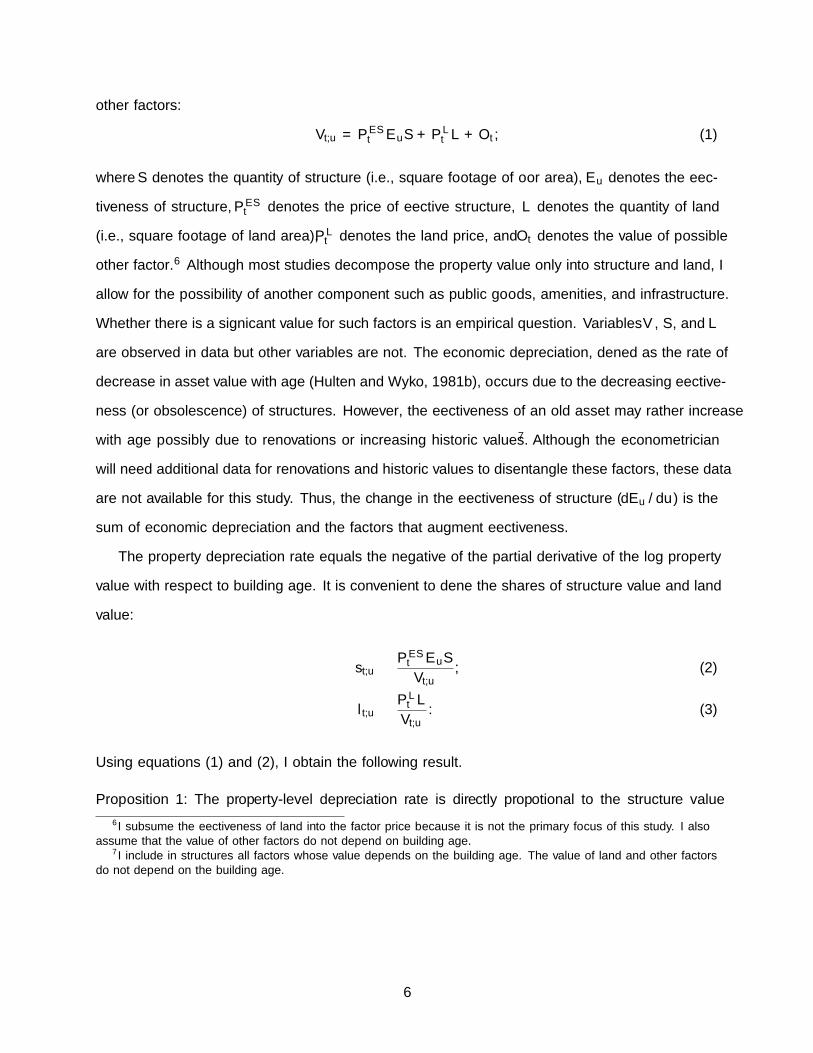
other factors:
Vt,u = PESt EuS + PLt L+Ot, (1)
where S denotes the quantity of structure (i.e., square footage of floor area), Eu denotes the effec-
tiveness of structure, PESt denotes the price of effective structure, L denotes the quantity of land
(i.e., square footage of land area), PLt denotes the land price, and Ot denotes the value of possible
other factor.6 Although most studies decompose the property value only into structure and land, I
allow for the possibility of another component such as public goods, amenities, and infrastructure.
Whether there is a significant value for such factors is an empirical question. Variables V , S, and L
are observed in data but other variables are not. The economic depreciation, defined as the rate of
decrease in asset value with age (Hulten and Wykoff, 1981b), occurs due to the decreasing effective-
ness (or obsolescence) of structures. However, the effectiveness of an old asset may rather increase
with age possibly due to renovations or increasing historic values.7 Although the econometrician
will need additional data for renovations and historic values to disentangle these factors, these data
are not available for this study. Thus, the change in the effectiveness of structure (dEu /du) is the
sum of economic depreciation and the factors that augment effectiveness.
The property depreciation rate equals the negative of the partial derivative of the log property
value with respect to building age. It is convenient to define the shares of structure value and land
value:
st,u ≡PESt EuS
Vt,u, (2)
lt,u ≡PLt L
Vt,u. (3)
Using equations (1) and (2), I obtain the following result.
Proposition 1: The property-level depreciation rate is directly propotional to the structure value
6I subsume the effectiveness of land into the factor price because it is not the primary focus of this study. I alsoassume that the value of other factors do not depend on building age.
7I include in structures all factors whose value depends on the building age. The value of land and other factorsdo not depend on the building age.
6

ratio and the structure depreciation rate: i.e.,
− ∂ lnVt,u∂u
= st,uδu, (4)
where δu ≡ −d lnEu /du denotes the instantaneous depreciation rate of structures.
Proof. Take the logarithm of both sides of equation (1). The partial derivative of lnVt,u with
respect to u is:
∂ lnVt,u∂u
=PESt S
Vt,u
dEudu
=PESt EuS
Vt,u
1
Eu
dEudu
= st,ud lnEudu
= −st,uδu.
Since the structure value share st,u is less than one, the property depreciation rate is always
smaller in absolute value than the structure depreciation rate. However, the structure value could
appreciate with age after removing the inflation effect (i.e., δu < 0) possibly due to renovations or
increasing historical values.
When the property value changes with building age, the structure value share also changes.
Proposition 2: The structure value share increases (decreases) with building age if and only if the
property value increases (decreases) with building age.
Proof. Take a partial derivative of the structure value share with respect to the building age in
equation (2).
∂st,u∂u
=PESt SdEu /du
Vt,u−(PESt EuS
) (PESt SdEu /du
)V 2t,u
=
(1− PESt EuS
Vt,u
)PESt SdEu /du
Vt,u
= (1− st,u)∂ lnVt,u∂u
.
7

Since the first term (1− st,u) is positive, I obtain: sgn (∂st,u /∂u) = sgn (d lnEu /du).
When estimating depreciation rates and the structure value share using the actual data, an
econometrician can only observe the nominal value of a property and the quantities of structure
and land. Using these observable variables, I estimate the shares of structure value and land value
by calculating the elasticity of property value with respect to the quantities of structure and land:
∂ lnVt,u∂ lnS
=∂Vt,u∂S
S
Vt,u=PESt EuS
Vt,u= st,u, (5)
∂ lnVt,u∂ lnL
=∂Vt,u∂L
L
Vt,u=PLt L
Vt,u= lt,u. (6)
I use these elasticities to estimate the structure depreciation rate δu on the basis of equation (4).
This method has an advantage over another popular method of estimating the structure value
share. For example, Yoshida, Yamazaki, and Lee (2009) and Geltner and Bokhari (2015) estimate
the land value share by taking the ratio of the value of old properties to the value of new properties,
and subtract the land value share from one. There are several implicit assumptions in this method.
First, the structure value must be approximately zero for old properties. This may not be the case
when historical values are attached to structures. Second, the structure value share must equal one
minus the land value share. This may not be the case if there is the third factor with a fixed value.
In the next three sections, I discuss how the structure value share, property-level depreciation
rates, and income returns varies by location (II.A) and how to correct for biases in estimating the
structure depreciation rate from price data (II.B) and from demolition data (II.C).
A. Cross-Sectional Variation in Property Depreciation Rates
The structure value share varies by location in the urban economic theory. In particular, the
monocentric city model of urban land use predicts that the structure value share varies by city
size (e.g., population) and urban location (e.g., distance to the CBD) for several reasons. For
example, Duranton and Puga (2015) summarize the following predictions of the basic monocentric
city model. First, for newly developed properties, land prices decline as one moves away from
the CBD. Since the unit cost of structures is by and large constant within a city, the property
value also exhibits a declining price gradient. Second, the density of construction declines as one
8
moves away from the CBD. Since the physical land ratio increases and the land price decreases
with distance, whether the land value share decreases with distance depends on these competing
effects. In spatial equilibrium, the land value share equals the ratio of the percentage decline in
the property price to the percentage decline in the land price with distance. Third, the differential
land price between the CBD and the edge of the city should be proportional to the city population
and the unit commuting cost.
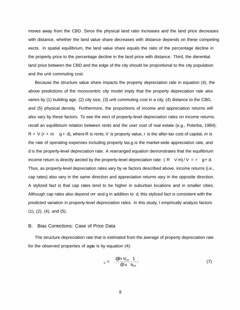
Because the structure value share impacts the property depreciation rate in equation (4), the
above predictions of the monocentric city model imply that the property depreciation rate also
varies by (1) building age, (2) city size, (3) unit commuting cost in a city, (4) distance to the CBD,
and (5) physical density. Furthermore, the proportions of income and appreciation returns will
also vary by these factors. To see the effect of property-level depreciation rates on income returns,
recall an equilibrium relation between rents and the user cost of real estate (e.g., Poterba, 1984):
R = V (r +m− g + d), where R is rents, V is property value, r is the after-tax cost of capital, m is
the rate of operating expenses including property tax, g is the market-wide appreciation rate, and
d is the property-level depreciation rate. A rearranged equation demonstrates that the equilibrium
income return is directly affected by the property-level depreciation rate: (R−V m) /V = r−g+d.
Thus, as property-level depreciation rates vary by five factors described above, income returns (i.e.,
cap rates) also vary in the same direction and appreciation returns vary in the opposite direction.
A stylized fact is that cap rates tend to be higher in suburban locations and in smaller cities.
Although cap rates also depend on r and g in addition to d, this stylized fact is consistent with the
predicted variation in property-level depreciation rates. In this study, I empirically analyze factors
(1), (2), (4), and (5).
B. Bias Corrections: Case of Price Data
The structure depreciation rate that is estimated from the average of property depreciation rate
for the observed properties of age u is by equation (4):
δ̄u = −∂ lnVt,u∂u
1
st,u. (7)
9
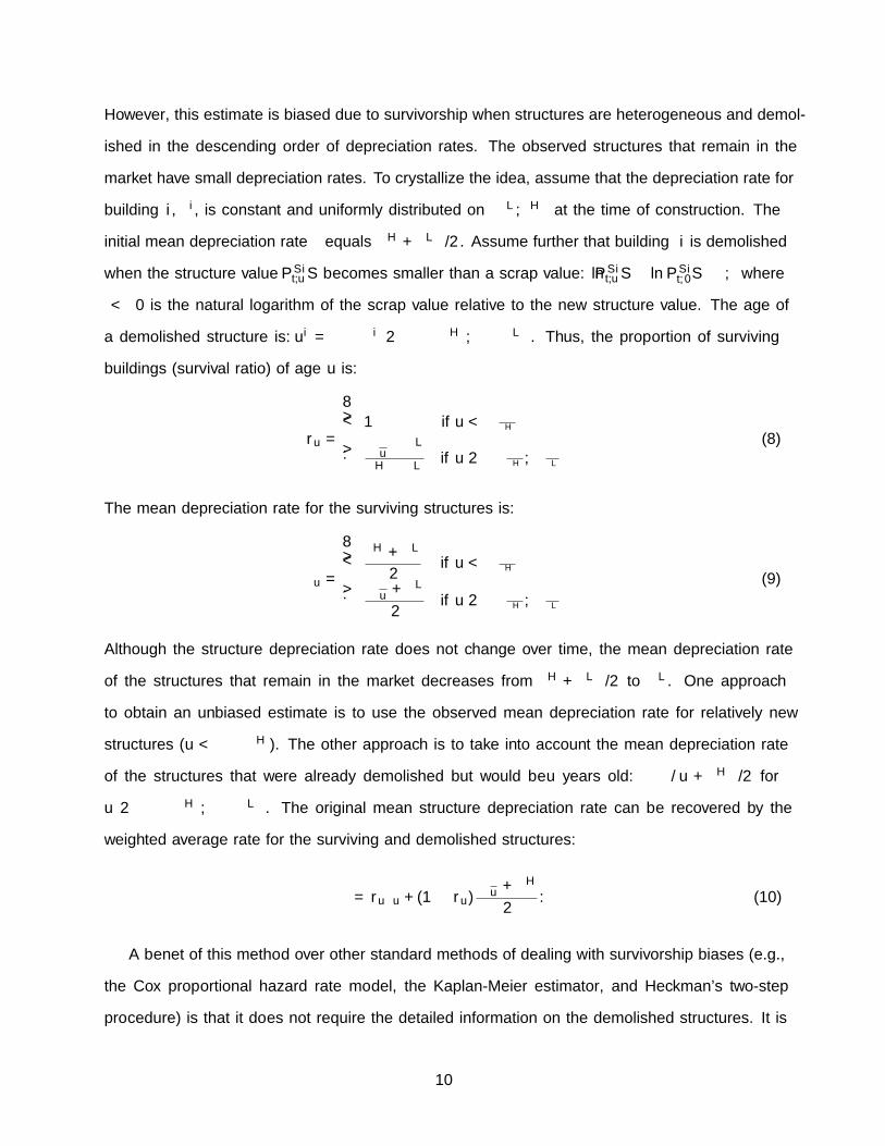
However, this estimate is biased due to survivorship when structures are heterogeneous and demol-
ished in the descending order of depreciation rates. The observed structures that remain in the
market have small depreciation rates. To crystallize the idea, assume that the depreciation rate for
building i, δi, is constant and uniformly distributed on[δL, δH
]at the time of construction. The
initial mean depreciation rate δ equals(δH + δL
)/2. Assume further that building i is demolished
when the structure value PSit,uS becomes smaller than a scrap value: lnPSit,uS − lnPSit,0S ≤ ζ, where
ζ < 0 is the natural logarithm of the scrap value relative to the new structure value. The age of
a demolished structure is: ui = −ζ/δi ∈
(−ζ/δH ,−ζ
/δL). Thus, the proportion of surviving
buildings (survival ratio) of age u is:
ru =
1 if u < − ζ
δH
− ζu − δ
L
δH − δLif u ∈
(− ζδH,− ζ
δL
) (8)
The mean depreciation rate for the surviving structures is:
δ̄u =
δH + δL
2if u < − ζ
δH
− ζu + δL
2if u ∈
(− ζδH,− ζ
δL
) (9)
Although the structure depreciation rate does not change over time, the mean depreciation rate
of the structures that remain in the market decreases from(δH + δL
)/2 to δL. One approach
to obtain an unbiased estimate is to use the observed mean depreciation rate for relatively new
structures (u < −ζ/δH ). The other approach is to take into account the mean depreciation rate
of the structures that were already demolished but would be u years old:(−ζ /u + δH
)/2 for
u ∈(−ζ/δH ,−ζ
/δL). The original mean structure depreciation rate can be recovered by the
weighted average rate for the surviving and demolished structures:
δ = ruδ̄u + (1− ru)− ζu + δH
2. (10)
A benefit of this method over other standard methods of dealing with survivorship biases (e.g.,
the Cox proportional hazard rate model, the Kaplan-Meier estimator, and Heckman’s two-step
procedure) is that it does not require the detailed information on the demolished structures. It is
10
common that data are available only for the surviving structures. The proposed method does not
need those data by imposing a structure in the distribution of depreciation rates. However, the
specific formulas (8), (9), and (10) depend on the distributional assumption.
The proposed method is somewhat similar to the method proposed by Hulten and Wykoff
(1981b) in that both methods take a weighted average for the surviving and demolished structures,
there is an important difference. They take the weighted average of structure values by assuming
that the value of demolished structures is always zero. Thus, they implicitly assume that the change
in the value of demolished structures is zero. In contrast, I recover the mean depreciation rate if
all structures existed by taking the weighted average of depreciation rates. In other words, the
method in this study incorporates large depreciation rates of demolished structures.
C. Bias Corrections: Case of Demolition Data
Consider the model characterized by equations (8) and (9). There is a one-to-one relationship
between a depreciation rate δi and the age at demolition ui (i.e., building life): ui = −ζ/δi .
Suppose the initial depreciation rate is drawn from a continuous probability density function f(δi)
on the support [δL, δH ]. Then the corresponding life span is distributed on [−ζ/δH ,−ζ
/δL ].
At any time t, a full range of depreciation rates (and life spans) are observed in the sample of
demolished structures.
However, since structures with a short life (i.e., a large depreciation rate) are frequently de-
molished, the demolition sample overrepresents these short-lived structures. If the market is in a
steady state in the sense that the total amout of structures is constant over time, the frequency
of demolition is inversely proportional to life span and directly proportional to depreciation rate.
This causes the selection bias in the observed rate of depreciation in the demolition sample. This
bias can be corrected by multiplying the probability density function of observed depreciation rate
g(δ) by u(δ) and normalize it so that its integral equals unity:
g∗(δ) ≡ g(δ)u(δ)∫ δHδL g(θ)u(θ)dθ
. (11)
When the construction volume changes over time, let Cu denote the construction volume for
age u. Then, in the time t sample of demolished structures, the frequency of age u is proportional
11

to Cu. This causes the second bias in the observed depreciation rate in a demolition sample. This
bias can be corrected by multiplying the probability density function and normalizing it. Thus, the
density function corrected for both biases is:
g∗∗(δ) ≡g(δ)u(δ)C−1
u(δ)∫ δHδL g(θ)u(θ)C−1
u(θ)dθ. (12)
III. Data
This study uses three different data sets. The first data set contains transactions of single-
family housing in Centre County, PA in the United States. The data is taken from the Multiple
Lisiting Service (MLS) data between 1996 and 2015. Centre County comprises the State College
Metropolitan Statistical Area where the Pennsylvania State University’s main campus is located.
The population was 153,990 in the 2010 Census. Although it is a college town, it has a well-balanced
industry structure, which approximately represents the national average. For example, the largest
value of location quotient is only 1.33 for real estate, rental and leasing.8
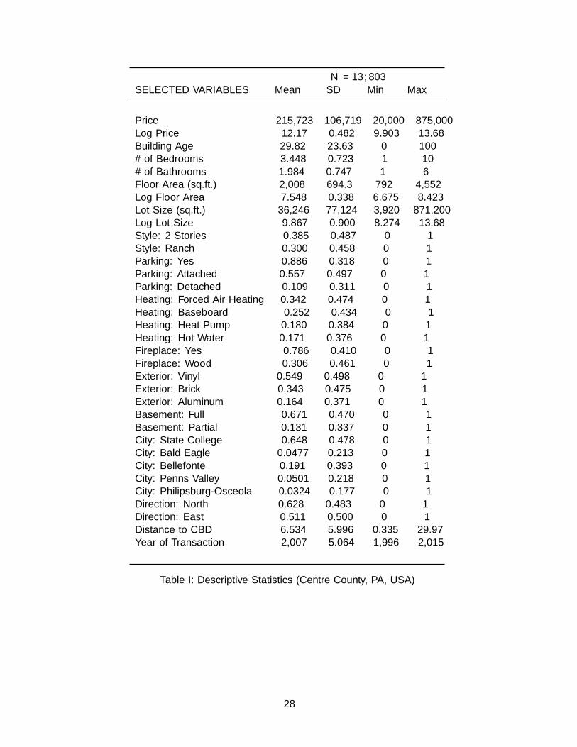
Table I shows the descriptive statistics. The average home price is $215,723, which approxi-
mately equals the national average during the sample period. The average characteristics of houses
are 30 years old, 2,000 square feet of floor area, 36,000 square feet of lot size, and 6.5 miles from
the CBD. Houses typically have 2 stories, a parking structure, a fireplace, Vinyl exterior, and a
basement.
The second data set contains transactions of the Japanese residential and commercial properties
between 2005 and 2007 compiled by Yoshida, Yamazaki, and Lee (2009). The original source is the
Transaction Price Information Service (TPIS) obtained from the Ministry of Land, Infrastructure,
Transport, and Tourism (MLIT). The MLIT generates its data by combining three data sources.
First, the registry data are obtained from the Ministry of Justice (MOJ) on transactions of raw
land, built property, and condominiums. The MOJs registry information includes location, plot
number, land use type, area, dates of receipt and contract, and the name and address of the new
owner. Second, property buyers fill out the MLIT survey on the transaction price, property size,
and reason for the transaction. Third, real estate appraisers conduct a field survey on each property
8The location quotient is the ratio of an industrys share of regional employment to its share of national employment.See www.bls.gov/cew/cewlq.htm.
12
to record the information necessary to perform an appraisal, such as building height, frontal road,
distance from the nearest railway station, site shape, and land use. The TPIS is the only source
of transaction price data and is regarded as the most reliable price data by real estate appraisers.
Since the data set contains a rich set of real estate characteristics, hedonic models have a significant
explanatory power.
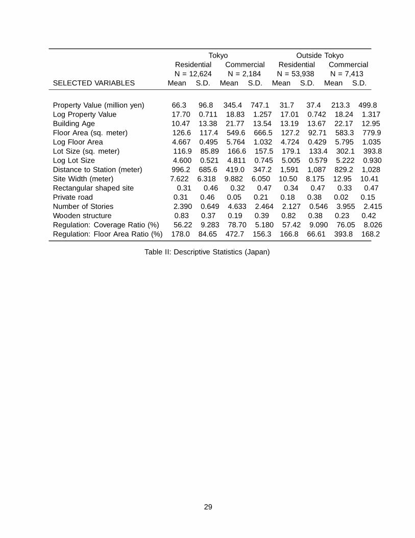
Table II shows the descriptive statistics of major variables used in the empirical analysis. I divide
the sample to Tokyo and Non-Tokyo to characterize large and small cities. I removed outliers in
terms of the number of stories, sales price, price per floor area, floor area, lot size, age, and the
distance to the CBD. The number of residential transactions is 12,624 and 53,938 for Tokyo and
elsewhere, respectively. The number of commercial transactions is 2,184 and 7,413, respectively.
The average transaction price for residential real estate is 66 million yen for Tokyo and 32 million
yen for outside Tokyo. The average price is significantly larger for commercial real estate: 345
million yen for Tokyo and 213 million yen for outside Tokyo. The average age of structures is
10-13 years for residential and 21-22 years for commercial real estate. The average floor area is
approximately 127 m2 for residential and 550 m2 for commercial real estate. Residential properties
typically have one- or two-story wooden structures and are located in a residential zoning area
with low floor-to-area ratio (FAR). Commercial properties typically have non-wooden structures
of 4-story or higher and are located in a commercial zoning area with a large FAR near a train
station. Most sites have a regular shape and face public roads.
The third data set is the demolition statistics constructed from two data sources. The first
data source is the Annual Survey on Capital Expenditures and Disposals of Private Enterprises
in the system of National Accounts of Japan. This survey is conducted by the Cabinet Office
of Japan since 2005 and considered one of a few reliable statistics of asset demolition. In the
most recent survey, 13,524 firms reported their actual capital expenditures and disposals. The
statistics include the number of demolished structures by ten age groups for single-family housing,
apartment, factory, warehouse, office, hotel, restaurant, and retail. I use surveys between 2005 and
2014, which contain 1,351 residential, 15,782 industrial, 8,531 office, 383 hotel, and 6,141 retail
properties. The second data source is buildings construction started (construction starts) from the
Annual Survey on Construction Statistics conducted by the MLIT. This survey is based on the
mandated construction registration information and goes back to 1951. The construction volume
13
in the past is used to correct for estimation biases.
IV. Empirical Strategy
I analyze five samples for (1) residential properties in Centre County, PA, USA, (2) residential
properties in Tokyo, (3) residential properties outside Tokyo in Japan, (4) commercial properties
in Tokyo, and (5) commercial properties outside Tokyo in Japan. For each sample, I estimate the
following hedonic model:
lnVijt =a0 + f(Ai, lnSi, lnLi, Di)
+ a2 lnSi + a3 (lnSi)2 + a4 lnLi + a5 (lnLi)
2 + a6Di + a7D2i + a8D
3i
+ a9 lnSi × lnLi + a10 lnSi ×Di + a11 lnLi ×Di
+Xib+Nj +Qt + εit, (13)
where Vijt denotes the price of property i located in district j traded in time t, lnSi denotes the
log floor area, Li denotes the log lot size, Di denotes the distance, f(Ai, lnSi, lnLi, Di) denotes a
function of building age Ai and its interaction terms with the above variables, and εit denotes the
error term. The location fixed effects Nj are school districts for Centre County, wards and cities for
Tokyo, and prefectures for the other part of Japan. The time fixed effects Qt are years for Centre
County and quarters for Japan.9 The vector Xi includes a rich set of property characteristics:
For Centre County, the number of bathrooms, building style, parking, heating system, exterior
finish, and basement; for Japan, the site shape, street type, rental or non-rental, structure type,
the number of stories, zoning, the FAR restriction, the building coverage ratio restriction for Japan.
Tables I and II show the descriptive statistics of major variables.
The translog function with respect to land and structure provides flexibility in the estimation
(See Rosen, 1978). The marginal effects of the log floor area (∂ lnVijt /∂ lnSi ) and the log lot
size (∂ lnVijt /∂ lnLi ) represent the structure value share and the land value share, respectively
(equations (5) and (6)). I use these shares to estimate the structure depreciation rate (equation
(7)).
9The coefficients on Qt form a hedonic price index (e.g., Ito and Hirono, 1993; Yoshida, Yamazaki, and Lee, 2009),but it is not a focus of the present study.
14
The property depreciation rate is measured by the marginal effect of building age (∂f /∂Ai ). I
first estimate the non-parametric function f(Ai) without interaction terms. To include interaction
terms, I use a step function of age groups as a parametric counterpart of this function. Specifically,
I estimate:
f(Ai, lnSi, lnLi, Di) =∑g
a1,gIg + a1,g,sIg × lnSi + a1,g,lIg × lnLi + a1,g,dIg ×Di, (14)
where Ig is an indicator function for the 5-year or 10-year age group g. I also estimate the following
parametric models to directly obtain the annual depreciation rate:
f(Ai) = a1Ai, (15)
f(Ai, lnSi, lnLi, Di) =∑g
a1,gAiIg + a1,sAi lnSi + a1,lAi lnLi + a1,dAiDi. (16)
In particular, the additional interaction term with distance can be important because of a correla-
tion between distance and building age. The new houses were actively developed around the city
center a century ago but at more distant locations in later years as the city size grew. Figure 13 in
Appendix A depicts how the active development areas changed over time.
V. The Cross-Sectional Variation in Property Depreciation
Rates
A. Japan
Figures 1 through 4 depict the estimated depreciation profiles for residential and commercial
properties in Japan. Panel (a) shows the nonparametric estimate of relative prices for different ages.
The graph is truncated at 50 years old because the number of older properties is small and standard
errors are very large. The depreciation profile in Japan exhibits both similarities and differences
compared with that for the United States. First, the functional form is generally similar until 50
years old. In particular, property values level off by 50 years old. However, unlike in the U.S.,
the depreciation rate is very small for the first few years before it increases and remains high for
the subsequent 15 years. Overall, the total depreciation is large in Japan; for example, residential
15
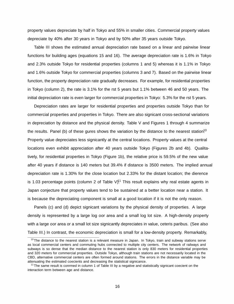
property values depreciate by half in Tokyo and 55% in smaller cities. Commercial property values
depreciate by 40% after 30 years in Tokyo and by 50% after 35 years outside Tokyo.
Table III shows the estimated annual depreciation rate based on a linear and pairwise linear
functions for building ages (equations 15 and 16). The average depreciation rate is 1.6% in Tokyo
and 2.3% outside Tokyo for residential properties (columns 1 and 5) whereas it is 1.1% in Tokyo
and 1.6% outside Tokyo for commercial properties (columns 3 and 7). Based on the pairwise linear
function, the property depreciation rate gradually decreases. For example, for residential properties
in Tokyo (column 2), the rate is 3.1% for the first 5 years but 1.1% between 46 and 50 years. The
initial depreciation rate is even larger for commercial properties in Tokyo: 5.3% for the first 5 years.
Depreciation rates are larger for residential properties and properties outside Tokyo than for
commercial properties and properties in Tokyo. There are also significant cross-sectional variations
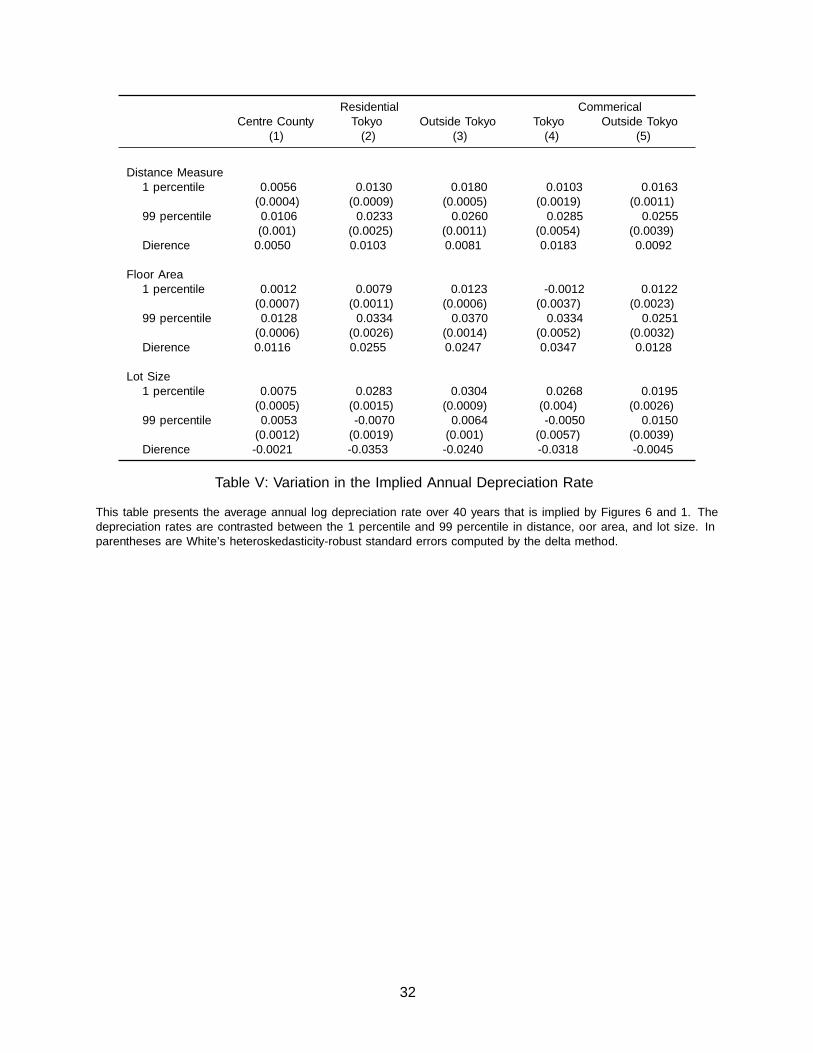
in depreciation by distance and the physical density. Table V and Figures 1 through 4 summarize
the results. Panel (b) of these figures shows the variation by the distance to the nearest station.10
Property value depreciates less significantly at the central locations. Property values at the central
locations even exhibit appreciation after 40 years outside Tokyo (Figures 2b and 4b). Qualita-
tively, for residential properties in Tokyo (Figure 1b), the relative price is 59.5% of the new value
after 40 years if distance is 140 meters but 39.4% if distance is 3500 meters. The implied annual
depreciation rate is 1.30% for the close location but 2.33% for the distant location; the difference
is 1.03 percentage points (column 2 of Table V).11 This result explains why real estate agents in
Japan conjecture that property values tend to be sustained at a better location near a station. It
is because the depreciating component is small at a good location if it is not the only reason.
Panels (c) and (d) depict significant variations by the physical density of properties. A large
density is represented by a large log floor area and a small log lot size. A high-density property
with a large floor area or a small lot size significantly depreciates in value, ceteris paribus. (See also
Table III.) In contrast, the economic depreciation is small for a low-density property. Remarkably,
10The distance to the nearest station is a relevant measure in Japan. In Tokyo, train and subway stations serveas local commercial centers and commuting hubs connected to multiple city centers. The network of railways andsubways is so dense that the median distance to the nearest station is only 830 meters for residential propertiesand 320 meters for commercial properties. Outside Tokyo, although train stations are not necessarily located in theCBD, alternative commercial centers are often formed around stations. The errors in the distance variable may beattenuating the estimated coefficients and decreasing the statistical significance.
11The same result is confirmed in column 1 of Table III by a negative and statistically significant coefficient on theinteraction term between age and distance.
16
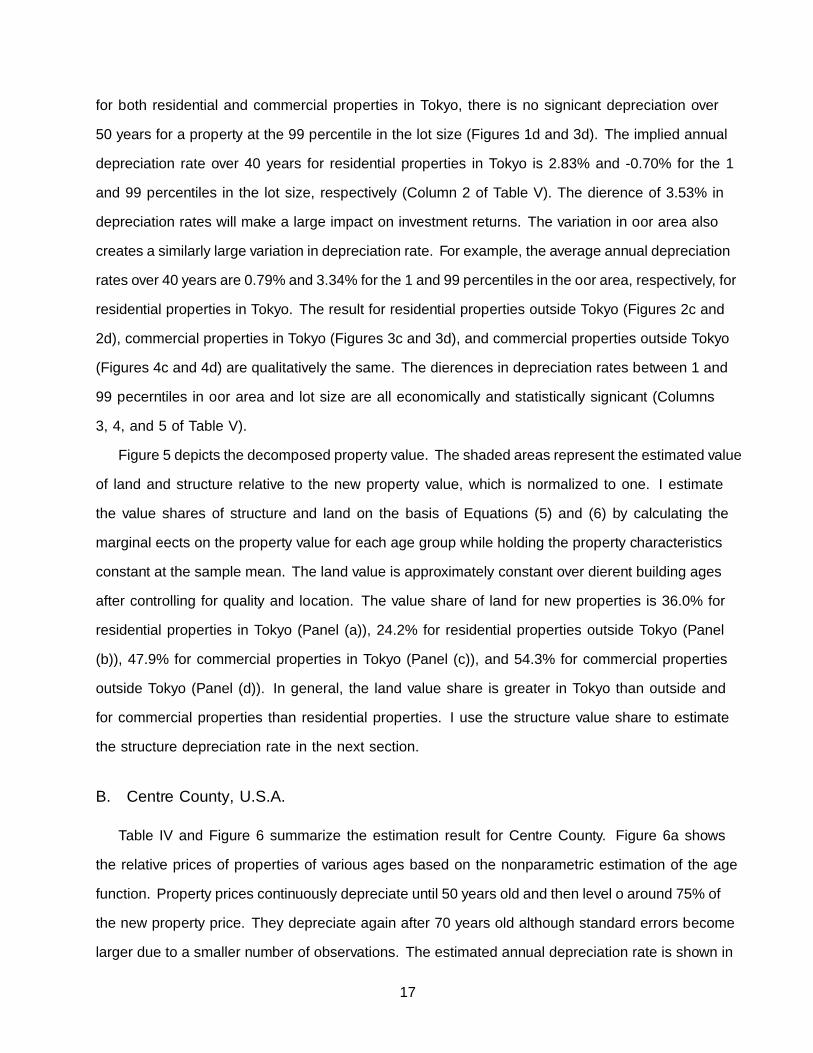
for both residential and commercial properties in Tokyo, there is no significant depreciation over
50 years for a property at the 99 percentile in the lot size (Figures 1d and 3d). The implied annual
depreciation rate over 40 years for residential properties in Tokyo is 2.83% and -0.70% for the 1
and 99 percentiles in the lot size, respectively (Column 2 of Table V). The difference of 3.53% in
depreciation rates will make a large impact on investment returns. The variation in floor area also
creates a similarly large variation in depreciation rate. For example, the average annual depreciation
rates over 40 years are 0.79% and 3.34% for the 1 and 99 percentiles in the floor area, respectively, for
residential properties in Tokyo. The result for residential properties outside Tokyo (Figures 2c and
2d), commercial properties in Tokyo (Figures 3c and 3d), and commercial properties outside Tokyo
(Figures 4c and 4d) are qualitatively the same. The differences in depreciation rates between 1 and
99 pecerntiles in floor area and lot size are all economically and statistically significant (Columns
3, 4, and 5 of Table V).
Figure 5 depicts the decomposed property value. The shaded areas represent the estimated value
of land and structure relative to the new property value, which is normalized to one. I estimate
the value shares of structure and land on the basis of Equations (5) and (6) by calculating the
marginal effects on the property value for each age group while holding the property characteristics
constant at the sample mean. The land value is approximately constant over different building ages
after controlling for quality and location. The value share of land for new properties is 36.0% for
residential properties in Tokyo (Panel (a)), 24.2% for residential properties outside Tokyo (Panel
(b)), 47.9% for commercial properties in Tokyo (Panel (c)), and 54.3% for commercial properties
outside Tokyo (Panel (d)). In general, the land value share is greater in Tokyo than outside and
for commercial properties than residential properties. I use the structure value share to estimate
the structure depreciation rate in the next section.
B. Centre County, U.S.A.
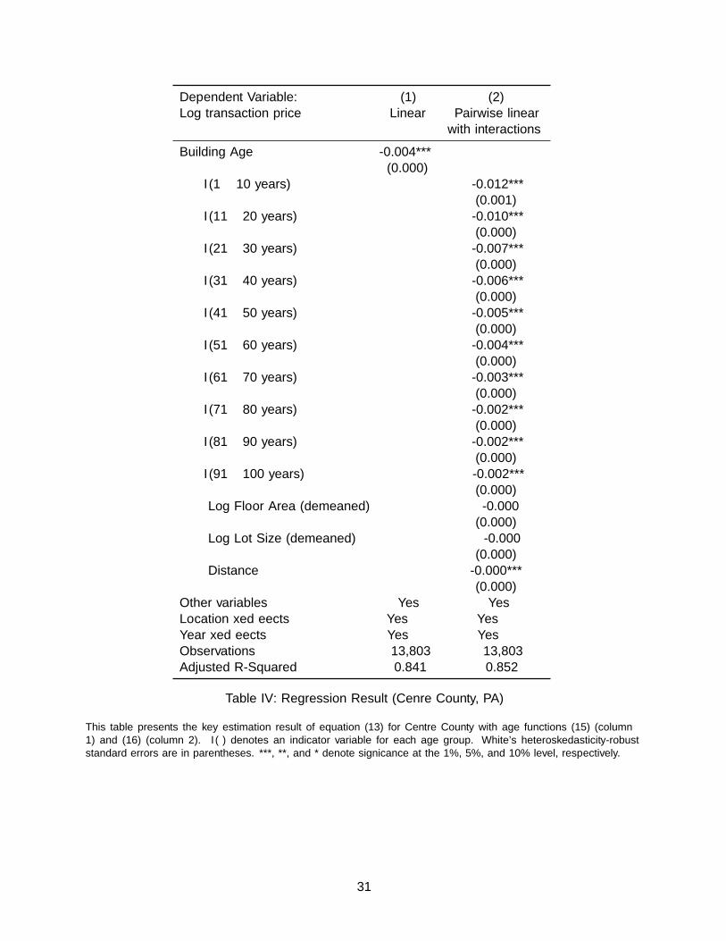
Table IV and Figure 6 summarize the estimation result for Centre County. Figure 6a shows
the relative prices of properties of various ages based on the nonparametric estimation of the age
function. Property prices continuously depreciate until 50 years old and then level off around 75% of
the new property price. They depreciate again after 70 years old although standard errors become
larger due to a smaller number of observations. The estimated annual depreciation rate is shown in
17
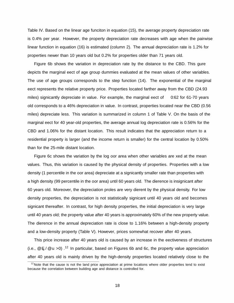
Table IV. Based on the linear age funciton in equation (15), the average property depreciation rate
is 0.4% per year. However, the property depreciation rate decreases with age when the pairwise
linear function in equation (16) is estimated (column 2). The annual depreciation rate is 1.2% for
properties newer than 10 years old but 0.2% for properties older than 71 years old.
Figure 6b shows the variation in depreciation rate by the distance to the CBD. This figure
depicts the marginal effect of age group dummies evaluated at the mean values of other variables.
The use of age groups corresponds to the step function (14). The exponential of the marginal
effect represents the relative property price. Properties located farther away from the CBD (24.93
miles) significantly depreciate in value. For example, the marginal effect of −0.62 for 61-70 years
old corresponds to a 46% depreciation in value. In contrast, properties located near the CBD (0.56
miles) depreciate less. This variation is summarized in column 1 of Table V. On the basis of the
marginal effect for 40 year-old properties, the average annual log depreciation rate is 0.56% for the
CBD and 1.06% for the distant location. This result indicates that the appreciation return to a
residential property is larger (and the income return is smaller) for the central location by 0.50%
than for the 25-mile distant location.
Figure 6c shows the variation by the log floor area when other variables are fixed at the mean
values. Thus, this variation is caused by the physical density of properties. Properties with a low
density (1 percentile in the floor area) depreciate at a significantly smaller rate than properties with
a high density (99 percentile in the floor area) until 60 years old. The difference is insignificant after
60 years old. Moreover, the depreciation profiles are very different by the physical density. For low
density properties, the depreciation is not statistically significant until 40 years old and becomes
significant thereafter. In contrast, for high density properties, the initial depreciation is very large
until 40 years old; the property value after 40 years is approximately 60% of the new property value.
The difference in the annual depreciation rate is close to 1.16% between a high-density property
and a low-density property (Table V). However, prices somewhat recover after 40 years.
This price increase after 40 years old is caused by an increase in the effectiveness of structures
(i.e., ∂Eu /∂u > 0) .12 In particular, based on Figures 6b and 6c, the property value appreciation
after 40 years old is mainly driven by the high-density properties located relatively close to the
12Note that the cause is not the land price appreciation at prime locations where older properties tend to existbecause the correlation between building age and distance is controlled for.
18
CBD. Other types of properties constantly depreciate in value with age. On the basis of the
theoretical model, the value appreciation for old properties can be caused either by increasing
prices of the effective structure (PES) or the increasing effectiveness of structure (Eu). However,
it is not plausible that the price of deteriorated structures significantly increases only for high-
density properties in downtown areas. Rather, it seems more natural that the effectiveness of
structure gradually increases after 40 years due to the increasing value of renovation options or
historic qualities particularly for high-density properties located in the downtown area. However,
separating out these appreciating factors is not possible from the data of this study.
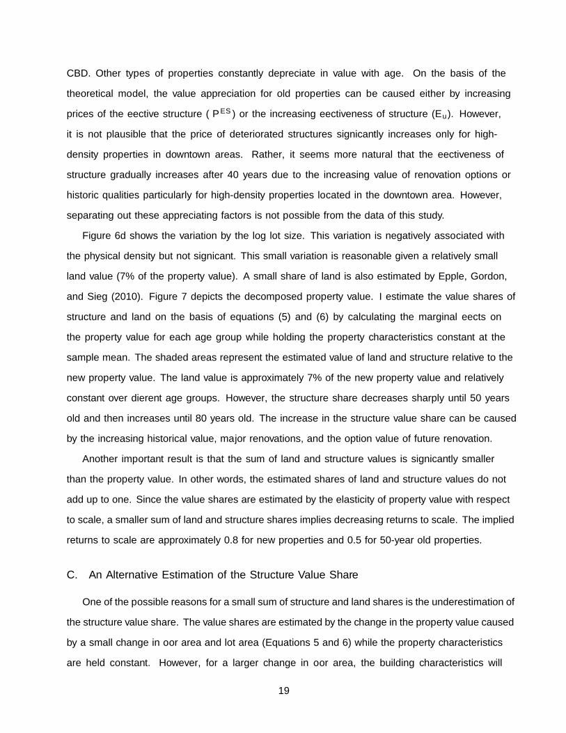
Figure 6d shows the variation by the log lot size. This variation is negatively associated with
the physical density but not significant. This small variation is reasonable given a relatively small
land value (7% of the property value). A small share of land is also estimated by Epple, Gordon,
and Sieg (2010). Figure 7 depicts the decomposed property value. I estimate the value shares of
structure and land on the basis of equations (5) and (6) by calculating the marginal effects on
the property value for each age group while holding the property characteristics constant at the
sample mean. The shaded areas represent the estimated value of land and structure relative to the
new property value. The land value is approximately 7% of the new property value and relatively
constant over different age groups. However, the structure share decreases sharply until 50 years
old and then increases until 80 years old. The increase in the structure value share can be caused
by the increasing historical value, major renovations, and the option value of future renovation.
Another important result is that the sum of land and structure values is significantly smaller
than the property value. In other words, the estimated shares of land and structure values do not
add up to one. Since the value shares are estimated by the elasticity of property value with respect
to scale, a smaller sum of land and structure shares implies decreasing returns to scale. The implied
returns to scale are approximately 0.8 for new properties and 0.5 for 50-year old properties.
C. An Alternative Estimation of the Structure Value Share
One of the possible reasons for a small sum of structure and land shares is the underestimation of
the structure value share. The value shares are estimated by the change in the property value caused
by a small change in floor area and lot area (Equations 5 and 6) while the property characteristics
are held constant. However, for a larger change in floor area, the building characteristics will
19
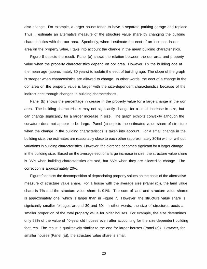
also change. For example, a larger house tends to have a separate parking garage and fireplace.
Thus, I estimate an alternative measure of the structure value share by changing the building
characteristics with the floor area. Specifically, when I estimate the effect of an increase in floor
area on the property value, I take into account the change in the mean building characteristics.
Figure 8 depicts the result. Panel (a) shows the relation between the floor area and property
value when the property characteristics depend on floor area. However, I fix the building age at
the mean age (approximately 30 years) to isolate the effect of building age. The slope of the graph
is steeper when characteristics are allowed to change. In other words, the effect of a change in the
floor area on the property value is larger with the size-dependent characteristics because of the
indirect effect through changes in building characteristics.
Panel (b) shows the percentage in crease in the property value for a large change in the floor
area. The building characteristics may not significantly change for a small increase in size, but
can change significantly for a larger increase in size. The graph exhibits convexity although the
curvature does not appear to be large. Panel (c) depicts the estimated value share of structure
when the change in the building characteristics is taken into account. For a small change in the
building size, the estimates are reasonably close to each other (approximately 30%) with or without
variations in building characteristics. However, the difference becomes significant for a larger change
in the building size. Based on the average effect of a large increase in size, the structure value share
is 35% when building characteristics are fixed, but 55% when they are allowed to change. The
correction is approximately 20%.
Figure 9 depicts the decomposition of depreciating property values on the basis of the alternative
measure of structure value share. For a house with the average size (Panel (b)), the land value
share is 7% and the structure value share is 91%. The sum of land and structure value shares
is approximately one, which is larger than in Figure 7. However, the structure value share is
significantly smaller for ages around 30 and 60. In other words, the size of structures affects a
smaller proportion of the total property value for older houses. For example, the size determines
only 58% of the value of 40-year old houses even after accounting for the size-dependent building
features. The result is qualitatively similar to the one for larger houses (Panel (c)). However, for
smaller houses (Panel (a)), the structure value share is small.
20
VI. Bias-Corrected Rates of Structure Depreciation
This section empirically demonstrates two bias adjustment methods that I propose. The first
method (Section II.B) is applied to the property depreciation rate estimated by hedonic regressions
of traded real estate prices. The second method (Section II.C) is applied to the demolition statistics.
A. Asset Price Approach
I estimate the bias-corrected rate of structure depreciation by using equations 7 and 10. The
data for this exercise are summarized in Tables VII and VI. For the annual property depreciation
rate, I use the estimate of the pairwise linear function (16) (Tables IV and III). The structure value
share is taken from the result depicted in Figures 5 and 7. To calculate survival ratio, I set the lower
bound of structure depreciation rate as half of the initial depreciation rate. For Japan, I set the the
lower and upper bounds such that the implied survival rates approximately match the demolition
data (column 5 of Table VI). Note that these upper and lower bounds affect the variances but not
the mean depreciation rate. The scrap value of structure is 20% of the original value: ζ = ln 0.2.
Figure 10 depicts the estimation result. Downward-sloping dashed lines are property depreci-
ation rates estimated by hedonic regressions whereas the thick solid lines are the bias corrected
structure depreciation rates for each age group. The property depreciation rates are smaller than
the structure depreciation rates due to both the effect of structure value share and a survivorship
bias. In the United States, the structure depreciation rate is small and decreasing with age; the
initial depreciation rate is 1.8%, but the rate for old buildings is 0.3%. Because the building life is
relatively long, the survivorship bias is not large. Furthermore, since the structure value share is
large in Centre County, PA, its effect is also small.
In contrast, the structure depreciation rate is much larger in Japan. For residential properties,
the initial depreciation rate is 5.8% in Tokyo and 6.7% outside Tokyo. These rates tend to increase
with age and become 7.7% in Tokyo and 7.3% outside Tokyo. For commercial properties, the initial
depreciation rate is 10.8% in Tokyo and 9.8% outside Tokyo. These rates do not change much with
age and become 10.0% and 9.1%, respectively, after 50 years. The median age group is 26-35 years
for residential properties and 16-25 years for commercial properties. At the median age, the bias-
corrected aggregate structure depreciation rate is 6.4% for residential properties in Tokyo, 7.0%
21
for residential properties outside Tokyo, 10.2% for commercial properties in Tokyo, and 9.1% for
commercial properties outside Tokyo. These rates fall in the range of the lowest estimate by Seko
(1998) and the highest estimate by Yoshida and Ha (2001). These rates are also significantly larger
than those in the United States.
B. Demolition Approach
The sample of demolished structures is another source of information for depreciation rates.
Since the life span of a structure is directly associated with its depreciation rate, one can infer
the depreciation rate by measuring the building age at the time of demolition. However, there are
obvious biases because the sample of demolished structures do not represent the entire population of
structures. The first is a selection bias that fast depreciating structures are more frequently observed
in the sample of demolished structures. The second bias is that historical changes in construction
volume affect the age distribution of demolished buildings. For example, a construction boom that
occurred several decades ago would naturally increases the frequency of the corresponding ages in
the current demolition sample.
Figure 11 depicts the cumulative distribution of building age at demolition. The ten age groups
in the data are on the horizontal axis. Panel (a) shows unadjusted distributions by property type.
Residential real estate has the longest life and retail real estate has the shortest life. The observed
median life is quite short: 30-40 years for residential, 20-25 years for industrial, 15-20 years for
office, 10-15 years for hotel, and 5-10 years for retail. However, by adjusting for frequency and
construction volume, the cumulative distribution function tends to be shifted to the right (Panels
b and c). The median life corrected for both biases (Panel c) is 40-50 years for residential, 25-30
years for industrial and office, 15-20 years for hotel, and 20-25 years for retail.
Figure 12 depicts the probability mass function for depreciation rates. The discrete depreciation
rates on the horizontal axis correspond to ten age groups. Panels (a), (b), and (c) are discrete
analogues of density functions g(δ), g∗(δ), and g∗∗(δ), respectively. By comparing Panel (a) with
Panel (c), it is clear that probability masses are shifted toward smaller depreciation rates. The
shift is most clearly seen for residential and retail. The residential distribution is extremely skewed
to the right after correcting for biases. The unadjusted retail distribution is skewed to the left but
the adjusted distribution is more symmetrical.
22
Table VIII presents the mean and median depreciation rate with and without bias corrections by
Equation (12). Since these rates depend on the assumption of scrap value, I examine three cases of
scrap value. First, bias corrections are significant in magnitude. For example, when the scrap value
equals 0.15, the unadjusted mean depreciation rate for residential real estate is 9.64% whereas the
bias-corrected rate is 6.20%. The unadjuted rates are unreasonably large; e.g., 28.82% for retail.
Second, the bias-corrected mean depreciation rate is consistent with the rate estimated by the asset
price approach when the scrap value equals 0.15 or 0.2. For example, when the scrap value is 0.15,
the mean rate is 6.2% for residential and 9.2-17.2% for commercial real estate. Although there are
no reliable statistics for scrap values, this scrap value seems reasonable.
VII. Conclusion
This study estimates real estate depreciation rates both at the property-level and teh structure-
level. The outcome of this study has several important implications. First, the cross-sectional
variation in the property depreciation rate has an important implication on real estate investments
and the housing economics. Second, the bias corrected structure depreciation rate serves as an
important input to macroeconomics models.
The result is qualitatively summarized as follows. The property depreciation rate decreases
with age and is always smaller than the structure depreciation rate due to the effect of the non-
depreciating land component and a survivorship bias. The property depreciation rate is larger
for newer and denser properties located away from the CBD in a smaller city. The structure
depreciation rate is larger in Japan than in the U.S. and larger for commercial properties than for
residential properties.
23
References
Alonso, William, 1964, Location and Land Use; Toward a General Theory of Land Rent (Harvard
University Press: Cambridge, MA).
Ambrose, Brent W., N. Edward Coulson, and Jiro Yoshida, 2015, The repeat rent index, Review
of Economics and Statistics.
Cabinet Office of Japan, 2013, White paper on disaster management, Discussion paper.
Coulson, N. Edward, and Daniel P. McMillen, 2008, Estimating time, age and vintage effects in
housing prices, Journal of Housing Economics 17, 138 – 151.
Davidoff, Thomas, and Jiro Yoshida, 2013, Estimating consumption substitution between housing
and non-housing goods using macro data, Working paper.
Davis, Morris, and Jonathan Heathcote, 2005, Housing and the business cycle, International Eco-
nomic Review 46, 751–784.
Davis, Morris A., and Stijn Van Nieuwerburgh, 2015, Chapter 12 - housing, finance, and the
macroeconomy, in J. Vernon Henderson Gilles Duranton, and William C. Strange, ed.: Handbook
of Regional and Urban Economics, vol. 5 of Handbook of Regional and Urban Economics . pp.
753 – 811 (Elsevier).
Dekle, Robert, and Lawrence H. Summers, 1991, Japan’s High Saving Rate Reaffirmed, NBER
Working Papers 3690 National Bureau of Economic Research, Inc.
Duranton, Gilles, and Diego Puga, 2015, Chapter 8 - urban land use, in J. Vernon Henderson
Gilles Duranton, and William C. Strange, ed.: Handbook of Regional and Urban Economics,
vol. 5 of Handbook of Regional and Urban Economics . pp. 467 – 560 (Elsevier).
Economic and Social Research Institute, 2011, Outline of the 2005 revision to the national account
(in japanese), Discussion paper Cabinet Office of Japan.
Epple, Dennis, Brett Gordon, and Holger Sieg, 2010, A new approach to estimating the production
function for housing, American Economic Review 100, 905–24.
24
Fisher, Jeffrey D., Brent C Smith, Jerrold J. Stern, and R. Brian Webb, 2005, Analysis of Economic
Depreciation for Multi-Family Property, Journal of Real Estate Research 27, 355–370.
Fujita, Masahisa, 1989, Urban Economic Theory . No. 9780521346627 in Cambridge Books (Cam-
bridge University Press).
Geltner, D., and S. Bokhari, 2015, The nature and magnitude of commercial buildings capital
consumption in the united states, Working paper MIT Center for Real Estate.
Greenwood, Jeremy, and Zvi Hercowitz, 1991, The Allocation of Capital and Time over the Business
Cycle, Journal of Political Economy 99, 1188–214.
Harding, John P., Stuart S. Rosenthal, and C.F. Sirmans, 2007, Depreciation of housing capital,
maintenance, and house price inflation: Estimates from a repeat sales model, Journal of Urban
Economics 61, 193 – 217.
Hayashi, Fumio, 1986, Why Is Japan’s Saving Rate So Apparently High?, in NBER Macroeconomics
Annual 1986, Volume 1 NBER Chapters . pp. 147–234 (National Bureau of Economic Research,
Inc).
, 1989, Japan’s Saving Rate: New Data and Reflections, NBER Working Papers 3205
National Bureau of Economic Research, Inc.
, 1991, Measuring Depreciation For Japan: Rejoinder to Dekle and Summers, NBER Work-
ing Papers 3836 National Bureau of Economic Research, Inc.
, Takatoshi Ito, and Joel Slemrod, 1987, Housing Finance Imperfections and Private Saving:
A Comparative Simulation Analysis of the U.S. and Japan, NBER Working Papers 2272 National
Bureau of Economic Research, Inc.
Hayashi, Fumio, and Edward C. Prescott, 2002, The 1990s in Japan: A Lost Decade, Review of
Economic Dynamics 5, 206–235.
Hulten, Charles, and Frank C. Wykoff, 1981a, The Measurement of Economic Depreciation, in
Charles Hulten, ed.: Depreciation, Inflation, and the Taxation of Income from Capital . pp.
81–125 (The Urban Institute, Washington, D.C.).
25

Hulten, Charles R., and Frank C. Wykoff, 1981b, The estimation of economic depreciation using
vintage asset prices, Journal of Econometrics 15, 367 – 396.
Imrohoroglu, Selahattin, Ayse Imrohoroglu, and Kaiji Chen, 2006, The Japanese Saving Rate,
American Economic Review 96, 1850–1858.
Ito, Takatoshi, and Keiko Nosse Hirono, 1993, Efficiency of the Tokyo Housing Market, Monetary
and Economic Studies 11, 1–32.
Knight, John R., and C.F. Sirmans, 1996, Depreciation, maintenance, and housing prices, Journal
of Housing Economics 5, 369 – 389.
Lane, Walter F., William C. Randolph, and Stephen A. Berenson, 1988, Adjusting the cpi shelter
index to compensate for effect of depreciation, Monthly Labor Review pp. 34–37.
Leigh, Wilhelmina A., 1980, Economic depreciation of the residential housing stock of the united
states, 1950-1970, The Review of Economics and Statistics 62, 200–206.
Mills, Edwin S., 1967, An aggregative model of resource allocation in a metropolitan area, The
American Economic Review 57, 197–210.
Muth, Richard F., 1969, Cities and housing; the spatial pattern of urban residential land use (niver-
sity of Chicago Press: Chicago, IL).
Poterba, James M., 1984, Tax subsidies to owner-occupied housing: An asset-market approach,
The Quarterly Journal of Economics 99, pp. 729–752.
Rosen, Harvey S., 1978, Estimating Inter-city Differences in the Price of Housing Services, Urban
Studies 15, 351–355.
Seko, Miki, 1998, Tochi to jutaku no keizai bunseki (Sobunsha: Tokyo, Japan).
Yamazaki, F., and T. Sadayuki, 2010, An estimation of collective action cost in condominium
reconstruction: The case of japanese condominium law, Working Paper REAL 12-T-05 The
Regional Economics Applications Laboratory, University of Illinois.
Yoshida, Atsushi, and Chun Ha, 2001, Todofuken betsu jutaku stokku no suikei, Kikan Jutaku
Tochi Keizai 39, pp. 18–27.
26
Yoshida, Jiro, and Ayako Sugiura, 2015, The effects of multiple green factors on condominium
prices, The Journal of Real Estate Finance and Economics 50, 412–437.
Yoshida, J., R. Yamazaki, and J. E. Lee, 2009, Real estate transaction prices in japan: New findings
of time-series and cross-sectional characteristics, AsRES-AREUEA Conference Proceedings.
27
N = 13, 803SELECTED VARIABLES Mean SD Min Max
Price 215,723 106,719 20,000 875,000Log Price 12.17 0.482 9.903 13.68Building Age 29.82 23.63 0 100# of Bedrooms 3.448 0.723 1 10# of Bathrooms 1.984 0.747 1 6Floor Area (sq.ft.) 2,008 694.3 792 4,552Log Floor Area 7.548 0.338 6.675 8.423Lot Size (sq.ft.) 36,246 77,124 3,920 871,200Log Lot Size 9.867 0.900 8.274 13.68Style: 2 Stories 0.385 0.487 0 1Style: Ranch 0.300 0.458 0 1Parking: Yes 0.886 0.318 0 1Parking: Attached 0.557 0.497 0 1Parking: Detached 0.109 0.311 0 1Heating: Forced Air Heating 0.342 0.474 0 1Heating: Baseboard 0.252 0.434 0 1Heating: Heat Pump 0.180 0.384 0 1Heating: Hot Water 0.171 0.376 0 1Fireplace: Yes 0.786 0.410 0 1Fireplace: Wood 0.306 0.461 0 1Exterior: Vinyl 0.549 0.498 0 1Exterior: Brick 0.343 0.475 0 1Exterior: Aluminum 0.164 0.371 0 1Basement: Full 0.671 0.470 0 1Basement: Partial 0.131 0.337 0 1City: State College 0.648 0.478 0 1City: Bald Eagle 0.0477 0.213 0 1City: Bellefonte 0.191 0.393 0 1City: Penns Valley 0.0501 0.218 0 1City: Philipsburg-Osceola 0.0324 0.177 0 1Direction: North 0.628 0.483 0 1Direction: East 0.511 0.500 0 1Distance to CBD 6.534 5.996 0.335 29.97Year of Transaction 2,007 5.064 1,996 2,015
Table I: Descriptive Statistics (Centre County, PA, USA)
28
Tokyo Outside TokyoResidential Commercial Residential CommercialN = 12,624 N = 2,184 N = 53,938 N = 7,413
SELECTED VARIABLES Mean S.D. Mean S.D. Mean S.D. Mean S.D.
Property Value (million yen) 66.3 96.8 345.4 747.1 31.7 37.4 213.3 499.8Log Property Value 17.70 0.711 18.83 1.257 17.01 0.742 18.24 1.317Building Age 10.47 13.38 21.77 13.54 13.19 13.67 22.17 12.95Floor Area (sq. meter) 126.6 117.4 549.6 666.5 127.2 92.71 583.3 779.9Log Floor Area 4.667 0.495 5.764 1.032 4.724 0.429 5.795 1.035Lot Size (sq. meter) 116.9 85.89 166.6 157.5 179.1 133.4 302.1 393.8Log Lot Size 4.600 0.521 4.811 0.745 5.005 0.579 5.222 0.930Distance to Station (meter) 996.2 685.6 419.0 347.2 1,591 1,087 829.2 1,028Site Width (meter) 7.622 6.318 9.882 6.050 10.50 8.175 12.95 10.41Rectangular shaped site 0.31 0.46 0.32 0.47 0.34 0.47 0.33 0.47Private road 0.31 0.46 0.05 0.21 0.18 0.38 0.02 0.15Number of Stories 2.390 0.649 4.633 2.464 2.127 0.546 3.955 2.415Wooden structure 0.83 0.37 0.19 0.39 0.82 0.38 0.23 0.42Regulation: Coverage Ratio (%) 56.22 9.283 78.70 5.180 57.42 9.090 76.05 8.026Regulation: Floor Area Ratio (%) 178.0 84.65 472.7 156.3 166.8 66.61 393.8 168.2
Table II: Descriptive Statistics (Japan)
29

Dep
enden
tV
ari
able
:T
okyo
Outs
ide
Tokyo
Log
transa
ctio
npri
ceR
esid
enti
al
Com
mer
ical
Res
iden
tial
Com
mer
ical
(1)
(2)
(3)
(4)
(5)
(6)
(7)
(8)
Buildin
gage
-0.0
16***
-0.0
11***
-0.0
23***
-0.0
16***
(0.0
00)
(0.0
01)
(0.0
00)
(0.0
01)
×I(
1−
5yea
rs)
-0.0
31***
-0.0
53***
-0.0
44***
-0.0
48***
(0.0
04)
(0.0
13)
(0.0
02)
(0.0
10)
×I(
6−
10
yea
rs)
-0.0
21***
-0.0
36***
-0.0
36***
-0.0
28***
(0.0
01)
(0.0
08)
(0.0
01)
(0.0
04)
×I(
11−
15
yea
rs)
-0.0
20***
-0.0
31***
-0.0
33***
-0.0
29***
(0.0
01)
(0.0
03)
(0.0
01)
(0.0
02)
×I(
16−
20
yea
rs)
-0.0
19***
-0.0
22***
-0.0
29***
-0.0
25***
(0.0
01)
(0.0
02)
(0.0
00)
(0.0
01)
×I(
21−
25
yea
rs)
-0.0
16***
-0.0
21***
-0.0
25***
-0.0
24***
(0.0
01)
(0.0
02)
(0.0
00)
(0.0
01)
×I(
26−
30
yea
rs)
-0.0
14***
-0.0
19***
-0.0
24***
-0.0
23***
(0.0
01)
(0.0
02)
(0.0
00)
(0.0
01)
×I(
31−
35
yea
rs)
-0.0
14***
-0.0
16***
-0.0
21***
-0.0
20***
(0.0
01)
(0.0
02)
(0.0
00)
(0.0
01)
×I(
36−
40
yea
rs)
-0.0
13***
-0.0
10***
-0.0
18***
-0.0
16***
(0.0
01)
(0.0
02)
(0.0
00)
(0.0
01)
×I(
41−
45
yea
rs)
-0.0
13***
-0.0
09***
-0.0
16***
-0.0
15***
(0.0
01)
(0.0
02)
(0.0
00)
(0.0
01)
×I(
46−
50
yea
rs)
-0.0
11***
-0.0
08***
-0.0
14***
-0.0
12***
(0.0
01)
(0.0
02)
(0.0
01)
(0.0
01)
×L
og
Flo
or
Are
a(d
emea
ned
)-0
.008***
-0.0
05***
-0.0
09***
-0.0
04***
(0.0
01)
(0.0
02)
(0.0
01)
(0.0
01)
×L
og
Lot
Siz
e(d
emea
ned
)0.0
12***
0.0
08***
0.0
08***
0.0
03***
(0.0
01)
(0.0
02)
(0.0
00)
(0.0
01)
×D
ista
nce
-0.0
00***
-0.0
00***
-0.0
00***
-0.0
00***
(0.0
00)
(0.0
00)
(0.0
00)
(0.0
00)
Oth
erva
riable
sY
esY
esY
esY
esY
esY
esY
esY
esL
oca
tion
fixed
effec
tsY
esY
esY
esY
esY
esY
esY
esY
esY
ear-
quart
erfixed
effec
tsY
esY
esY
esY
esY
esY
esY
esY
esO
bse
rvati
ons
12,6
24
12,6
24
2,1
84
2,1
84
53,9
38
53,9
38
7,4
13
7,4
13
Adju
sted
R-s
quare
d0.8
16
0.8
26
0.8
36
0.8
44
0.6
79
0.6
98
0.7
95
0.8
00
Tab
leII
I:R
egre
ssio
nR
esu
lt(J
apan
)
This
table
pre
sents
the
key
esti
mati
on
resu
ltof
equati
on
(13)
for
Tokyo
(colu
mns
1-4
)and
outs
ide
Tokyo
(colu
mns
5-8
),fo
rb
oth
resi
den
tial
(colu
mns
1,2
,5,6
)and
com
mer
ical
(colu
mns
3,4
,7,8
)w
ith
age
funct
ions
(15)
(colu
mns
1,
3,
5,
7)
and
(16)
(colu
mns
2,
4,
6,
8).
I(·)
den
ote
san
indic
ato
rva
riable
for
each
age
gro
up.
Whit
e’s
het
erosk
edast
icit
y-r
obust
standard
erro
rsare
inpare
nth
eses
.***,
**,
and
*den
ote
signifi
cance
at
the
1%
,5%
,and
10%
level
,re
spec
tivel
y.
30
Dependent Variable: (1) (2)Log transaction price Linear Pairwise linear
with interactions
Building Age -0.004***(0.000)
×I(1− 10 years) -0.012***(0.001)
×I(11− 20 years) -0.010***(0.000)
×I(21− 30 years) -0.007***(0.000)
×I(31− 40 years) -0.006***(0.000)
×I(41− 50 years) -0.005***(0.000)
×I(51− 60 years) -0.004***(0.000)
×I(61− 70 years) -0.003***(0.000)
×I(71− 80 years) -0.002***(0.000)
×I(81− 90 years) -0.002***(0.000)
×I(91− 100 years) -0.002***(0.000)
× Log Floor Area (demeaned) -0.000(0.000)
× Log Lot Size (demeaned) -0.000(0.000)
× Distance -0.000***(0.000)
Other variables Yes YesLocation fixed effects Yes YesYear fixed effects Yes YesObservations 13,803 13,803Adjusted R-Squared 0.841 0.852
Table IV: Regression Result (Cenre County, PA)
This table presents the key estimation result of equation (13) for Centre County with age functions (15) (column1) and (16) (column 2). I(·) denotes an indicator variable for each age group. White’s heteroskedasticity-robuststandard errors are in parentheses. ***, **, and * denote significance at the 1%, 5%, and 10% level, respectively.
31
Residential CommericalCentre County Tokyo Outside Tokyo Tokyo Outside Tokyo
(1) (2) (3) (4) (5)
Distance Measure1 percentile 0.0056 0.0130 0.0180 0.0103 0.0163
(0.0004) (0.0009) (0.0005) (0.0019) (0.0011)99 percentile 0.0106 0.0233 0.0260 0.0285 0.0255
(0.001) (0.0025) (0.0011) (0.0054) (0.0039)Difference 0.0050 0.0103 0.0081 0.0183 0.0092
Floor Area1 percentile 0.0012 0.0079 0.0123 -0.0012 0.0122
(0.0007) (0.0011) (0.0006) (0.0037) (0.0023)99 percentile 0.0128 0.0334 0.0370 0.0334 0.0251
(0.0006) (0.0026) (0.0014) (0.0052) (0.0032)Difference 0.0116 0.0255 0.0247 0.0347 0.0128
Lot Size1 percentile 0.0075 0.0283 0.0304 0.0268 0.0195
(0.0005) (0.0015) (0.0009) (0.004) (0.0026)99 percentile 0.0053 -0.0070 0.0064 -0.0050 0.0150
(0.0012) (0.0019) (0.001) (0.0057) (0.0039)Difference -0.0021 -0.0353 -0.0240 -0.0318 -0.0045
Table V: Variation in the Implied Annual Depreciation Rate
This table presents the average annual log depreciation rate over 40 years that is implied by Figures 6 and 1. Thedepreciation rates are contrasted between the 1 percentile and 99 percentile in distance, floor area, and lot size. Inparentheses are White’s heteroskedasticity-robust standard errors computed by the delta method.
32

Age Property Depreciation Structure Value Structure Depreciation Survival Rate Structure DepreciationGroup Rate Ratio Rate without (Eq. 12) Rate with
Correction (Eq. 11) Correction (Eq. 14)
(a) Residential Properties, Tokyo. Assumptions: ζ = ln 0.2, δL = 0.005, δH = 0.1115 0.031 0.519 0.058 1.000 0.05810 0.021 0.476 0.049 1.000 0.04915 0.020 0.433 0.056 1.000 0.05620 0.019 0.390 0.045 0.866 0.05225 0.016 0.347 0.042 0.674 0.05830 0.014 0.304 0.045 0.551 0.06335 0.014 0.261 0.047 0.466 0.06540 0.013 0.218 0.062 0.404 0.07145 0.013 0.175 0.050 0.357 0.06650 0.011 0.132 0.086 0.319 0.077
(b) Residential Properties, Outside Tokyo. Assumptions: ζ = ln 0.2, δL = 0.005, δH = 0.1305 0.044 0.718 0.067 1.000 0.06710 0.036 0.671 0.054 1.000 0.05415 0.033 0.625 0.055 1.000 0.05520 0.029 0.579 0.044 0.738 0.06125 0.025 0.532 0.046 0.574 0.06930 0.024 0.486 0.044 0.469 0.07135 0.021 0.440 0.042 0.397 0.07140 0.018 0.393 0.049 0.344 0.07445 0.016 0.347 0.054 0.304 0.07550 0.014 0.301 0.049 0.272 0.073
(c) Commerical Properties, Outside Tokyo. Assumptions: ζ = ln 0.2, δL = 0.02, δH = 0.1975 0.053 0.429 0.108 1.000 0.10810 0.036 0.403 0.129 1.000 0.12915 0.031 0.377 0.086 0.728 0.10720 0.022 0.351 0.062 0.520 0.10225 0.021 0.324 0.052 0.405 0.10130 0.019 0.298 0.062 0.331 0.10635 0.016 0.272 0.059 0.280 0.10540 0.010 0.245 0.061 0.243 0.10545 0.009 0.219 0.041 0.214 0.10150 0.008 0.193 0.034 0.192 0.100
(d) Commerical Properties, Outside Tokyo. Assumptions: ζ = ln 0.2, δL = 0.02, δH = 0.1765 0.048 0.477 0.098 1.000 0.09810 0.028 0.456 0.058 1.000 0.05815 0.029 0.436 0.071 0.824 0.08620 0.025 0.415 0.058 0.589 0.08925 0.024 0.395 0.054 0.458 0.09230 0.023 0.375 0.056 0.375 0.09435 0.020 0.354 0.066 0.317 0.09840 0.016 0.334 0.047 0.275 0.09245 0.015 0.313 0.049 0.243 0.09350 0.012 0.293 0.042 0.217 0.091
Table VI: Bias-Corrected Rate of Structure Depreciation (Japan)
This table presents the bias correction in the estimation of the structure depreciation rate based on equations 7 and10.
33
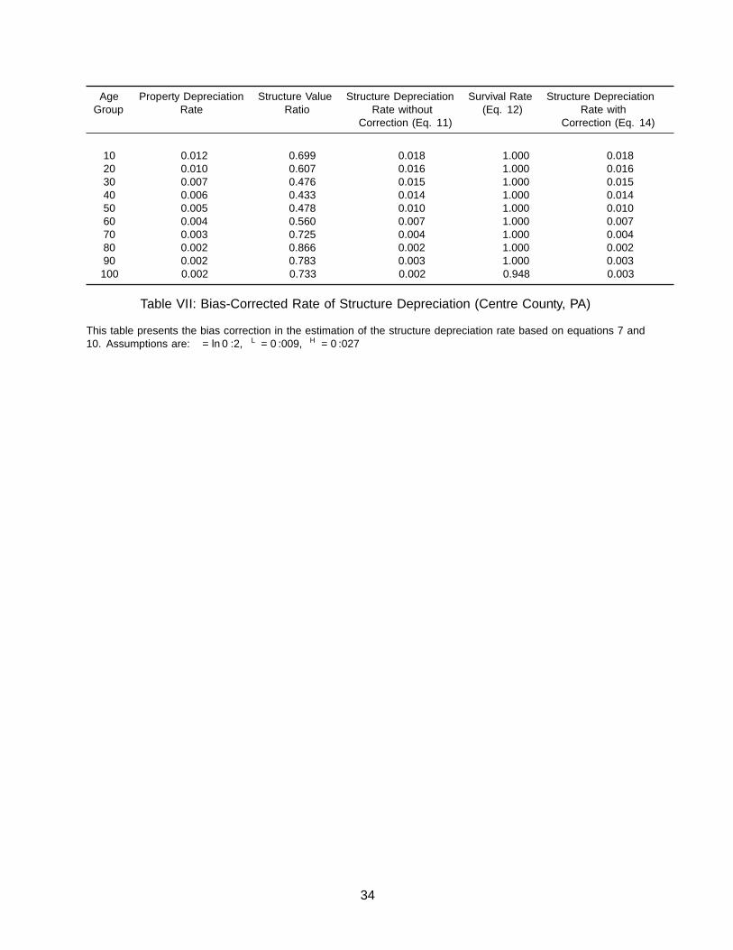
Age Property Depreciation Structure Value Structure Depreciation Survival Rate Structure DepreciationGroup Rate Ratio Rate without (Eq. 12) Rate with
Correction (Eq. 11) Correction (Eq. 14)
10 0.012 0.699 0.018 1.000 0.01820 0.010 0.607 0.016 1.000 0.01630 0.007 0.476 0.015 1.000 0.01540 0.006 0.433 0.014 1.000 0.01450 0.005 0.478 0.010 1.000 0.01060 0.004 0.560 0.007 1.000 0.00770 0.003 0.725 0.004 1.000 0.00480 0.002 0.866 0.002 1.000 0.00290 0.002 0.783 0.003 1.000 0.003100 0.002 0.733 0.002 0.948 0.003
Table VII: Bias-Corrected Rate of Structure Depreciation (Centre County, PA)
This table presents the bias correction in the estimation of the structure depreciation rate based on equations 7 and10. Assumptions are: ζ = ln 0.2, δL = 0.009, δH = 0.027
34
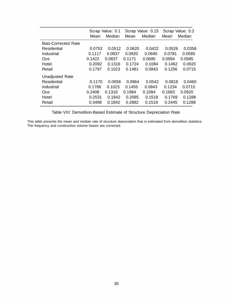
Scrap Value: 0.1 Scrap Value: 0.15 Scrap Value: 0.2Mean Median Mean Median Mean Median
Bias-Corrected RateResidential 0.0753 0.0512 0.0620 0.0422 0.0526 0.0358Industrial 0.1117 0.0837 0.0920 0.0690 0.0781 0.0585Office 0.1422 0.0837 0.1171 0.0690 0.0994 0.0585Hotel 0.2092 0.1316 0.1724 0.1084 0.1462 0.0920Retail 0.1797 0.1023 0.1481 0.0843 0.1256 0.0715
Unadjusted RateResidential 0.1170 0.0658 0.0964 0.0542 0.0818 0.0460Industrial 0.1766 0.1023 0.1455 0.0843 0.1234 0.0715Office 0.2408 0.1316 0.1984 0.1084 0.1683 0.0920Hotel 0.2531 0.1842 0.2085 0.1518 0.1769 0.1288Retail 0.3498 0.1842 0.2882 0.1518 0.2445 0.1288
Table VIII: Demolition-Based Estimate of Structure Depreciation Rate
This table presents the mean and median rate of structure depreciation that is estimated from demolition statistics.The frequency and construction volume biases are corrected.
35

0.2
.4.6
.81
0 10 20 30 40 50Building Age
Relative Price 95% CI
(a) Non-Parametric
-2.5
-2-1
.5-1
-.5
0M
arg
inal eff
ect
5 10 15 20 25 30 35 40 45 50Building age
Distance=140m (1 percentile) Distance=830m (median)Distance=3500m (99 percentile)
(b) Distance
-2.5
-2-1
.5-1
-.5
0M
arg
inal eff
ect
5 10 15 20 25 30 35 40 45Building age
Log floor=3.83 (1 percentile) Log floor=4.56 (median)Log floor=6.61 (99 percentile)
(c) Log Floor Area
-1.5
-1-.
50
.5M
arg
inal eff
ect
5 10 15 20 25 30 35 40 45 50Building age
Log lot=3.68 (1 percentile) Log lot=4.57 (median)Log lot=6.24 (99 percentile)
(d) Log Lot Area
Figure 1: Property Value Depreciation (Residential, Tokyo, Japan)
36

0.2
.4.6
.81
0 10 20 30 40 50Building Age
Relative Price 95% CI
(a) Non-Parametric
-1.5
-1-.
50
Marg
inal eff
ect
5 10 15 20 25 30 35 40 45 50Building age
Distance=170m (1 percentile) Distance=1300m (median)Distance=4800m (99 percentile)
(b) Distance
-2-1
.5-1
-.5
0M
arg
inal eff
ect
5 10 15 20 25 30 35 40 45Building age
Log floor=3.90 (1 percentile) Log floor=4.65 (median)Log floor=6.41 (99 percentile)
(c) Log Floor Area
-1.5
-1-.
50
Marg
inal eff
ect
5 10 15 20 25 30 35 40 45 50Building age
Log lot=3.82 (1 percentile) Log lot=5.00 (median)Log lot=6.68 (99 percentile)
(d) Log Lot Area
Figure 2: Property Value Depreciation (Residential, Outside Tokyo, Japan)
37

0.2
.4.6
.81
0 10 20 30 40 50Building Age
Relative Price 95% CI
(a) Non-Parametric-3
-2-1
01
5 10 15 20 25 30 35 40 45 50Building age
Distance=30m (1 percentile) Distance=320m (median)Distance=1950m (99 percentile)
(b) Distance
-2-1
.5-1
-.5
0.5
5 10 15 20 25 30 35 40 45 50Building age
Log floor=3.90 (1 percentile) Log floor=5.70 (median)Log floor=8.15 (99 percentile)
(c) Log Floor Area
-2-1
01
5 10 15 20 25 30 35 40 45 50Building age
Log lot=3.50 (1 percentile) Log floor=4.73 (median)Log floor=6.76 (99 percentile)
(d) Log Lot Area
Figure 3: Property Value Depreciation (Commercial, Tokyo, Japan)
38
0.2
.4.6
.81
0 10 20 30 40 50Building Age
Relative Price 95% CI
(a) Non-Parametric-2
-1.5
-1-.
50
5 10 15 20 25 30 35 40 45 50Building age
Distance=30m (1 percentile) Distance=500m (median)Distance=5200m (99 percentile)
(b) Distance
-1.5
-1-.
50
.5
5 10 15 20 25 30 35 40 45 50Building age
Log floor=3.95 (1 percentile) Log floor=5.70 (median)Log floor=8.30 (99 percentile)
(c) Log Floor Area
-1.5
-1-.
50
.5
5 10 15 20 25 30 35 40 45 50Building age
Log lot=3.56 (1 percentile) Log lot=5.11 (median)Log lot=7.64 (99 percentile)
(d) Log Lot Area
Figure 4: Property Value Depreciation (Commercial, Outside Tokyo, Japan)
39
0.2
.4.6
.81
0 10 20 30 40 50Building Age
Land StructureValue (new property = 1)
(a) Residential, Tokyo
0.2
.4.6
.81
0 10 20 30 40 50Building Age
Land StructureProperty Value (new property = 1)
(b) Residential, Outside Tokyo
0.2
.4.6
.81
0 10 20 30 40 50Building Age
Land StructureProperty Value (new property = 1)
(c) Commercial, Tokyo
0.2
.4.6
.81
0 10 20 30 40 50Building Age
Land StructureProperty Value (new property = 1)
(d) Commercial, Outside Tokyo
Figure 5: Decomposition of Property Value (Japan)
40
0.2
.4.6
.81
0 20 40 60 80 100Building Age
Relative Price 95% CI
(a) Non-Parametric-.
8-.
6-.
4-.
20
10 20 30 40 50 60 70 80 90 100Building age
distance=0.56 (1 percentile) distance=3.99 (median)distance=24.93 (99 percentile)
(b) Distance
-.6
-.4
-.2
0
10 20 30 40 50 60 70 80 90 100Building age
log floor=6.83 (1 percentile) log floor=7.55 (median)log floor=8.32 (99 percentile)
(c) Log Floor Area
-.6
-.4
-.2
0.2
10 20 30 40 50 60 70 80 90 100Building age
log lot=8.47 (1 percentile) log lot=9.60 (median)log lot=13.0 (99 percentile)
(d) Log Lot Area
Figure 6: Property Value Depreciation (Residential, Centre County, PA)
41
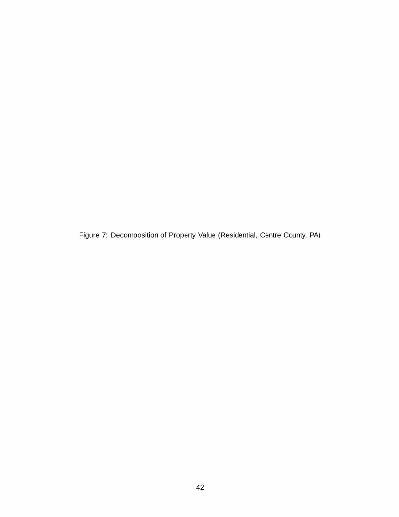
0.2
.4.6
.81
0 20 40 60 80 100Building Age
Land StructureProperty Value (new property = 1)
Figure 7: Decomposition of Property Value (Residential, Centre County, PA)
42

100,
000
200,
000
300,
000
400,
000
Valu
e (U
SD)
1,000 2,000 3,000 4,000Floor Area (sqft)
Fixed Characteristics Size-dependent Characteristics95% C.I.
(a) Foor Area and Property Value
010
020
030
040
0%
Incr
ease
in V
alue
0 200 400 600% Increase in Building Size
Fixed Characteristics Size-Dependent Characteristics45 degree line 95% C.I.
(b) Non-Marginal Change in Floor Area
.34
.46 .48 .5 .52 .53 .53 .55 .56
.3 .31 .32 .33 .33 .34 .35 .35 .36
0.2
.4.6
.81
Stru
ctur
e Va
lue
Shar
e
0 200 400 600% Increase in Building Size
Fixed Characteristics Size-Dependent Characteristics
(c) Structure Value Share
Figure 8: The Effct of Large Changes in Floor Area (Residential, Centre County, PA)
43
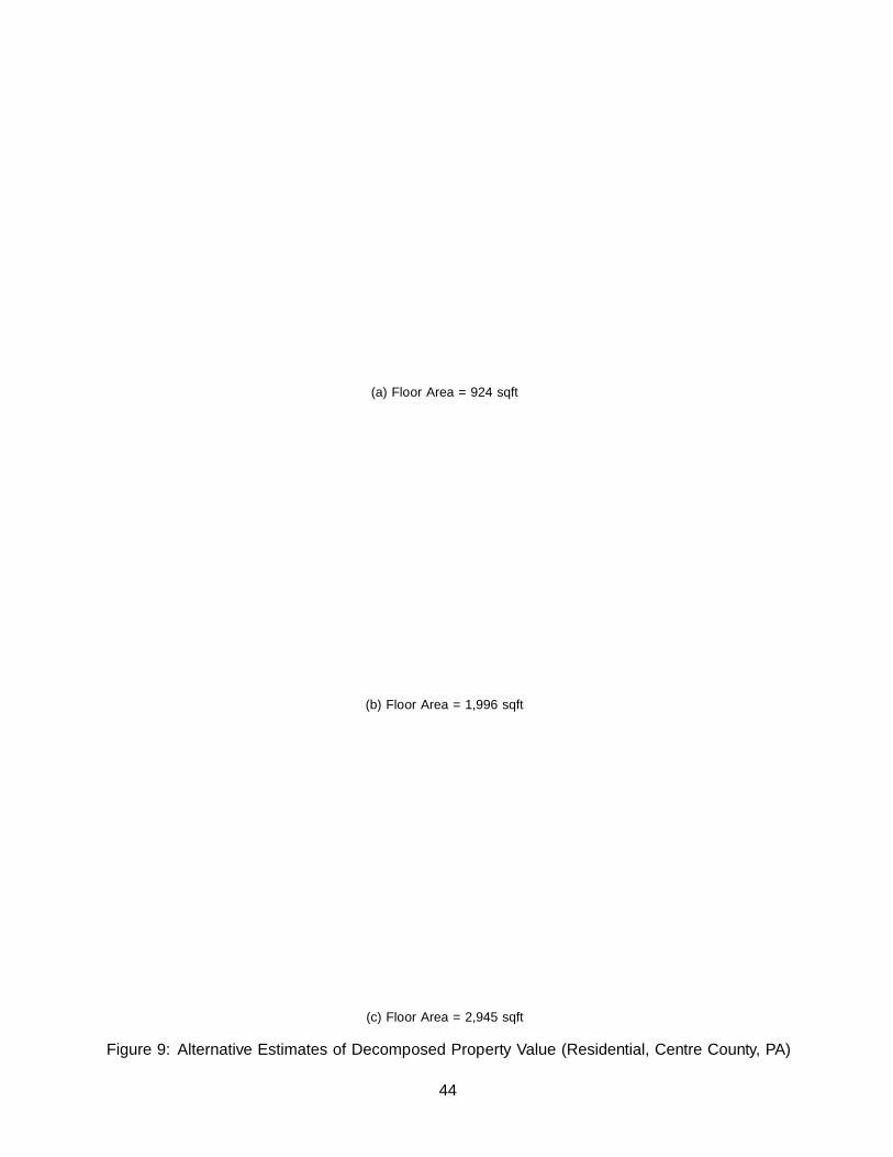
1.000.95 0.93
0.97 0.950.90
0.850.79
0.72 0.74 0.75
0.2
.4.6
.81
0 20 40 60 80 100Building Age
Land StructureProperty Value (new property = 1)
(a) Floor Area = 924 sqft
1.00
0.92
0.840.79
0.75 0.73 0.730.78 0.79 0.77 0.74
0.2
.4.6
.81
0 20 40 60 80 100Building Age
Land StructureProperty Value (new property = 1)
(b) Floor Area = 1,996 sqft
1.00
0.90
0.80
0.710.66 0.66 0.68
0.770.83
0.780.74
0.2
.4.6
.81
0 20 40 60 80 100Building Age
Land StructureProperty Value (new property = 1)
(c) Floor Area = 2,945 sqft
Figure 9: Alternative Estimates of Decomposed Property Value (Residential, Centre County, PA)
44

1.8% 1.6% 1.5% 1.4%1.0%
0.7%0.4% 0.2% 0.3% 0.3%
0%
2%
4%
6%
8%
10%
12%
14%
10 20 30 40 50 60 70 80 90 100
Age Group
Structure Depreciation Rate Property Depreciation Rate
(a) Centre County, Residential
5.8%
4.9%
5.6%5.2%
5.8%6.3% 6.5%
7.1%6.6%
7.7%
0%
2%
4%
6%
8%
10%
12%
14%
5 10 15 20 25 30 35 40 45 50
Age Group
Structure Depreciation Rate Property Depreciation Rate
(b) Tokyo, Residential
6.7%
5.4% 5.5%
6.1%
6.9% 7.1% 7.1%7.4% 7.5% 7.3%
0%
2%
4%
6%
8%
10%
12%
14%
5 10 15 20 25 30 35 40 45 50
Age Group
Structure Depreciation Rate Property Depreciation Rate
(c) Outside Tokyo, Residential
10.8%
12.9%
10.7%10.2% 10.1%
10.6% 10.5% 10.5%10.1% 10.0%
0%
2%
4%
6%
8%
10%
12%
14%
5 10 15 20 25 30 35 40 45 50
Age Group
Structure Depreciation Rate Property Depreciation Rate
(d) Tokyo, Commercial
9.8%
5.8%
8.6%8.9% 9.2% 9.4%
9.8%9.2% 9.3% 9.1%
0%
2%
4%
6%
8%
10%
12%
14%
5 10 15 20 25 30 35 40 45 50
Age Group
Structure Depreciation Rate Property Depreciation Rate
(e) Outside Tokyo, Commerical
Figure 10: Bias-Corrected Rates of Depreciation
This figure depicts the estimated annual property depreciation rate and the structure depreciation rate corrected for survivorshipbiases based on Tables VII and VI
45
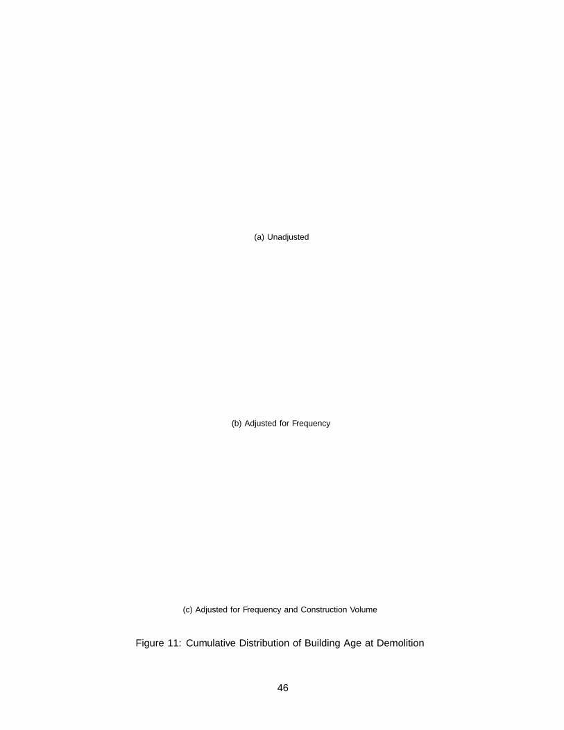
0.00
0.25
0.50
0.75
1.00
-3 years 3-5 years 5-10years
10-15years
15-20years
20-25years
25-30years
30-40years
40-50years
50 years-
Residential Industrial Office Hotel Commercial/Retail
(a) Unadjusted
0.00
0.25
0.50
0.75
1.00
-3 years 3-5 years 5-10years
10-15years
15-20years
20-25years
25-30years
30-40years
40-50years
50 years-
Residential Industrial Office Hotel Commercial/Retail
(b) Adjusted for Frequency
0.00
0.25
0.50
0.75
1.00
-3 years 3-5 years 5-10years
10-15years
15-20years
20-25years
25-30years
30-40years
40-50years
50 years-
Residential Industrial Office Hotel Commercial/Retail
(c) Adjusted for Frequency and Construction Volume
Figure 11: Cumulative Distribution of Building Age at Demolition
46

0.00
0.05
0.10
0.15
0.20
0.25
0.30
0.35
ResidentialIndustrialOfficeHotelCommercial/Retail
0.805 0.402 0.215 0.129 0.092 0.072 0.059 0.046 0.036 0.027
(a) Unadjusted
0.00
0.05
0.10
0.15
0.20
0.25
0.30
0.35
ResidentialIndustrialOfficeHotelCommercial/Retail
0.805 0.402 0.215 0.129 0.092 0.072 0.059 0.046 0.036 0.027
(b) Adjusted for Frequency
0.00
0.05
0.10
0.15
0.20
0.25
0.30
0.35
ResidentialIndustrialOfficeHotelCommercial/Retail
0.805 0.402 0.215 0.129 0.092 0.072 0.059 0.046 0.036 0.027
(c) Adjusted for Frequency and Construction Volume
Figure 12: Distribution of Depreciation Rates
47
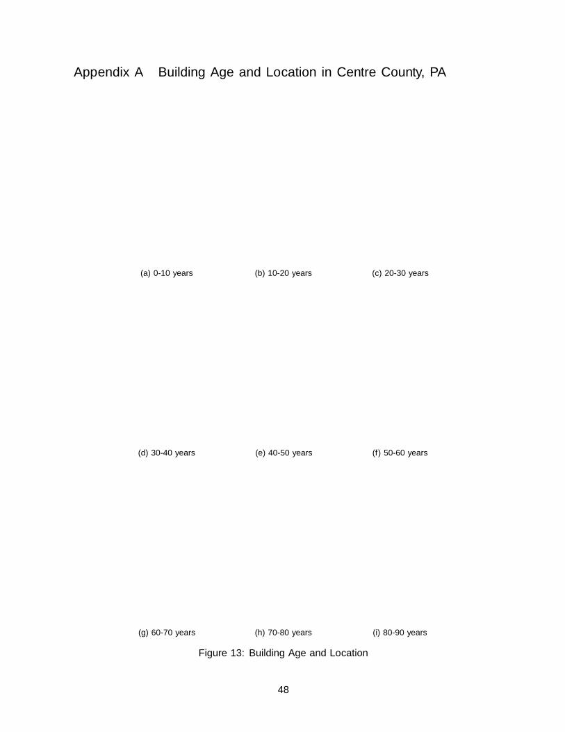
Appendix A Building Age and Location in Centre County, PA
(a) 0-10 years (b) 10-20 years (c) 20-30 years
(d) 30-40 years (e) 40-50 years (f) 50-60 years
(g) 60-70 years (h) 70-80 years (i) 80-90 years
Figure 13: Building Age and Location
48