†Department of Recreation, Sport and Tourism, University of Illinois, 104 Huff Hall,1206 South Fourth Street, Champaign, IL 61820, (217) 333-4410 (phone), (217) 244-1935 (fax),brh@uiuc.edu

††Department of Kinesiology and Community Health, University of Illinois,124B HuffHall MC588, 1206 South Fourth Street, Champaign, IL 61820 USA; Phone: 217-333-4242;Email:jruseski@uiuc.edu

Working Paper Series, Paper No. 06-13

Economic Determinants of Participation in Physical Activity and Sport

Brad R. Humphreys† and Jane E. Ruseski††

July 2006

AbstractThis paper examines the economic determinants of participation in physical activity by

developing and analyzing a consumer choice model of participation and by testing thepredictions of this model using data drawn from the Behavioral Risk Factor Surveillance Survey(BRFSS). Both emphasize that individuals face two distinct decisions: (1) should I participate insport?; and (2) how much time should I spend participating in sport? The evidence highlights theimportance of selectivity. The economic factors that affect these two decisions work in oppositedirections; factors that increase the likelihood of participation generally decrease the amount oftime spent participating.

JEL Classification Codes: I20, I12, I18, L83

Keywords: physical activity, time allocation, health production

* Previous drafts of this paper were presented at the IASE conference “New perspectives inSports Economics” in Bochum, Germany, May 2006 and the Western Economics AssociationAnnual meetings, in San Diego, CA, July 2006. We thank Chad Meyerhofer, Dennis Coates,Paul Downward, and Joe Riordan for their helpful comments on earlier drafts of this paper andChad Zanocco for his excellent research assistance.

Introduction

There is a growing perception among policymakers and public health researchers that individual’sdecisions about participating in physical activity, including sport, has an important economic com-ponent. Relatively little attention has been paid to this topic by economists. In this paper, wedevelop an economic model of the decision to participate in physical activity and test the predic-tions of this model using a nationally representative data set containing detailed information onparticipation in sport and other physical activities.

Much of this interest in the economic determinants of physical activity stems from the grow-ing literature on the economic causes and consequences of obesity. Poor nutrition and physicalinactivity are discretionary activities that can have a major impact on chronic diseases such asobesity (Cawley, 2004). Many plausible explanations for the rise in obesity have been advancedand a variety of policy interventions have been proposed to reduce the rate of obesity. However, theprevalence of meeting nutrition and and physical activity guidelines is low in the United States (Hillet al., 2004). Despite the important policy and public health aspects of participation in physicalactivity, little economic research has focused on the topic. There are a few notable exceptions tothis. One is the recent research by Cawley, et al. (2005) on physical education in the United States.Another is research on participation in physical activity from a leisure demand perspective; Davies(2002) is a recent example of research in this area. Still another is statistical analysis by Farrell andShields (2002) on the economic and demographic determinants of sporting participation in England.A final exception is the tangentially related research on the economic returns to participating inintercollegiate athletics in the United States spawned by interest in Title IX.

A possible explanation for the failure in meeting physical activity guidelines is a poor un-derstanding of the influence of economic factors on participation in physical activity and sport.Economics is useful for furthering our understanding because it provides a framework for study-ing how people allocate their time to competing activities and what economic, environmental anddemographic factors affect the decision to be physically active. Once the decision to participate ismade, the next decisions involve what activity, how often, how intense and how long. This paperbegins to bridge this gap in the literature by combining and adapting components of the SLOTH de-veloped by Cawley (2004) and commonly used recreation and leisure demand models to investigatethe economic determinants of participation in physical activity. The SLOTH framework is basedon Becker’s (1964) model of labor and leisure choice. This model assumes that individuals derivesatisfaction from the consumption of “basic commodities” like meals. These basic commodities areproduced by households using time and market commodities according to a production function.The consumption of basic goods has labor market implications because any time used to produceand enjoy basic commodities represents time spent not working. Participation in physical activityand sport is a basic commodity in this context.

The model developed in this paper incorporates the idea that individuals make two separatebut related decisions: (1) should I participate in sport?; and (2) how much time should I spendparticipating in sport? The model generates predictions about the relationship between physicalactivity, economic factors like income, and the opportunity cost of time. The model developedhere generates a number of predictions that provide new insight into the economic determinantsof participation in physical activity and sport. For example, the model predicts that the effect ofchanges in income on the decision to participate in physical activity and the effect on the amountof time spent in physical activity may have opposite signs. Participation in physical activity riseswith income, but time spent in physical activity declines with income. These predictions areempirically testable, and we find strong support for these predictions through the analysis of alarge, nationally representative data set containing a wealth of information about individual’s

2

participation in physical activity.

A Model of Participation in Physical Activity

Our model of participation in physical activity is an extension of the SLOTH framework of timeallocation. (Cawley 2004) The framework is based on Becker’s (1964) model of labor and leisurechoice. The basic idea is that people are involved in the production of their own health. Peoplecombine time with market goods to produce health. The SLOTH framework assumes that indi-viduals choose how to allocate their time to maximize their utility subject to budget, time andbiological constraints where SLOTH is an acronym for the activities to which individuals allocatetheir time. Specifically, S represents time spent sleeping; L represents time spent at leisure, Orepresents time spent at paid work; T represents time spent in transportation; and H representstime spent in home production, or unpaid work. Participation in physical activity and sport iscaptured in L, as is time spent in sedentary leisure activities such as watching television or playingcomputer games.

We combine the key temporal elements of the SLOTH framework with a recreation demandmodel (McConnell, 1992) to analyze both time allocation decisions and decisions about the purchaseof good and services related to active and passive leisure. The key behavioral decisions behind ourmodel are the separate but related decisions to participate in physical activity and how long toparticipate per episode of physical activity. We extend the SLOTH framework by recognizing thatsome of the activities in the SLOTH framework require time and goods and services purchasedin the marketplace. Suppose individuals choose how to allocate their time to various activitiesaccording to the following utility function:

max U(S, LF (TF , G), LU (TU , V ), O + T,C(TC , X)) (1)

where S is time spent sleeping; LF is a function describing leisure time devoted to physical activity;LU is a function describing leisure time devoted to sedentary activity; O + T is total time spentat work and getting to and from work; and C is a function describing time spent in householdproduction or unpaid work. The functions LF , LU and C have time arguments (TF , TU andTC) and market goods and services arguments (G, V and X). These functions recognize thatan individual’s decision to participate in physical activity requires not only time but also goodsand services purchased in the marketplace. Before introducing the time and budget constraints,we adapt components of the recreation demand model to reformulate and simplify the utilityfunction to emphasize the physical activity participation and duration decisions. Equation (1) canbe restated more compactly

max U(a, t, z) (2)

where a represents the individual’s decision to participate in physical activity; t is the amount oftime spent per episode of physical activity; and z represents the individual’s decision to engage inthe other activities in the SLOTH framework. z then is composite of S, O, T , C and LU ; a isequivalent to LF ; and t is equivalent to TF in the modified SLOTH framework.

Individuals choose how to best allocate their time and what bundle of goods and services topurchase subject to time and budget constraints. The budget constraint is

Y = Fa + caat + czz (3)

3

where Fa is the fixed cost of engaging in physical activity; ca is the variable cost associated withengaging in physical activity; and cz is the cost all other goods and services. The fixed costs ofphysical activity are one-time costs or flat recurring costs that individuals incur to participate inphysical activity but do not depend on how many times the individuals participates. An exampleof a fixed cost is the monthly membership dues at a health club. An individual pays this flat, fixedamount regardless of how many times he uses the gym during the month. Variable costs of physicalactivity are costs that do depend on the amount of time or the number of times the individualengages in physical activity. Examples of variable costs are equipment maintenance costs, coachesfees and personal trainer fees.

The time constraint is

T ∗ = at + θz (4)

where T ∗ is the time available for consumption activities such as physical activity and θ is timespent consuming z. Assume that T ∗, t and θ are measured in the same units such as hours. LetT be the total time available for work and all other activities. Hence, T ∗ = T − h where h is timespent working. If individuals can choose the amount of hours they work, then wage earnings w canbe expressed in terms of total time available and time spent not working

wh = w(T − at− θz). (5)

Equation (5) captures the notion that any time spent in physical activity and other activities is timenot available for work and reduces earnings. Thus, the wage is the opportunity cost of engaging inactivities other than work. The full budget (or income) constraint includes the opportunity cost oftime

y0 + w(T − T ∗) = Fa + paat + pzz (6)

where pa = ca +w and pz = cz +θw are the full costs of participating in physical activity and otheractivities.

Comparative Static Analysis

Consumers choose a, t and z to maximize utility subject to the full income constraint. The la-grangian for this problem is

V = U(a, t, z)− λ(Fa + pa · a · t + pzz − y) (7)

The first order conditions characterizing the optimal choices of a, t and z are found by partiallydifferentiating V with respect to the choice variables and the lagrange multiplier

∂V∂a = ∂U

∂a − λpat = 0∂V∂t = ∂U

∂t − λpat = 0∂V∂z = ∂U

∂z − λpz = 0∂V∂λ = −(Fa + pa · a · t + pzz − y) = 0.

We conduct a comparative static analysis of the consumer’s choice problem. We analyze the effectsof changes in income and the opportunity cost of time on the decisions to participate in physicalactivity and the amount of time spent participating in physical activity. In the comparative static

4

analysis we treat the decision to participate in physical activity as a continuous, but discrete countvariable rather than a dichotomous variable restricted to take on the values of zero or one. Thisapproach is consistent with the time dimension of the participation in physical activity data usedin our empirical analysis, the month prior to the survey. Each episode of physical activity requiresa separate participation decision, so the participation decision is made repeatedly over time. As aresult, observed episodes of physical activity are not limited to zero or one over the relevant timeperiod.

We first derive comparative static expressions for the the effect of a change in income (dy) onboth the participation decision a and the optimal amount of time spent in physical activity t. Thecomparative static expression for the effect of change in income (dy) on a holding dt, dpa, dpz anddFa constant and setting dt/dy = 0 is

∂a

∂y=

Uazpz − patUzz

pz(−Uaapz + Uzapat)− pat(−Uazpz + Uzzpat)(8)

The detailed derivation of the comparative static results are contained in the technical appendix.Convexity of the indifference curves requires the denominator of equation (8) to be positive and thesign depends on the sign of the numerator. Uzz < 0 by assumption, so the sign of the numeratordepends on the first term, which contains the term Uaz that cannot be signed a priori. If Uaz > 0,then ∂a

∂y > 0.Our intuition is that the cross-partial derivative, Uaz > 0, should be positive. This cross partial

describes the relationship between the marginal utility from participating in physical activity andthe marginal utility from other activities like meals or watching television. Participating in physicalactivity may lead to increased enjoyment of other non-active leisure activities. For example, if anindividual decides to go to the gym and work out, the marginal utility from a meal in a restaurantlater in the evening could be greater than the marginal utility received by a non-participant.

Next, we evaluate the comparative static derivative dt/dy to examine the effect of changes inincome on the optimal amount of time spent in physical activity by holding da, dpa, dpz and dFa

constant and setting da/dy = 0. We hold da constant because the decision about the amountof time an individual participates in physical activity is only relevant if the individual chooses toparticipate. The comparative static expression is

∂t

∂y=

Utzpz − paaUzz

pz(−Uttpz + Uztpaa)− paa(−Utzpz + Uzzpaa)(9)

Again, convexity of the indifference curves requires the denominator of equation (9) to be positiveand the sign depends on the sign of the numerator. Uzz < 0 by assumption, so the sign of thenumerator depends on the first term in the numerator, which contains the term Utz that cannotbe signed a priori. If Utz < 0, then ∂t

∂y < 0. This cross-partial is difficult to sign and we have nointuition about what this sign might be. However, we empirically estimate the effect of changes inincome on the amount of time spent in physical activity below. This estimate will shed light onthe sign of this term, and the nature of the relationship between utility derived from time spent inphysical activity and utility derived from consuming other goods and spending time in other leisureactivities.

The opportunity cost of time affects the decision to participate in physical activity and theamount of time devoted to physical activity. Recall, pa = ca+w and pz = cz +θw. The opportunitycost of time is the wage rate w. Expanding the lagrangian to explicitly show the full cost of timespent in physical activity and all other activities is

V = U(a, t, z)− λ(Fa + (ca + w) · a · t + (cz + θw)z − y). (10)

5

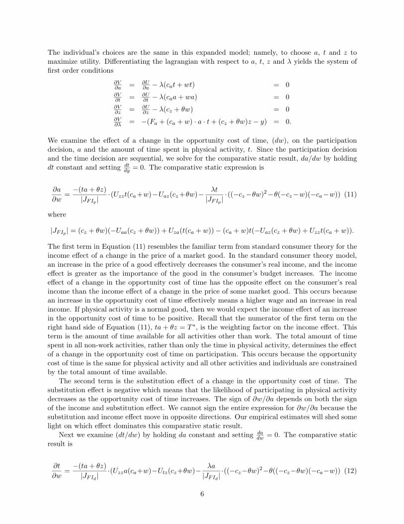
The individual’s choices are the same in this expanded model; namely, to choose a, t and z tomaximize utility. Differentiating the lagrangian with respect to a, t, z and λ yields the system offirst order conditions

∂V∂a = ∂U

∂a − λ(cat + wt) = 0∂V∂t = ∂U

∂t − λ(caa + wa) = 0∂V∂z = ∂U

∂z − λ(cz + θw) = 0∂V∂λ = −(Fa + (ca + w) · a · t + (cz + θw)z − y) = 0.

We examine the effect of a change in the opportunity cost of time, (dw), on the participationdecision, a and the amount of time spent in physical activity, t. Since the participation decisionand the time decision are sequential, we solve for the comparative static result, da/dw by holdingdt constant and setting dt

dy = 0. The comparative static expression is

∂a

∂w=

−(ta + θz)|JFIp |

·(Uzzt(ca +w)−Uaz(cz +θw)− λt

|JFIp |·((−cz−θw)2−θ(−cz−w)(−ca−w)) (11)

where

|JFIp | = (cz + θw)(−Uaa(cz + θw)) + Uza(t(ca + w))− (ca + w)t(−Uaz(cz + θw) + Uzzt(ca + w)).

The first term in Equation (11) resembles the familiar term from standard consumer theory for theincome effect of a change in the price of a market good. In the standard consumer theory model,an increase in the price of a good effectively decreases the consumer’s real income, and the incomeeffect is greater as the importance of the good in the consumer’s budget increases. The incomeeffect of a change in the opportunity cost of time has the opposite effect on the consumer’s realincome than the income effect of a change in the price of some market good. This occurs becausean increase in the opportunity cost of time effectively means a higher wage and an increase in realincome. If physical activity is a normal good, then we would expect the income effect of an increasein the opportunity cost of time to be positive. Recall that the numerator of the first term on theright hand side of Equation (11), ta + θz = T ∗, is the weighting factor on the income effect. Thisterm is the amount of time available for all activities other than work. The total amount of timespent in all non-work activities, rather than only the time in physical activity, determines the effectof a change in the opportunity cost of time on participation. This occurs because the opportunitycost of time is the same for physical activity and all other activities and individuals are constrainedby the total amount of time available.

The second term is the substitution effect of a change in the opportunity cost of time. Thesubstitution effect is negative which means that the likelihood of participating in physical activitydecreases as the opportunity cost of time increases. The sign of ∂w/∂a depends on both the signof the income and substitution effect. We cannot sign the entire expression for ∂w/∂a because thesubstitution and income effect move in opposite directions. Our empirical estimates will shed somelight on which effect dominates this comparative static result.

Next we examine (dt/dw) by holding da constant and setting dadw = 0. The comparative static

result is

∂t

∂w=

−(ta + θz)|JFId

|·(Uzza(ca+w)−Utz(cz+θw)− λa

|JFId|·((−cz−θw)2−θ((−cz−θw)(−ca−w)) (12)

6

where

|JFId| = (cz + θw)(−Utt(cz + θw)) + Utz(a(ca + w))− (ca + w)a(−Utz(cz + θw) + Uzza(ca + w)).

The interpretation of this comparative static result is the same as the interpretation of Equation(11). The first term is the income effect and the second term is the substitution effect. Again, thisterm cannot be signed a priori because of the opposing signs of the income and substitution effects.We empirically estimate the effect of changes in the opportunity cost of time on the amount of timespent in physical activity below.

In summary, the model developed in this section describes consumer’s decisions about partici-pating in physical activities, time spent participating in physical activities, time spent in non-activeleisure activities, the purchase of other goods, services, and the time spent consuming these othergoods and services. We conduct a comparative statics analysis to examine the effect of changes inincome and the opportunity cost of time on participation and time spent in physical activity. Toour knowledge, no previous research has developed and solved a formal consumer choice model ofphysical activity participation and time decisions.

Because of the lack of research in this area, a formal empirical test of some of the predictionsof this model is an important step in research into the economic determinants of physical activity.In the following section we describe a large, nationally representative data set that contains a richamount of data on participation in physical activity and other economic and demographic factors.We then use these data to test the economic predictions that emerge from the consumer choicemodel and estimate the effect of social and behavioral factors on physical activity.

Data Description and Sample Statistics

Since little previous research has focused on the economic determinants of participation in sport andphysical activity, we empirically test the predictions of our consumer choice model in order to assesstheir validity. We use data from the Behavioral Risk Factor Surveillance System (BRFSS). Thesurvey is conducted annually by telephone to a random representative sample of the population overthe age of 18 in each U.S. state by the Center for Disease Control and Prevention in conjunctionwith U.S. states. The survey collects uniform state-specific data on preventative health factors,behavioral risk factors, and other economic and demographic characteristics and includes a rotatingselection of modules one of which is on exercise and physical activity.

The BRFSS physical activity data is a rich source of information on participation in physicalactivities in the United States and has been used in some previous economic research. For example,Chou, et al. (2002a,2002b) used this data set to examine the link between obesity and physicalactivity. The survey asks about both frequency and duration of participation, which providesa relatively complete picture of self reported physical activities. The survey also asks questionsabout demographic factors like age, gender, race, ethnicity, and marital status, and questionsabout economic factors like income and labor market participation. This makes the BRFSS dataan ideal setting for examining the economic determinants of physical activity. The physical activitymodule is not included in every year. We use data from the 2000 BRFSS survey, which included amodule about physical activity and exercise.

184,450 persons were surveyed in the 2000 BRFSS survey. The 2000 survey included residents ofPuerto Rico, and the exercise module was not administered to residents of Illinois that year. Afterexcluding these observations, and some observations for individuals with a reported age under 18,a sample of 175,246 individuals remained. Table 1 shows some basic summary statistics for thissample of 175,246 individuals.

7

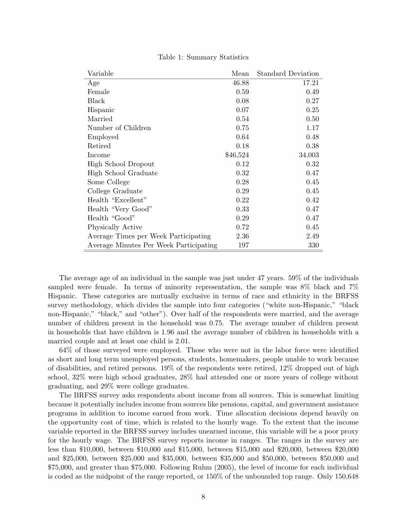
Table 1: Summary Statistics

Variable Mean Standard DeviationAge 46.88 17.21Female 0.59 0.49Black 0.08 0.27Hispanic 0.07 0.25Married 0.54 0.50Number of Children 0.75 1.17Employed 0.64 0.48Retired 0.18 0.38Income $46,524 34,003High School Dropout 0.12 0.32High School Graduate 0.32 0.47Some College 0.28 0.45College Graduate 0.29 0.45Health “Excellent” 0.22 0.42Health “Very Good” 0.33 0.47Health “Good” 0.29 0.47Physically Active 0.72 0.45Average Times per Week Participating 2.36 2.49Average Minutes Per Week Participating 197 330

The average age of an individual in the sample was just under 47 years. 59% of the individualssampled were female. In terms of minority representation, the sample was 8% black and 7%Hispanic. These categories are mutually exclusive in terms of race and ethnicity in the BRFSSsurvey methodology, which divides the sample into four categories (“white non-Hispanic,” “blacknon-Hispanic,” “black,” and “other”). Over half of the respondents were married, and the averagenumber of children present in the household was 0.75. The average number of children presentin households that have children is 1.96 and the average number of children in households with amarried couple and at least one child is 2.01.

64% of those surveyed were employed. Those who were not in the labor force were identifiedas short and long term unemployed persons, students, homemakers, people unable to work becauseof disabilities, and retired persons. 19% of the respondents were retired, 12% dropped out of highschool, 32% were high school graduates, 28% had attended one or more years of college withoutgraduating, and 29% were college graduates.

The BRFSS survey asks respondents about income from all sources. This is somewhat limitingbecause it potentially includes income from sources like pensions, capital, and government assistanceprograms in addition to income earned from work. Time allocation decisions depend heavily onthe opportunity cost of time, which is related to the hourly wage. To the extent that the incomevariable reported in the BRFSS survey includes unearned income, this variable will be a poor proxyfor the hourly wage. The BRFSS survey reports income in ranges. The ranges in the survey areless than $10,000, between $10,000 and $15,000, between $15,000 and $20,000, between $20,000and $25,000, between $25,000 and $35,000, between $35,000 and $50,000, between $50,000 and$75,000, and greater than $75,000. Following Ruhm (2005), the level of income for each individualis coded as the midpoint of the range reported, or 150% of the unbounded top range. Only 150,648

8

people responded to the income question in the 2000 BRFSS survey. This sub-sample forms thebasis for the empirical work in the following sections. From Table 1, the average level of income inthe sample was $46,524.

Physical Activity Measures

The 2000 BRFSS survey contained a module of questions on physical activity. These questionswere asked to the entire sample except residents of Illinois. The basic physical activity question inthe BRFSS survey is

During the past month, did you participate in any physical activities or exercises suchas running, calisthenics, golf, gardening, or walking for exercise?

We initially define participation in physical activity using this survey question. From Table 1, 72%of the sample answered yes to this question. This is a relatively high participation rate for physicalactivity, but the question is not qualified by any statement about the duration of the activity,and many people may answer yes even when they spend very little time participating in physicalactivity. Fortunately, BRFSS contains more detailed questions about physical activity and exercisethan a simple participation question. The survey also elicits detailed information about the type ofactivity, the frequency of participation, and the duration of participation in physical activity. Thefirst question that elicits additional detail about the type of physical activity undertaken is

What type of physical activity or exercise did you spend the most time doing during thepast month?

The responses to this question were a long list of activities from running to raking the lawn. Table2 contains the entire list of physical activities reported and their frequency in the sample. Theresponses on Table 2 show a wide variation in reported physical activities in the sample. Theactivities also differ in a number of important ways. They require different amounts of travel,equipment, time and effort on the part of the participant. Some, like walking or running, can bedone alone while others, like soccer or volleyball, require additional participants; still others can bedone alone or in groups. Because of the heterogeneity of the activities, future research will considergrouping the activities by common characteristics like equipment required, level of exertion, caloriesburned and other identifiable factors.

Walking is by far the most common physical activity. Just over 50% of the sample, 65,620individuals, reported walking as their primary or secondary type of physical activity over the pastmonth. No other type of physical activity was even close. The high reported frequency of walkingas the primary form of physical activity in the sample probably reflects the relatively low costof this activity. Unlike many of the other activities listed on Table 2, walking does not requireany specialized equipment or facilities. It can be done in almost any setting under almost anyconditions.

The survey asks about a first and a second activity participated in over the last month. 31% ofthose surveyed reported participating in two activities over the previous month. In this paper, wesimply add up time spent in the primary and secondary physical activity to get a total measure oftime spent in physical activity per week.

BRFSS also contains detailed information about how frequently individuals in the survey par-ticipated in physical activities in the past month, and how much time the individuals spent in eachactivity on average. These data provide enough detail to construct an estimate of the number oftimes per week and minutes per week that each individual in the survey spent participating in some

9

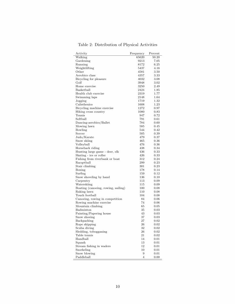
Table 2: Distribution of Physical Activities

Activity Frequency PercentWalking 65620 50.20Gardening 9213 7.05Running 8172 6.25Weightlifting 5437 4.16Other 4581 3.50Aerobics class 4357 3.33Bicycling for pleasure 4032 3.08Golf 3948 3.02Home exercise 3250 2.49Basketball 2424 1.85Health club exercise 2319 1.77Swimming laps 2148 1.64Jogging 1719 1.32Calisthenics 1608 1.23Bicycling machine exercise 1272 0.97Hiking cross country 1080 0.83Tennis 947 0.72Softball 791 0.61Dancing-aerobics/Ballet 784 0.60Mowing lawn 585 0.45Bowling 544 0.42Soccer 505 0.39Judo/Karate 479 0.37Snow skiing 465 0.36Volleyball 476 0.36Horseback riding 438 0.34Hunting large game - deer, elk 436 0.33Skating - ice or roller 426 0.33Fishing from riverbank or boat 312 0.24Racqetball 299 0.23Stair climbing 301 0.23Boxing 178 0.14Surfing 159 0.12Snow shoveling by hand 136 0.10Carpentry 113 0.09Waterskiing 115 0.09Boating (canoeing, rowing, sailing) 100 0.08Raking lawn 110 0.08Touch football 104 0.08Canoeing, rowing in competition 84 0.06Rowing machine exercise 74 0.06Mountain climbing 65 0.05Badminton 35 0.03Painting/Papering house 43 0.03Snow shoeing 37 0.03Backpacking 27 0.02Rope skipping 26 0.02Scuba diving 32 0.02Sledding, tobogganing 26 0.02Table tennis 21 0.02Handball 14 0.01Squash 13 0.01Stream fishing in waders 12 0.01Snorkeling 10 0.01Snow blowing 9 0.01Paddleball 4 0.00

10

physical activity. In estimating the duration of participation, we included the reported amount oftime spent in both the primary and secondary physical activity.

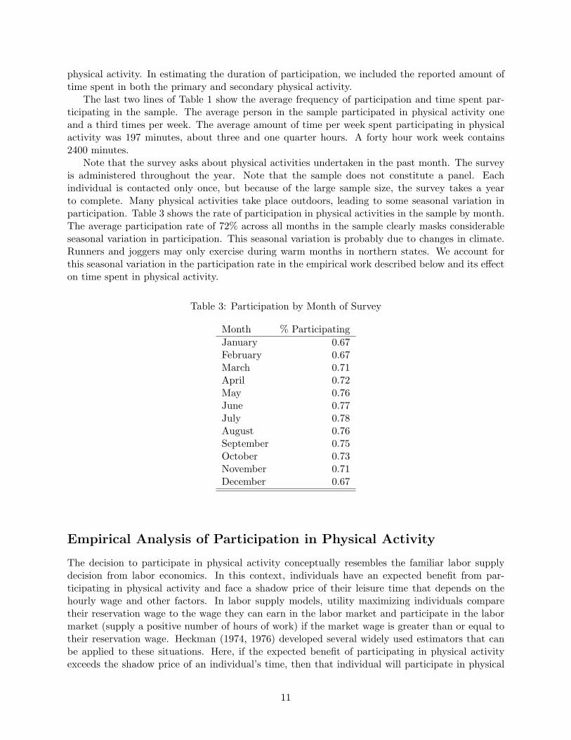
The last two lines of Table 1 show the average frequency of participation and time spent par-ticipating in the sample. The average person in the sample participated in physical activity oneand a third times per week. The average amount of time per week spent participating in physicalactivity was 197 minutes, about three and one quarter hours. A forty hour work week contains2400 minutes.

Note that the survey asks about physical activities undertaken in the past month. The surveyis administered throughout the year. Note that the sample does not constitute a panel. Eachindividual is contacted only once, but because of the large sample size, the survey takes a yearto complete. Many physical activities take place outdoors, leading to some seasonal variation inparticipation. Table 3 shows the rate of participation in physical activities in the sample by month.The average participation rate of 72% across all months in the sample clearly masks considerableseasonal variation in participation. This seasonal variation is probably due to changes in climate.Runners and joggers may only exercise during warm months in northern states. We account forthis seasonal variation in the participation rate in the empirical work described below and its effecton time spent in physical activity.

Table 3: Participation by Month of Survey

Month % ParticipatingJanuary 0.67February 0.67March 0.71April 0.72May 0.76June 0.77July 0.78August 0.76September 0.75October 0.73November 0.71December 0.67

Empirical Analysis of Participation in Physical Activity

The decision to participate in physical activity conceptually resembles the familiar labor supplydecision from labor economics. In this context, individuals have an expected benefit from par-ticipating in physical activity and face a shadow price of their leisure time that depends on thehourly wage and other factors. In labor supply models, utility maximizing individuals comparetheir reservation wage to the wage they can earn in the labor market and participate in the labormarket (supply a positive number of hours of work) if the market wage is greater than or equal totheir reservation wage. Heckman (1974, 1976) developed several widely used estimators that canbe applied to these situations. Here, if the expected benefit of participating in physical activityexceeds the shadow price of an individual’s time, then that individual will participate in physical

11

activity.Let Ai be the amount of time that individual i spends in some physical activity, Xi be a vector

of variables, including characteristics of individual i that might explain the time that individual ispends in physical activity and β be a vector of unobservable parameters. The data set used herecontains both individuals who participate in physical activity (i = 1, 2, . . . N1 where Ai > 0) andindividuals that do not participate in physical activity (i = N1 + 1, N1 + 2, . . . , N , where Ai = 0).The set of individuals who participate in physical activity will be referred to as S1 and the set ofindividuals who do not participate will be referred to as S2.

Given the available data, it would be possible to estimate an equation explaining observed timespent in physical activity

Ai = βXi + ei (13)

where ei is an unobservable mean zero, constant variance random variable capturing factors otherthan Xi that affect individual is decision to participate in physical activity. However, if the timespent in physical activity by non-participants is set to zero and the parameters of equation (13)estimated using the Ordinary Least Squares (OLS) estimator, the parameter estimates will beinconsistent because the model incorrectly assumes that equation (13) can be applied to all indi-viduals in the sample. This is the well-known selectivity problem in econometrics. Heckman (1974,1976) developed a two-step procedure to deal with selectivity of this type. The Heckman selectivitycorrection is based on a reduced form approach to individual’s participation decision.

Note that if all individuals in the sample participated in physical activity, then the expectedvalue of the time spent in physical activity would be

E[Ai] = βXi

but when Ai = 0 for some individuals the expected value of the time spent in physical activity is

E[Ai] = Prob(Ai > 0) · E[Ai|Ai > 0] + Prob(Ai ≤ 0) · 0.

Applying Heckman’s approach implies that individuals make two choices related to physicalactivity: a choice to participate in physical activity (the participation decision) and a choice abouthow much time to spend in physical activity conditional on the decision to participate (the timedecision). To implement Heckman’s approach, partition Xi into two sets of variables (Xi1, Xi2)where Xi1 affects the participation decision and Xi2 affects the time decision.

Given this partitioning of Xi, the time decision can be expressed

Ai = β1Xi1 + ui if Ai = β1Xi1 + ui > 0

and otherwise

Ai = 0.

The participation decision is modeled as a function of observable factors (Xi2), an unobservablemean zero, constant variance random error term (νi), and some unobservable factor wi∗ thatcaptures the benefit that the individual gets from participating in physical activity. Let σν be thevariance of ν. If w∗

i > 0 then the individual participates in physical activity but if wi∗ ≤ 0 thenthe individual does not participate. Formally

Ai > 0 if w∗i > 0

Ai = 0 if w∗i ≤ 0

12

and w∗i is determined by

w∗i = β2Xi2 + νi.

The covariance between νi and ui is σuν . This can be shown to equal σνσuρ where ρ the coefficientof correlation between the two error terms.

This model for the determination of w∗i implies a selection rule based on the sign of this unob-

servable variable

Ai > 0 if νi > −β2Xi2

Ai = 0 if νi ≤ −β2Xi2.

This selection rule simply indicates that an individual compares the benefit of participating inphysical activity, reflected by the realization of νi to the cost of participating in the activity,represented by β2Xi2. If the benefit exceeds the cost, then w∗

i is positive and the individualparticipates. If the cost exceeds the benefit, then w∗

i is negative and the individual does notparticipate. Based on this selection rule, the expected value of Ai is

E[Ai] = Φ(

β2Xi2

σν

)· E[Ai|νi > −β2Xi2] +

[1− Φ

(β2Xi2

σν

)]where Φ(·) is the standard normal distribution function. Also note that

E[Ai|νi > −β2Xi2] = β1Xi1 + E[ui|νi > −β2Xi2]= β1Xi1 + σuν

σν

= β1Xi1 + ρσuh(

β2Xi2σν

).

The Heckman two step procedure is a sequential procedure:

1. Estimate β2/σν using the probit estimator. This involves maximizing the likelihood function

` =∏i∈S2

[1− Φ

(β2Xi2

σν

)]·

∏i∈S1

Φ(

β2Xi2

σν

)(14)

with respect to β2/σν .

2. Use the estimate of β2/σν to estimate h(·) and add this variable to the time equation. Theexpanded time equation

Ai = β1Xi1 +σuν

σνh

(β2Xi2

σν

)+ ui (15)

is estimated using OLS.

The OLS estimator generates unbiased and consistent estimates of the parameters of equation(15) because of the correction for selectivity captured by equation (14). For the Heckman proce-dure to work, Xi2 must contain some variables not in Xi1, and these variables must identify theparticipation decision.

13

Results and Discussion

Again, the process of participating in physical activity clearly includes selectivity. Individualsare deciding to either participate in a physical activity or not participate, and after making theparticipation decision they determine how long to participate. We use the two step Heckmanprocedure to account for selectivity in the behavior of the survey participants. The first stage ofthe Heckman procedure analyzes the participation decision. This involves estimating a model witha discrete dependent variable that is equal to one if the individual participates in some physicalactivity and is equal to zero if the individual does not participate. The vector of explanatoryvariables must contain some variables that do not enter the time equation in order to identify theparticipation decision. Ideally, these variables should explain some of the observed participationbehavior.

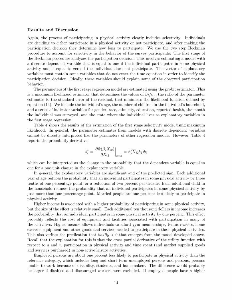
The parameters of the first stage regression model are estimated using the probit estimator. Thisis a maximum likelihood estimator that determines the values of β2/σν , the ratio of the parameterestimates to the standard error of the residual, that minimizes the likelihood function defined byequation (14). We include the individual’s age, the number of children in the indivdual’s household,and a series of indicator variables for gender, race, ethnicity, education, reported health, the monththe individual was surveyed, and the state where the individual lives as explanatory variables inthe first stage regression.

Table 4 shows the results of the estimation of the first stage selectivity model using maximumlikelihood. In general, the parameter estimates from models with discrete dependent variablescannot be directly interpreted like the parameters of other regression models. However, Table 4reports the probability derivative

b∗i =∂Φ(β2Xi2)

∂Xi2

∣∣∣∣x=x

= φ(Xi2b2)bi

which can be interpreted as the change in the probability that the dependent variable is equal toone for a one unit change in the explanatory variable.

In general, the explanatory variables are significant and of the predicted sign. Each additionalyear of age reduces the probability that an individual participates in some physical activity by threetenths of one percentage point, or a reduction of two percent per decade. Each additional child inthe household reduces the probability that an individual participates in some physical activity byjust more than one percentage point. Married people are one per cent less likely to participate inphysical activity.

Higher income is associated with a higher probability of participating in some physical activity,but the size of the effect is relatively small. Each additional ten thousand dollars in income increasesthe probability that an individual participates in some physical activity by one percent. This effectprobably reflects the cost of equipment and facilities associated with participation in many ofthe activities. Higher income allows individuals to afford gym memberships, tennis rackets, homeexercise equipment and other goods and services needed to participate in these physical activities.This also verifies the predication that ∂a/∂y > 0 that emerges from the model developed above.Recall that the explanation for this is that the cross partial derivative of the utility function withrespect to a and z, participation in physical activity and time spent (and market supplied goodsand services purchased) in non-active leisure activities.

Employed persons are about one percent less likely to participate in physical activity than thereference category, which includes long and short term unemployed persons and persons, personsunable to work because of disability, students, and homemakers. The difference would probablybe larger if disabled and discouraged workers were excluded. If employed people have a higher

14

Table 4: Participation Equation Estimation Results

Variable Probability Derivative P-valueAge -0.003 0.000Married -0.013 0.000Number of Children -0.011 0.000Income (thousands) 0.001 0.000Employed -0.008 0.013Retired 0.076 0.000High School Graduate 0.054 0.000Some College 0.107 0.000College Graduate 0.156 0.000Female -0.021 0.000Black -0.043 0.000Hispanic -0.059 0.000Reported Health Excellent 0.163 0.000Reported Health Very Good 0.141 0.000Reported Health Good 0.081 0.000January -0.108 0.000February -0.121 0.000March -0.067 0.000April -0.047 0.010May -0.014 0.018July -0.007 0.260August -0.009 0.125September -0.028 0.001October -0.047 0.000November -0.076 0.000December -0.116 0.000Observations 150,648Pseudo R2 0.091

15

opportunity cost of time than the unemployed, home makers, and students, then the sign of thisparameter suggests that the unsigned cross partial derivative from the model, Utz is negative.

The dummy variables for educational attainment exhibit an interesting pattern. The probabilityof participation increases with the level of education. The omitted category is people who did notcomplete high school. High school graduates are less likely to participate in physical activities thanhigh school dropouts, those who attended some college are more likely to participate than highschool graduates, and college graduates are more likely to participate than those with some college.This pattern could be due to occupational sorting of individuals with different levels of education.For example, if high school dropouts tend to work part time or seasonally, they might have morefree time to participate in physical activities than high school graduates, if high school graduatestend to work full time. Alternatively, Grossman’s (1972) model of health production predicts thatindividuals with more education are more efficient in producing health. If participation in physicalactivity leads to improved health, then the estimated parameters on the education variables could bepart of the mechanism through which individuals produce better health, supporting the predictionsof Grossman’s model.

After controlling for differences in income and the presence of children, females are two per-cent less likely to participate in some physical activity than males. This probably reflects greaterresponsibility in childcare and home production activities. Blacks and Hispanics are less likely toparticipate in some physical activity than whites. Many of these differences may simply reflect thatemployed minorities have poor access to the goods and services needed to participate in physicalthan whites.

The reported health of individuals has a significant impact on participation in physical activ-ity. The reference group is individuals who reported their general health as “fair” or poor. It isimportant to remember that this estimated is conditional on the effect of age on participation insome physical activity. Individuals in poor health would be expected to walk less, or perform anyphysical activity. Also, since the participation decision is estimated using maximum likelihood, anycorrelation between reported health and the true health of the individual, which will be captured bythe equation error term in the participation decision model, will not lead to econometric problems.

The month indicator variables are also highly significant and follow a logical pattern. Recall thatthe survey asks about participation in a physical activity in the previous month, and individualsare surveyed throughout the calendar year. Many physical activities take place outside, and afair number may have strong seasonal participation components, like gardening. The patternon the month dummy variables shows that individuals in the sample were more likely to reportparticipation in a physical activity in the summer and less likely to report participation in the winter.Again, note that the data do not constitute a panel. This seasonal variation in participation is isacross different individuals in the sample.

The model included a set of dummy variables indicating the state in which individuals lived.These state effects might capture the quantity and distance of recreation areas and sports facilities,climate, and variation in travel costs due to transportation infrastructure and traffic congestion.The estimates on these variables are not reported, but many of them were significant and the signswere both positive and negative. These state indicator variables may capture a variety of underlyingfactors related to climate, geography, population density, patterns of urbanization, transportationnetworks, and the supply of goods and services related to physical activity like playing fields,sporting goods stores, and health clubs across states. The significance of the state of the stateindicators suggests that future research should focus on collecting additional state-specific datato quantify these factors, in order to better identify specific factors that affect participation inphysical activity. Overall, the model explains just under six percent of the observed variation inparticipation.

16

Table 5: Time Equation Estimation Results

ParameterVariable Estimate P-valueAge 0.908 0.000Married -18 0.000Income (thousands) -0.270 0.000Employed 31 0.000Retired -0.178 0.947High School Graduate -37 0.000Some College -67 0.000College Graduate -104 0.000Female -75 0.000Black 15 0.003Hispanic 26 0.000Constant 519 0.000λ -324 0.000Wald χ2 8539 0.000

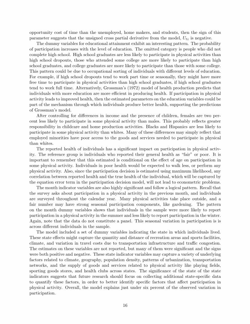
In the second stage, the time equation, equation (15) is estimated using OLS. Table 5 containsthe parameter estimates and P-values from estimating equation (15) with OLS. The vector of monthindicator variables was also included in the time equation, but the estimated parameters on thesevariables are not reported. Most were significant, and indicated that time spent in physical activitywas higher in the summer and lower in other months. This regression model explains variationin the amount of time individuals spend participating in physical activity. The second term onthe right hand side of equation (15) is calculated from the first stage regression, and is sometimesreferred to as the “inverse Mills ratio” in the literature. The parameter on this variable indicates thecorrelation between the error term on the selectivity equation and the time equation, and includingthis term ensures that the other parameter estimates do not reflect selectivity bias.

The identifying variables in the first stage regression are the number of children present in thehousehold, the three variables indicating reported health status, and the vector of dummy variablesindicating state of residence. The parameter estimates for the time equation were not sensitive toincluding the reported health status variables and the state of residence indicators in the secondstage.

The estimates of the time equation reveal several interesting features. First, after correctingfor selectivity, the sign on the age parameter is positive so individuals who choose to participatein physical activity tend to increase the time spent as age increases, other things constant. Theincrease in time spent in physical activity is about one minute per year. Married people spendabout 18 minutes less per week participating in physical activities than single people.

The parameters on the race, gender and ethnicity show interesting patterns. Although blacksand Hispanics are less likely to participate in physical activity, those who do choose to participatespend more time in physical activity than whites. One implication of this result is that interventionsaimed at increasing the participation of these groups might be very effective, in that the individualsinduced to switch from non-participation to participation would spend a significant amount of timeengaging in physical activity.

Females spend less time in physical activities than males. This difference could be due to

17

occupational choices, if females tend to sort themselves into occupations that require more hours ofwork, or offer less job flexibility than males. Examples of such occupations include nursing, primaryand secondary education, and secretarial work. If could also reflect differences in the underlyingtypes of physical activities preferred by males and females.

Education has a negative effect on the amount of time individuals spend participating in physicalactivity, and the decrease in time spent in physical activity increases with the level of education.This could reflect occupational sorting, if more education leads individuals to work in positionsthat provide less flexibility in working hours, or require the individual to work more than 40hours per week. Note that the effect of increasing education on the decision to participate inphysical activity is opposite to the effect on increasing education on time spent participating inphysical activity. Employment has a positive effect on the amount of time spent in physical activity.Employed people spend 32 more minutes per week in physical activity than the reference group,which includes homemakers, students, disabled people, and the unemployed.

We interpret the educational and employment variables as proxies for the opportunity cost oftime. In general, the effect of changes in the opportunity cost of time on time spent in physicalactivity has two possible effects. Higher opportunity cost of time is positively related to higherhourly earnings, so as hourly income rises, the opportunity cost of any non-work related activityincreases, and individuals will spend less time participating in these activities; this is a substitutioneffect. But participation in physical activity, and other leisure and recreation activities, are normalgoods, and people demand more of all normal goods as increases in the hourly wage raise income;this is the income effect. The substitution effect tends to reduce time spent participating in physicalactivity and the income effect tends to increase time spent participating in physical activity. Theresults on Table 5 indicate that the substitution effect dominates in these data, to the extent thatindividuals with higher levels of education tend to have higher opportunity cost of time. It is alsointeresting that the effect of increasing education on time spent participating in physical activityis opposite to the effect of increasing education on the participation decision. The positive signon the employment variable suggests that the income effect dominates on this margin. Employedpeople have a higher opportunity cost of time than homemakers, students, and the unemployed.However, this higher opportunity cost is in part due to higher hourly wages, which also affects timespent in physical activity through the income effect.

The effect of increases in income on time spent in physical activity is negative. Individuals withhigher income spend less time participating in physical activity. This verifies the predication that∂t/∂y < 0 that emerges from the model developed above. It is also opposite in sign from the effectof increases in income on the decision to participate in physical activity. The opposing signs onincome in the participation equation and the time equation makes the selectivity correction usedhere very important to understanding the overall effect of changes in income on participation inphysical activity. In particular, ignoring the effect of changes in income on the participation decisionwould clearly lead to inappropriate inferences about the overall effect of income on physical activity.

λ is the inverse of the Mills ratio. From equation (15), the coefficient on this variable showsthe correlation between the equation error for the selectivity equation and the equation erroron the time spend equation. Since the estimated parameter on λ is negative, there is negativecorrelation between these two variables. Unobservable factors which lead to an increased probabilityof participation reduce time spent participating in physical activities. The Wald χ2 statistic is atest of the validity of the selectivity correction. The null hypothesis is no selectivity effects. Thisnull is not accepted, suggesting that the selectivity correction is important in this context.

18

Conclusions and Suggestions for Future Research

This research examines participation and time spent in physical activity by developing a consumer’schoice model containing these elements and by empirically testing some predications generated bythis model using a large nationally representative data set. A number of interesting conclusionsemerge from the analysis. The predictions of the model are supported by the empirical results.Increasing income has a positive effect on participation in physical activity and a negative effect ontime spent in physical activity. Changes in the opportunity cost of time, as captured by employmentstatus and educational attainment, have a mixed effect on both participation and time spent. Thisis to be expected given the offsetting income and substitution effects in this setting. The empiricalsupport for this model suggests that this approach may be useful in further research on the economicdeterminants of physical activity.

The model furthers our understanding of individual’s decisions about participation and timespent in physical activity by embedding these factors in a standard consumer choice model andexpanding the budget constraint to include a limit on the total amount of time available for allactivities and by modeling the full cost of participating in physical activities. This approach expandson the SLOTH framework developed by Cawley (2004) and generates specific, empirically testablepredications about the effects of changes in income and the opportunity cost of time on the decisionsto participate and spend time in physical activity.

The results have important implications for those designing policy interventions aimed at in-creasing participation in physical activity. The presence of children reduces the probability ofparticipation, so successful policy interventions should be linked to daycare in some way. Partici-pation appears to decline with age, but time spent increases with age. These results suggest thatprograms aimed at increasing participation in older populations might be particularly effective, asthe time spent in physical activity in this population would be relatively large. Both participationand time spent in physical activity display seasonal variation; both decline during cold weathermonths and increase during warm weather months. These results suggest that policy interventionsaimed at increasing physical activity should take into account this seasonal variation. Finally, themodel and empirical results suggest that the opportunity cost of time plays a key role in both theparticipation and time decision. Any policy interventions that ignore this dimension of the decisionto participate in physical activity may not be very effective.

The empirical results underscore the importance of selectivity in understanding the economicdeterminants of physical activity. Individuals make two related choices, a participation decisionand a time decision. The sign of the parameter on the inverse Mills ratio, and the clear rejectionof the null in the Wald test clearly show the importance of correcting for selectivity in this setting.Because the effect of the selectivity is strongly negative – factors that increase the likelihood ofparticipation tend to reduce time spent – correcting for the effects of selectivity are crucial to acomplete understanding of the economic determinants of physical activity. Ignoring the effectsof selectivity will clearly lead to incorrect inference in empirical analysis, and might also lead toineffective policy interventions, if they are designed based on results that do not account for theeffects of selectivity. Our results suggest this might be the case for policy interventions targeted bygender, race and ethnicity.

The geographic indicator variables are significant in the participation decision but we cannotlearn much about what underlying factors contribute to the observed variation in the participationacross states with these data. Supply side factors, climatic factors, and differences in commutingtime, transportation networks and amount of urban sprawl across states may affect the participationdecision. We plan to collect additional state-specific data in future research to learn more aboutthe specific factors that explain variation in participation in future research.

19

While the model provides new insight into economic determinants of participation and timespent in physical activity, it also has considerable room for improvement. One clear extension of themodel is to include physical activity as an input to the production of health. This extension shouldallow us to examine the economic links between physical activity and obesity, and also explicitlylink physical activity to the consumption of health goods and services. Grossman’s (1972) modelof health production provides one possible way to expand this model.

Finally, the decision to participate in physical activity needs to be explicitly linked to economicoutcomes like employment and earnings. Previous research by Long and Caudill (1991), Barron,et al. (2000), and Eide and Ronan (2001) show a clear link between participation in physicalactivity and labor market outcomes and lieftime earnings. This suggests an important link betweenparticipation in physical activity and human capital and labor productivity. Much of the previousliterature focused on participation in team sports in secondary schools and college. The importanceof age in explaining observed participation and time spent in the broad measures of physical activityexamined here suggest that a closer look at the relationship between this type of activity and labormarket outcomes warrants additional attention.

References

Barron, J., B. Ewing and G. Waddell, (2000). “The Effects of High School Athletic Participation onEducation and Labor Market Outcomes,” Review of Economics and Statistics, 82(3), pp. 409-421.

Becker, G. (1964). “A Theory of the Allocation of Time,” The Economic Journal, 75(299), pp.493-513.

Cawley, J. (2004). “An Economic Framework for Understanding Physical Activity and EatingBehaviors,” American Journal of Preventive Medicine, 27(3s), pp. 117-125.

Cawley, J., C. Meyerhofer and D. Newhouse (2005). “The Impact of State Physical EducationRequirements on Youth Physical Activity and Overweight,” NBER Working paper 11411.

Chou, S., M. Grossman and H. Saffer (2002a). “An Economic Analysis of Adult Obesity: Resultsfrom the Behavioral Risk Factor Surveillance System,” NBER Working paper 9247.

Chou, S., M. Grossman and H. Saffer (2002b). “An Economic Analysis of Adult Obesity: Resultsfrom the Behavioral Risk Factor Surveillance System,” Journal of Health Economics 23(3), pp.565-587.

Davies, L. (2002). “Consumers’ Expenditure on Sport in the UK: Increased Spending or Underes-timation?” Managing Leisure, 7(1), pp. 83-102.

Eide, E. and N. Ronan, (2001). “Is Participation in High School Athletics an Investment or aConsumption Good? Evidence from High School and Beyond,” Economics of Education Review,20(5), pp. 431-442.

Farrell, L. and Shields, M. (2002). “Investigating the Economic and Demographic Determinantsof Sporting Participation in England,” Journal of the Royal Statistical Society, 165(Part 2), pp.335-348.

Grossman, M. (1972). On the Concept of Health Capital and the Demand for Health,” Journal ofPolitical Economy, 80(2), pp. 223-255.

Heckman, J. J. (1974). “Shadow Prices, Market Wages, and Labor Supply,” Econometrica, 42(4),pp. 679-694.

20

Heckman, J. J. (1976). “The Common Structure of Statistical Models of Truncation, SampleSelection and Limited Dependent Variables and a Simple Estimator for Such Models,” Annals ofEconomic and Social Measurement 5(4), pp. 475-492.

Hill, J., J. Sallis, and J. Peters (2004). “Economic Analysis of Eating and Physical Activity: ANext Step for Research and Policy Change,” American Journal of Preventive Medicine, 27(3s), pp.111-116.

Long, J. and S. Caudill, (1991). “The Impact of Participation in Intercollegiate Athletics on Incomeand Graduation,” Review of Economics and Statistics, 73(3), pp. 525-532.

McConnell, K. (1992). “On-Site Time in the Demand for Recreation,” American Journal of Agri-cultural Economics, 74(4), pp. 918-925.

Ruhm, C. (2005). “Healthy Living in Hard Times,” Journal of Health Economics, 24(2), pp. 341-363.

21

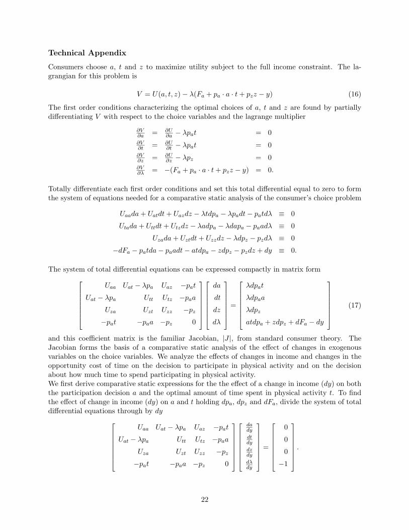
Technical Appendix

Consumers choose a, t and z to maximize utility subject to the full income constraint. The la-grangian for this problem is

V = U(a, t, z)− λ(Fa + pa · a · t + pzz − y) (16)

The first order conditions characterizing the optimal choices of a, t and z are found by partiallydifferentiating V with respect to the choice variables and the lagrange multiplier

∂V∂a = ∂U

∂a − λpat = 0∂V∂t = ∂U

∂t − λpat = 0∂V∂z = ∂U

∂z − λpz = 0∂V∂λ = −(Fa + pa · a · t + pzz − y) = 0.

Totally differentiate each first order conditions and set this total differential equal to zero to formthe system of equations needed for a comparative static analysis of the consumer’s choice problem

Uaada + Uatdt + Uazdz − λtdpa − λpadt− patdλ ≡ 0

Utada + Uttdt + Utzdz − λadpa − λdapa − paadλ ≡ 0

Uzada + Uztdt + Uzzdz − λdpz − pzdλ ≡ 0

−dFa − patda− paadt− atdpa − zdpz − pzdz + dy ≡ 0.

The system of total differential equations can be expressed compactly in matrix formUaa Uat − λpa Uaz −pat

Uat − λpa Utt Utz −paa

Uza Uzt Uzz −pz

−pat −paa −pz 0

da

dt

dz

dλ

=

λdpat

λdpaa

λdpz

atdpa + zdpz + dFa − dy

(17)

and this coefficient matrix is the familiar Jacobian, |J |, from standard consumer theory. TheJacobian forms the basis of a comparative static analysis of the effect of changes in exogenousvariables on the choice variables. We analyze the effects of changes in income and changes in theopportunity cost of time on the decision to participate in physical activity and on the decisionabout how much time to spend participating in physical activity.We first derive comparative static expressions for the the effect of a change in income (dy) on boththe participation decision a and the optimal amount of time spent in physical activity t. To findthe effect of change in income (dy) on a and t holding dpa, dpz and dFa, divide the system of totaldifferential equations through by dy

Uaa Uat − λpa Uaz −pat

Uat − λpa Utt Utz −paa

Uza Uzt Uzz −pz

−pat −paa −pz 0

dady

dtdy

dzdy

dλdy

=

0

0

0

−1

.

22

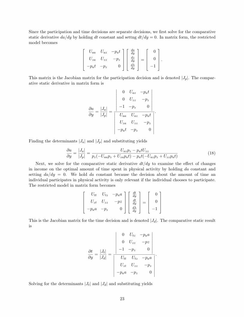
Since the participation and time decisions are separate decisions, we first solve for the comparativestatic derivative da/dy by holding dt constant and settng dt/dy = 0. In matrix form, the restrictedmodel becomes

Uaa Uaz −pat

Uza Uzz −pz

−pat −pz 0

dady

dzdy

dλdy

=

0

0

−1

.

This matrix is the Jacobian matrix for the participation decision and is denoted |Jp|. The compar-ative static derivative in matrix form is

∂a

∂y=

|Ja||Jp|

=

∣∣∣∣∣∣∣∣∣0 Uaz −pat

0 Uzz −pz

−1 −pz 0

∣∣∣∣∣∣∣∣∣∣∣∣∣∣∣∣∣∣Uaa Uaz −pat

Uza Uzz −pz

−pat −pz 0

∣∣∣∣∣∣∣∣∣

.

Finding the determinants |Ja| and |Jp| and substituting yields

∂a

∂y=

|Ja||Jp|

=Uazpz − patUzz

pz(−Uaapz + Uzapat)− pat(−Uazpz + Uzzpat)(18)

Next, we solve for the comparative static derivative dt/dy to examine the effect of changesin income on the optimal amount of time spent in physical activity by holding da constant andsetting da/dy = 0. We hold da constant because the decision about the amount of time anindividual participates in physical activity is only relevant if the individual chooses to participate.The restricted model in matrix form becomes

Utt Utz −paa

Uzt Uzz −pz

−paa −pz 0

dtdy

dtdy

dλdy

=

0

0

−1

This is the Jacobian matrix for the time decision and is denoted |Jd|. The comparative static resultis

∂t

∂y=

|Jt||Jd|

=

∣∣∣∣∣∣∣∣∣0 Utz −paa

0 Uzz −pz

−1 −pz 0

∣∣∣∣∣∣∣∣∣∣∣∣∣∣∣∣∣∣Utt Utz −paa

Uzt Uzz −pz

−paa −pz 0

∣∣∣∣∣∣∣∣∣

.

Solving for the determinants |Jt| and |Jd| and substituting yields

23

∂t

∂y=

|Jt||Jd|

=Utzpz − paaUzz

pz(−Uttpz + Uztpaa)− paa(−Utzpz + Uzzpaa)(19)

The opportunity cost of time affects the decision to participate in physical activity and theamount of time devoted to physical activity. Recall, pa = ca+w and pz = cz +θw. The opportunitycost of time is the wage rate w. Expanding the lagrangian to explicitly show the full cost of timespent in physical activity and all other activities is

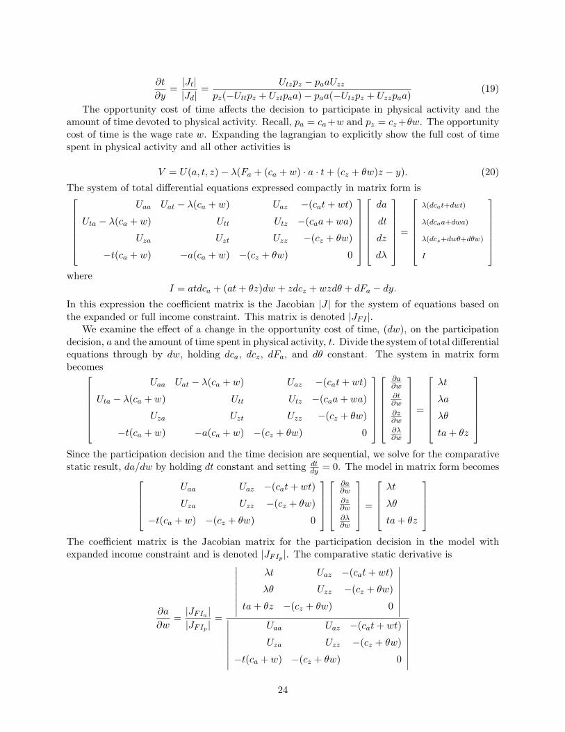
V = U(a, t, z)− λ(Fa + (ca + w) · a · t + (cz + θw)z − y). (20)

The system of total differential equations expressed compactly in matrix form isUaa Uat − λ(ca + w) Uaz −(cat + wt)

Uta − λ(ca + w) Utt Utz −(caa + wa)

Uza Uzt Uzz −(cz + θw)

−t(ca + w) −a(ca + w) −(cz + θw) 0

da

dt

dz

dλ

=

λ(dcat+dwt)

λ(dcaa+dwa)

λ(dcz+dwθ+dθw)

I

where

I = atdca + (at + θz)dw + zdcz + wzdθ + dFa − dy.

In this expression the coefficient matrix is the Jacobian |J | for the system of equations based onthe expanded or full income constraint. This matrix is denoted |JFI |.

We examine the effect of a change in the opportunity cost of time, (dw), on the participationdecision, a and the amount of time spent in physical activity, t. Divide the system of total differentialequations through by dw, holding dca, dcz, dFa, and dθ constant. The system in matrix formbecomes

Uaa Uat − λ(ca + w) Uaz −(cat + wt)

Uta − λ(ca + w) Utt Utz −(caa + wa)

Uza Uzt Uzz −(cz + θw)

−t(ca + w) −a(ca + w) −(cz + θw) 0

∂a∂w

∂t∂w

∂z∂w

∂λ∂w

=

λt

λa

λθ

ta + θz

Since the participation decision and the time decision are sequential, we solve for the comparativestatic result, da/dw by holding dt constant and setting dt

dy = 0. The model in matrix form becomesUaa Uaz −(cat + wt)

Uza Uzz −(cz + θw)

−t(ca + w) −(cz + θw) 0

∂a∂w

∂z∂w

∂λ∂w

=

λt

λθ

ta + θz

The coefficient matrix is the Jacobian matrix for the participation decision in the model withexpanded income constraint and is denoted |JFIp |. The comparative static derivative is

∂a

∂w=

|JFIa ||JFIp |

=

∣∣∣∣∣∣∣∣∣λt Uaz −(cat + wt)

λθ Uzz −(cz + θw)

ta + θz −(cz + θw) 0

∣∣∣∣∣∣∣∣∣∣∣∣∣∣∣∣∣∣Uaa Uaz −(cat + wt)

Uza Uzz −(cz + θw)

−t(ca + w) −(cz + θw) 0

∣∣∣∣∣∣∣∣∣24

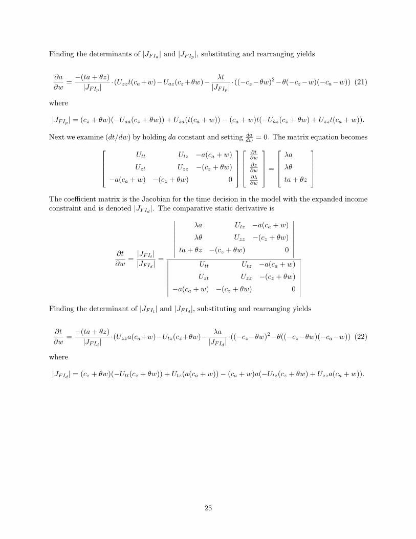
Finding the determinants of |JFIa | and |JFIp |, substituting and rearranging yields

∂a

∂w=

−(ta + θz)|JFIp |

·(Uzzt(ca +w)−Uaz(cz +θw)− λt

|JFIp |·((−cz−θw)2−θ(−cz−w)(−ca−w)) (21)

where

|JFIp | = (cz + θw)(−Uaa(cz + θw)) + Uza(t(ca + w))− (ca + w)t(−Uaz(cz + θw) + Uzzt(ca + w)).

Next we examine (dt/dw) by holding da constant and setting dadw = 0. The matrix equation becomes

Utt Utz −a(ca + w)

Uzt Uzz −(cz + θw)

−a(ca + w) −(cz + θw) 0

∂t∂w

∂z∂w

∂λ∂w

=

λa

λθ

ta + θz

The coefficient matrix is the Jacobian for the time decision in the model with the expanded incomeconstraint and is denoted |JFId

|. The comparative static derivative is

∂t

∂w=

|JFIt ||JFId

|=

∣∣∣∣∣∣∣∣∣λa Utz −a(ca + w)

λθ Uzz −(cz + θw)

ta + θz −(cz + θw) 0

∣∣∣∣∣∣∣∣∣∣∣∣∣∣∣∣∣∣Utt Utz −a(ca + w)

Uzt Uzz −(cz + θw)

−a(ca + w) −(cz + θw) 0

∣∣∣∣∣∣∣∣∣Finding the determinant of |JFIt | and |JFId

|, substituting and rearranging yields

∂t

∂w=

−(ta + θz)|JFId

|·(Uzza(ca+w)−Utz(cz+θw)− λa

|JFId|·((−cz−θw)2−θ((−cz−θw)(−ca−w)) (22)

where

|JFId| = (cz + θw)(−Utt(cz + θw)) + Utz(a(ca + w))− (ca + w)a(−Utz(cz + θw) + Uzza(ca + w)).

25