Embed Size (px)
Citation preview

IN DEGREE PROJECT ELECTRICAL ENGINEERING,SECOND CYCLE, 30 CREDITS
, STOCKHOLM SWEDEN 2019
Economic Dispatch of the Combined Cycle Power Plant Using Machine Learning
DHRUV BHATT
KTH ROYAL INSTITUTE OF TECHNOLOGYSCHOOL OF ELECTRICAL ENGINEERING AND COMPUTER SCIENCE


iii
Abstract
Combined Cycle Power Plant (CCPP)s play a key role in modern powersystem due to their lesser investment cost, lower project executiontime, and higher operational flexibility compared to other conventionalgenerating assets. The nature of generation system is changing withever increasing penetration of the renewable energy resources. Whatwas once a clearly defined generation, transmission, and distributionflow is shifting towards fluctuating distribution generation. Because ofvariation in energy production from the renewable energy resources,CCPP are increasingly required to vary their load levels to keep bal-ance between supply and demand within the system. CCPP are facingmore number of start cycles. This induces more stress on the gas tur-bine and as a result, maintenance intervals are affected.
The aim of this master thesis project is to develop a dispatch al-gorithm for the short-term operation planning for a combined cyclepower plant which also includes the long-term constraints. The long-term constraints govern the maintenance interval of the gas turbines.These long-term constraints are defined over number of EquivalentOperating Hours (EOH) and Equivalent Operating Cycles (EOC) forthe Gas Turbine (GT) under consideration. CCPP is operating in theopen electricity market. It consists of two SGT-800 GT and one SST-600 Steam Turbine (ST). The primary goal of this thesis is to maximizethe overall profit of CCPP under consideration. The secondary goal ofthis thesis it to develop the meta models to estimate consumed EOHand EOC during the planning period.
Siemens Industrial Turbo-machinery AB (SIT AB) has installed sen-sors that collects the data from the GT. Machine learning techniqueshave been applied to sensor data from the plant to construct Input-Output (I/O) curves to estimate heat input and exhaust heat. Resultsshow potential saving in the fuel consumption for the limit on Cumu-lative Equivalent Operating Hours (CEOH) and Cumulative Equiva-lent Operating Cycles (CEOC) for the planning period. However, italso highlighted some crucial areas of improvement before this eco-nomic dispatch algorithm can be commercialized.Keywords: Combine Cycle Power Plant, Equivalent Operating Hours,Equivalent Operating Cycles, Gas Turbine, Turbine Inlet Temperature,Turbine Exhaust Temperature

iv
Sammanfattning
Kombicykelkraftverk spelar en nyckelroll i det moderna elsystemet pågrund av den låga investeringskostnaden, den korta tiden för att byg-ga ett nytta kraftverk och hög flexibilitet jämfört med andra kraftverk.Elproduktionssystemen förändras i takt med en allt större andel för-nybar elproduktion. Det som en gång var ett tydligt definierat flödefrån produktion via transmission till distribution ändrar nu karaktärtill fluktuerande, distribuerad generering. På grund av variationer-na i elproduktion från förnybara energikällor finns ett ökat behov avatt kombicykelkraftverk varierar sin elproduktion för att upprätthållabalansen mellan produktion och konsumtion i systemet. Kombicykel-kraftverk behöver startas och stoppas oftare. Detta medför mer stresspå gasturbinen och som ett resultat påverkas underhållsintervallerna.
Syftet med detta examensarbete är att utveckla en algoritm för kort-tidsplanering av ett kombicykelkraftverk där även driften på lång siktbeaktas. Begränsningarna på lång sikt utgår från underhållsintervallenför gasturbinerna. Dessa långsiktiga begränsningar definieras som an-talet ekvivalenta drifttimmar och ekvivalenta driftcykler för det aktu-ella kraftverket. Kombikraftverket drivs på den öppna elmarknaden.Det består av två SGT-800 GT och en SST-600 ångturbin. Det främs-ta målet med examensarbetet är att maximera den totala vinsten förkraftverket. Ett sekundärt mål är att utveckla metamodeller för attskatta använda ekvivalenta drifttimmar och ekvivalenta driftcyklerunder planeringsperioden.
Siemens Industrial Turbo-machinery AB (SIT AB) har installeratsensorer som samlar in data från gasturbinerna. Maskininlärningstek-niker har tillämpats på sensordata för att konstruera kurvor för attuppskatta värmetillförseln och avgasvärme. Resultaten visar en po-tentiell besparing i bränsleförbrukningen om de sammanlagda ekvi-valenta drifttimmarna och de sammanlagda ekvivalenta driftcyklernabegränsas under planeringsperioden. Det framhålls dock också att detfinns viktiga förbättringar som behövs innan korttidsplaneringsalgo-ritmen kan kommersialiseras.Nyckelord: Kombicykelkraftverk, Ekvivalenta drifttimmar, Ekvivalen-ta driftcykler, Gasturbiner, Turbine Inlet Temperature, Turbine ExhaustTemperature

v
Acknowledgement
Coming to Sweden and pursue my higher education at KTH Royal In-stitute of Technology was one of the best decisions I have made. Thisshort journey is about to finish. It was my first-time experience awayfrom my home country. It is true that life begins out of the comfortzone. It was not easy to sail through this journey without the whole-hearted support of my family and friends. They have always sup-ported my choices. Their silent contribution is priceless.
I would like to thank Priyanka Shinde, who is my friend and supervi-sor at KTH for her continuous support and motivation. It was amazingto know you.
I would like to thank my examiner Mikael Amelin for his guidancethroughout my time at KTH. I still remember my first meeting withhim when I joined KTH. We had a very open discussion about courseselection. It had put my foundations for my studies at KTH.
I would like to thank Patrik Hilber, program director for Electric PowerEngineering for his continuous support and guidance right from thetime when I got admit from KTH. He has always addressed my con-cerns with an open mind and assisted me with innovative inputs.
I would like to thank my supervisors Edgar Bahilo Rodríguez andDavood Naderi for providing such an uncountable amount of knowl-edge, field expertise and rewarding guidance during this entire project.They have always given me the freedom to innovate. I will alwayscherish the wonderful discussions we used to have.
I would like to give a special thanks to Erik Ärlebäck, the managerat SIT AB who granted me this opportunity and treat me always likeone member more of the team.
Last but not least, I would like to thank Stefano Rosso and MohamedElhafiz Hassan, who were also pursuing their master thesis at SIT AB.It was always fun to have discussions with you folks.

Contents
1 Introduction 11.1 Overview . . . . . . . . . . . . . . . . . . . . . . . . . . . . 21.2 Objectives . . . . . . . . . . . . . . . . . . . . . . . . . . . 31.3 Thesis structure . . . . . . . . . . . . . . . . . . . . . . . . 3
2 Literature Review 52.1 Overview of CCPP . . . . . . . . . . . . . . . . . . . . . . 52.2 Long-term constraints in dispatch optimization . . . . . . 72.3 Modeling of combined cycle power plants . . . . . . . . . 12
3 Maximum Available Capacity of the GT 153.1 Method-1 . . . . . . . . . . . . . . . . . . . . . . . . . . . . 153.2 Method-2 . . . . . . . . . . . . . . . . . . . . . . . . . . . . 163.3 Correction . . . . . . . . . . . . . . . . . . . . . . . . . . . 18
4 Meta-models 214.1 Equivalent operating hours . . . . . . . . . . . . . . . . . 21
4.1.1 Factor Ca . . . . . . . . . . . . . . . . . . . . . . . . 214.1.2 Factor Cb . . . . . . . . . . . . . . . . . . . . . . . . 23
4.2 Equivalent operating cycles . . . . . . . . . . . . . . . . . 234.2.1 Factor Cc . . . . . . . . . . . . . . . . . . . . . . . . 234.2.2 Factor Cd . . . . . . . . . . . . . . . . . . . . . . . . 24
4.3 Meta-models . . . . . . . . . . . . . . . . . . . . . . . . . . 244.3.1 Approach-1 . . . . . . . . . . . . . . . . . . . . . . 264.3.2 Approach-2 . . . . . . . . . . . . . . . . . . . . . . 284.3.3 Required level of accuracy . . . . . . . . . . . . . . 304.3.4 Inclusion of the fast start (Fast Start (FS)) . . . . . 334.3.5 Model of Cd . . . . . . . . . . . . . . . . . . . . . . 34
5 Meta-model validation 36
vi

CONTENTS vii
6 Optimization 406.1 Selection of the CCPP . . . . . . . . . . . . . . . . . . . . . 406.2 Implementation of meta models . . . . . . . . . . . . . . . 416.3 Cost related to EOH and EOC . . . . . . . . . . . . . . . . 436.4 I/O curves . . . . . . . . . . . . . . . . . . . . . . . . . . . 44
6.4.1 I/O curves for GT . . . . . . . . . . . . . . . . . . 446.4.2 I/O curves for ST . . . . . . . . . . . . . . . . . . . 45
6.5 Case studies . . . . . . . . . . . . . . . . . . . . . . . . . . 456.5.1 Minimize total fuel consumption . . . . . . . . . . 456.5.2 Minimize total operating cost . . . . . . . . . . . . 466.5.3 Maximize total operating profit . . . . . . . . . . . 46
6.6 Optimization problem . . . . . . . . . . . . . . . . . . . . 466.7 Optimization solver . . . . . . . . . . . . . . . . . . . . . . 51
6.7.1 Optimality tolerance . . . . . . . . . . . . . . . . . 516.7.2 Warm start . . . . . . . . . . . . . . . . . . . . . . . 52
7 Results 537.1 Minimize total fuel consumption . . . . . . . . . . . . . . 537.2 Minimize total operating cost . . . . . . . . . . . . . . . . 557.3 Maximize total operating profit . . . . . . . . . . . . . . . 56
8 Conclusion and Further Studies 66
Bibliography 69
I Appendix 72
A Linear regression 73A.1 Simple linear regression . . . . . . . . . . . . . . . . . . . 73A.2 K-fold cross verification . . . . . . . . . . . . . . . . . . . 75A.3 Imbalance in data set . . . . . . . . . . . . . . . . . . . . . 76
B Pyomo 79B.1 Overview of Pyomo . . . . . . . . . . . . . . . . . . . . . . 79
B.1.1 Abstract and concrete Models . . . . . . . . . . . . 79B.1.2 Pyomo components . . . . . . . . . . . . . . . . . 80
B.2 Structured modeling with blocks . . . . . . . . . . . . . . 81B.3 Generalized disjunctive programming . . . . . . . . . . . 82B.4 Pyomo examples . . . . . . . . . . . . . . . . . . . . . . . 83

viii CONTENTS
B.4.1 The warehouse location problem . . . . . . . . . . 83B.4.2 Constraints formulation using disjuncts . . . . . . 86

List of Figures
2.1 Functioning of CCPP [3] . . . . . . . . . . . . . . . . . . . 62.2 Various configurations of CCPP . . . . . . . . . . . . . . . 72.3 Operation of the gas turbine [5] . . . . . . . . . . . . . . . 82.4 Optimization logic [5] . . . . . . . . . . . . . . . . . . . . 92.5 Integrated methodology for optimizing CCPP operation
[9] . . . . . . . . . . . . . . . . . . . . . . . . . . . . . . . . 122.6 State space transition diagram [12] . . . . . . . . . . . . . 14
3.1 Correlation Matrix . . . . . . . . . . . . . . . . . . . . . . 173.2 Histogram of α . . . . . . . . . . . . . . . . . . . . . . . . 19
4.1 Box model for maintenance plans . . . . . . . . . . . . . . 254.2 Historical data . . . . . . . . . . . . . . . . . . . . . . . . . 264.3 Method to develop the meta models . . . . . . . . . . . . 274.4 Approach - 1 . . . . . . . . . . . . . . . . . . . . . . . . . . 274.5 Estimated Turbine Inlet Temperature (TIT) from % load . 284.6 Estimated Turbine Exhaust Temperature (TET) from mea-
sured TIT . . . . . . . . . . . . . . . . . . . . . . . . . . . . 284.7 Approach - 2 . . . . . . . . . . . . . . . . . . . . . . . . . . 294.8 Estimated TET from % load . . . . . . . . . . . . . . . . . 304.9 Estimated TIT from measured TET . . . . . . . . . . . . . 304.10 Histogram of TIT . . . . . . . . . . . . . . . . . . . . . . . 314.11 Variation in residuals . . . . . . . . . . . . . . . . . . . . . 324.12 Meta model used in the optimization process . . . . . . . 334.13 Approach to estimate E[Cd] . . . . . . . . . . . . . . . . . 34
5.1 Approach to estimate EOC and EOH . . . . . . . . . . . . 365.2 Estimated and Measured EOC and EOH for GT01 . . . . 375.3 Estimated and Measured EOC and EOH for GT02 . . . . 38
ix
x LIST OF FIGURES
6.1 Active load for power plant under consideration . . . . . 416.2 Inclusion of meta models with approach 1 . . . . . . . . . 416.3 Inclusion of meta models with approach 1 and 2 . . . . . 426.4 I/O curves for GTs . . . . . . . . . . . . . . . . . . . . . . 446.5 Case studies . . . . . . . . . . . . . . . . . . . . . . . . . . 45
7.1 Results: S1, week - 1, month - 1 . . . . . . . . . . . . . . . 587.2 Results: S3, week - 1, month - 1 . . . . . . . . . . . . . . . 597.3 Results: S7, week - 1, month - 1 . . . . . . . . . . . . . . . 607.4 Results: S8, month - 1 . . . . . . . . . . . . . . . . . . . . . 617.5 Results: S9, week - 1, month - 2 . . . . . . . . . . . . . . . 627.6 Results: S9, month - 2 . . . . . . . . . . . . . . . . . . . . . 637.7 Results: S13 (cost/EOH = 1.0 pu), week - 1, month - 1 . . 647.8 Results: S14 (cost/EOH = 0.1 pu), week - 1, month - 1 . . 65
A.1 Best fitted line [20] . . . . . . . . . . . . . . . . . . . . . . 75A.2 K-fold cross validation . . . . . . . . . . . . . . . . . . . . 76A.3 Re-sampling techniques [23] . . . . . . . . . . . . . . . . . 77
B.1 Model construction process [24] . . . . . . . . . . . . . . . 80B.2 Multi-period planning problem [24] . . . . . . . . . . . . 81B.3 Formulation of warehouse problem in Pyomo . . . . . . 85B.4 Constraint formulation using disjuncts in Pyomo . . . . . 87

List of Tables
2.1 Operating Modes of CCPP . . . . . . . . . . . . . . . . . . 13
4.1 Relationship between TIT and Ca . . . . . . . . . . . . . . 224.2 Relationship between TET and Cc . . . . . . . . . . . . . . 234.3 Type of unloading event and Cd . . . . . . . . . . . . . . . 24
5.1 Consumed EOH and EOC for the planning period (fromhistorical data) . . . . . . . . . . . . . . . . . . . . . . . . . 38
7.1 Summary of results (minimize total fuel consumption) . 547.2 Summary of results (minimize total operating cost) . . . 55
B.1 Cost of delivery from warehouse m to customer n . . . . 83
xi

List of Abbreviations
S+ Start. 36
S− Stop. 36
CCC Combined Cycle Component. 13, 14
CCM Combined Cycle Mode. 13, 14
CCPP Combined Cycle Power Plant. iii, vi, vii, ix, xi, 2, 3, 5–8, 12–14,17, 40, 43–46, 52, 53, 55, 56, 66–68, 82
CEOC Cumulative Equivalent Operating Cycles. iii, 24, 43, 45, 52–55
CEOH Cumulative Equivalent Operating Hours. iii, 24, 43, 45, 52–55
CIT Compressor Inlet Temperature. 53, 54, 67
ENS Energy Not Served. 46, 55, 57
EOC Equivalent Operating Cycles. iii, vii, ix, xi, 2–4, 21, 23–25, 31, 33,34, 36–43, 45–49, 52–56, 66–68, 77
EOH Equivalent Operating Hours. iii, vii, ix, xi, 2–4, 8, 21, 22, 24, 25,29–31, 33, 35–43, 45–49, 52–56, 66, 68, 77
FFH Factored Firing Hours. 9
FL Full Load. 18, 19
FS Fast Start. vi, 23, 33
GT Gas Turbine. iii, vi, vii, x, 6, 7, 9, 10, 15–20, 23, 25, 40, 43–47, 49,53–56, 66–68
xii

List of Abbreviations xiii
HRSGT Heat Recovery Steam Generator. 6, 7, 45, 67
I/O Input-Output. iii, vii, x, 44, 45
MILP Mixed Integer Linear Programming. 3, 51, 52
PPO Power Plant Operator. 3, 22, 23, 31, 43, 55
SIT AB Siemens Industrial Turbo-machinery AB. iii, 1–3, 40, 43, 45,46
ST Steam Turbine. iii, vii, 2, 6, 7, 13, 44–46, 49, 50, 53, 55, 67
TET Turbine Exhaust Temperature. ix, xi, 23, 25–31, 33, 37, 41, 42, 66,77
TIT Turbine Inlet Temperature. ix, xi, 15, 16, 19, 21, 22, 25–33, 37, 41,42, 66, 77
UC Unit-commitment. 36
UL Unloading. 24
VER Variable Energy Resources. 2


Chapter 1
Introduction
Siemens Industrial Turbo-machinery AB (SIT AB) in Sweden is part ofthe Siemens Energy Sector. The Energy Sector is the world’s leadingsupplier of products, services and solutions for the generation, trans-mission and distribution of power and for the extraction, conversionand transport of oil and gas. Combined cycle power plants play a keyrole in modern power system due to their lesser investment cost, lowerproject execution time, and higher operational flexibility compared toother conventional generating assets. The nature of generation systemis changing with ever increasing penetration of the renewable energyresources. What was once a clearly defined generation, transmission,and distribution flow is shifting towards fluctuating distribution gen-eration. Because of variation in energy production from the renewableenergy resources, CCPP are increasingly required to vary their loadlevels to keep balance between supply and demand within the sys-tem. This induces more stress on the gas turbine and as a result, main-tanance interval is affected. The aim of this master thesis project isto develop a dispatch algorithm for the short-term operation planningfor a combined cycle power plant which also includes the long-termconstraints. The long-term constraints govern the maintenance inter-val of the gas turbines. delivers gas turbines, steam turbines, turn-keypower plants, service and components for heat and power production.
In an attempt to maintain its prominent role as one of the lead-ing turbo machinery manufacturers, increase its business intelligence;expand the offered range of services, and to create the value for itscustomers, SIT AB has taken a step forward to utilize the vast amountof precious data resource, collected from sensors that are installed in
1

2 CHAPTER 1. INTRODUCTION
the operating machines all over the world. This master thesis is per-formed in the data analytics department in SIT AB. The data analyticsdepartment has been working extensively using this data to automatedecision making process for the power plants operators, as well as toprovide useful information to other departments within SIT AB.
1.1 Overview
This Master thesis is part of SIT AB efforts done to develop decisionsupport algorithms to help the power plant operators in their daily lifewith the decisions they need to take. The final goal of the project is todevelop a mathematical model that maximizes the profit of the powerplant if they are selling all their electricity in the day ahead electric-ity market. The inclusion of any bilateral contracts, spinning reserves,and up and down regulation capacity of the power plant under con-sideration is not in the present scope of this master thesis.
The idea of this master thesis is to develop a constrained optimiza-tion model for the combined cycle power plant (CCPP) that optimizesthe dispatch of the power plant under consideration. The modeling ofCCPP is quite challenging due to the tight interaction between the gasturbine and the steam turbine (ST). Furthermore, constraints regardingthe maximum available capacity, minimum operating time, start-uptime, start-up cost, ramp rate, power balance, and maintenance shallbe considered.
One of the reasons to incorporate maintenance cost in the opti-mization model is increasing penetration of variable energy resources(Variable Energy Resources (VER)). VER are fluctuating in nature andhence, it also affects the production cost of dispatchable machines.Variation in VER is likely to change the operating point of machineswhich may not be the operating point that offers the best efficiency.Furthermore, number of operating cycles for any machine is also in-creased due to the variation in VER. This puts stress on the mechanicalcomponent of the machine which ultimately results into more frequentmaintenance and hence, an effort shall be made in this master thesis tocapture the cost associated with the maintenance.
In addition to this, there are two more ongoing master thesis projectsat SIT AB. First project emphasizes on developing economic dispatchalgorithm for a CCPP without any constraints on EOH and EOC to
CHAPTER 1. INTRODUCTION 3
minimize the total fuel consumption during the planning period. Sec-ond project emphasizes on forecasting of electricity price and fuel costusing various machine learning methods. The idea is to integrate theseprojects with the previous work done at SIT AB in an attempt to de-velop an end to end decision support tool for the Power Plant Operator(PPO).
1.2 Objectives
The present master thesis project aims to:
• The need of inclusion of the long-term operational constraints inthe short-term operation planning of the CCPP.
• Study the in-house models to estimate the equivalent operatinghour (EOH) and equivalent operating cycle (EOC) for the gasturbine under consideration.
• Identify the power plant to perform the studies
• Estimate the maximum available capacity of the gas turbines forthe power plant under consideration.
• Develop meta-models to link the output of the dispatch opti-mization algorithm to the the parameters that influence EOH andEOC consumption using machine learning techniques.
• Develop mathematical mixed integer linear programming (MixedInteger Linear Programming (MILP)) using Pyomo.
• Describe the need of future studies and areas of further improve-ments at SIT AB.
1.3 Thesis structure
• Chapter 2 gives an overview about the previous studies done inthe area of unit-commitment problem formulation for the com-bined cycle power plants. Reader is envisaged to refer this toget brief idea about the topic. This section also gives brief ideaabout functioning of a CCPP along with typical configurations ofa CCPP.

4 CHAPTER 1. INTRODUCTION
• Chapter 3 explains about the estimation of the maximum avail-able capacity for the gas turbine. The maximum amount of powerthat a gas turbine can produce is a function of ambient conditionsand hence, it is envisaged to use the maximum available capacityas an upper bound of the generation constraint instead of usingthe fixed rated value of the gas turbine.
• Chapter 4 gives the idea about the life of the gas turbine underconsideration. It introduces the concept of equivalent operat-ing hours (EOH) and equivalent operating cycle (EOC). Further-more, meta-models to estimate the parameters influencing theEOH and EOC are explained.
• Chapter 5 validates the models developed to estimate EOH andEOC. Furthermore, analysis of actual measurements and esti-mated values is represented.
• Chapter 6 highlights about selection of the power plant followedby the optimization model developed for this project. It also ex-plains about some features of the optimization solver.
• Chapter 7 discusses about the results obtained from the opti-mization algorithm along-with some sensitivity analysis to ob-serve the change in the dispatch results with respect to any changein the input parameters.
• Chapter 8 draws the conclusion of the study along with the areaof further studies.
• Appendix A provides an idea about the linear regression tech-nique used in the machine learning. It also explains about theK-fold validation and imbalance in the data set.
• Appendix B introduces the programming in Pyomo to formu-late the dispatch optimization problem with relevant examples.Basic syntax about coding is also explained here for the betterunderstanding of the reader.

Chapter 2
Literature Review
This section highlights of the background concepts of the thesis topic.It is envisaged to go through to make yourself familiar about impor-tant concepts about the topic. Gas-fired power plants have been animportant part of power systems for several decades. The success ofgas-fired power plants has been motivated by, among other things,their shorter construction times, lower investment cost and higher ef-ficiency and flexibility compared to other power generation technolo-gies [1], [2]. Furthermore, the gas will become more prevalent due tothe increased production in shale gas. Literature review is divided inthree sections. Section 2.1 gives brief idea about operation of a CCPP.Section 2.2 explains about need of inclusion of long-term constraints inthe dispatch optimization problem along with some useful approachesfor modeling. Section 2.3 explains about different models to formu-late the unit commitment problem for the combined cycle power plant(CCPP).
2.1 Overview of CCPP
This section provides brief overview about functioning of a CCPP.A CCPP uses both a gas turbine and a steam turbine to produce thepower.
A CCPP relies on the simple fact that a gas turbine produces bothpower and hot exhaust gases. The compressor sucks the air from theatmosphere at ambient conditions. CCPP can also have provision ofpre-cooling systems like a chiller to reduce the temperature of the air.It increases the air density and increases the air mass flow to the com-
5

6 CHAPTER 2. LITERATURE REVIEW
pressor. Air is compressed in the compressor. The compressor is oftenconnected to the shaft of the GT. This means that a part of power gen-erated by the GT is consumed by the compressor. Hot compressedair is mixed with the fuel. The hot air-fuel mixture moves throughthe gas turbine blades, making them spin. The generator connectedwith GT produces the electric power. In a CCPP, the exhaust gas fromthe GT is directed to the heat recovery steam generator Heat RecoverySteam Generator (HRSGT). HRSGT produces the super-heated steam.HRSGT can also have the auxiliary firing system with supplementaryfuel to supply more heat to the water. The high pressure super-heatedsteam is delivered to the ST where it will expand and produce the me-chanical power. The ST is connected to the generator to produce theelectric power. The functioning of a CCPP is represented in figure 2.1.
Figure 2.1: Functioning of CCPP [3]

CHAPTER 2. LITERATURE REVIEW 7
The configuration of CCPP can vary from plant to plant. Let usassume that a CCPP has two GTs. It is possible to have single or sepa-rate HRSGT for both of the GTs. If there are separate HRSGTs for theGTs, it is possible to have single or separate ST connected to HRSGTsystem. This is visualized in figure 2.2. Combination of GT along withits ST is described as a block. The CCPP under consideration has con-figuration - 2 in reality. However, it is modeled as configuration - 3 forthis project. It is due to lack of availability of data regarding HRSGT.
Figure 2.2: Various configurations of CCPP
2.2 Long-term constraints in dispatch opti-mization
Presently in electric power systems, an emphasis is being put on pro-viding low-carbon energy while ensuring security and supply. Therising share of the renewable generation has reduced the load factorof the CCPP. However, these renewable generation sources are inter-mittent and not dispatchable. CCPP technology is more flexible owingto the lower star-up time and faster ramping rates. Therefore, CCPPpower plants are having an increased number of start-ups during ayear. Traditionally, CCPP plants are designed for the base-load opera-tion with the limited number of start-ups in a year. Start-ups and shut-downs cause the variation in the boundary conditions. This causesvariation in the stress throughout the material of each component. Dueto the increased number of start-ups in the current scenario, the CCPP

8 CHAPTER 2. LITERATURE REVIEW
plant owners are facing higher maintenance costs. Therefore, it is es-sential to include the long-term constraints to optimize the short-termoperation of the power plant in order to maximize the overall profit.
Long term maintenance optimization of CCPP plants in Spain isanalyzed in [4]. During 2006 to 2010, the installed capacity of CCPPis increased. However, the relative energy supplied is decreased. Fur-thermore, the number of starts is increased. [4] presents a formula-tion of a mixed-integer mathematical optimization problem that in-corporates the long-term maintenance constraint and daily operationto minimize the total operation cost of a power plant under consider-ation. The operating hours are classified into valley and peak hours asit might be beneficial to run the power plant when the electricity priceis less during the valley hours to avoid the maintenance cost due to thecyclic operation. This paper uses the concept of the equivalent oper-ating hours (EOH) to formulate the maintenance constraint however,the estimation of EOH is not analyzed in detail.
Figure 2.3: Operation of the gas turbine [5]
One of the patent applications by GE [5], leverages ambient andmarket forecast data as well as asset performance and part-life to gen-erate the operating schedule that maximizes the profit subjected to theoperating constraints and the part-life constraint. It is developed on

CHAPTER 2. LITERATURE REVIEW 9
the concept of a hot load path and cold load path operation. As rep-resented in figure 2.3, the gas turbine can produce the same amountof output power at various temperatures. This flexibility is exploitedhere. When the turbine produces power at a higher temperature it re-sults in higher efficiency, but it also consumes more part life becauseof higher working temperature. On the other hand, the cold load op-eration results in lower efficiency but consumes lower part life. There-fore, the choice of operation is a trade-off between the efficiency andthe part life consumption.
Sometimes, the plant operator can peak-fire the gas turbine to pro-duce more output to above the base capacity during the peak hours tomake more profit at the expense of faster part-life consumption. Thismay also result in shorter maintenance intervals. In this patent, theoperational impact on the part life is considered by defining the fac-tored fired hours (Factored Firing Hours (FFH)) and the maintenanceintervals are defined over FFH. Every hour when the GT is operatedup to its base capacity, 1 FFH is consumed from the part life. However,when the GT is operated in a peak-fire mode to produce more power,1 hour of operation is more than 1 FFH. Such operation will result inreduced maintenance interval. The plant operator can compensate thisby operating the GT in cold part-loading in some hours. 1 hour of suchoperation will result in less than 1 FFH. Such operation will increasethe maintenance interval but will offer lower efficiency.
Figure 2.4: Optimization logic [5]
The cold path operation results in the generation of the FFH whilethe hot path operation results in increased consumption of the FFH.

10 CHAPTER 2. LITERATURE REVIEW
Cold path operation has lower efficiency and hence, increased fuelconsumption whereas peak fire operation increases the maintenancecost due to shortened maintenance interval. It is also important toconsume the part life before the maintenance else it will result in theloss of part life. The idea of dispatch optimization represented in [5]utilizes the balance between the creation and consumption of part-lifecredits across the scheduled maintenance interval by determining theoptimal hours for cold path and hot path operation. Figure 2.4 rep-resents the optimization logic. Readers are envisaged to refer [5] formore technicalities.
Doctoral thesis in [6] emphasizes the reliability-based maintenancescheduling for the gas turbines. Though it is not directly related todispatch optimization, it gives valuable insights about the importanceof the part-life estimation. There are several damage mechanisms forthe GT parts, and this makes the GT unreliable. The wear out can leadto failure of parts and hence, unplanned outages. Therefore, it is es-sential to keep track of the part’s life consumption to plan the outages.The maintenance concepts for the GT are based on one life counter i.e.number of firing hours or factored firing hours or equivalent operat-ing hours. This is relatively convenient to plant the outages, but it hassome disadvantages. If the planned outage falls when the electricityprices are high, the plant operator has two options. Either the operatorcan proceed with the outage and lose the opportunity to make moreprofit or prepone the outage and lose the remaining part life. Fur-thermore, multiple life counters for that includes the various turbineparts are envisaged to maximize the life consumption of various parts.However, having multiple life counters makes the outage coordinationchallenging as it is beneficial to combine the outages of different partsdue to dependencies in the dismantling process.
One of the patent applications by Siemens [7], emphasizes the in-tegrated optimal outage coordination in the energy delivery system.The electricity markets generally include two types of commodity i.e.power and energy. Markets for energy trade net generation output forthe number of intervals by the supplier and the consumer. Marketsfor power are managed by the market operators to ensure reliability.It includes ancillary services. Repair and maintenance of the systemcomponents result in scheduled outages in the system. It is impor-tant to coordinate these outages without compromising the system’ssecurity and stability. Outages also result in a change in the marginal
CHAPTER 2. LITERATURE REVIEW 11
cost which will also affect the electricity price. Therefore, coordinatingthe outages is more of an iterative process in which the system oper-ator solves the complex optimization process to approve the outagerequests by the asset owners.
Various methods to model the major overhaul cost of gas-fired plantin the unit commitment problem are represented in [8]. Traditionally,the operation and maintenance O&M costs were introduced in the unitcommitment problem by adding an additional cost adder component.O&M costs are reflected in the long-term service agreements. It can bemodeled as a function of the number of firing hours and the number ofstarts. The traditional approach of modeling the O&M costs assumesa lower number of starts. However, when the gas turbine has a greaternumber of starts, cyclic stress is more on the components. The inad-equacy of modeling of O&M cost in the unit commitment problem ishighlighted by PJM, ERCOT, and CAISO. Three modeling approachesto formulate the maintenance interval function are discussed in thispaper.
Modeling of the fatigue cost due to the cyclic operation of the gasturbines is studied in [9]. Models for the estimation of the fatigue costsis developed along with feasible transition modes. These models arelater introduced in the unit commitment problem. Figure 2.5 repre-sents the overall idea behind this process.
Research paper presented in [10] gives highlights about formulat-ing dynamic costs related to the related to start-up and ramping. Lin-ear, piece-wise linear, and step-shaped cycling costs functions are cre-ated to capture the costs related to the cycling operation in the dispatchoptimization. It gave ideas about the importance of having differentstates in the optimization algorithm. In this thesis, this is achieved byimplementing generalized disjunctive programming in Pyomo. Moredetails about Pyomo is explained in the following chapters.
Master thesis presented in [11] highlights about inclusion of long-term constraints in short-term operation planning by including the usevalue to reflect the opportunity cost. It investigates the dispatch resultsobtained from DiMOI and MaStock. The used value is a way to valuean asset scarcity by assessing the would-be future profits. Asset inscarcity is referred as a stock. It can be number of operating hours orcycles for the gas turbine. In a first phase, the optimization phase, theBellman values for the opportunity cost is calculated. In the secondphase, the simulation phase, the optimal functioning to operate the

12 CHAPTER 2. LITERATURE REVIEW
Figure 2.5: Integrated methodology for optimizing CCPP operation [9]
power plant is generated.
2.3 Modeling of combined cycle power plants
This section gives brief information about the research work done inthe area of modeling of combined cycle power plants. Inclusion ofcombined cycle plants into the unit commitment is challenging due toclose interdependence between the operation of the gas turbine andthe steam turbine. In the combined cycle power plant, the exhaustheat from the steam turbine is utilized to heat the water. However,it takes time to achieve the steam parameters before it can be used togenerate power. For example, if the power plant is in a cold state i.e.all the machines were out of operation for a considerable amount oftime then the steam turbine generator cannot produce the power at

CHAPTER 2. LITERATURE REVIEW 13
very first-time stamp when the demand arises. This physical depen-dence must be modeled in the unit commitment problem. There aremainly two types of models, combined-cycle component (CombinedCycle Component (CCC)) and combined-cycle mode (Combined Cy-cle Mode (CCM)) to formulate the unit commitment problem for thecombined cycle power plants.
[12] and [13] represents the CCM modeling approach to formulatethe mixed integer linear problem for the combined cycle units. Letus assume that there are two identical gas turbines (GT1 and GT2)and one steam turbine (ST) in a power plant. Table 2.1 lists possibleoperating modes. At any time, the CCPP can only be in one mode.
Mode Configuration
0 OFF1 GT1 or GT22 GT1 + GT23 GT1 + ST or GT2 + ST4 GT1 + GT2 + ST
Table 2.1: Operating Modes of CCPP
When CCM modeling approach is used, the constraints for thetransition between modes and minimum up and downtime must beformulated. Furthermore, not all the modes are feasible at any givenperiod. For example, the CCPP cannot go to mode 4 from mode 0 di-rectly. This is represented in figure 2.6. Each mode of operation can betreated as a pseudo unit with its own constraints. To implement CCM,it is important to have the information and data about the plant config-uration. For example, if the plant has separate heat recovery boiler foreach turbine and if the boilers have supplementary firing. It is oftenchallenging to find such detailed information about the plant.
CCC modeling approaching for CCPP is investigated in [14] and itsresults are compared with the results obtained using the CCM model.In the CCC model gas turbines and steam turbines are considered asan individual component rather than considering them as operatingmodes. Input-output (IO) curves of components are included in themodel. The results obtained from CCM models gives the power out-put of each mode at each time stamps. However, the plant operatormust divide it among the generators based on the experience which

14 CHAPTER 2. LITERATURE REVIEW
Figure 2.6: State space transition diagram [12]
may not be optimal. On the other hand, CCC models will give the out-put from each component individually. Most of the time, it is possiblethat the CCPP is operating in a certain mode. Under such a scenario,there will not be enough data points for other modes of operation tomodel them accurately. One of the disadvantages of the CCM modelsis the number of components. As the number of components increases,the number of operating modes will also increase. This increases thecomplexities in mapping the state transitions. In CCM model, degra-dation of any component will affect multiple operating modes andhence, it asks for re-calibration of all modes to include the effects ofdegradation. While in CCC models, the only component of interestcan be re-calibrated. It is also highlighted that CCM models have agreater number of integer variables and constraints compared to CCCmodels. This also increases the computational cost.
In this thesis CCC modeling approach is used as the data of heatrecovery boiler is not available. Furthermore, the main objective ofthis thesis is to include machine life in the unit commitment problem.

Chapter 3
Maximum Available Capacity ofthe GT
It is important to estimate the maximum available capacity of the gasturbine as it sets the generation constraints. If it is under-estimated,then the machine may not produce the power that it can produce, andthis results in the monetary loss for the power plant owner. In a similarway, if it is overestimated then it will seriously affect the life of themachine and personal safety. In this thesis, two methods to estimatethe maximum available capacity are investigated.
3.1 Method-1
There is a signal for % load in the system. Method to calculate thissignal is developed internally by using three parameters. These pa-rameters are available only in the internal report. However, these pa-rameters are related to the following phenomenon.
• Parameter A is related to the density of the air hence, with thenumber of air molecules per kg that go through the compressor.
• Parameter B is related to the effective area of the compressor,therefore, the mass flow of the air that goes through the com-pressor.
• Parameter C is related to the turbine inlet temperature (TIT) dur-ing combustion process and with the turbine efficiency.
15

16 CHAPTER 3. MAXIMUM AVAILABLE CAPACITY OF THE GT
While checking these values, it was found that there were so manymissing values (Not a Number). This is because the algorithm used tocalculate % load considers the value of TIT in degree Celsius however,the measurement is reported in degree Fahrenheit. Therefore, insteadof using the % load values directly, it is calculated using the same al-gorithm with the TIT measurement converted to degree Celsius.
While investigating the calculated values of % load, it was foundthat some of these values were not realistic. For example, the calcu-lated value of % load is 100 but the value of parameter B at that time-stamp is not maximum. When the gas turbine is operating at 100 %load, the value of parameter B must be at its highest value to offer themaximum effective area to get highest air mass flow. Furthermore, theactive power load was also lower than its maximum rated capacity andhence, such values of % load must be corrected. However, the value ofTIT is near its maximum rated value. This leads to one hypothesis thatthe way % load is calculated here represent the thermal loading of themachine than the power loading. However, further investigation intothis is not in the scope of this thesis work and is subjected to futureresearch. Maximum available capacity can be calculated by dividingthe active power load by the % load as represented in equation 3.1.
MaxCapmethod1 =ActiveLoad
%Load[MW ] (3.1)
3.2 Method-2
The performance of the gas turbine is dependent on the operatingconditions. This issue of having varying thermal efficiency has beenconsidered by gas turbine manufacturers by means of ISO-rating stan-dards (ISO 19859:2016). The ISO rating algorithm allows calculatingthe performance in real-time considering the operating ambient con-ditions.
Some of these parameters are directly related to the density of theair and hence, any change in ambient condition from the ISO condi-tions will affect the performance of the gas turbine. This is mainlybecause of the change in the air density and therefore the mass flow ofthe air. Therefore, the maximum power that can be produced by thegas turbine is a function of the ambient conditions.
Increases in the ambient temperature can highly affect the gas tur-

CHAPTER 3. MAXIMUM AVAILABLE CAPACITY OF THE GT 17
bine performance. When the inlet air is hot the net power of the gasturbine reduces. For every 1 ◦C increment in the ambient temperature,the amount of the reduction in power output is nearly 0.9% (Petch-ers, 2002). Air density reduces with increase in the temperature. Thisreduces the air mass flow which will result in reduced output power.
With decrease in the barometric pressure, the air density reduced.As a result, the air mass flow rate reduces which in turn reduce theoutput power.
The atomic mass of the H2O is less than N2 and O2. Due to thatreason mass of the humid air is less than the mass of the dry air (samevolume). Therefore, the humid air has less density than the dry air. Asa result of low-density air, the amount of dry air mass entering the gasturbine reduces. Thus, the performance of the gas turbine reduces.
Figure 3.1 represents the correlation matrix for the GTs for the CCPPunder consideration. This is also used to estimate the heat input andexhaust heat using multiple linear regression in chapter 6.
Figure 3.1: Correlation Matrix
Few important parameters that affect the performance of the gasturbine are as below.
• Ambient temperature (T0)
• Relative humidity (RH)
• Barometric pressure (P0)

18 CHAPTER 3. MAXIMUM AVAILABLE CAPACITY OF THE GT
• Inlet pressure losses (Pi)
• Outlet pressure losses (Po)
• Power factor correction (PF )
• Fuel quality (Fq)
Each variable is represented by a coefficient Ci. An overall parame-ter is a multiplication of individual parameters as represented in equa-tion 3.2. Furthermore, the value of each parameter is calculated usingpolynomials over their range. These polynomials are part of an inter-nal report and are strictly confidential.
CPower = CT0 ∗ CRH ∗ CP0 ∗ CPi∗ CPO
∗ CPF ∗ Cfq (3.2)
MaxCapmethod2 = Cpower ∗ PN [MW ] (3.3)
Where,PN = Nominal power [MW]
In this thesis, CT0 , CRH , C(P0 are used to estimate the Cpower as thequality of these signal is good. These signals are for ambient condi-tions that can be forecasted. Therefore, the maximum available ca-pacity can be estimated for the planning period using the forecastedambient conditions.
3.3 Correction
As highlighted in the previous sections, method 1 lacks accuracy forsome values of % load near 100%. While method 2 does not considerall parameters, which affects the maximum available capacity of themachine. This section describes the method used to correct the max-imum available capacity to use it further to develop the meta modelsin the next chapter.
There is one signal “full load operation (Full Load (FL))”. It is abinary signal. When it is ‘1’, the machine is operating at its full loadcapacity and hence, when the FL signal is ‘1’, the active power loadcan be considered as the maximum available capacity. At this timeinstance % load = 100%

CHAPTER 3. MAXIMUM AVAILABLE CAPACITY OF THE GT 19
Let, α =ActivePowerFL=1
MaxCapmethod2(3.4)
α is defined to quantify the error in the maximum available capac-ity and the active power output when FL = 1. These two must be thesame when FL = 1. Figure 3.2 represents the distribution of α.
Figure 3.2: Histogram of α
Mean value of α is used to estimate the maximum available capac-ity at each time-stamp as represented equation 3.5.
MaxCapt =MaxCapmethod2
t
αmean
(3.5)
When a single mean value of α is used to estimate the maximumavailable capacity, there were some instants when the maximum avail-able capacity was less than the active power load of the generator. Thisis mathematically logical. Furthermore, the machines were not doingthe peaking operation. This was evident as the value of TIT was notabove its nominal values. Therefore, for such instances, the maximumavailable capacity is considered to be the active power load at thattime-stamp. Such time-stamps only represent a small fraction of thehistorical data.
Finally, method 2 shall be used to estimate the maximum availablecapacity using the forecasted ambient conditions and the α correction.However, further, development is envisaged in order to develop more

20 CHAPTER 3. MAXIMUM AVAILABLE CAPACITY OF THE GT
general algorithms to estimate the maximum available capacity withthe highest accuracy.

Chapter 4
Meta-models
In this section formulation of EOH and EOC is explained. Value ofEOH and EOC at time-stamp depends on the physical operating pa-rameters and the design limits. These limits are strictly confidentialand hence, numerical values are not mentioned in this section.
4.1 Equivalent operating hours
According to the engine control specification of SGT-800, the equationto calculate the EOH is given by equation 4.1.
EOH = f(Ca, Cb, H,EOC) (4.1)
Where,Ca = Factor that depends on TITCb = Factor that depends on the type of fuelH = Number of operating hoursEOC = Equivalent operating cycles
4.1.1 Factor CaFactorCa, is dependent on the turbine inlet temperature, TIT. Based onthe type of the turbine, the limits on the TIT are set. Type of machineis the main attribute corresponding to the nominal capacity of the gasturbine. It consists of three main sections. These are the compressor,
21

22 CHAPTER 4. META-MODELS
combustor, and turbine. Each machine type has some specific charac-teristics. The power output of the gas turbine depends on the climaticconditions. Change in the ambient conditions will change the air den-sity and subsequently the pressure ratio. To compensate for this, morefuel would be required to produce the same output power. However,this will increase the turbine inlet temperature that might go above themelting point of the material used and hence, there must be an upperlimit for the turbine inlet temperature. Machine type also depends onthe type of material used in the turbine. Depending on this materialthe temperature limits for the operation is determined. For this ma-chine type, the Ca factor is given in table 4.1. The measurement unit ofTIT is ◦C. The value of Ca increases with increase in TIT.
Turbine Inlet Temperature Ca
TIT ≤ TIT1 Ca1
TIT1 < TIT ≤ TIT2 Ca2
TIT2 < TIT ≤ TIT3 Ca3
TIT> TIT3 Ca4
Table 4.1: Relationship between TIT and Ca
It is interesting to observe that the value of Ca factor is always morethan Ca1 and hence, it will always increase the EOH. This is a moreconservative approach. When the machine is operated at lower tem-peratures, Ca can be less than Ca1 . For such operation, the efficiency islikely to be less, and the fuel consumption will be more to generate thesame amount of power. However, such operation is likely to be ben-eficial when the fuel price and electricity demand faced by the powerplant is less. Under such operation, 1 hour of operation will be lesserthan 1 EOH. That means, by compromising the efficiency, the powerplant operator (PPO) can consume lesser life of the machine. This willallow PPO to consume more machine life when the electricity price ishigher. PPO can operate machines at higher temperatures to gener-ate more power at better efficiency to maximize the profit. This ideais documented well in one of the patent applications filed by the GE[5]. However, in this application, the idea is developed consideringthe firing hours only. Presently, there are no documents that highlightsuch provision for the SGT-800 and hence, in this thesis, the idea ofdeveloping the model with Ca<Ca1 is not included. However, it is sub-

CHAPTER 4. META-MODELS 23
jected to future research and development. Its inclusion will give moreflexibility to PPO to utilize the life of the gas turbines.
4.1.2 Factor CbParameter Cb is dependent on the type of fuel used during the opera-tion. For the gas fuel, Cb = Cb1 while for the liquid fuel, Cb = Cb2
4.2 Equivalent operating cycles
According to the engine control specification of SGT-800, the equationto calculate the EOC is given by equation 4.2.
EOC = f(Cc, Cd, Sup, Sdown) (4.2)
Where,Cc = Factor that depends on the type of start-up of the GTCd = Factor that depends on the type of shut-down of the GTSup = Start-up variableSdown = Shut-down variable
4.2.1 Factor CcFactor Cc depends on the turbine exhaust temperature. It is given intable 4.3. The measurement unit of TET is ◦C.
Turbine Exhaust Temperature Cc
TET ≤ TET1 Cc1
TET > TET1 Cc2
TET > TET1(FS1) Cc3
TET > TET1(FS2) Cc4
Table 4.2: Relationship between TET and Cc
The fast start - 1 and fast start - 2 are the optional features for thecustomer. While investigating the customer data, it was found thatthe machines at plant under consideration do not have these optionalfeatures.

24 CHAPTER 4. META-MODELS
4.2.2 Factor CdFactor Cd depends on the type of unloading (Unloading (UL)) eventduring the shutdown. It is given as below. It is given in table 4.3.
Unloading Event Type Cd
Normal unloading Cd1
Unloading - 1 Cd2
Unloading - 2 Cd3
Unloading - 3 Cd4
Table 4.3: Type of unloading event and Cd
Ramp-down rate during the shut down events are different. Thestress induced in the machine is proportional to the ramp-down rateduring the shutdown. Numerical relationship among different valuesof Cd represented in equation 4.3.
Cd1 < Cd2 < Cd3 < Cd4 (4.3)
4.3 Meta-models
The maintenance interval of the turbines is specified in terms of theEOH and EOC. This is referred to as a box model. There are two typesof maintenance plans for the SGT-800, basic maintenance plan, andextended maintenance plan. These plans consist of remote minor in-spection, hot gas path inspection, and major overhaul.
The basic maintenance plan offers the greatest flexibility in termsof combining the high number of starts and operating hours. It allows20,000 EOH or 1,000 EOC, whichever is earlier between hot gas pathinspection and major overhaul. This plan is adopted for normal powerplants.
The extended maintenance plan allows 30,000 EOH or 500 EOC,whichever is earlier between hot gas path inspection and major over-haul. This plan is adopted for base-load power plants. The mainte-nance plans are represented in in figure 4.1. This is used to set limiton maximum allowable CEOC for maximum allowable CEOH duringthe planning period.

CHAPTER 4. META-MODELS 25
Figure 4.1: Box model for maintenance plans
The maintenance intervals for the other parts of the turbines likecompressor and burner are different. However, in this thesis, the ma-jor focus is on the hot gas path inspection and the major overhaul. Thedispatch algorithm can easily modify to include other part life con-straints and to optimize the overall plant operation in the long-term.
It is evident that it is necessary to include EOH and EOC in theoptimization algorithm to include the part life and maintenance inter-val constraints. The result of the dispatch algorithm consists of poweroutput, unit commitment, start-up, and shut down. However, the pa-rameters used to calculate EOH and EOC uses TIT, TET, fuel type, andunloading events and hence, it is necessary to estimate these param-eters from the results of the dispatch algorithm and historical data ofthe plant. It was found that the the power plant under considerationwas always operated with the gas fuel and hence, Cb is set to be Cb1 .In the future, the type of operating fuel can be entered as a parameter.This will make the model realistic in nature.
The aim of the meta-models is to estimate the physical operatingparameters, used in EOH and EOC calculation from the result of theoptimization algorithm. % load is used as a starting point to formulatethe meta-models as % load, TIT, and TET are somehow correlated witheach other (WGT=m*Cp*(TET-TIT )). % load is calculated as shown inequation 4.4.
%Load =ActiveLoad
MaximumAvailableCapacity∗ 100[%] (4.4)

26 CHAPTER 4. META-MODELS
The meta-models are developed using the historical data and hence,they do not include the effect of degradation. Further research anddevelopment are envisaged to include the degradation in the meta-models. As % load is a base of the meta models, it is essential to esti-mate maximum available capacity as accurately as possible. As high-lighted in chapter 3, there are some errors in estimation of maximumavailable capacity.
Figure 4.2: Historical data
Figure 4.2 represents the historical data used to formulate the meta-models. Simple linear regression is used to establish the relationshipbetween the desired parameters. Furthermore, the curves are dividedin the number of regions to achieve better accuracy out of the linearregression.
Figure 4.3 represents an overall idea to develop the meta models. Inthis thesis, two approaches are checked to develop the meta-models.
4.3.1 Approach-1
As represented in figure 4.4, in this approach, TIT is estimated from %Load. TET is then estimated using TIT. TET is also estimated using themeasured value of TIT to compare the residuals in estimated TET, es-timated from the true values of TIT as well as from estimated values ofTIT. Residual is the difference between the true value of the parameterand the estimated value of the parameter.

CHAPTER 4. META-MODELS 27
Figure 4.3: Method to develop the meta models
Figure 4.4: Approach - 1
Estimate TIT from % load
Figure 4.5 represents the scatter plot of measured TIT and estimatedTIT with respect to the % load along with the residuals in the esti-mated values of TIT. The value of residual is higher at lower values of% load. This is because there are not enough data points for the linearregression as the machines are rarely operated at lower % load. Thisis also rational because the turbine offers higher efficiency when op-erated near its full load capacity. Furthermore, at lower % load, TITvalues are not so high that error in magnitude of 0.1 pu will give thewrong estimation of the Ca factor. However, this error in estimatedTIT may give more error in the estimation of TET.

28 CHAPTER 4. META-MODELS
Figure 4.5: Estimated TIT from % load
Estimate TET from TIT
Figure 4.6 represents the scatter plot of measured TET and estimatedTET with respect to TIT residuals in the estimated values of TET.
Figure 4.6: Estimated TET from measured TIT
4.3.2 Approach-2
In reality, TIT is back-calculated from TET and hence, there are chancesof error in the value of TIT due to calculation delay as well. As repre-sented in figure 4.7, in this approach, TET is estimated from % Load.

CHAPTER 4. META-MODELS 29
TIT is then estimated using TET. TIT is also estimated using the mea-sured value of TET to compare the residuals in estimated TIT esti-mated from the true values of TET as well as from estimated valuesof TET. Residual is the difference between the true value of the param-eter and the estimated value of the parameter.
Figure 4.7: Approach - 2
Estimate TET from % load
Figure 4.8 represents the scatter plot of measured TET and estimatedTET with respect to the % load along with the residuals in the esti-mated values of TET. The value of residual is higher at lower valuesof % load. This is because there are not enough data points for thelinear regression as the machines are rarely operated at lower % load.This is also rational because the turbine offers higher efficiency whenoperated near its full load capacity. This problem is referred to as theimbalanced data in data science. In the case of the imbalanced data,majority classes dominate the minority classes. This creates biased re-sults. This challenge can be addressed during the pre-processing stageby doing re-sampling. However, the same is not implemented as thefound results are satisfactory as far as the modeling of EOH is con-cerned.
Estimate TIT from TET
Figure 4.9 represents the scatter plot of measured TIT and estimatedTIT with respect to TET residuals in the estimated values of TIT.

30 CHAPTER 4. META-MODELS
Figure 4.8: Estimated TET from % load
Figure 4.9: Estimated TIT from measured TET
4.3.3 Required level of accuracy
It is always good to have the highest level of accuracy when it comesto estimating any parameter associated with the turbine operation. Inthis case, Ca andCc depend on the TIT and TET respectively. However,their values are defined over the interval therefore, if the estimatedvalues of TIT and TET in the correct interval, it is enough to estimateCa and Cc. Furthermore, the accuracy of estimated TIT must be goodas the Ca factor contributes to EOH at each time-stamp. Residuals inthe values of TIT can be observed from figure 4.5 and figure 4.9. Theaccuracy requirement for estimated TET is relatively less stringent asthere is only one break-point at TET=TET1 for the machines under

CHAPTER 4. META-MODELS 31
consideration. Furthermore, Cc will contribute EOH and EOC onlywhen there is a start-up. To further quantify this, it is important to es-timate the probability of a start-up when the residual of TET is highest.However, it is not included in the scope of this thesis. Therefore, afterinvestigation, approach 1 is finalized to use to develop meta-modelsto estimate TIT and TET.
Figure 4.10 represents the histogram of TIT of the gas turbines atplant under consideration. It is interesting to note that the machinesare never operated above TIT1. This also indicates that the PPO isnever doing peaking operation. It would be interesting to develop themeta models for the power plant that performs the peaking operationas well. It is also envisaged to test the historical data with a 1-minuteresolution to see if the value of TIT ever goes above TIT1.
Figure 4.10: Histogram of TIT
Furthermore, while performing the linear regression, the availabledata set is divided into training and test data randomly. 80% of datapoints are used to train the model while 20% of data points are usedto test the model. Since this selection of the data-points is random, itis likely to give the different value of slope and intercept. One suchexample is shown in figure 4.11.
The maximum value of the residual is way more than what is ob-tained in figure 4.5. This is because there are only a few numbers ofdata points when the value of % load is less. Under such circum-stances, the random selection of training data set is likely to give in-accurate estimation. In this thesis, values of slope and intercept that

32 CHAPTER 4. META-MODELS
Figure 4.11: Variation in residuals
gives best values of residuals is used as input parameters in the opti-mization algorithm. It is represented in figure 4.12. It is interesting toobserve that TIT is almost flat at higher load % even after 100%. Thisis not realistic. During the peaking operation, the TIT is expected toincrease. However, the plant under consideration does not have anyhistory of peaking operation and hence, there are no data points thatcan be used to model the machine’s behavior under peak operation.The machine will not generate 1.5 times its rated capacity. From figure4.12, with the current meta model, TIT will never go beyond TIT1 andhence, the value of Ca will always be Ca1 . Therefore, for this specificcase, it can be omitted from the optimization algorithm in order to re-duce the number of integer variables. However, it is kept in order toestimate the computation cost.
One approach would be to run the process of finding slope and in-tercept of the best-fitted line using the linear regression multiple timeand select the weighted average of the result. Another approach tohandle this would be to use the K-fold cross-validation. More infor-mation about this is highlighted in A. However, with the imbalance inthe data set, it is not feasible to implement the K-fold cross-validationtechnique and hence, the first approach is more suitable. In addition tothis, the random split misses the effects of degradation over the periodand hence, it is also envisaged to re-celebrate the meta-models overa period or develop more sophisticated methods to incorporate thedegradation effects inherently. Later seems more challenging as the

CHAPTER 4. META-MODELS 33
Figure 4.12: Meta model used in the optimization process
aim is to utilize the output of the optimization algorithm to calculatethe EOH.
One of the limitations of this approach of estimating the value ofTIT and TET is that there will be a fixed value of TIT and TET when %load = 0. However, when the machine is not producing any power, thevalue of TIT and TET varies a lot. This is evident from figure 4.2. Thisdoes not have any implication on the estimation of EOH and EOC.
4.3.4 Inclusion of the fast start (FS)
When there is a fast start, it will stress the machine more due to morethermal stress. However, it is challenging to make meta-model for it.One simple solution to this is to include the probability of having afast start and calculate the expected value of Cc. However, such re-sults will be biased as the probability of fast start is calculated fromthe historical data sample. The more accurate method would be tocapture the fast start is to run the optimization with a 1-minute timestamp. The developed optimization algorithm uses 15-minute data.Gas turbines can reach to its full load capacity in less than 15-minutesand hence, the optimization algorithm is less likely to capture the needof fast start to maximize the profit. If 1-minute data is used, then it islikely to increase the computation time and cost. The main aim afterdeveloping this optimization algorithm is to include the part life andthe maintenance constraints and hence, the planning duration is rela-

34 CHAPTER 4. META-MODELS
tively longer.
4.3.5 Model of CdAs highlighted in table 4.3, the value of Cd depends on the type ofunloading event which is related to the shut-down ramp rate. Typeof unloading event is selected by the plant operator. As the modeldeveloped in this thesis is using the 15-minute data, it misses the pref-erence for the unloading event furthermore, it is also not possible toassign any shutdown to the emergency shut down from the optimiza-tion model. One simple approach is to calculate the expected valueof Cd based on the probability of occurrence of the unloading events.This approach is represented in figure 4.13.
Figure 4.13: Approach to estimate E[Cd]
E[Cd] =4∑
i=1
Pi ∗ Cdi (4.5)
Where,E[Cd] = Expected value of Cd
Pi = Probability of ith type of unloading eventi = 1 for normal unloadingi = 2 for UL1 eventi = 3 for UL2 eventi = 4 for UL3 event
E[Cd] is used as a fixed parameter to calculate EOC when there is ashutdown. As this value is fixed, it is envisaged to use updated E[Cd]after the actual shut down event in real-time.

CHAPTER 4. META-MODELS 35
UL1, UL2, and UL3 are available as a digital signal in the system.However, there is no such digital signal for the normal stop. A digitalsignal for the normal stop is created using the value of active load andUL1, UL2, and UL3 signals. When the active load is changed to zeroafter the shutdown and none of the UL1, UL2, and UL3 signals havebeen set to ‘1’ then this stop is considered as a normal stop.
The data quality of UL1, UL2, and UL3 is not so good. It is observedthat sometimes this signal attains its value with some time delay. Un-der such a scenario, the type of shut down will be marked as a normalshut down as explained above. However, to investigate deeper intothe data measurement system is not in the scope of this thesis. How-ever, it is recommended to improve the data quality of these signals.
Furthermore, there were time-stamps when the value of UL1, UL2,and UL3 signals is ‘1’ even though the active power load is zero inprevious periods. Such values must be discarded. This could be dueto the aborted starts as well.
For this thesis, the accuracy requirement for the E[Cd] is not so crit-ical as it contributes to EOH only when there is a shutdown.

Chapter 5
Meta-model validation
In this section, the models developed chapter 4 to estimate EOH andEOC are validated. EOH and EOC are estimated for the time periodunder consideration using meta-models to estimate Ca, Cc, and Cd.These estimated values are then compared with the measured valuesof EOH and EOC for the validation purpose.
To compute EOH and EOC, Unit-commitment (UC), Start (S+), andStop (S−) variables are used. These variables are estimated from the %load. This is represented in figure 5.1.
Figure 5.1: Approach to estimate EOC and EOH
Figure 5.2 and figure 5.3 represent the comparison between esti-mated EOH and EOC for GT01 and GT02 for the time period underconsideration. The values of EOH are quite close to each other forGT01 however, it is not the case of GT02. This is due to the suddenspike in measured EOC for GT02. Therefore, there is an offset betweenthe measured and estimated values of EOH. Furthermore, the mea-
36

CHAPTER 5. META-MODEL VALIDATION 37
sured value of EOC is suspicious because of the spike that cannot beexplained with proper logic. It is also observed that the calculatedEOC has more steps than actual EOC. This is because, in the estima-tion of EOC, Cd always takes E[Cd] so it always contributes to EOC.However, if there is a normal stop, the value of real E[Cd] is Cd1 andthere will be only a small change in EOC value. This is not the bestapproach to estimate the EOC when the machine stops as it will in-crement EOC unnecessary for the normal stops, which are most of theshutdowns. In an optimization problem, the EOC is upper boundedfor the planning period and hence, increase EOC for the stops whichare normal must be avoided in a real case. Further research is requiredto classify the unloading event during the shutdown process.
Figure 5.2: Estimated and Measured EOC and EOH for GT01
It is also observed that the measured EOC is incremented by one atsome time stamps though the active load was zero in previous time-stamps. This is likely due to the failed starts. This hypothesis is basedon the increase in the measured value of TIT and TET during thesetime stamps. It is envisaged to have a provision in the EOC measure-ment algorithm to capture the failed start to avoid increment in EOC.From the above calculations, it is evident that accuracy in estimationof % load and therefore the maximum available capacity has the mostimportance as it is the building block to develop the meta-models.
The objective of this thesis is to develop a dispatch algorithm thatalso considers the part life consumption i.e. EOH and EOC. The al-gorithm is first implemented on the historical data. The time span

38 CHAPTER 5. META-MODEL VALIDATION
Figure 5.3: Estimated and Measured EOC and EOH for GT02
considered here is lesser than the EOH and EOC limits between themaintenance interval and hence, it will be impractical to use the max-imum value of the EOH and EOC as an upper bound constraint. Atthe same time, when the planning period is less than the maintenanceinterval, the upper bound values of EOH and EOC cannot be random.It is also an optimization in itself. However, it is excluded from thescope of work for now. Instead, the estimated values of EOH and EOCare used as a constraint. It is represented in table 5.1.
Machine EOH EOC
GT01 4,590 23GT02 2,730 20
GT01 + GT02 7,320 43Average 3,660 21.5
Table 5.1: Consumed EOH and EOC for the planning period (from historicaldata)
The drawback of assigning fixed values to EOH and EOC is thatthe obtained results may not be optimum. From table 5.1, it is evidentthat GT01 is utilized more than GT02 which may not be the optimumoperating strategy. Therefore, it is envisaged to study the results underdifferent scenario and perform the sensitivity analysis.
For a start, the upper bound of EOH is set by assuming that the ma-chine will run at full load throughout the planning period. Based on

CHAPTER 5. META-MODEL VALIDATION 39
the upper bound of EOH, the upper bound of EOC is decided linearlyfrom the box model of specific maintenance plan as shown in figure4.1.
Chapter 6
Optimization
In this section, the optimization model for the dispatch algorithm isexplained. The idea is to apply the newly developed dispatch opti-mization algorithm on the historical data to investigate the potentialsavings for the power plant under consideration. One of the customersof SIT AB is selected for this study after careful examination.
6.1 Selection of the CCPP
The major objective of this thesis is to formulate an algorithm to opti-mize the operation of CCPP subjected to the constraints on EOH andEOC along with other operating constraints. Constraints on EOH andEOC influence the maintenance interval of the GT. Therefore, it is im-portant to select the power plant that operates in the open electricitymarket. The maintenance of a captive power plant, fulfilling the de-mand of a production factory like steel mill, is primarily driven by thelocal demand. It is also envisaged to run the optimization for a longerperiod of time to see the effect of constraints on EOH and EOC andhence, it is essential to select a CCPP that offers good quality of data(i.e. data for all required signals is available) for the GTs.
The power plant under consideration has one block of the com-bined cycle. It consists of 2 SGT-800 gas turbines and 1 SST-600 steamturbine. Figure 6.1 represents the power production of the power plantunder consideration. At first glance, it is interesting to note that theGT01 is utilized more than the GT02. The results obtained from thenewly developed dispatch algorithm will be compared with the his-torical results to investigate the change in operation pattern and the
40

CHAPTER 6. OPTIMIZATION 41
Figure 6.1: Active load for power plant under consideration
fuel consumption subjected to the additional constraints on the EOHand EOC.
6.2 Implementation of meta models
In the chapter4, approach 1 is finalized to estimate the TIT and TET.However, in the optimization algorithm, the mix of approach 1 and 2is utilized to overcome the computational challenges without compro-mising on accuracy.
Figure 6.2: Inclusion of meta models with approach 1
In approach 1, TIT is estimated from % load and TET is estimated

42 CHAPTER 6. OPTIMIZATION
from the estimated value of TIT. This process uses piecewise linearregression and hence, the slopes and intercepts to estimate TIT andTET depend on the value of % load and the estimated value of TITrespectively. This is represented in figure 6.2. This process will berepeated at each time stamp and hence, the execution time is likely toincrease.
Figure 6.3: Inclusion of meta models with approach 1 and 2
To reduce the computational time, a mix of approach 1 and 2 isused. TIT and TET are directly estimated using % load. However, it isimportant to have same piecewise sections of % load to estimate TITand TET. If it is not the case, then it will be similar to the challengehighlighted above. This is represented in figure 6.3. The EOH andEOC are estimated and compared with the historical data to validatethis mixed approach. It gives the same result as given by approach1. This is because the parameters affecting EOH and EOC are definedover a range of TIT and TET.

CHAPTER 6. OPTIMIZATION 43
6.3 Cost related to EOH and EOC
Additional cost component for EOH and EOC is added in the objectivefunction. There are two approaches to add this costs. Either it can berepresented in form of an opportunity cost or a fixed cost associatedwith EOH and EOC based on the maintenance contract.
The opportunity cost to consume EOH and EOC can be explainedby an example of the hydro power planning operation. The variableoperating cost of a hydro plant is negligible. However, the hydro-generator is an energy-limited generator due to the limited amountof stored water in the reservoir. If the reservoir is full, any additionalwater will be spilled down the river. Therefore, there is no incentiveto not use the water for power production. The opportunity cost ofpower production is zero when the reservoir is full. If the reservoiris not full, the water should be used to generate electricity when theelectricity price will be higher. Therefore, the opportunity cost to con-sume the stored water at time = t, will be more is the electricity priceis less at time=t. In a similar way, the opportunity cost to consumethe stored water at time = t, will be less if the electricity price is moreat time = t. This is quite rational. One important take away from thisillustration is that the opportunity cost is dynamic in nature and is cor-related with the electricity price during the planning period. For thegas turbines, the opportunity cost to consume EOH and EOC will beless when the electricity price is higher, and it will be more when theelectricity price is less. Master thesis project presented in [11] explainsthe methodology to estimate the opportunity cost to model the effectof long-term constraints on EOH and EOC in the short-term planningproblem based on the Bellman algorithm.
Due to the limitation of time, the approach explained above wasnot implemented. Furthermore, there are constraints that limits CEOHand CEOC for the planning period. Therefore, it allows to consumeEOH and EOC in such a way that overall result is optimized. How-ever, it does not mean that there is no cost associated with EOH andEOC. Due to more cycling, CCPP is likely to reach specified limit ofEOH and EOC for the maintenance earlier. PPO is likely to have morecost of maintenance during life of the GT. For this thesis, the detailedcost of maintenance is estimated from the cost configurator that SITAB has. This cost is distributed over EOH and EOC equally. Sensi-tivity analysis is also performed to assess the effect of any change in

44 CHAPTER 6. OPTIMIZATION
the maintenance cost. As the cost related to maintenance is strictlyconfidential, the results are normalized.
6.4 I/O curves
This section gives an idea about developing I/O curves for the GT andST. Data driven approach is used to determine the I/O curves of theturbines for the CCPP under consideration.
6.4.1 I/O curves for GT
Historical data of active load and GT’s efficiency is available. Usingthis data, input heat is back calculated. Data of exhaust heat is avail-able from the system. For this thesis 15 minutes time sampled valuesare used.
As represented in figure 3.1, input heat and exhaust heat have strongcorrelation with the active load. Furthermore, ambient conditions alsoplays important role in performance of the GT. Multiple linear regres-sion technique is used to estimate heat input and exhaust heat fromactive load and ambient conditions. This is represented in 6.4.
Figure 6.4: I/O curves for GTs
CHAPTER 6. OPTIMIZATION 45
6.4.2 I/O curves for ST
In this thesis, total exhaust heat from the GTs is considered as an in-put for the ST. However, this might not be an actual scenario. Thisis explained more in future studies. Maximum output of the ST iscontrolled by total exhaust heat and functioning of HRSGT. Unfortu-nately, for the CCPP under consideration, SIT AB does not have anydata about the HRSGT as it was not in the scope of supply. Therefore,HRSGT and ST are formulated as a single component. It is assumedthat the ST always produce maximum power for certain heat input.This is a realistic assumption as ST uses exhaust heat from the GT.
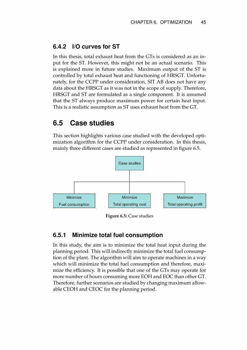
6.5 Case studies
This section highlights various case studied with the developed opti-mization algorithm for the CCPP under consideration. In this thesis,mainly three different cases are studied as represented in figure 6.5.
Figure 6.5: Case studies
6.5.1 Minimize total fuel consumption
In this study, the aim is to minimize the total heat input during theplanning period. This will indirectly minimize the total fuel consump-tion of the plant. The algorithm will aim to operate machines in a waywhich will minimize the total fuel consumption and therefore, maxi-mize the efficiency. It is possible that one of the GTs may operate formore number of hours consuming more EOH and EOC than other GT.Therefore, further scenarios are studied by changing maximum allow-able CEOH and CEOC for the planning period.

46 CHAPTER 6. OPTIMIZATION
6.5.2 Minimize total operating cost
In this study, the aim is to minimize the total operating cost of theCCPP under consideration. Total operating cost includes cost relatedto fuel consumption and EOH. Cost related to EOH represents the costof maintenance. Start-up cost for the GT is not considered as the start-up time of GT is less and hence, fuel consumption during the start-up is negligible compared to the fuel consumption during the oper-ation. Furthermore, sensitivity analysis is performed to evaluate anychange in operating pattern with change in cost associated with EOHand EOC. The results of fuel consumption during the planning periodare compared.
6.5.3 Maximize total operating profit
In this study, the aim is to maximize the profit of the plant under con-sideration. Revenue generated by selling the electricity and cost re-lated to Energy Not Served (ENS) are added to the objective function.
All of the studies are performed for one week and one month ofplanning period. In some cases, studies are also performed for differ-ent planning period where ambient conditions are varying.
6.6 Optimization problem
This section gives an idea about optimization model developed for thisthesis. The core of this algorithm is formulated by one of the ongoingthesis [15] at SIT AB. However, [15] does not include any constraintsregarding EOH and EOC. The objective of [15] is to minimize the totalfuel consumption of a CCPP under consideration.
IndicesIndices for the GT (i):GT01: 1, GT02:2Indices for the ST (j):ST: 1
Input parametersCITi,t = Compressor inlet temperature for machine i at time tRHi,t = Relative humidity for machine i at time t

CHAPTER 6. OPTIMIZATION 47
M InHeatpi
, IInHeati = Slope and intercept to estimate heat input for ma-
chine i, p = 1, 2, 3, 4MExHeat
pi, IExHeat
i = Slope and intercept to estimate exhaust for machinei, p = 1, 2, 3
Cai,t = Factor Ca for machine i at time t = Ca1 (From meta-models)Cbi,t = Factor Cb for machine i at time t = Cb1 (It is assumed that the GToperates with the gas fuel)Cci,t = Factor Cc for machine i at time t = Cc2 (This is more conservativeapproach)
MCEOHi = Maximum cumulative EOH for machine i during the plan-ning periodMCEOCi = Maximum cumulative EOC for machine i during the plan-ning period
λelt = Electricity price at time tλflt = Fuel price at time tOCEOHi = Cost per EOH for machine iDemandt = Total electricity demand at time t
Li,t = Minimum generation level for machine i at time tUi,t = Maximum available capacity for machine i at time t
T upi = Minimum up time for machine iT downi = Minimum down time for machine iT upj = Minimum up time for machine jT downj = Minimum down time for machine j
hON0i
= Number of planning periods since the machine i is ’ON’ at thebeginning of the planning periodhOFF0i
= Number of planning periods since the machine i is ’OFF’ at thebeginning of the planning periodu0i = Unit-commitment variable for machine i before starting of theplanning period
hON0j
= Number of planning periods since the machine j is ’ON’ at thebeginning of the planning period

48 CHAPTER 6. OPTIMIZATION
hOFF0j
= Number of planning periods since the machine j is ’OFF’ at thebeginning of the planning periodu0j = Unit-commitment variable for machine j before starting of theplanning period
Optimization variablesPi,t = Power output of machine i at time tPj,t = Power output of machine j at time t
hONi,t = ’ON’ time for machine i at time thOFFi,t = ’OFF’ time for machine i at time thONj,t = ’ON’ time for machine j at time thOFFj,t = ’OFF’ time for machine j at time t
ui,t = Unit-commitment variable for machine i at time tuj,t = Unit-commitment variable for machine j at time tsui,t = Starting-up variable for machine j at time t
Fueli,t = Fuel consumption of machine i at time tEOHi,t = EOH consumed of machine i at time tEOCi,t = EOC consumed of machine i at time t
ηj = Maximum efficiency of machine j
Optimization variables limitsui,t ∈ {0,1}uj,t ∈ {0,1}suj,t ∈ {0,1}
Pi,t ∈ Non Negative RealsPj,t ∈ Non Negative RealsEOHi,t ∈ Non Negative RealsEOCi,t ∈ Non Negative Reals
hONi,t ∈ Non Negative IntegershONj,t ∈ Non Negative IntegershOFFi,t ∈ Non Negative IntegershOFFj,t ∈ Non Negative Integers

CHAPTER 6. OPTIMIZATION 49
Constraints for the GTGeneration limit constraint
Li,t ∗ ui,t ≤ Pi,t ≤ Ui,t ∗ ui,t,Where, i = 1, 2; t = 1, 2, 3, ..., T (6.1)
Constraint on EOH
T∑t=1
EOHi,t ≤MCEOHi,Where, i = 1, 2 (6.2)
Constraint on EOC
T∑t=1
EOCi,t ≤MCEOCi,Where, i = 1, 2 (6.3)
Constraint for minimum up timeFor t = 1
hON0i≥ ui,t ∗ T up
i ,Where, i = 1, 2; t = 1, 2, 3, ..., T (6.4)
For t 6= 1
hONi,t ≥ ui,t−1 ∗ T up
i ,Where, i = 1, 2; t = 1, 2, 3, ..., T (6.5)
Constraint for minimum down timeFor t = 1
hOFF0i
+ u0i ∗ T downi ≥ T down
i ,Where, i = 1, 2; t = 1, 2, 3, ..., T (6.6)
For t 6= 1
hOFFi,t−1 + ui,t−1 ∗ T down
i ≥ T downi ,Where, i = 1, 2; t = 1, 2, 3, ..., T (6.7)
Constraints for the ST

50 CHAPTER 6. OPTIMIZATION
Generation limit constraint
Pj,t ≤2∑
i=1
ExHeati,t ∗ ui,t ∗ ηj,Where, j = 1; t = 1, 2, 3, ..., T (6.8)
Where,
ExHeati,t = (MExHeatp1
∗CITi,t)+(MExHeatp2
∗RHi,t)+(MExHeatp3
∗Pi,t)+IExHeati
(6.9)
In addition to constraint 6.8, power output limit of a ST depending onthe operating phase. If the ST can not produce maximum power if it isjust started. Therefore, different start-ups (cold, warm, hot) are mod-elled by [15]. These start-ups are modeled based on ST’s ’OFF’ time.Load balance constraint
2∑i=1
Pi,t +∑j=1
Pj,t = Demandt,Where, t = 1, 2, 3, ..., T (6.10)
Objective functionMinimize total fuel consumption
Minimize :T∑t=1
2∑i=1
Fueli,t (6.11)
Where,
Fueli,t = (M InHeatp1
∗CITi,t)+(M InHeatp2
∗RHi,t)+(M InHeatp3
∗Pi,t)+(M InHeatp3
∗P 2i,t)+I
InHeati
(6.12)
Minimize total operation cost
Minimize :T∑t=1
2∑i=1
(Fueli,t ∗ λflt + EOHi,t ∗OCEOHi) (6.13)
Maximize total profit
Maximize :T∑t=1
2∑i=1
Pi,t∗λelt−(Fueli,t∗λflt+EOHi,t∗OCEOHi)+T∑t=1
∑j=1
Pj,t∗λelt
(6.14)

CHAPTER 6. OPTIMIZATION 51
6.7 Optimization solver
This section gives brief idea of solver used to solve the formulated op-timization problem. For this thesis, academic version of IBM’s CPLEXsolver is used. CPLEX is a high-performance mathematical program-ming solver for linear, mixed-integer, and quadratic programming.Quadratic program is used when optimization constraints are linearbut objective function includes quadratic term [16]. Here MILP is for-mulated as the variable representing the square of power output islinearized.
6.7.1 Optimality tolerance
Sometimes CPLEX finds a good integer solution earl. However, it mustexamine additional nodes to prove that the solution is optimal. Thisconsumes additional computational power. However, user can speed-up the process by setting the optimality tolerance. CPLEX supportstwo type of solvers. Relative optimality tolerance guarantees that asolution lies within a certain percentage of the optimal solution. Ab-solute optimality tolerance guarantees that a solution lies within a cer-tain range of the optimal solution. According to [17], the default valueof the relative MIP gap tolerance is 1e-4; the default value of the abso-lute MIP gap tolerance is 1e-6. These default values indicate to CPLEXto stop when an integer feasible solution has been proved to be within0.01% of optimality. On a difficult model with input data obtainedwith only approximate accuracy, where a proved optimum is thoughtto be unlikely within a reasonable amount of computation time, a usermight choose a larger relative MIP gap to allow early termination; forexample, a relative MIP gap of 0.05 (corresponding to 5%). Conversely,in a model where the objective function amounts to billions of dollarsand the data are accurate to a degree that further processing is worth-while, a tighter relative MIP Gap (even 0.0) may be advantageous toavoid any chance of missing the best possible solution.

52 CHAPTER 6. OPTIMIZATION
6.7.2 Warm start
CPLEX has a provision to supply hints to help CPLEX find an initialsolution of MILP. This is referred as a MIP start, an advanced start, ora warm start. A MIP start might come from a different problem whichis previously solved or from knowledge of the problem [18]. A MIPstart may include continuous variables and discrete variables of vari-ous types, such as integer variables, binary variables, semi-continuousvariables, semi-integer variables, or variables appearing in special or-dered sets [18]. In this thesis, the optimization algorithm is imple-mented on a historical data of the CCPP under consideration. There-fore, historical value of output power and unit-commitment variableat for each planning interval is available. These values are supplied toCPLEX for solving the optimization problem. Problem may fail to doa warm start if the provided solution violates any optimization con-straints. As EOH and EOC are dependent on the unit-commitmentvariables, problem may fail to warm start depending on the constraintset for maximum CEOH and CEOC during the planning period.

Chapter 7
Results
This chapter discusses about the result obtained for the case studiesdefined in chapter 6. Optimization problem is solved for one week andone month period. Various scenarios are defined by varying maximumCEOH, maximum CEOC, and MipGap. Scenarios highlighted in bluerepresent the results for one month of operation planning. They arelimited due to increased computation start when the problem fail todo a warm-start. Results are plotted for highlighted scenarios. Resultof power output of GTs and ST are normalize. Furthermore, input dataof Compressor Inlet Temperature (CIT) is also normalized.
7.1 Minimize total fuel consumption
Table 7.1 summarizes the results for the case where objective is to min-imize the total fuel consumption of CCPP under consideration.
Figure 7.1 and figure 7.2 represents results for planning period of1 week in month 1. Limit on maximum CEOH and CEOC is set to ahigh value to develop a base case. However, MipGap set for these twoscenarios is different. It is interesting to observe that when MipGapis set to 2.5%, total consumed EOH and EOC are less compared to thescenario when MipGap is set to 0%. S3 gives lowest value of objectivefunction but it consumes highest number of EOH and EOC for oneweek. This is because of more switching operations. Furthermore,GT02 is utilized more. This leads to a conclusion that set accuracy tosolve the optimization problem has influence on consumption of EOHand EOC. It also takes more time to solve the problem.
Figure 7.3 represents the results for planning period of 1 week in
53

54 CHAPTER 7. RESULTS
Sr CEOH CEOC Warm MipGap Time Objective CEOH CEOCNo GT01 GT02 GT01 GT02 (Y/N) (%) (s) Function (MWh) GT01 GT02 GT01 GT02S1 1,000 1,000 50 50 Y 2.5 79.93 91,012.23 202.11 120.25 7.273 8.900S2 1,000 1,000 50 50 Y 1.0 173.99 89,988.39 208.00 264.50 23.000 23.250S3 1,000 1,000 50 50 Y 0.0 265.394 89,987.57 208.00 264.50 23.000 23.250S4 180 1,000 9 50 Y 1.0 104.471 91,018.32 173.00 84.37 1.000 2.225S5 160 1,000 8 50 N 2.5 792.619 91,076.25 156.86 285.25 7.273 31.150S6 160 250 8 12.5 N 2.5 508.682 90,896.91 155.86 187.62 7.273 12.125S7 160 160 8 8 N 2.5 1473.226 90,779.76 159.61 159.63 6.270 7.680S8 1,000 1,000 50 50 Y 2.5 752.980 308,279.16 706.860 119.250 7.270 8.900S9 1,000 1,000 50 50 Y 0.0 85.243 120,288.21 173.00 173.00 1.000 1.000S10 170 200 8.5 10 N 2.5 - Can’t solve - - - -S11 1,000 1,000 50 50 Y 2.5 655.448 469,289.76 677.00 677.00 1.000 1.000S12 1,000 650 50 32.5 N 2.5 - Can’t solve - - - -
Table 7.1: Summary of results (minimize total fuel consumption)
month 1. Limit on maximum CEOH and CEOC is reduced. Resultsshow that problem could not warm start and hence, solving time isvery high.
Figure 7.4 represents the results for planning period of a month.Limit on maximum CEOH and CEOC is set to a high value to developa base case. It is evident that GT01 is operated more compared to GT02.This is because of higher value of CIT for GT02. Efficiency of a GT isless when CIT is high and hence, the GT consumes more fuel, if oper-ated. Efforts were made to change the limit on maximum CEOH andCEOC so that both of the GTs can utilize equally. However, problemcould not warm start and expected solving time was enormous. Theseresults of scenarios S1 - S8 indicate the presence of chiller. Chiller isused to reduce CIT so that the GTs can be operated at higher effi-ciency. When the chiller is operating, CIT is lower. This also resultsinto higher maximum available capacity. GT02 stopped generating assoon as its CIT (input value) started increasing. Chiller also consumessome power and hence, total auxiliary consumption of plant increaseswhen the chiller is functional.
In order to check the effectiveness of the algorithm, another timeperiod was selected when CIT of both of the GTs is quite similar i.e.either chillers are operating or they are off for both of the GTs.
Figure 7.5 and figure 7.6 represents the results for planning periodin second month. The CIT for both of the GTs is almost identical. Re-sults show that GTs are consuming equal EOH and EOC. Furthermore,GT02 is operating near its maximum available capacity. When limit on

CHAPTER 7. RESULTS 55
maximum allowed EOH and EOC is reduced, problem failed to solve.It is interesting to observe that there is only one start-up, which hap-pens at the beginning of the the planning period. Therefore, consumedEOH is mainly because of total operating hours. If PPO aims to reduceconsumed EOH for any machine, PPO must turn off the machine. Itwas observed that the total demand faced by the CCPP was high dur-ing this time. Therefore, it is not feasible to meet total demand if anymachine is turned off. When any GT is turned off, output of ST willalso reduce because of reduction in total exhaust heat from the GTs.For such scenario, there should be a provision to drop fraction of de-mand i.e. ENS. However, PPO must consider additional cost for ENS.
Results show that overall plant efficiency is improved. However,now GT01 operating at lower efficiency while GT02 operating at higherefficiency compared to their historical efficiency measurements. Thisis rational as GT01 is generating less power while GT02 is generatingmore power compared to its historical active load measurement.
7.2 Minimize total operating cost
Table 7.2 summarizes the results for the case where objective is to min-imize the total operating cost of the CCPP under consideration. Timeseries of the fuel price and cost per EOH are given as the inputs to theoptimization problem. No cost is added for EOC as EOH and EOCare related. This cost is derived from the cost of maintenance contractsfor a GT during its life. Furthermore, this cost is normalized in orderto maintain the confidentiality. This cost is also varied to observe itseffect on the dispatch results, EOH and EOC consumption during theplanning period.
Sr CEOH CEOC Cost MipGap Time Fuel CEOH CEOCNo GT01 GT02 GT01 GT02 p.u/EOH (%) (s) (MWh) GT01 GT02 GT01 GT02S13 1,000 1,000 50 50 1.0 0.0 79.93 90,995.49 173.00 84.375 1.000 3.225S14 1,000 1,000 50 50 0.1 0.0 437.03 90,030.70 148.023 184.875 10.455 7.675S15 160 160 8 8 1.0 2.5 166.282 90,968.75 155.695 144.250 5.182 5.450S16 1,000 1,000 50 50 1.0 2.5 1,314.19 308,268.16 677.000 84.375 1.000 3.225S17 1,000 1,000 50 50 1.0 0.0 86.92 120,286.03 173.000 173.000 1.000 1.000S18 1,000 1,000 50 50 0.1 0.0 88.16 120,286.03 173.000 173.000 1.000 1.000S19 1,000 1,000 50 50 1.0 2.5 757.26 469,081.85 677.000 677.000 1.000 1.000
Table 7.2: Summary of results (minimize total operating cost)

56 CHAPTER 7. RESULTS
Figure 7.7 represents results for planning period of 1 week in month1 (S13). The cost/EOH is set to 1 p.u. Comparing these results withfigure 7.2, it is evident that the GT02 is not operating once it is shut-down. Total EOH consumption in this scenario is 257.375 comparedto 472.50 in S3. Total EOC consumption in this scenario is 3.225 com-pared to 46.250 in S3. However, the fuel consumption is increased by1.107%.
Figure 7.8 represents results for planning period of 1 week in month1 (S14). The cost/EOH is set to 0.1 p.u. Total EOH consumption in thisscenario is 332.898 compared to 472.50 in S3. Total EOC consumptionin this scenario is 18.130 compared to 46.250 in S3. These values arecertainly higher than that of obtained in S13. The fuel consumption isincreased by 0.04%.
The objective of the previous case study is to minimize the fuel con-sumption while satisfying the demand. Therefore, at any point in time,the GT with higher efficiency is operated and hence, more cycling isis observed. This is inference is backed by higher number of EOHand EOC consumed for this study. However, when the cost associatedis with EOH is included in the optimization problem, the situationchanges. It is a trade-off between increased cost of fuel consumptionversus the cost related to EOH. This is evident from the result of S13and S14. When the cost associated with EOH is less, more EOH andEOC are consumed. However, the fuel consumption is lesser.
Similar trends in EOH and EOC can be noticed in S15 and S16 aswell. For the second month, the results (S9 & S17, S12 & S19) are al-most identical. This is because the GTs are running during the wholeplanning period to satisfy the demand. Therefore, any cost related toEOH will not change the dispatch. This is evident from the results ofS9, S17, and S18. This might not have been the scenario if it is allowedto not serve the demand.
7.3 Maximize total operating profit
The objective of this case study is to maximize the profit of the CCPPunder consideration. Time series of the day ahead electricity price isgiven as an input to the optimization problem. Furthermore, it is al-lowed to drop the demand in order to satisfy the constraints on EOHand EOC, if required. Without the provision of energy not served, the

CHAPTER 7. RESULTS 57
optimization results are likely to be the same as maximize the operat-ing profit is equivalent to minimizing the operating cost as no otheroperating markets are considered.
The load balance constraint is represented in equation 7.1 whenENS is added. This is an additional variable in the optimization prob-lem.
2∑i=1
Pi,t +∑j=1
Pj,t = Demandt − ENSt,Where, t = 1, 2, 3, ..., T (7.1)
The objective function is represented in equation 7.2
T∑t=1
2∑i=1
(Pi,t−ENSt)∗λelt−(Fueli,t∗λflt+EOHi,t∗OCEOHi)+T∑t=1
∑j=1
Pj,t∗λelt
(7.2)
The load balance constraint and objective function can be formu-lated without increasing number of variables. This is represented inequation 7.3 and 7.4 respectively.
2∑i=1
Pi,t +∑j=1
Pj,t ≤ Demandt,Where, t = 1, 2, 3, ..., T (7.3)
T∑t=1
2∑i=1
(2Pi,t−Demandt)∗λelt−(Fueli,t∗λflt+EOHi,t∗OCEOHi)+T∑t=1
∑j=1
2∗Pj,t∗λelt
(7.4)
After inclusion of ENS, computation time increased exorbitantly.Therefore, it was not feasible to get the results for planning periodone week and one month and hence, more efficient approaches formodelling is envisaged. However, it could not be implemented heredue to time limitations. Furthermore, penalty for ENS is consider sameas the electricity price for simulation purpose.

58 CHAPTER 7. RESULTS
Figure 7.1: Results: S1, week - 1, month - 1

CHAPTER 7. RESULTS 59
Figure 7.2: Results: S3, week - 1, month - 1

60 CHAPTER 7. RESULTS
Figure 7.3: Results: S7, week - 1, month - 1

CHAPTER 7. RESULTS 61
Figure 7.4: Results: S8, month - 1

62 CHAPTER 7. RESULTS
Figure 7.5: Results: S9, week - 1, month - 2

CHAPTER 7. RESULTS 63
Figure 7.6: Results: S9, month - 2

64 CHAPTER 7. RESULTS
Figure 7.7: Results: S13 (cost/EOH = 1.0 pu), week - 1, month - 1

CHAPTER 7. RESULTS 65
Figure 7.8: Results: S14 (cost/EOH = 0.1 pu), week - 1, month - 1

Chapter 8
Conclusion and Further Studies
• Meta-models developed to estimate TIT and TET provides rea-sonable accuracy to compute EOH and EOC. However, it wasfound that the CCPP under consideration does not have any his-tory of peaking operation. It is envisaged to carry out the sim-ilar studies on a power plant that performs peaking operations.This will allow to make more exhaustive meta models. GT canproduce more power than its maximum available capacity whiledoing a peaking operation. Therefore, innovative method to for-mulate generation limit constraint is envisaged to allow peakingoperation, whenever it is beneficial.
• It is envisaged to perform the studies on a CCPP that has morethan one block to estimate computational cost and robustness ofthe model.
• Results of optimization problem shows potential savings and in-crease in the profit over the planning interval. However, there isa possibility to add more components in the optimization prob-lem to achieve more accurate results. Furthermore, computationtime represents the bottleneck without a warm start. As the prob-lem uses historical data, warm start is feasible. However, forthe planning of future operation with the forecasted data, twostage optimization is envisaged where in first stage the problemis solved without inclusion of the constraints on EOH and EOC.This set of solution shall be used to do the warm start.
• In this thesis E[Cd] is used when there is any shutdown. In realitymost of the shutdown events are likely to be a normal shutdown
66

CHAPTER 8. CONCLUSION AND FURTHER STUDIES 67
and hence, Cd1 will be used to estimate the EOC during the shut-down. However, E[Cd] > Cd1 therefore, the algorithm will con-sume more number of EOC than the GT would have consumedin reality. One possible solution to rectify this, is to useCd1 for ev-ery shutdown and then apply some corrective maintenance costfor UL1, UL2, and UL3 events.
• In this thesis exhaust heat of the the GTs is added to determinethe power output of the ST. However, in reality it depends onthe plant’s configuration. Exhaust heat is lower when the GT isoperating on partial load. Suppose, one GT is operating at par-tial load and one GT is operating at full load. If the CCPP has acommon HRSGT then it will not be efficient to mix the exhaustof both GTs as it will reduce overall temperature of the exhaustgas. If the CCPP has seperate HRSGT then it will take more timeto achieve the steam parameter for the HRSGT that receives ex-haust from the GT which is running at partial load. Furthermore,there can be a provision for auxiliary firing in the HRSGT. There-fore, it is essential to know detailed configuration of the CCPPto formulate additional constraints. Otherwise, the results arelikely to overestimate the efficiency.
• From the data of CIT for the planning period of one week, it isevident that the CCPP has a chiller. CCPP turned off the chillerof GT02 as GT02 stopped producing. Historical data that also in-clude CIT is used in this thesis. However, when historical dataof CIT is used, it indicates that CIT for GT02 is high so it is notefficient to operate that machine. It might be possible to get evenbetter result if GT02 is operating with the chiller on. Therefore,it is essential to model the chiller and use the data of ambienttemperature to get the optimum results. However, for this pur-pose additional data like power consumption of chiller is alsorequired. Such inclusion is likely to increase the accuracy of theresults but it will also increase the computation cost and time dueto increased number of variables.
• In order to get rational results, time period when the chillers ofboth GTs are operating, was selected. Results shows improve-ment in overall plant’s efficiency. The way overall efficiency ismodeled, absence of chiller’s model will not affect the results.

68 CHAPTER 8. CONCLUSION AND FURTHER STUDIES
However, it will certainly have effect on total operating cost andprofit of the CCPP due to some power consumption by the chiller.This also reflects the need of including auxiliary power consump-tion of the CCPP under consideration.
• In this thesis, the cost associated with EOH and EOC is computedbased on total cost of maintenance contract during the life of theGT. Throughout the life of the machine, several types of mainte-nance are scheduled. Their cost and time to perform the mainte-nance are varying. It is also possible to model the maintenanceevent. Such approach will be give more realistic results as it willalso consider the loss of revenue during the maintenance period.However, a major challenge is that the maintenance intervals areoften longer. This means that the length of planning period willincrease. This will increase computational time and cost. Fur-thermore, the accuracy in long-term forecast of electricity andfuel price represents the bottleneck for having longer planningperiod.
• The cost associated with EOH and EOC is only valid for the ma-chine which is not operating in cyclic regime i.e. at any point intime total consumed EOC shall be less than or equal to the spec-ified EOC for respective value of EOH. Therefore, it is envisagedto perform the similar studies for the CCPP that operates in cyclicregime.

Bibliography
[1] W. Watson, “The success of the combined cycle gas turbine”, inInternational Conference on opportunities and advances in Interna-tional power generation, 1996, pp. 87–92.
[2] U. Colpier and D. Cornland, “The economics of the combinedcycle gas turbine - an experience curve analysis”, pp. 309–316,2002.
[3] ERG. (). How a combined cycle plant works, [Online]. Avail-able: https://www.erg.eu/en/our-energy/natural-gas/how-a-combined-cycle-plant-works (visited on07/13/2019).
[4] E. Lobato, P. Sánchez-Martín, and E. Sáiz-Marín, “Long termmaintenance optimization of ccgt plants”, 2012.
[5] O. Anubi, A. Menon, and A. Kumar, “Gas turbine dispatch opti-mizer”, U.S. Patent : 15 / 476 , 084, Mar. 31, 2017.
[6] M. Gröger, “Models and methods for reliability based mainte-nance scheduling”, PhD thesis, Universität Wuppertal, 2016.
[7] M. Aganagic, J. G. Frame, and D. Hadziosmanovic, “Systems,methods and apparatus for integrated optimal outage coordi-nation in energy delivery system”, U.S. Patent : 14 / 624 , 681,Feb. 18, 2015.
[8] P. Rodilla, S. Cerisola, and C. Batlle, “Modeling the major over-haul cost of gas-fired plants in the unit commitment problem”,2014.
[9] S. Wogrin, D. Galbally, and A. Ramos, “Ccgt unit commitmentmodel with first-principle formulation of cycling costs due to fa-tigue damage”, Energy, vol. 113, pp. 227–247, 2016.
69

70 BIBLIOGRAPHY
[10] N. Troy, D. Flynn, M. Milligan, and M. O’Mally, “Unit commit-ment with dynamic cycling cost”, 2012.
[11] C. Assémat, Management of thermal power plants through use val-ues, 2015.
[12] J. Alemany, D. Moitre, and H. Pinto, “Short-term scheduling ofcombined cycle units using mixed integer linear programmingsolution”, 2013.
[13] F. J. Heredia, M. J. Rider, and C. Corchero, “A stochastic pro-gramming model for optimal electricity market bid problem withbilateral contracts for thermal and combined cycle units”, 2013.
[14] C. Liu, M. Shahidehpour, Z. Li, and M. Fotuhi-Firuzabad, “Com-ponent and mode models for the short-term scheduling of com-bined -cycle units”, 2009.
[15] S. Rosso, “Economic dispatch of combined cycle power plantsusing machine learning”, unpublished master thesis, 2019.
[16] IBM. (). Solving problems with a quadratic objective (qp), [On-line]. Available: https://www.ibm.com/support/knowledgecenter/SSSA5P_12.8.0/ilog.odms.cplex.help/CPLEX/UsrMan/topics/cont_optim/qp/01_QP_title_synopsis.html(visited on 08/11/2019).
[17] ——, (). Terminating mip optimization, [Online]. Available: https://www.ibm.com/support/knowledgecenter/SSSA5P_12.6.2/ilog.odms.cplex.help/CPLEX/UsrMan/topics/discr_optim/mip/usage/11_terminate.html (visitedon 08/11/2019).
[18] ——, (). Starting from a solution: Mip starts, [Online]. Available:https://www.ibm.com/support/knowledgecenter/SSSA5P_12.6.2/ilog.odms.cplex.help/CPLEX/UsrMan/topics/discr_optim/mip/para/49_mipStarts.html(visited on 08/11/2019).
[19] S. Swaminathan. (2018). Linear regression—detailed view, [On-line]. Available: https://towardsdatascience.com/linear-regression-detailed-view-ea73175f6e86 (visited on07/10/2019).

BIBLIOGRAPHY 71
[20] O. Botvinnik. (). Linear regression—detailed view, [Online]. Avail-able: https://olgabotvinnik.com/blog/logistic-regression-tutorial/ (visited on 07/11/2019).
[21] H. Krishni. (2018). K-fold cross validation, [Online]. Available:https://medium.com/datadriveninvestor/k-fold-cross-validation-6b8518070833 (visited on 07/08/2019).
[22] M. Sanjay. (2018). Why and how to cross validate a model?, [On-line]. Available: https://towardsdatascience.com/why-and-how-to-cross-validate-a-model-d6424b45261f(visited on 07/08/2019).
[23] K. Vinay. (2018). Why and how to cross validate a model?, [On-line]. Available: https://www.datascience.com/blog/imbalanced-data (visited on 07/09/2019).
[24] W. E. Hart, C. D. Laird, J.-P. Watson, D. L. Woodruff, G. A. Hacke-beil, B. L. Nicholson, and J. D. Siirola, Pyomo - Optimization Mod-eling in Python, Second Edition. Springer International Publishing,2012.

Part I
Appendix
72

Appendix A
Linear regression
Linear regression is one of the machine learning techniques that isused for determining linear relationship between target and one ormore target predictors.
A.1 Simple linear regression
Simple linear regression is useful for finding relationship between twocontinuous variables. One is predictor or independent variable andother is response or dependent variable. More than one predictors canalso be used to predict a dependent variable. It is refereed as multiplelinear regression.
Linear regression looks for statistical relationship but not determin-istic relationship. Relationship between two variables is said to be de-terministic if one variable can be accurately expressed by the other.For example, using temperature in degree Celsius it is possible to ac-curately predict Fahrenheit. Statistical relationship is not accurate indetermining relationship between two variables. For example, rela-tionship between height and weight. [19]
In this thesis piecewise linear regression is used to develop themeta-models while multiple linear regression is used to estimate heatinput and exhaust heat. The parameters used for this purpose is strictlyconfidential. However, correlation matrix was formed to select suit-able parameters to perform the regression. This section explains sim-ple mathematics behind the linear regression.
Let, ’y’ be a variable of interest, dependent on independent variable’x’. With simple linear regression, linear relationship between ’y’ and
73

74 APPENDIX A. LINEAR REGRESSION
’x’ is established as represented in equation A.1. It is possible thatvariable ’x’ can be non-linear. It can take any shape for example, it canbe ’x2’ as well. In that case, linear relationship between ’y’ and ’x2’ canbe established using the simple linear regression.
yi = f(xi) = β1 ∗ xi + β0 + ε (A.1)
Where,yi = Estimated value of ’y’ using simple linear regressionxi = Independent variabley = True value of variable of interestβ0 and β1 = Regression coefficientsε = Random error with E[ε] = 0
This equation represents the equation of line (y = m*x + c) where,β1 is the slope (m) and β0 is the intercept (c).
Values of β0 and β1 are determined by the regression algorithm insuch a way that the sum of squared error is represented in equationA.2 minimized. Once the values of β0 and β1 are estimated, best fittedline can be piloted as shown in figure A.1 and figure 4.12. Distancebetween data points and best fitted line is called residue.
Error =n∑
i=1
(y − yi)2 =n∑
i=1
(y − β1 ∗ xi − β0)2 (A.2)
If more than one predictor is used to estimate the value of ’y’, β canbe obtained as shown in equation A.3 [19]. To compute the inverse ofXTX , it is essential to have this matrix to be of full rank else it wouldresult in singular matrix which is not inevitable. Therefore, it is impor-tant to select the predictors that are not co-linear. This can be checkedby formulating the correlation matrix.
β = (XTX)−1XTy (A.3)
Where,y = True value of variable of interestβ = Vector representing regression coefficients

APPENDIX A. LINEAR REGRESSION 75
Figure A.1: Best fitted line [20]
X = Vector representing predictors
A.2 K-fold cross verification
Sometimes, evaluating a machine learning model can be challenging.As highlighted in A.1, the data set is divided into training and testdata set randomly. The model performance is evaluated by the errormetric. However, this might not be so reliable as training and test datais selected randomly. Therefore, it is possible that the trained modelmay give large error when tested using the test data. This is evident

76 APPENDIX A. LINEAR REGRESSION
from the results represented in figure 4.5 and figure 4.11.K-fold cross validation addresses this challenge by dividing the
data into folds and ensuring that each fold is used as a testing set [21].Let us assume that the available data is divided in K number of folds.In first iteration, the first fold is used to test the data while others formthe training data. In second iteration, the second fold is used to testthe data while others form the training data. This process is repeatedfor all K number of folds. This is represented in A.2. Results obtainedusing K-fold cross validation are less biased compare to random splitapproach as it ensures that every observation from the original dataset has the chance of appearing in training and test set.[22]
Figure A.2: K-fold cross validation
However, K-fold cross validation is not implemented in this thesisproject. As noticed from chapter4, piecewise linear regression is usedto establish the relationship between the variable of interest. There-fore, K-fold cross validation needs to be performed for each piecewisestep. However, there are not sufficient data points for some sets andhence, it is not practical to implement the K-fold cross validation tech-nique. This problem is also referred as an imbalance data in the fieldof data science. More information about it is represented in the A.3
A.3 Imbalance in data set
In the case of the imbalanced data, majority classes dominate the mi-nority classes. This creates biased results as most machine learningalgorithms assumes that the data is equally distributed. This resultsin poor classification of minority class. For example, algorithm thatdetects the frauds will always have majority data points with nor-mal transactions and hence, the results are likely to be dominated by

APPENDIX A. LINEAR REGRESSION 77
normal transaction. This challenge can be addressed during the pre-processing stage by doing re-sampling. This includes oversampling orundersampling as shown in figure A.3.
Figure A.3: Re-sampling techniques [23]
Random undersampling is a method in which we randomly selectthe samples from the majority class and drop the remaining. This isa classical method in which the goal is to balance class distributionsthrough the random elimination of majority class examples. This leadsto discarding potentially useful data that could be important for clas-sifiers.
Oversampling aims to achieve an equal distribution by eliminatingmajority class samples, it does this by replicating the minority samplesso that the distribution is balanced. However, oversampling has a fewshortcomings. It increases the probability of over-fitting as it makesexact replications of the minority samples rather than sampling fromthe distribution of minority samples.
Though there are not so many data points for lower values of %load, re-sampling is not implemented. This is due to the fact that thegas turbines are rarely operated at such low level of power output andthe estimated values of TIT and TET are not affecting the accuracy inEOH and EOC calculation. Furthermore, there were no data points

78 APPENDIX A. LINEAR REGRESSION
presenting % load values above 100%. The behaviour of the gas tur-bine is likely to be different when % load is above 100%.

Appendix B
Pyomo
This appendix provides brief overview about Pyomo for understand-ing of the reader. Actual algorithm of the code is not included in thereport to maintain the secrecy. However, a relevant example is pre-sented so that readers can understand the formulation of optimizationproblem using Pyomo. Details mentioned here are extracted from [24].Reader is envisaged to go through it for deeper understanding of Py-omo.
B.1 Overview of Pyomo
This section gives overview about the components and modelling strate-gies of Pyomo. It also discusses about the concept of concrete and ab-stract models. Pyomo supports an object-oriented design for definingoptimization models.
B.1.1 Abstract and concrete Models
Pyomo supports concrete models and abstract models for model dec-laration. In abstract model, model is declared first, and componentconstruction is delayed until the data is loaded and Pyomo creates themodel instance. This requires a two-pass approach where the model isdeclared in the first pass, and subsequently the model is constructedusing data values that are specified separately. The concrete model canbe used when data is available before model components are declared.Concrete models support a more programmatic style where the modelinstance is created immediately; model components are constructed
79

80 APPENDIX B. PYOMO
and initialized on the first pass as Python executes the model script.Model construction process is visualized in figure B.1. In this the-sis concrete model is implemented as the required data for the powerplant under consideration is available
Figure B.1: Model construction process [24]
B.1.2 Pyomo components
A Pyomo model object contains a collection of modeling componentsthat define the optimization problem. Some common modeling com-ponents supported by Pyomo are as below.
• Var: The Var component is used to represent the optimizationvariables in model. Variable component supports arguments todefine the domain and to initialize the variables, if required.
• Objective: It represents the objective function that needs to beminimized or maximized using the solver. B y default Pyomominimizes the objective function. For maximization problem, theflag to indicate the sense is changed.
• Constraints: It defines the constraints of the optimization prob-lem. This component contains expressions.
• Set: Set component is a collection of data. It is mainly used todefine indices for other components.

APPENDIX B. PYOMO 81
• Param: This component is used to represent numerical or sym-bolic values for data in the optimization problem.
B.2 Structured modeling with blocks
Pyomo allows to construct hierarchically structured models using ‘Block’component. Modeler can define fundamental building blocks, andthen construct the overall problem by connecting these blocks togetherin an object-oriented manner. ‘Block’ component can be treated as acontainer, consisting groups of variables and constraints. This conceptof modeling using ‘Block’ is illustrated using an example from powersystem studies.
Figure B.2: Multi-period planning problem [24]
Suppose, we are aiming to run some system studies for certain pe-riod. We can construct a block that consists the models of power sys-tem components. It is also possible to create a block for individualcomponent within the main block. Problem formulation with block isvery convenient for multiple time periods planning problems. Block iscalled at each time-stamp to perform the desired operation in this casesystem studies. This is represented in figure B.2

82 APPENDIX B. PYOMO
While discussing the block hierarchy, parent-child structure is fol-lowed. The root of the block hierarchy is always the current model.Furthermore, components and equation from anywhere within the hi-erarchy can be referenced. It is important to note that the componentnames must be unique within a single block. However, they do notneed to be unique globally. Block components can also be indexed ini-tialized using the construction rules highlighted in the previous sec-tion.
B.3 Generalized disjunctive programming
A common feature of many discrete optimization problem is the selec-tion among two or more mutually exclusive choices. Let us considerthe unit commitment problem for short-term planning operation of aCCPP. There are several constraints that depends on the current stateof operation. This is explained as below.
• There is a limit on minimum generation level when the machineis in ‘ON’ state. This limit is often not zero. However, when themachine is ‘OFF’ state, the power output must be zero.
• Change in output power at any time stamp must be within theramping limits. However, these limits are different when the ma-chine is in normal operation and when the machine is in start-upor shut-down phase.
• Gas turbines have short start-up time. However, it is not the casefor the steam turbines. Start-up of the steam turbine can be quick,or it can take time depending on the ‘off’ time. If it is a warmstart, then the ST can produce power quickly. If it is a cold-start,ST cannot deliver power immediately unless the steam parame-ters are achieved.
GDP is very effective to formulate models that are subjected tooperating state using ‘disjunction’. Each disjunction contains several‘disjunct’ connected by an ‘OR’ operator. Each disjunct represents dis-tinct operating state. These disjuncts are mutually exclusive.

APPENDIX B. PYOMO 83
B.4 Pyomo examples
B.4.1 The warehouse location problem
Problem: Let N be a set of candidate warehouse locations, and let Mbe a set of customer locations. For each warehouse n, the cost of deliv-ering product to customer m is given by dn,m. We wish to determinethe optimal warehouse locations that will minimize the total cost ofproduct delivery. The binary variables yn are used to define whetheror not a warehouse should be built, where yn is 1 if warehouse n isselected and 0 otherwise. The variable xn,m indicates the fraction ofdemand for customer m that is served by warehouse n. Furthermore,total number of warehouses that can be built is limited to P.
Given data:
Customer locations, M = [‘NYC’, ‘LA’, ‘Chicago’, ‘Houston’]
Warehouse locations, N = [‘Harlingen’, ‘Memphis’, ‘Ashland’]
Number of warehouse that can be built, P = 2
NYC LA Chicago Houston
Harlingen 1956 1606 1410 330Memphis 1096 1792 531 567Ashland 485 2322 324 1236
Table B.1: Cost of delivery from warehouse m to customer n
Optimization problem in words:

84 APPENDIX B. PYOMO
minimizex,y
∑n∈N
∑m∈M
xn,m ∗ dn,m
subject to ∑n∈N
xn,m = 1, ∀m ∈M
xn,m ≤ yn, ∀m ∈M, ∀n ∈ N∑n∈N
yn ≤ P
0 ≤ x ≤ 1
y ∈ {0, 1}
Solution using Pyomo:
Figure B.3 represents the formulation of the warehouse problem in Py-omo.First of all, Pyomo environment is imported as shown in line 2.
Line 4 creates a ConcreteModel and provides a name.
Line 6 to line 20 provide the input data for the optimization problem
Line 22 defines the variable x to represent the demand catered fromN warehouse to M customer location. This variable is indexed over Nand M. Furthermore, it is bounded between 0 and 1 as this variablerepresents the demand catered.
Line 23 defines the variable y to represent if the warehouse shall bebuilt in N or not and hence, it is a binary variable.
Line 25 to line 27 defines the objective function that is summed over Nand M using for command.
Line 29 to line 32 defines the constraint over the demand. It ensuresthat demand of each customer is fully met.
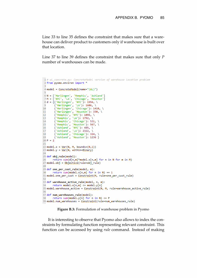
APPENDIX B. PYOMO 85
Line 33 to line 35 defines the constraint that makes sure that a ware-house can deliver product to customers only if warehouse is built overthat location.
Line 37 to line 39 defines the constraint that makes sure that only Pnumber of warehouses can be made.
Figure B.3: Formulation of warehouse problem in Pyomo
It is interesting to observe that Pyomo also allows to index the con-straints by formulating function representing relevant constraint. Thisfunction can be accessed by using rule command. Instead of making

86 APPENDIX B. PYOMO
function, user can also write individual constraints. However, it ismore tedious way. Furthermore, if user wants to change anything, userhas to make changes in all constraints. This is also prone to humanerrors. By defining constraints using function, it is very convenient tomake any changes in the constraint. It also make the algorithm cleaner.
B.4.2 Constraints formulation using disjuncts
Figure B.4 provides an idea about formulating constraints using dis-juncts. Disjuncts are used to model mutually exclusive states. This isoften the case for generation planning problem. For example, rampingrates are different for normal operating state, start-up, and shut-downstate. In a similar way, generation limits also varies for different states.
Line 8 to line 15 provides the input parameters regarding power limitsand ramp rates indexed over the set of generators.
Line 17 to line 19 define a variable that represents the power output,bounded between zero to the maximum power limit.
Line 21 to line 26 defines the constraints on the power limit and ramp-ing for the generators during ON state. The power limit is betweenminimum and maximum generation while the ramping limit is set tothe ramping rate during the normal operation
Line 30 to line 35 defines the constraints on the power limit and ramp-ing for the generators during OFF state. The power limit is set to bezero as the machine will not produce any power in this state. Theramping limit is set to the ramping rate during the shut-down opera-tion
Line 39 to line 43 defines the constraints on the power limit and ramp-ing for the generators during Start-up state. The power limit is set tobe between zero and ramping rate during start-up process.
Line 28, line 37, and line 43 define the mutually exclusive states as adisjunct for any generator at any time stamp. Line 48 connects all dis-juncts for any generator at any time stamp using rule = bindgenerators

APPENDIX B. PYOMO 87
Figure B.4: Constraint formulation using disjuncts in Pyomo

TRITA EECS-EX-2019:627
www.kth.se