Economic Feasibility of Electrochemical Caustic Recycling at the

PNNL-18265

Prepared for the U.S. Department of Energy under Contract DE-AC05-76RL01830

Economic Feasibility of Electrochemical Caustic Recycling at the Hanford Site AP Poloski GJ Sevigny DE Kurath MS Fountain LK Holton March 2009

PNNL-18265

Economic Feasibility of Electrochemical Caustic Recycling at the Hanford Site AP Poloski GJ Sevigny DE Kurath MS Fountain LK Holton March 2009 Prepared for the U.S. Department of Energy under Contract DE-AC05-76RL01830 Pacific Northwest National Laboratory Richland, Washington 99352

iii

Summary

This report contains a review of potential cost benefits of NaSICON Ceramic membranes for the separation of sodium from Hanford tank waste. The primary application is for caustic recycle to the Waste Treatment and Immobilization Plant (WTP) pretreatment leaching operation. The report includes a description of the waste, the benefits and costs for a caustic-recycle facility, and Monte Carlo results obtained from a model of these costs and benefits. The use of existing cost information has been limited to publicly available sources. This study is intended to be an initial evaluation of the economic feasibility of a caustic recycle facility based on NaSICON technology.

The current pretreatment flowsheet indicates that approximately 6,500 metric tons (MT) of Na will be added to the tank waste, primarily for removing Al from the high-level waste (HLW) sludge (Kirkbride et al. 2007). An assessment (Alexander et al. 2004) of the pretreatment flowsheet, equilibrium chemistry, and laboratory results indicates that the quantity of Na required for sludge leaching will increase by 6,000 to 12,000 MT in order to dissolve sufficient Al from the tank-waste sludge material to maintain the number of HLW canisters produced at 9,400 canisters as defined in the Office of River Protection (ORP) System Plan (Certa 2003). This additional Na will significantly increase the volume of LAW glass and extend the processing time of the Waste Treatment and Immobilization Plant (WTP). Future estimates on sodium requirements for caustic leaching are expected to significantly exceed the 12,000-MT value and approach 40,000-MT of total sodium addition for leaching (Gilbert, 2007).

The cost benefit for caustic recycling is assumed to consist of four major contributions: 1) the cost savings realized by not producing additional immobilized low-activity waste (ILAW) glass, 2) caustic recycle capital investment, 3) caustic recycle operating and maintenance costs, and 4) research and technology costs needed to deploy the technology. In estimating costs for each of these components, several parameters are used as inputs. Due to uncertainty in assuming a singular value for each of these parameters, a range of possible values is assumed. A Monte Carlo simulation is then performed where the range of these parameters is exercised, and the resulting range of cost benefits is determined.

The major conclusions from the Monte Carlo model results discussed in this report are summarized below:

• A feasible region for minimal plant economics (e.g; 10% total return on investment) corresponds to approximately 10,000 MT sodium recycled. Total return on investments in the range of 30-60% can be achieved when 50,000 MT of sodium are recycled.

• Literature data for the growth rate of Gibbsite particles indicates that particles forming in the 1- to 10-micron range over the average vessel residence time of 1 week corresponds to a saturation ratio less than eight. The operation of the downstream WTP processes under these conditions and with particles of this size must be demonstrated in a separate experimental program.

• Recycling 10,000 MT of sodium results in a cost savings in ILAW glass of $0.7B to $1.0B. If 30,000 MT of sodium is recycled, $2.5B to $3.1B would likely be realized.

• Recycling 10,000 MT of sodium results in an estimated range of total capital cost for the caustic-recycle facility to be $175M to $325M. If 30,000 MT of sodium is recycled, $200M to $350M would likely be realized.

iv

• Recycling 10,000 MT of sodium results in a total production cost for the caustic-recycle facility to be in the range of $13M/yr to $21M/yr. If 30,000 MT of sodium is recycled, $21M/yr to $30M/yr would likely be realized.

• If 10,000 MT of sodium is recycled, a specific production cost is estimated to be in the range of $25/kg to $45/kg. If 30,000 MT of sodium is recycled, $15/kg to $22/kg would likely be realized.

• The specific sales cost is invariant with the amount of sodium recycled. A specific sales cost is estimated to be in the range of $84/kg to $104/kg. The specific sales cost is a factor of 3.8 to 6.9 greater than the expected specific production cost range.

• An improved cost benefit analysis for caustic recycle facilities should focus on improving the basis for the following questions (listed in priority): How much sodium will be added for caustic leaching?

– What level of supersaturation can be tolerated?

– What is the cost savings from preventing additional ILAW glass production?

– What are the total capital costs for the caustic-recycle facility?

– What are the operating and maintenance costs for the caustic-recycle facility?

v

Acknowledgements

This analysis relied strongly on the elicitation of information and informed judgment from knowledgeable Department of Energy, Bechtel National Inc., Ceramatec Inc., and Pacific Northwest National Laboratory staff. Although this list is incomplete, the authors would like to acknowledge the following for their participation: Billie Mauss (DOE), Shekar Bologapal (Ceramatec Inc.), Anthony Nickens (Ceramatec Inc.).

vii

Acronyms and Abbreviations

ACE U.S. Army Corps of Engineers DOE Department of Energy HLW high-level waste ILAW immobilized low-activity waste LAW low-activity waste LLW low-level waste MT metric ton O&M operations and maintenance ORP Department of Energy-Office of River Protection PNNL Pacific Northwest National Laboratory ROI total return on investment R&T research and technology TWRS Tank Waste Remediation System WTP Waste Treatment and Immobilization Plant

ix

Contents

Summary ............................................................................................................................................... iii Acknowledgements ............................................................................................................................... v

Acronyms and Abbreviations ............................................................................................................... vii 1.0 Introduction .................................................................................................................................. 1.1

2.0 Scope and Objectives .................................................................................................................... 2.1

3.0 Methods ........................................................................................................................................ 3.1

3.1 WTP Pretreatment Stream Composition ............................................................................. 3.1

3.2 Sodium Removal ................................................................................................................. 3.4

3.3 Aluminum Solubility Model ............................................................................................... 3.5

3.4 ILAW Glass Model ............................................................................................................. 3.7

3.5 Delta ILAW ........................................................................................................................ 3.8

3.6 ILAW Cost Savings ............................................................................................................ 3.8

3.7 Estimated Membrane-Area Requirements .......................................................................... 3.9

3.8 Estimated Facility Size........................................................................................................ 3.10

3.9 LAW Vitrification Facility Costs ........................................................................................ 3.10

3.10 Estimated Capital Costs ...................................................................................................... 3.11

3.11 LAW Vitrification Labor Costs .......................................................................................... 3.11

3.12 Estimated Labor Costs ........................................................................................................ 3.12

3.13 Estimated Electrical Needs ................................................................................................. 3.13

3.14 Estimated Electrical Costs .................................................................................................. 3.13

3.15 Membrane-Replacement Frequency ................................................................................... 3.14

3.16 Membrane Replacement Costs............................................................................................ 3.14

3.17 Estimated Research and Technology Costs ........................................................................ 3.15

3.18 Estimated Total Capital Investment .................................................................................... 3.15

3.19 Estimated Operating and Maintenance Costs ..................................................................... 3.16

3.20 Estimated Cost Benefit........................................................................................................ 3.17

4.0 Results .......................................................................................................................................... 4.1

4.1 Return on Investment .......................................................................................................... 4.1

4.2 Cost Savings ........................................................................................................................ 4.5

4.3 Capital Costs ....................................................................................................................... 4.5

4.4 O&M Costs ......................................................................................................................... 4.5

4.5 Specific Sale and Production Costs .................................................................................... 4.6

4.6 Impact on Hanford Waste Processing ................................................................................. 4.7

4.7 Sensitivity Analysis ............................................................................................................ 4.8

5.0 Conclusions .................................................................................................................................. 5.1

6.0 References .................................................................................................................................... 6.1

x

Figures

3.1 Illustration of WTP Process Integration ...................................................................................... 3.1

3.2 Illustration of Possible WTP Process Integration Scheme .......................................................... 3.3

3.3 Schematic of a Two Compartment Electrochemical Process Using the NaSICON Membrane ................................................................................................................................... 3.4

3.4 Gibbsite Solubility – Molarity of Al in Solution for Given Initial Solution NaOH Molarity ..... 3.5

3.5 Saturation Ratio at 25ºC of Just Saturated Solutions at Elevated Temperatures......................... 3.6

3.6 Experimentally Measured Crystal Growth Rates of Saturated Sodium Aluminate Solutions at 22ºC ......................................................................................................................................... 3.7

3.7 Predicted Time Needed to Precipitate Gibbsite Particles of Various Sizes Under Different Saturation Ratio Conditions ........................................................................................................ 3.7

4.1 ROI for Various Amounts of Caustic Recycled .......................................................................... 4.1

4.2 Total Sodium Recycled with Varoius Amounts of Sodium Added for Leaching and Aluminate Saturation Temperatires for the Sodium-Recycled Product ...................................... 4.2

4.3 Sodium Aluminate Saturation Ratio as a Function of Saturation Temperature .......................... 4.3

4.4 Total Sodium Recycled with Various Amounts of Sodium Added for Leaching and Aluminate Saturation Temperatures for the Sodium-Recycled Product ..................................... 4.3

4.5 ROI as a Function of Aluminate Saturation Ratios with Various Amounts of Sodium Added for Caustic Leaching; top – 90%; middle – 50%; bottom 10% of Monte Carlo Realizations Below Each Curve ....................................................................................................................... 4.4

4.6 ILAW Net Cost Savings as a Function of Total Sodium Recycled ............................................ 4.5

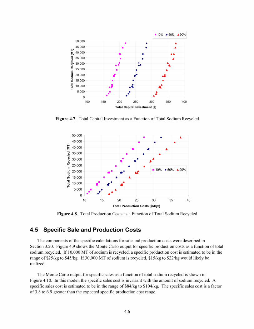
4.7 Total Capital Investment as a Function of Total Sodium Recycled ............................................ 4.6

4.8 Total Production Costs as a Function of Total Sodium Recycled ............................................... 4.6

4.9 Specific Production Costs as a Function of Total Sodium Recycled .......................................... 4.7

4.10 Specific Sales Costs as a Function of Total Sodium Recycled ................................................... 4.7

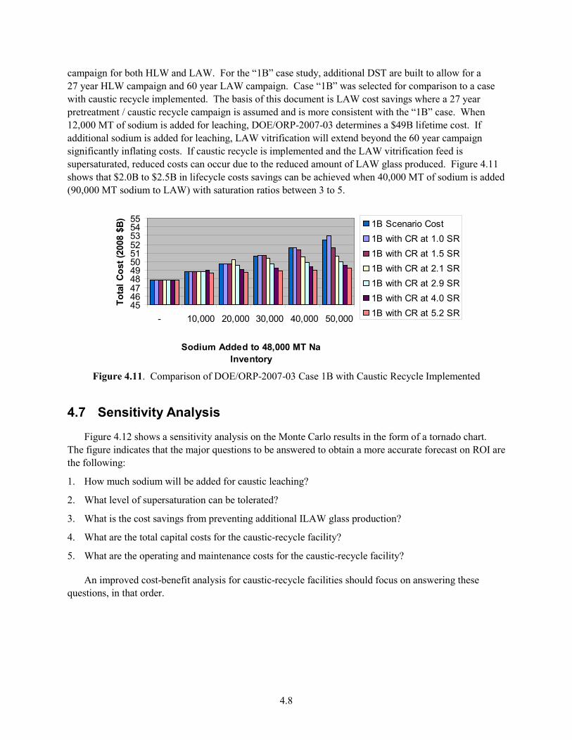
4.11 Comparison of DOE/ORP-2007-03 Case 1B with Caustic Recycle Implemented ..................... 4.8

4.12 Tornado Chart Illustrating the Sensitivity of the Model Parameters on ROI .............................. 4.9

xi

Tables

3.1 Composition of WTP Stream Significant to Caustic Recycle; Adapted From Kirkbride and Coworkers ................................................................................................................................... 3.2

3.2 Composition of WTP Streams Significant to Caustic Recycle With Variable Sodium Addition for Caustic Leaching; Adapted From Kirkbride and Coworkers ................................. 3.4

3.3 Estimation of ILAW Immobilization Costs; adapted from Curtis in 2008 Dollars Assuming 3% Annual Rate of Inflation ....................................................................................................... 3.9

3.4 Monte Carlo Distribution Assumptions for ILAW Cost Savings ............................................... 3.9

3.5 Monte Carlo Distribution Assumptions for Sodium Transport Efficiency ................................. 3.9

3.6 Monte Carlo Distribution Assumptions for Capital Costs of Caustic Recycle Facility .............. 3.11

3.7 Monte Carlo Distribution Assumptions for LAW Vitrification Labor Costs.............................. 3.12

3.8 Monte Carlo Distribution Assumptions for Estimated Labor Costs ........................................... 3.12

3.9 Monte Carlo Distribution Assumptions for Electrochemical Cell Potential ............................... 3.13

3.10 Monte Carlo Distribution Assumptions for Electricity Prices .................................................... 3.13

3.11 Monte Carlo Distribution Assumptions for Membrane Replacement Frequency ....................... 3.14

3.12 Monte Carlo Distribution Assumptions for Membrane Replacement Costs ............................... 3.14

3.13 Monte Carlo Distribution Assumptions for Research and Technology Costs ............................ 3.15

3.14 Basis to Eliminate Total Capital Investment ............................................................................... 3.15

3.15 Basis to Estimate Operating and Maintenance Costs .................................................................. 3.16

3.16 Cost Benefit Terms and Basis for Calculation ............................................................................ 3.17

1.1

1.0 Introduction

Sodium is one of the most common components of the Hanford tank wastes and is a major contributor to the waste-oxide loading in the low-activity waste (LAW) glass. In addition to the large amounts of sodium already in the wastes, the current waste-treatment approach calls for adding additional sodium (primarily as NaOH) while pretreating the tank wastes, which would help control corrosion in the tank farms and also potentially increase the volume of LAW glass. Since the tank wastes already contain significant amounts of sodium, there is a potential benefit for a caustic-recycle process that would separate sodium hydroxide for recycle at the Hanford site. This would reduce the volume of LAW glass and minimize the need to purchase new NaOH.

The current pretreatment flowsheet indicates that approximately 6500 metric tons (MT) of Na will be added to the tank waste, primarily for removing Al from the high-level waste (HLW) sludge (Kirkbride et al. 2007). An assessment (Alexander et al. 2004) of the pretreatment flowsheet, equilibrium chemistry, and laboratory results indicates that the quantity of Na required for sludge leaching will increase by 6000 to 12,000 MT in order to dissolve sufficient Al from the tank-waste sludge material to maintain the number of HLW canisters produced at 9,400 canisters as defined in the Office of River Protection (ORP) System Plan (Certa 2003). This additional Na will significantly increase the volume of LAW glass and extend the processing time of the Waste Treatment and Immobilization Plant (WTP). Future estimates on sodium requirements for caustic leaching are expected to significantly exceed the 12,000-MT value and approach 40,000-MT of total sodium addition for leaching (Gilbert, 2007).

Electrochemical salt-splitting technologies for caustic recycle were investigated in the 1990s for application to the treatment of tank wastes at the Hanford, Savannah River, and Idaho National Engineering Laboratory sites. These investigations, which were primarily funded by the EM-50 Efficient Separations and Processing Program, included testing of commercially available, organic-based, ion exchange membranes (i.e., Nafion) and ceramic-based, sodium-selective membranes (NaSICON) developed by Ceramatec Inc. Both membrane types were tested with simulants at the pilot scale and with actual radioactive-waste samples at the bench scale. The Nafion membranes were found to have a lower current efficiency than the ceramic membranes, and they transported radioactive cesium at a higher rate than the sodium, resulting in a contaminated caustic product.

The likely increase in caustic demand for pretreating the tank wastes has resulted in renewed interest in caustic-recycle methods. Ceramatec Inc. has continued to develop the NaSICON membranes for caustic recycle. As part of this development effort, Ceramatec has engaged staff at Pacific Northwest National Laboratory (PNNL) to assist with applying this technology for caustic recycling at Hanford. This report addresses the economics involved in the deployment of such a facility at Hanford.

2.1

2.0 Scope and Objectives

This report contains a review of potential cost benefits of NaSICON Ceramic membranes for the separation of sodium from Hanford tank waste. The primary application is for caustic recycle to the WTP pretreatment leaching operation. The report includes a description of the waste, identification of the benefits and costs for a caustic recycle facility, and Monte Carlo results obtained from a model of these costs and benefits. The use of existing cost information has been limited to publicly available sources. This study is intended to be an initial evaluation of the economic feasibility of a caustic-recycle facility based on NaSICON technology.

3.1

3.0 Methods

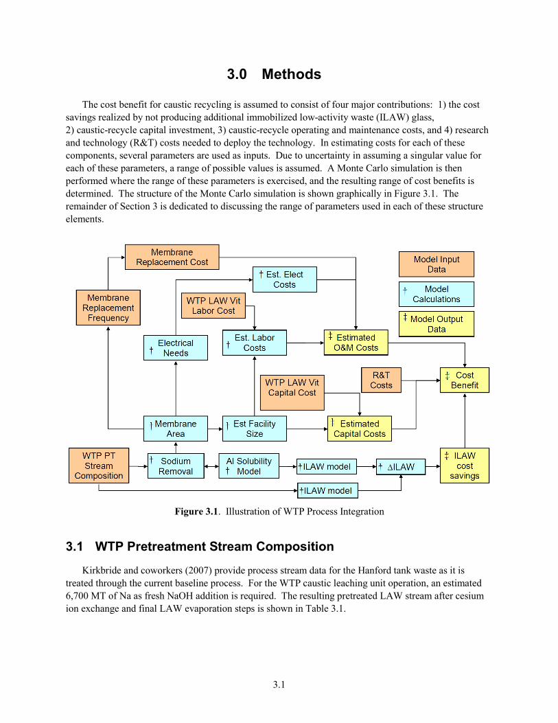
The cost benefit for caustic recycling is assumed to consist of four major contributions: 1) the cost savings realized by not producing additional immobilized low-activity waste (ILAW) glass, 2) caustic-recycle capital investment, 3) caustic-recycle operating and maintenance costs, and 4) research and technology (R&T) costs needed to deploy the technology. In estimating costs for each of these components, several parameters are used as inputs. Due to uncertainty in assuming a singular value for each of these parameters, a range of possible values is assumed. A Monte Carlo simulation is then performed where the range of these parameters is exercised, and the resulting range of cost benefits is determined. The structure of the Monte Carlo simulation is shown graphically in Figure 3.1. The remainder of Section 3 is dedicated to discussing the range of parameters used in each of these structure elements.

Figure 3.1. Illustration of WTP Process Integration

3.1 WTP Pretreatment Stream Composition

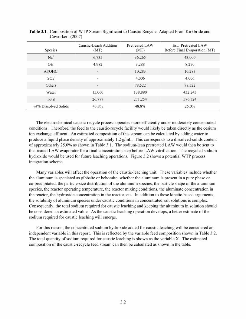
Kirkbride and coworkers (2007) provide process stream data for the Hanford tank waste as it is treated through the current baseline process. For the WTP caustic leaching unit operation, an estimated 6,700 MT of Na as fresh NaOH addition is required. The resulting pretreated LAW stream after cesium ion exchange and final LAW evaporation steps is shown in Table 3.1.

3.2

Table 3.1. Composition of WTP Stream Significant to Caustic Recycle; Adapted From Kirkbride and Coworkers (2007)

Species Caustic-Leach Addition

(MT) Pretreated LAW

(MT) Est. Pretreated LAW

Before Final Evaporation (MT)

Na+ 6,735 36,265 43,000

OH- 4,982 3,288 8,270

Al(OH)4- - 10,283 10,283

SO4- - 4,006 4,006

Others - 78,522 78,522

Water 15,060 138,890 432,243

Total 26,777 271,254 576,324

wt% Dissolved Solids 43.8% 48.8% 25.0%

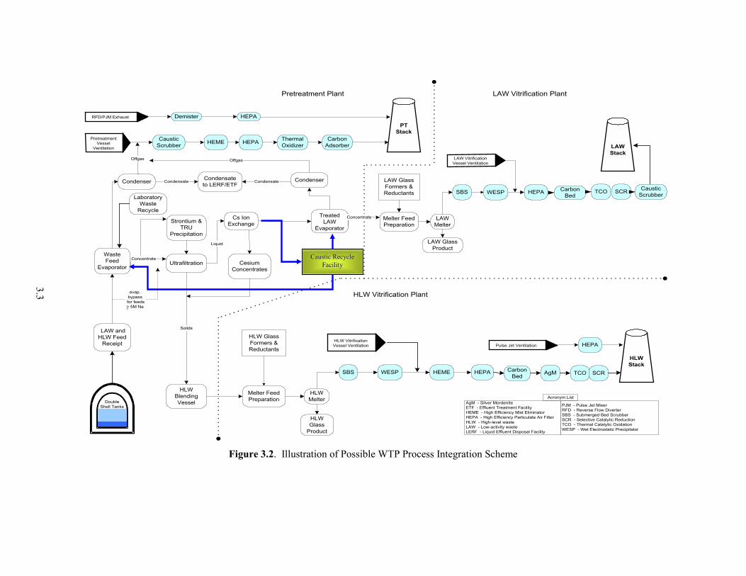
The electrochemical caustic-recycle process operates more efficiently under moderately concentrated conditions. Therefore, the feed to the caustic-recycle facility would likely be taken directly as the cesium ion exchange effluent. An estimated composition of this stream can be calculated by adding water to produce a liquid phase density of approximately 1.2 g/mL. This corresponds to a dissolved-solids content of approximately 25.0% as shown in Table 3.1. The sodium-lean pretreated LAW would then be sent to the treated LAW evaporator for a final concentration step before LAW vitrification. The recycled sodium hydroxide would be used for future leaching operations. Figure 3.2 shows a potential WTP process integration scheme.

Many variables will affect the operation of the caustic-leaching unit. These variables include whether the aluminum is speciated as gibbsite or behomite, whether the aluminum is present in a pure phase or co-precipitated, the particle-size distribution of the aluminum species, the particle shape of the aluminum species, the reactor operating temperature, the reactor mixing conditions, the aluminate concentration in the reactor, the hydroxide concentration in the reactor, etc. In addition to these kinetic-based arguments, the solubility of aluminum species under caustic conditions in concentrated salt solutions is complex. Consequently, the total sodium required for caustic leaching and keeping the aluminum in solution should be considered an estimated value. As the caustic-leaching operation develops, a better estimate of the sodium required for caustic leaching will emerge.

For this reason, the concentrated sodium hydroxide added for caustic leaching will be considered an independent variable in this report. This is reflected by the variable feed composition shown in Table 3.2. The total quantity of sodium required for caustic leaching is shown as the variable X. The estimated composition of the caustic-recycle feed stream can then be calculated as shown in the table.

3.3

HLW GlassFormers &Reductants

Melter FeedPreparation

HLWMelter

SBS WESP HEME HEPA

HLWGlass

Product

LAW GlassProduct

Condensateto LERF/ETF

CesiumConcentrates

AgM

LAW Vitrification PlantPretreatment Plant

HLW Vitrification Plant

LAW andHLW Feed

Receipt

WasteFeed

Evaporator

LAW GlassFormers &Reductants

LAWMelter

SBS WESP

Ultrafiltration

Strontium &TRU

Precipitation

HEPA

Melter FeedPreparation

HLWBlendingVessel

Cs IonExchange

TreatedLAW

Evaporator

Liquid

Condensate

Solids

Concentrate

Condenser

CausticScrubber

HLW VitrificationVessel Ventilation

PJM - Pulse Jet Mixer RFD - Reverse Flow Diverter SBS - Submerged Bed Scrubber SCR - Selective Catalytic Reduction TCO - Thermal Catalytic Oxidation WESP - Wet Electrostatic Precipitator

AgM - Silver Mordenite ETF - Effluent Treatment Facility HEME - High Efficiency Mist Eliminator HEPA - High Efficiency Particulate Air Filter HLW - High-level waste LAW - Low-activity waste LERF - Liquid Effluent Disposal Facility

Offgas

Pulse Jet Ventilation HEPA

TCO SCR

Acronym List

PTStack

HEME HEPA ThermalOxidizer

CarbonAdsorber

PretreatmentVessel

Ventilation LAWStack

HLWStack

RFD/PJM Exhaust Demister HEPA

DoubleShell Tanks

evap.bypass

for feeds> 5M Na-

LAW VitrificationVessel Ventilation

Condenser

Offgas

Condensate

Concentrate

CarbonBed

TCO SCR CausticScrubber

CarbonBedLaboratory

WasteRecycle

Caustic Recycle Caustic Recycle FacilityFacility

Figure 3.2. Illustration of Possible WTP Process Integration Scheme

3.4

Table 3.2. Composition of WTP Streams Significant to Caustic Recycle With Variable Sodium Addition for Caustic Leaching; Adapted From Kirkbride and Coworkers (2007)

Species Caustic-Leach Addition

(MT) Pretreated LAW

(MT) Est. Pretreated LAW Before

Final Evaporation (MT)

Na+ X 36,265 36,265 + X

OH- 0.74 X 3,288 3,288 + 0.74 X

Al(OH)4- - 10,283 10,283

SO4- - 4,006 4,006

Others - 78,522 78,522

Water 2.24 X 138,890 535,982 + 7.46X

Total 3.98 X 271,254 668,346 + 9.2 X

Wt% Dissolved Solids 43.8% 48.8% 25.0%

3.2 Sodium Removal

Sodium is recovered via the electrochemical process with a Ceramatec NaSICON membrane as shown in Figure 3.3. Anode, cathode, and overall reactions from this process are shown in the equations below. In this process, sodium ions are selectively transported across a ceramic membrane driven by an applied electrical potential. Anode: 2H2O → O2 + 4H+ + 4e- (3.2.1)

H+ + OH-→ H2O (3.2.2)

Cathode: 4H2O + 4e- → 2H2 + 4OH- (3.2.3)

Overall: 2H2O → 2H2 + O2 (3.2.4)

Na depleted Waste

e-

Pure 50 % Conc. NaOH

Anode Cathode

Dilute caustic

Na+

H2O

O2

H+

H2O

OH-

e- e-

Sodium

LLW stream

Ceramic Membrane Figure 3.3. Schematic of a Two Compartment Electrochemical Process Using the NaSICON Membrane

For every mole of sodium entering the cathode cell, a mole of water is consumed, and a mole of hydroxide ions and half mole of diatomic hydrogen are produced. For every mole of sodium transported

3.5

from the pretreated LAW across the membrane, the anode reaction results in the consumption of a mole of hydroxide ions and the production of half a mole of water and a quarter mole of diatomic oxygen. Consequently, the pH of the pretreated LAW stream drops significantly as the reaction proceeds.

The drop in pretreated LAW pH can be significant enough to precipitate dissolved species in the LAW. This study limits the amount of sodium transported across the membrane to an amount that will not result in aluminate saturation to a series of assumed temperatures. The solubility model used for this sodium-transport constraint is discussed in Section 3.3.

3.3 Aluminum Solubility Model

One limitation of any caustic-recovery stream will be to avoid fouling the caustic recovery cell from the precipitation of aluminum. Therefore, to understand how much caustic can be removed from a process stream, it is necessary to understand the equilibrium conditions between Al and hydroxide.

Misra (1970) developed an empirical model for the quantity of sodium required to dissolve gibbsite from simulant data:

[ ] [ ]NaOHTNaOH

TOHAl ln71.3370.248671.5])(ln[ 4 ++−=− (3.3.1)

where T = temperature in Kelvin [Al(OH)4

-] = concentration in solution [NaOH] = concentration added.

Figure 3.4 provides a summary for the Al solubility for a 2, 4, 6, 8 and 10 -M hydroxide solution as a function of temperature. Note that this equation was developed for pure sodium hydroxide solutions. Other anions will cause some increase in the solubility of aluminum. However, for the sake of conservatively estimating how much caustic can be recovered, we will use the solubility of aluminum based only on the hydroxide concentration of the process streams.

As seen in Figure 3.4, the solubility of gibbsite increases dramatically as the temperature is increased. Note that the baseline process for dissolving aluminum requires cooling of the solution to 25ºC. Therefore, to verify that the Al remains in solution, it will be necessary to keep the Al:NaOH ratio at approximately 0.1 or less.

0.00.10.20.30.40.50.60.70.80.91.0

25 35 45 55 65 75 85 95

Temperature (C)

Al:N

a (M

/M) 2

46810

[NaOH]

Figure 3.4. Gibbsite Solubility – Molarity of Al in Solution for Given Initial Solution NaOH Molarity

3.6

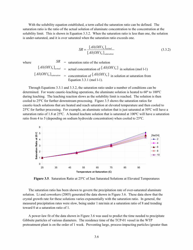
With the solubility equation established, a term called the saturation ratio can be defined. The saturation ratio is the ratio of the actual solution of aluminate concentration to the concentration at the solubility limit. This is shown in Equation 3.3.2. When the saturation ratio is less than one, the solution is under-saturated, and it is over saturated when the saturation ratio exceeds one.

saturation

actual

OHAlOHAl

SR])([])([

4

4−

−

= (3.3.2)

where SR = saturation ratio of the solution

actualOHAl ])([ 4−

= actual concentration of ])([ 4−OHAl in solution (mol l-1)

saturationOHAl ])([ 4−

= concentration of ])([ 4−OHAl in solution at saturation from

Equation 3.3.1 (mol l-1).

Through Equations 3.3.1 and 3.3.2, the saturation ratio under a number of conditions can be determined. For waste caustic-leaching operations, the aluminate solution is heated to 60º to 100ºC during leaching. The leaching reaction slows as the solubility limit is reached. The solution is then cooled to 25ºC for further downstream processing. Figure 3.5 shows the saturation ratios for caustic-leach solutions that are heated and reach saturation at elevated temperature and then cooled to 25ºC for further processing. For example, an aluminate solution that is just saturated at 50ºC will have a saturation ratio of 1.8 at 25ºC. A heated leachate solution that is saturated at 100ºC will have a saturation ratio from 4 to 5 (depending on sodium hydroxide concentration) when cooled to 25ºC.

0

1

2

3

4

5

6

25 35 45 55 65 75 85 95

Temperature at Saturation (C)

Sat

urat

ion

Rat

io a

t 25

C

246810

[NaOH]

Figure 3.5. Saturation Ratio at 25ºC of Just Saturated Solutions at Elevated Temperatures

The saturation ratio has been shown to govern the precipitation rate of over-saturated aluminate solution. Li and coworkers (2005) generated the data shown in Figure 3.6. These data show that the crystal growth rate for these solutions varies exponentially with the saturation ratio. In general, the measured precipitation rates were slow, being under 1 nm/min at a saturation ratio of 8 and trending toward 0 at a saturation ratio of 1.

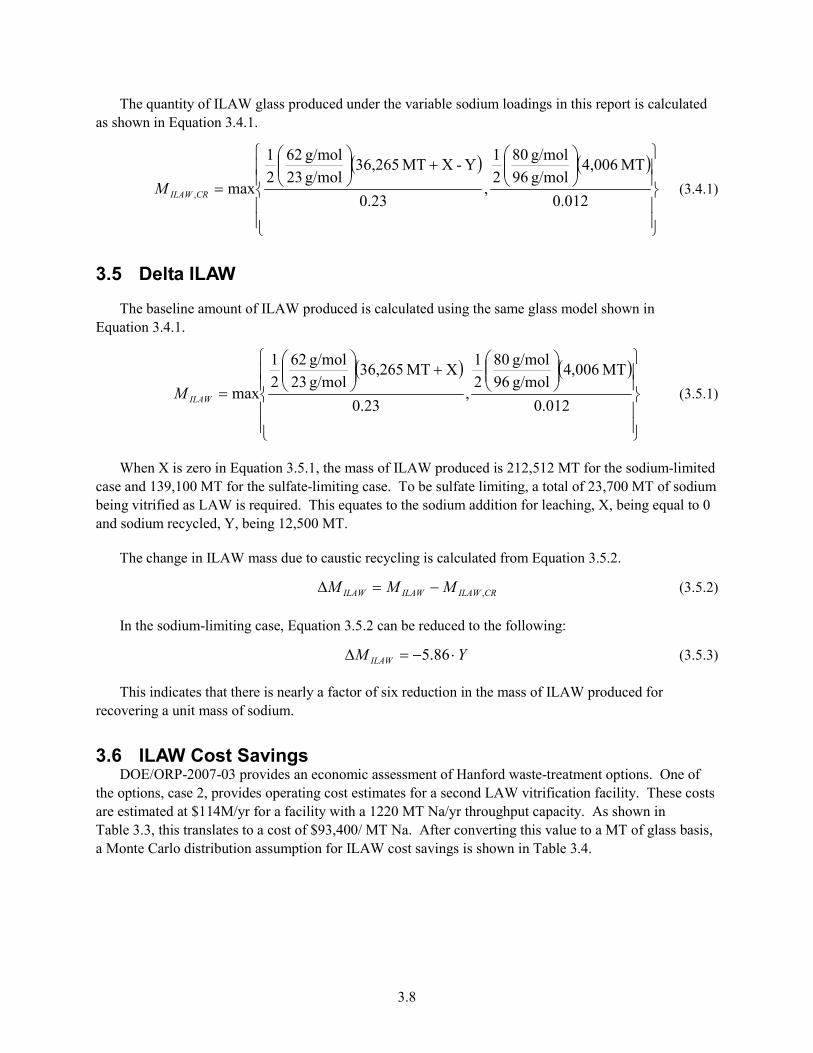
A power-law fit of the data shown in Figure 3.6 was used to predict the time needed to precipitate Gibbsite particles of various diameters. The residence time of the TCP-01 vessel in the WTP pretreatment plant is on the order of 1 week. Preventing large, process-impacting particles (greater than

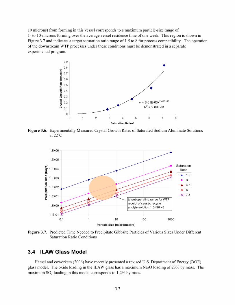
3.7

10 microns) from forming in this vessel corresponds to a maximum particle-size range of 1- to 10-microns forming over the average vessel residence time of one week. This region is shown in Figure 3.7 and indicates a target saturation ratio range of 1.5 to 8 for process compatibility. The operation of the downstream WTP processes under these conditions must be demonstrated in a separate experimental program.

y = 6.01E-03x2.45E+00

R2 = 9.89E-01

0

0.1

0.2

0.3

0.4

0.5

0.6

0.7

0.8

0.9

0 1 2 3 4 5 6 7 8

Saturation Ratio-1

Cry

stal

Gro

wth

Rat

e (n

m/m

in)

Figure 3.6. Experimentally Measured Crystal Growth Rates of Saturated Sodium Aluminate Solutions

at 22ºC

1.E-01

1.E+00

1.E+01

1.E+02

1.E+03

1.E+04

1.E+05

1.E+06

0.1 1 10 100 1000

Particle Size (micrometers)

Prec

ipita

tion

Tim

e (D

ays)

1.5

3

4.5

6

7.5

Saturation Ratio

target operating range for WTP receipt of caustic recycle anolyte solution 1.5<SR <8

Figure 3.7. Predicted Time Needed to Precipitate Gibbsite Particles of Various Sizes Under Different

Saturation Ratio Conditions

3.4 ILAW Glass Model

Hamel and coworkers (2006) have recently presented a revised U.S. Department of Energy (DOE) glass model. The oxide loading in the ILAW glass has a maximum Na2O loading of 23% by mass. The maximum SO3 loading in this model corresponds to 1.2% by mass.

3.8

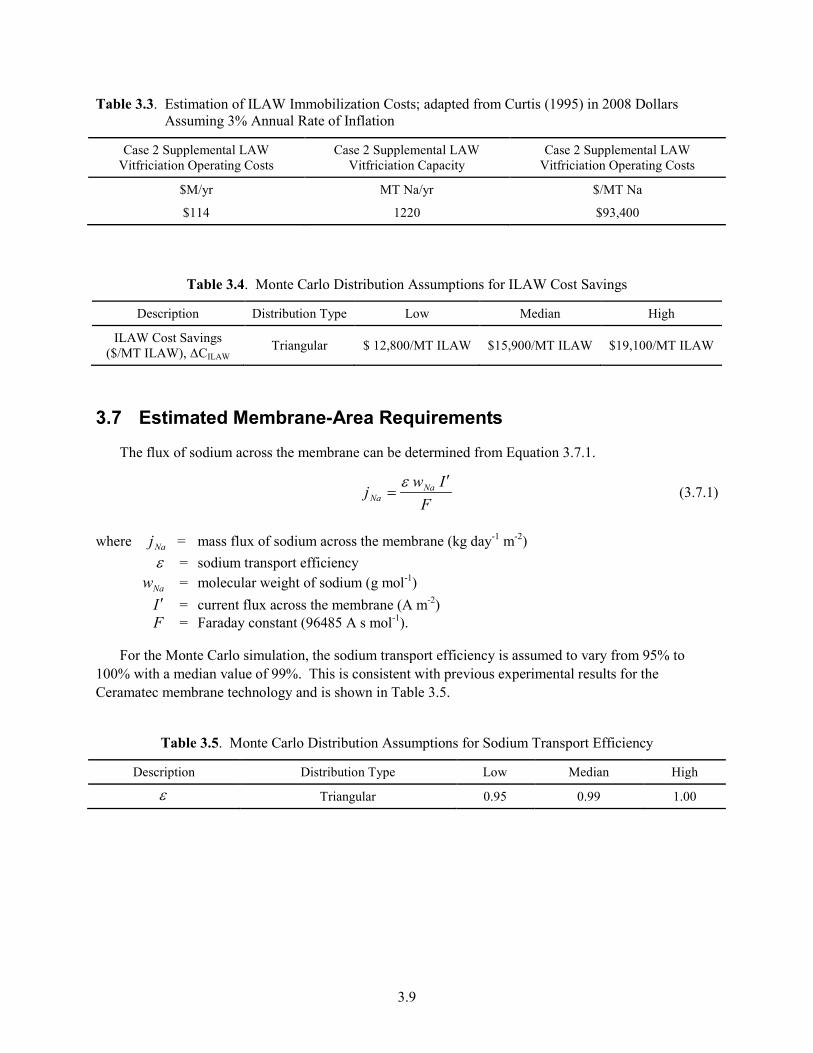
The quantity of ILAW glass produced under the variable sodium loadings in this report is calculated as shown in Equation 3.4.1.

( ) ( )

+

=0.012

MT 4,006g/mol 96g/mol 80

21

,0.23

Y-X MT 36,265g/mol 23g/mol 62

21

max,CRILAWM (3.4.1)

3.5 Delta ILAW

The baseline amount of ILAW produced is calculated using the same glass model shown in Equation 3.4.1.

( ) ( )

+

=0.012

MT 4,006g/mol 96g/mol 80

21

,0.23

X MT 36,265g/mol 23g/mol 62

21

maxILAWM (3.5.1)

When X is zero in Equation 3.5.1, the mass of ILAW produced is 212,512 MT for the sodium-limited case and 139,100 MT for the sulfate-limiting case. To be sulfate limiting, a total of 23,700 MT of sodium being vitrified as LAW is required. This equates to the sodium addition for leaching, X, being equal to 0 and sodium recycled, Y, being 12,500 MT.

The change in ILAW mass due to caustic recycling is calculated from Equation 3.5.2.

CRILAWILAWILAW MMM ,−=∆ (3.5.2)

In the sodium-limiting case, Equation 3.5.2 can be reduced to the following:

YM ILAW ⋅−=∆ 86.5 (3.5.3)

This indicates that there is nearly a factor of six reduction in the mass of ILAW produced for recovering a unit mass of sodium.

3.6 ILAW Cost Savings DOE/ORP-2007-03 provides an economic assessment of Hanford waste-treatment options. One of

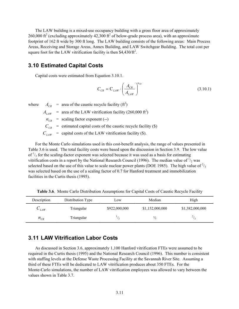
the options, case 2, provides operating cost estimates for a second LAW vitrification facility. These costs are estimated at $114M/yr for a facility with a 1220 MT Na/yr throughput capacity. As shown in Table 3.3, this translates to a cost of $93,400/ MT Na. After converting this value to a MT of glass basis, a Monte Carlo distribution assumption for ILAW cost savings is shown in Table 3.4.

3.9

Table 3.3. Estimation of ILAW Immobilization Costs; adapted from Curtis (1995) in 2008 Dollars Assuming 3% Annual Rate of Inflation

Case 2 Supplemental LAW Vitfriciation Operating Costs

Case 2 Supplemental LAW Vitfriciation Capacity

Case 2 Supplemental LAW Vitfriciation Operating Costs

$M/yr MT Na/yr $/MT Na

$114 1220 $93,400

Table 3.4. Monte Carlo Distribution Assumptions for ILAW Cost Savings

Description Distribution Type Low Median High

ILAW Cost Savings ($/MT ILAW), ΔCILAW Triangular $ 12,800/MT ILAW $15,900/MT ILAW $19,100/MT ILAW

3.7 Estimated Membrane-Area Requirements

The flux of sodium across the membrane can be determined from Equation 3.7.1.

F

Iwj Na

Na

′=ε

(3.7.1)

where Naj = mass flux of sodium across the membrane (kg day-1 m-2) ε = sodium transport efficiency Naw = molecular weight of sodium (g mol-1) I ′ = current flux across the membrane (A m-2) F = Faraday constant (96485 A s mol-1).

For the Monte Carlo simulation, the sodium transport efficiency is assumed to vary from 95% to 100% with a median value of 99%. This is consistent with previous experimental results for the Ceramatec membrane technology and is shown in Table 3.5.

Table 3.5. Monte Carlo Distribution Assumptions for Sodium Transport Efficiency


ε Triangular 0.95 0.99 1.00

3.10

The membrane area needed is then determined by Equation 3.7.2

Na

NaNa j

QRA = (3.7.2)

where NaA = total membrane area required (m2)

NaR = quantity of sodium to be recovered per unit volume of feed (kg L-1)

Q = maximum flow rate to be input to the caustic-recovery facility (L min-1).

3.8 Estimated Facility Size

A preliminary layout for a caustic-recycle facility was created as part of this project. The facility consists of an electrochemical cell area approximately 60 feet by 35 feet. Twenty electrochemical cell modules were contained in this area, producing a ratio of 100 ft2 per module. The remainder of the facility consists of feed and product tanks, piping, and pumps. Since the same volume of feed is expected to be processed through the facility regardless of the amount of caustic recovered, this area was assumed to remain constant regardless of the number of electrochemical modules required. The total facility footprint was approximately 70 feet by 120 feet. Subtracting out the area for the electrochemical modules produces 6,420 ft2.

Each module contains 40 scaffolds, and each scaffold contains 48 disk membranes. Each disk membrane has a surface area of 45.6 cm2. This design results in 8.8 m2 of membrane area per module. The total facility size based on the required membrane area is shown in Equation 3.8.1.

22

2

ft 6420m

modules8.8module

ft100 +

⋅

= NaCR AA (3.8.1)

where CRA = area of the caustic recycle facility (ft2)

NaA = total membrane area required (m2).

3.9 LAW Vitrification Facility Costs

DOE/ORP-2007-03 estimates the cost for the LAW vitrification facility to be $1.152B according to the U.S. Army Corps of Engineers (ACE 2006). These costs include the following:

• Direct costs

– Equipment, installation, instrumentation, piping, electrical, insulation, painting, etc.

– Buildings, process and auxiliary

• Indirect costs

– Engineering and supervision

– Construction expense and contractor fee

– Contingency.

3.11

The LAW building is a mixed-use occupancy building with a gross floor area of approximately 260,000 ft2 (excluding approximately 42,300 ft2 of below-grade process area), with an approximate footprint of 162 ft wide by 300 ft long. The LAW building consists of the following areas: Main Process Areas, Receiving and Storage Areas, Annex Building, and LAW Switchgear Building. The total cost per square foot for the LAW vitrification facility is then $4,430/ft2.

3.10 Estimated Capital Costs

Capital costs were estimated from Equation 3.10.1.

CRn

LAW

CRLAWCR A

AC

⋅= C (3.10.1)


LAWA = area of the LAW vitrification facility (260,000 ft2) CRn = scaling factor exponent (--) CRC = estimated capital costs of the caustic recycle facility ($) LAWC = capital costs of the LAW vitrification facility ($).

For the Monte Carlo simulations used in this cost-benefit analysis, the range of values presented in Table 3.6 is used. The total facility costs were based upon the discussion in Section 3.9. The low value of 1/3 for the scaling-factor exponent was selected because it was used as a basis for estimating vitrification costs in a report by the National Research Council (1996). The median value of 1/2 was selected based on the use of this value to scale nuclear power plants (DOE 1985). The high value of 2/3 was selected based on the use of a scaling factor of 0.7 for Hanford treatment and immobilization facilities in the Curtis thesis (1995).

Table 3.6. Monte Carlo Distribution Assumptions for Capital Costs of Caustic Recycle Facility


LAWC Triangular $922,000,000 $1,152,000,000 $1,382,000,000

CRn Triangular 1/3 ½ 2/3

3.11 LAW Vitrification Labor Costs

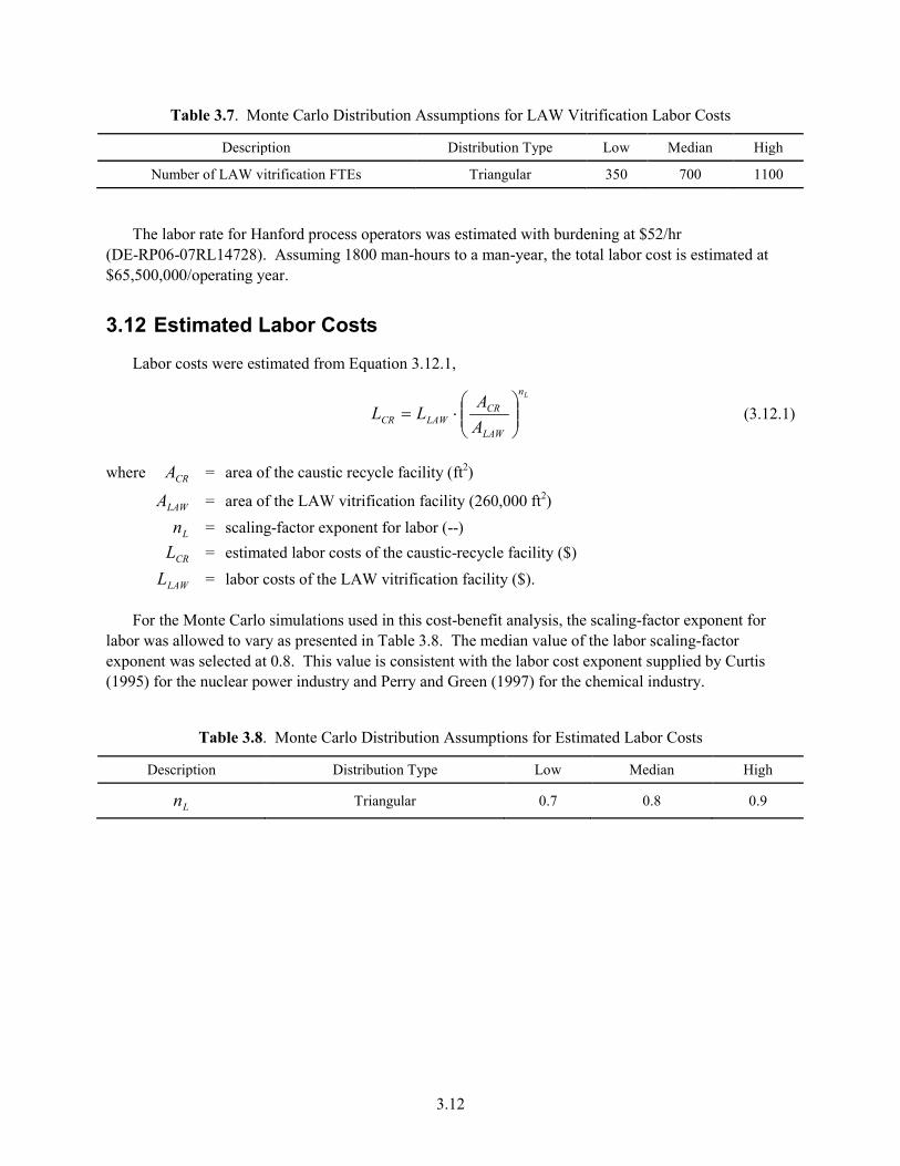
As discussed in Section 3.6, approximately 1,100 Hanford vitrification FTEs were assumed to be required in the Curtis thesis (1995) and the National Research Council (1996). This number is consistent with staffing levels at the Defense Waste Processing Facility at the Savannah River Site. Assuming a third of these FTEs will be dedicated to LAW vitrification produces about 350 FTEs. For the Monte-Carlo simulations, the number of LAW vitrification employees was allowed to vary between the values shown in Table 3.7.

3.12

Table 3.7. Monte Carlo Distribution Assumptions for LAW Vitrification Labor Costs


Number of LAW vitrification FTEs Triangular 350 700 1100

The labor rate for Hanford process operators was estimated with burdening at $52/hr (DE-RP06-07RL14728). Assuming 1800 man-hours to a man-year, the total labor cost is estimated at $65,500,000/operating year.

3.12 Estimated Labor Costs

Labor costs were estimated from Equation 3.12.1,

Ln

LAW

CRLAWCR A

ALL

⋅= (3.12.1)


LAWA = area of the LAW vitrification facility (260,000 ft2) Ln = scaling-factor exponent for labor (--) CRL = estimated labor costs of the caustic-recycle facility ($) LAWL = labor costs of the LAW vitrification facility ($).

For the Monte Carlo simulations used in this cost-benefit analysis, the scaling-factor exponent for labor was allowed to vary as presented in Table 3.8. The median value of the labor scaling-factor exponent was selected at 0.8. This value is consistent with the labor cost exponent supplied by Curtis (1995) for the nuclear power industry and Perry and Green (1997) for the chemical industry.

Table 3.8. Monte Carlo Distribution Assumptions for Estimated Labor Costs


Ln Triangular 0.7 0.8 0.9

3.13

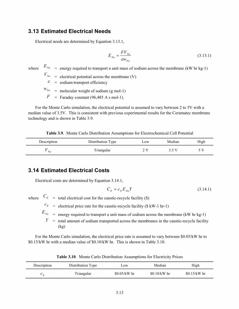
3.13 Estimated Electrical Needs

Electrical needs are determined by Equation 3.13.1,

Na

NaNa w

FVE

ε= (3.13.1)

where NaE = energy required to transport a unit mass of sodium across the membrane (kW hr kg-1)

NaV = electrical potential across the membrane (V) ε = sodium-transport efficiency

Naw = molecular weight of sodium (g mol-1) F = Faraday constant (96,485 A s mol-1).

For the Monte Carlo simulation, the electrical potential is assumed to vary between 2 to 5V with a median value of 3.5V. This is consistent with previous experimental results for the Ceramatec membrane technology and is shown in Table 3.9.

Table 3.9. Monte Carlo Distribution Assumptions for Electrochemical Cell Potential


NaV Triangular 2 V 3.5 V 5 V

3.14 Estimated Electrical Costs

Electrical costs are determined by Equation 3.14.1,

YEcC NaEE = (3.14.1)

where EC = total electrical cost for the caustic-recycle facility ($)

Ec = electrical price rate for the caustic-recycle facility ($ kW-1 hr-1)

NaE = energy required to transport a unit mass of sodium across the membrane (kW hr kg-1) Y = total amount of sodium transported across the membranes in the caustic-recycle facility

(kg)

For the Monte Carlo simulation, the electrical price rate is assumed to vary between $0.05/kW hr to $0.15/kW hr with a median value of $0.10/kW hr. This is shown in Table 3.10.

Table 3.10. Monte Carlo Distribution Assumptions for Electricity Prices


Ec Triangular $0.05/kW hr $0.10/kW hr $0.15/kW hr

3.14

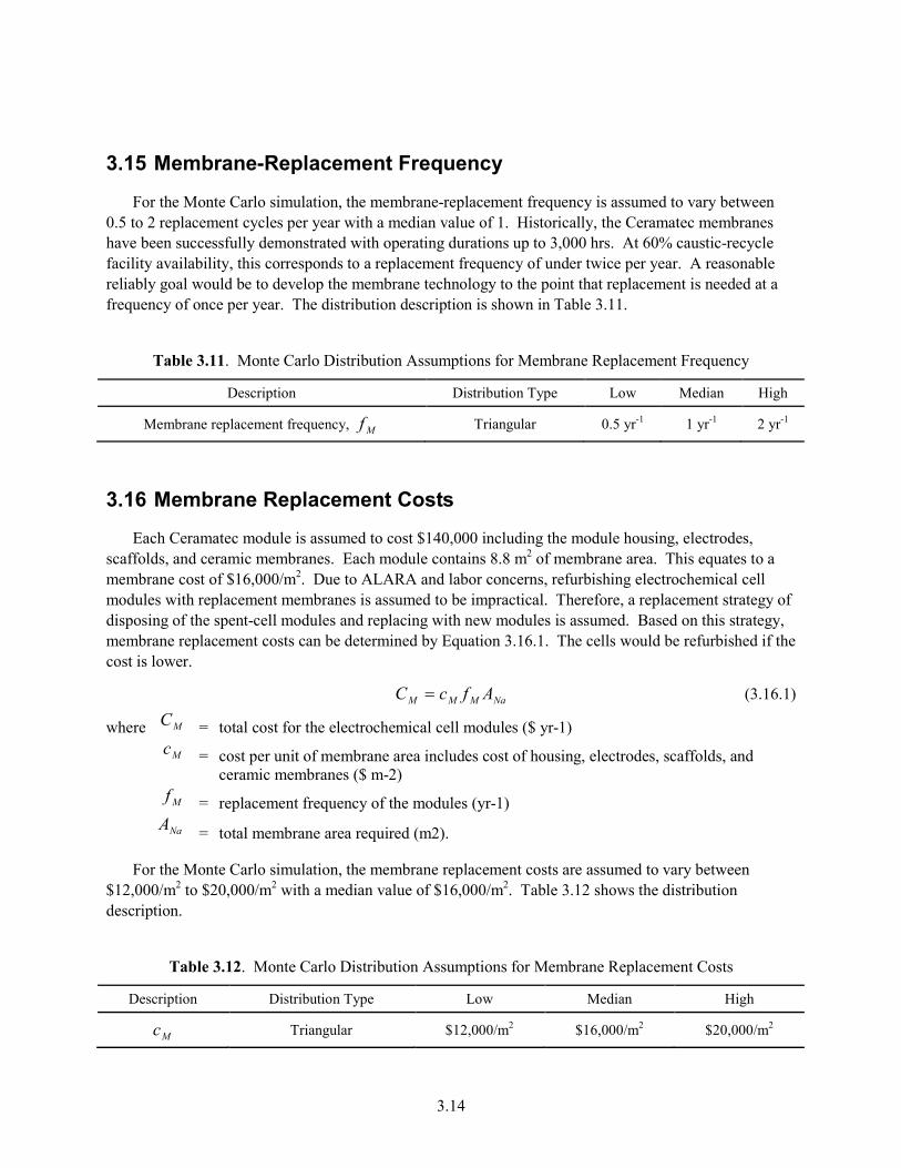
3.15 Membrane-Replacement Frequency

For the Monte Carlo simulation, the membrane-replacement frequency is assumed to vary between 0.5 to 2 replacement cycles per year with a median value of 1. Historically, the Ceramatec membranes have been successfully demonstrated with operating durations up to 3,000 hrs. At 60% caustic-recycle facility availability, this corresponds to a replacement frequency of under twice per year. A reasonable reliably goal would be to develop the membrane technology to the point that replacement is needed at a frequency of once per year. The distribution description is shown in Table 3.11.

Table 3.11. Monte Carlo Distribution Assumptions for Membrane Replacement Frequency


Membrane replacement frequency, Mf Triangular 0.5 yr-1 1 yr-1 2 yr-1

3.16 Membrane Replacement Costs

Each Ceramatec module is assumed to cost $140,000 including the module housing, electrodes, scaffolds, and ceramic membranes. Each module contains 8.8 m2 of membrane area. This equates to a membrane cost of $16,000/m2. Due to ALARA and labor concerns, refurbishing electrochemical cell modules with replacement membranes is assumed to be impractical. Therefore, a replacement strategy of disposing of the spent-cell modules and replacing with new modules is assumed. Based on this strategy, membrane replacement costs can be determined by Equation 3.16.1. The cells would be refurbished if the cost is lower.

NaMMM AfcC = (3.16.1)

where MC = total cost for the electrochemical cell modules ($ yr-1)

Mc = cost per unit of membrane area includes cost of housing, electrodes, scaffolds, and ceramic membranes ($ m-2)

Mf = replacement frequency of the modules (yr-1)

NaA = total membrane area required (m2).

For the Monte Carlo simulation, the membrane replacement costs are assumed to vary between $12,000/m2 to $20,000/m2 with a median value of $16,000/m2. Table 3.12 shows the distribution description.

Table 3.12. Monte Carlo Distribution Assumptions for Membrane Replacement Costs


Mc Triangular $12,000/m2 $16,000/m2 $20,000/m2

3.15

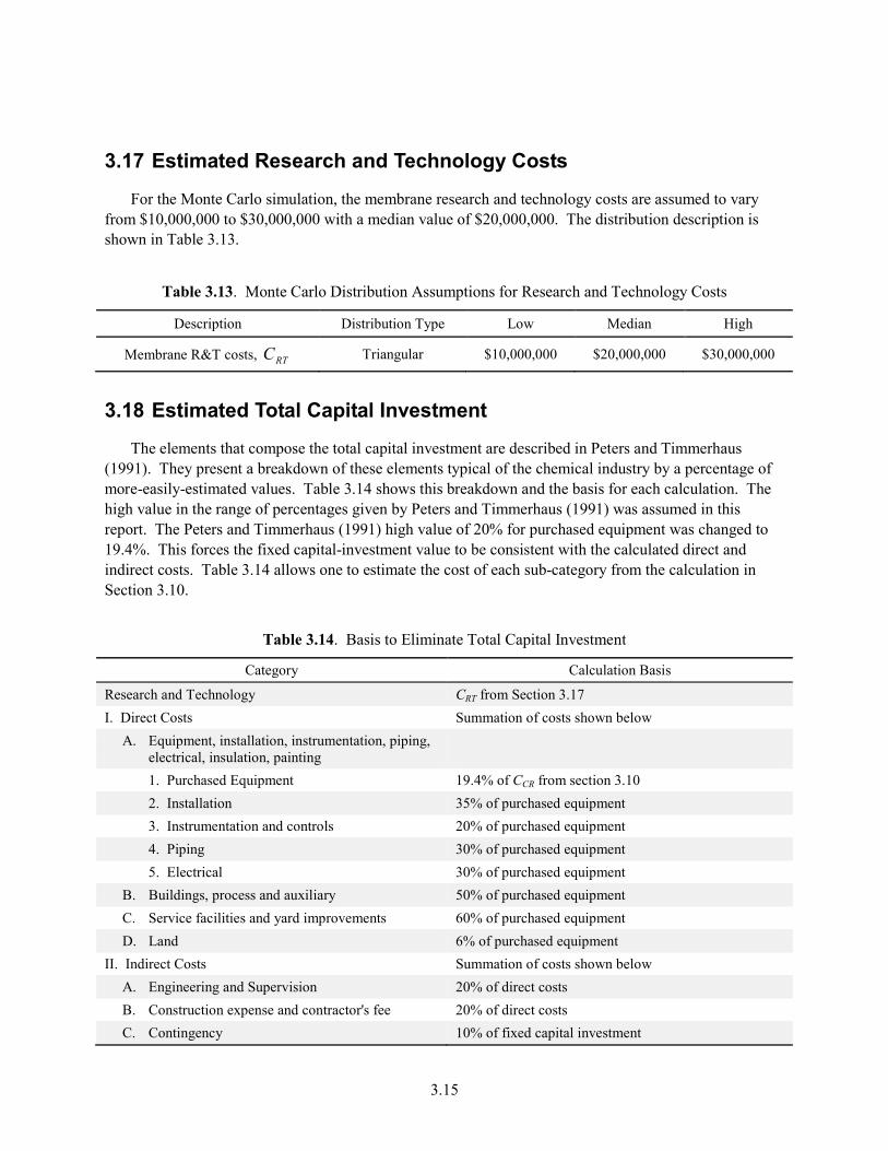
3.17 Estimated Research and Technology Costs

For the Monte Carlo simulation, the membrane research and technology costs are assumed to vary from $10,000,000 to $30,000,000 with a median value of $20,000,000. The distribution description is shown in Table 3.13.

Table 3.13. Monte Carlo Distribution Assumptions for Research and Technology Costs


Membrane R&T costs, RTC Triangular $10,000,000 $20,000,000 $30,000,000

3.18 Estimated Total Capital Investment

The elements that compose the total capital investment are described in Peters and Timmerhaus (1991). They present a breakdown of these elements typical of the chemical industry by a percentage of more-easily-estimated values. Table 3.14 shows this breakdown and the basis for each calculation. The high value in the range of percentages given by Peters and Timmerhaus (1991) was assumed in this report. The Peters and Timmerhaus (1991) high value of 20% for purchased equipment was changed to 19.4%. This forces the fixed capital-investment value to be consistent with the calculated direct and indirect costs. Table 3.14 allows one to estimate the cost of each sub-category from the calculation in Section 3.10.

Table 3.14. Basis to Eliminate Total Capital Investment

Category Calculation Basis

Research and Technology CRT from Section 3.17 I. Direct Costs Summation of costs shown below

A. Equipment, installation, instrumentation, piping, electrical, insulation, painting 1. Purchased Equipment 19.4% of CCR from section 3.10 2. Installation 35% of purchased equipment 3. Instrumentation and controls 20% of purchased equipment 4. Piping 30% of purchased equipment 5. Electrical 30% of purchased equipment

B. Buildings, process and auxiliary 50% of purchased equipment C. Service facilities and yard improvements 60% of purchased equipment D. Land 6% of purchased equipment

II. Indirect Costs Summation of costs shown below A. Engineering and Supervision 20% of direct costs B. Construction expense and contractor's fee 20% of direct costs C. Contingency 10% of fixed capital investment

3.16

Table 3.14. (contd)


III. Fixed Capital Investment CCR from section 3.10 + R&T costs should equal R&T + Direct Costs + Indirect Costs

IV. Working Capital 10% of total capital investment V. Total Capital Investment Fixed Capital Investment + Working Capital

3.19 Estimated Operating and Maintenance Costs

In addition to the estimate for total capital investment, Peters and Timmerhaus (1991) present a similar breakdown for the elements of operating and maintenance costs. Table 3.15 shows this breakdown and the basis for each calculation.

Table 3.15. Basis to Estimate Operating and Maintenance Costs


I. Manufacturing Costs Summation of costs shown below A. Direct Production Costs

1. Raw Materials n/a 2. Operating Labor LCR from Section 3.12 3. Direct supervisory and clerical labor 15% of operating labor 4. Utilities CE from Section 3.14 5. Maintenance 10% of fixed capital investment 6. Operating Supplies 15% of maintenance 7. Laboratory Charges 15% of operating labor 8. Patents and Royalties n/a

B. Fixed Charges Summation of costs shown below 1. Depreciation 10% of equipment 2. Local Taxes n/a 3. Insurance 1% of fixed capital investment 4. Rent 10% of value of the rental property

C. Plant-overhead costs 60% of operating, supervisory, and maintenance II. General Expenses Summation of costs shown below

A. Administrative Costs 15% of operating, supervisory, and maintenance B. Distribution and selling costs n/a C. Research and development costs n/a D. Financing n/a

III. Total Production Cost Manufacturing Costs + General Expenses IV. Gross-earning cost Gross annual sales – Total Production Costs V. Gross annual sales Total LAW Cost Savings, ΔCILAW ΔMILAW

3.17

3.20 Estimated Cost Benefit

From the data calculated from Table 3.14 and Table 3.15, several cost-benefit values can be calculated. These values are shown in Table 3.16 and include specific sales and production costs, turn-over ratio, and total return on investment (ROI). ROI was the primary calculation objective in this report.

Table 3.16. Cost Benefit Terms and Basis for Calculation


Specific Sale Cost/kg Gross annual sales/Sodium Recycled ΔCILAW ΔMILAW /Y Specific Production Cost/kg Total Production Costs/Sodium Recycled Turn-over ratio Gross annual sales/Total Capital Investment Return on Investment Gross earning cost/Total Capital Investment

4.1

4.0 Results

The results discussed in this section include the ROI, the cost savings, the capital costs, the operations and maintenance (O&M) costs, and the sale and production costs. There is also a sensitivity analysis on the Monte Carlo results. All of the results in this section are based on constant value of money in 2008 dollars. A discounted cash flow analysis could be applied to this model and would lead to significantly lower return on investment and cost benefit values. This is due to the cost savings from this project occurring decades in the future while the start-up costs for building and deploying the technology occur decades sooner.

4.1 Return on Investment

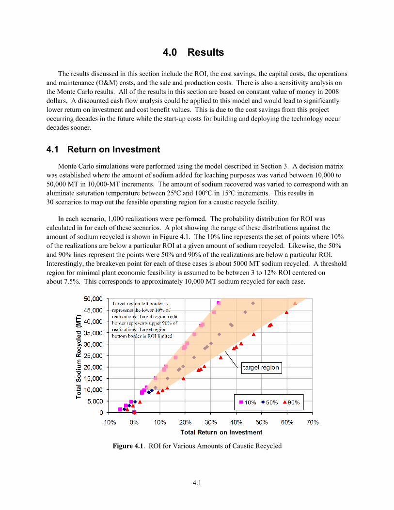
Monte Carlo simulations were performed using the model described in Section 3. A decision matrix was established where the amount of sodium added for leaching purposes was varied between 10,000 to 50,000 MT in 10,000-MT increments. The amount of sodium recovered was varied to correspond with an aluminate saturation temperature between 25ºC and 100ºC in 15ºC increments. This results in 30 scenarios to map out the feasible operating region for a caustic recycle facility.

In each scenario, 1,000 realizations were performed. The probability distribution for ROI was calculated in for each of these scenarios. A plot showing the range of these distributions against the amount of sodium recycled is shown in Figure 4.1. The 10% line represents the set of points where 10% of the realizations are below a particular ROI at a given amount of sodium recycled. Likewise, the 50% and 90% lines represent the points were 50% and 90% of the realizations are below a particular ROI. Interestingly, the breakeven point for each of these cases is about 5000 MT sodium recycled. A threshold region for minimal plant economic feasibility is assumed to be between 3 to 12% ROI centered on about 7.5%. This corresponds to approximately 10,000 MT sodium recycled for each case.

Figure 4.1. ROI for Various Amounts of Caustic Recycled

4.2

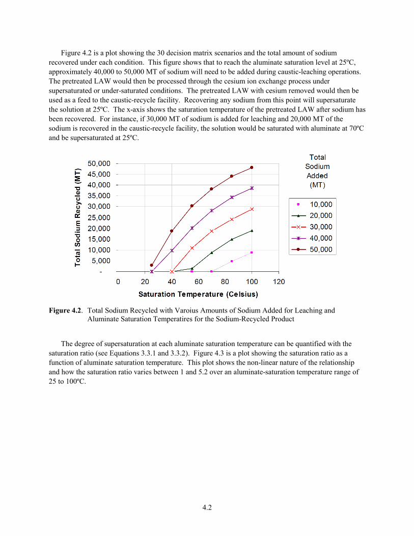
Figure 4.2 is a plot showing the 30 decision matrix scenarios and the total amount of sodium recovered under each condition. This figure shows that to reach the aluminate saturation level at 25ºC, approximately 40,000 to 50,000 MT of sodium will need to be added during caustic-leaching operations. The pretreated LAW would then be processed through the cesium ion exchange process under supersaturated or under-saturated conditions. The pretreated LAW with cesium removed would then be used as a feed to the caustic-recycle facility. Recovering any sodium from this point will supersaturate the solution at 25ºC. The x-axis shows the saturation temperature of the pretreated LAW after sodium has been recovered. For instance, if 30,000 MT of sodium is added for leaching and 20,000 MT of the sodium is recovered in the caustic-recycle facility, the solution would be saturated with aluminate at 70ºC and be supersaturated at 25ºC.

Figure 4.2. Total Sodium Recycled with Varoius Amounts of Sodium Added for Leaching and

Aluminate Saturation Temperatires for the Sodium-Recycled Product

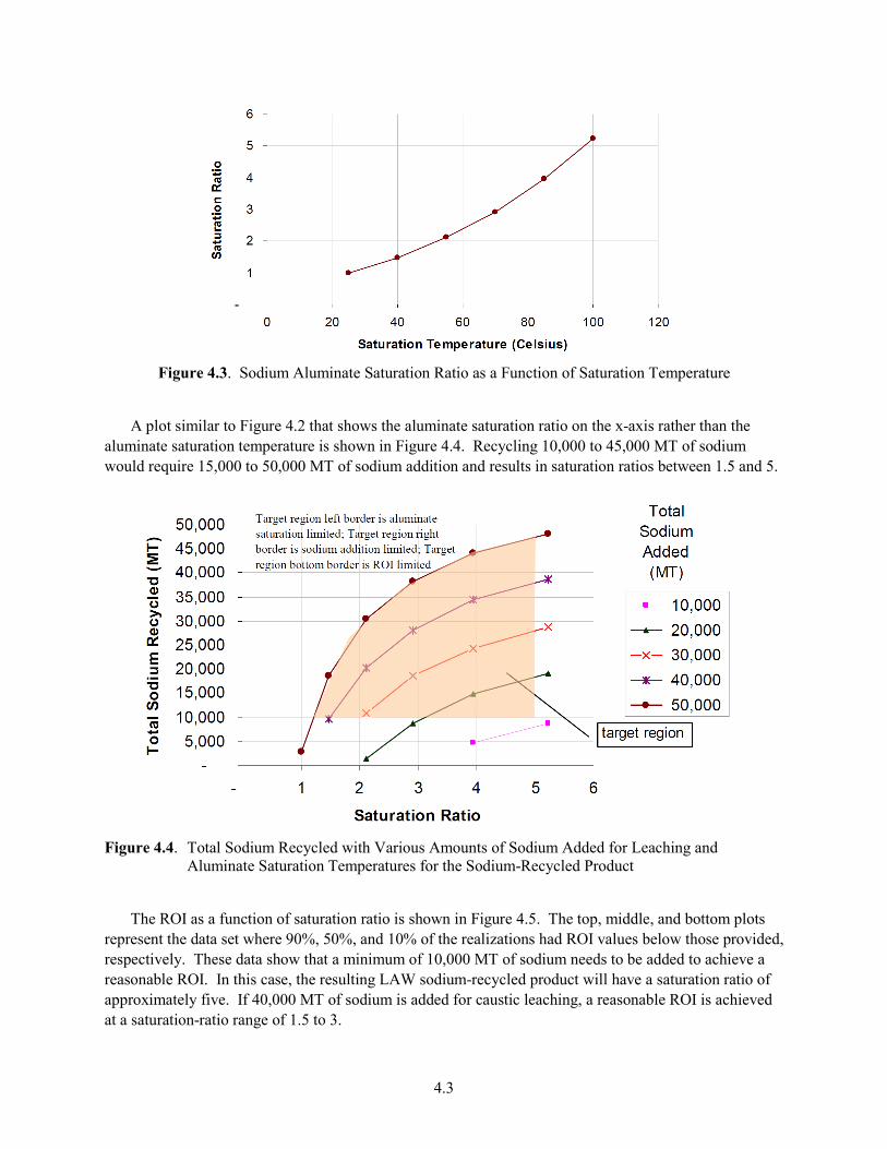
The degree of supersaturation at each aluminate saturation temperature can be quantified with the saturation ratio (see Equations 3.3.1 and 3.3.2). Figure 4.3 is a plot showing the saturation ratio as a function of aluminate saturation temperature. This plot shows the non-linear nature of the relationship and how the saturation ratio varies between 1 and 5.2 over an aluminate-saturation temperature range of 25 to 100ºC.

4.3

Figure 4.3. Sodium Aluminate Saturation Ratio as a Function of Saturation Temperature

A plot similar to Figure 4.2 that shows the aluminate saturation ratio on the x-axis rather than the aluminate saturation temperature is shown in Figure 4.4. Recycling 10,000 to 45,000 MT of sodium would require 15,000 to 50,000 MT of sodium addition and results in saturation ratios between 1.5 and 5.

Figure 4.4. Total Sodium Recycled with Various Amounts of Sodium Added for Leaching and

Aluminate Saturation Temperatures for the Sodium-Recycled Product

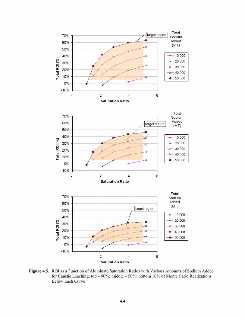
The ROI as a function of saturation ratio is shown in Figure 4.5. The top, middle, and bottom plots represent the data set where 90%, 50%, and 10% of the realizations had ROI values below those provided, respectively. These data show that a minimum of 10,000 MT of sodium needs to be added to achieve a reasonable ROI. In this case, the resulting LAW sodium-recycled product will have a saturation ratio of approximately five. If 40,000 MT of sodium is added for caustic leaching, a reasonable ROI is achieved at a saturation-ratio range of 1.5 to 3.

4.4

Figure 4.5. ROI as a Function of Aluminate Saturation Ratios with Various Amounts of Sodium Added

for Caustic Leaching; top – 90%; middle – 50%; bottom 10% of Monte Carlo Realizations Below Each Curve

4.5

4.2 Cost Savings

The range of specific cost-savings values in this assessment was described in Section 3.6. Figure 4.6 shows the Monte Carlo output for net cost savings as a function of total sodium recycled. If 10,000 MT of sodium is recycled, a cost savings in ILAW glass of $0.7B to $1B would be realized. If 30,000 MT of sodium is recycled, $2.5B to $3.1B would likely be realized.

-

5,000

10,000

15,000

20,000

25,000

30,000

35,000

40,000

45,000

50,000

0 1 2 3 4 5 6

ILAW Cost Savings ($B)

Tota

l Sod

ium

Rec

ycle

d (M

T)

10% 50% 90%

Figure 4.6. ILAW Net Cost Savings as a Function of Total Sodium Recycled

4.3 Capital Costs

The range of total parameters in capital investment calculations in this assessment was described in Section 3.10. Figure 4.7 shows the Monte Carlo output for total capital costs as a function of total sodium recycled. If 10,000 MT of sodium is recycled, a total capital cost for the caustic-recycle facility is estimated to be in the range of $175M to $325M. If 30,000 MT of sodium is recycled, $200M to $350M would likely be realized.

4.4 O&M Costs

The components of the total-production-cost calculation were described in Section 3.19. Figure 4.8 shows the Monte Carlo output for total production costs as a function of total sodium recycled. If 10,000 MT of sodium is recycled, a total production cost for the caustic-recycle facility is estimated to be in the range of $13M/yr to $21M/yr. If 30,000 MT of sodium is recycled, $21M/yr to $30M/yr would likely be realized.

4.6

0

5,000

10,000

15,000

20,000

25,000

30,000

35,000

40,000

45,000

50,000

100 150 200 250 300 350 400

Total Capital Investment ($)

Tota

l Sod

ium

Rec

ycle

d (M

T)

10% 50% 90%

Figure 4.7. Total Capital Investment as a Function of Total Sodium Recycled

0

5,000

10,000

15,000

20,000

25,000

30,000

35,000

40,000

45,000

50,000

10 15 20 25 30 35 40

Total Production Costs ($M/yr)

Tota

l Sod

ium

Rec

ycle

d (M

T)

10% 50% 90%

Figure 4.8. Total Production Costs as a Function of Total Sodium Recycled

4.5 Specific Sale and Production Costs

The components of the specific calculations for sale and production costs were described in Section 3.20. Figure 4.9 shows the Monte Carlo output for specific production costs as a function of total sodium recycled. If 10,000 MT of sodium is recycled, a specific production cost is estimated to be in the range of $25/kg to $45/kg. If 30,000 MT of sodium is recycled, $15/kg to $22/kg would likely be realized.

The Monte Carlo output for specific sales as a function of total sodium recycled is shown in Figure 4.10. In this model, the specific sales cost is invariant with the amount of sodium recycled. A specific sales cost is estimated to be in the range of $84/kg to $104/kg. The specific sales cost is a factor of 3.8 to 6.9 greater than the expected specific production cost range.

4.7

05,000

10,000

15,00020,00025,00030,00035,000

40,00045,00050,000

$10 $20 $30 $40 $50 $60 $70 $80 $90 $100 $110 $120

Specific Production Costs ($/kg Na Recycled)

Tota

l Sod

ium

Rec

ycle

d (M

T)10% 50% 90%

Figure 4.9. Specific Production Costs as a Function of Total Sodium Recycled

0

5,000

10,000

15,000

20,000

25,000

30,000

35,000

40,000

45,000

50,000

$10 $20 $30 $40 $50 $60 $70 $80 $90 $100 $110

Specific Sales Costs ($/kg Na Recycled)

Tota

l Sod

ium

Rec

ycle

d (M

T)

10% 50% 90%

Figure 4.10. Specific Sales Costs as a Function of Total Sodium Recycled

4.6 Impact on Hanford Waste Processing

DOE/ORP-2007-03 states that 60,000 MT of sodium is processed as LAW in the baseline scenarios of that document. This corresponds to 12,000 MT of sodium being added to the 48,000 MT sodium inventory in the waste tanks. The “1A” case was limited by LAW throughput and yielded a 60 year

4.8

campaign for both HLW and LAW. For the “1B” case study, additional DST are built to allow for a 27 year HLW campaign and 60 year LAW campaign. Case “1B” was selected for comparison to a case with caustic recycle implemented. The basis of this document is LAW cost savings where a 27 year pretreatment / caustic recycle campaign is assumed and is more consistent with the “1B” case. When 12,000 MT of sodium is added for leaching, DOE/ORP-2007-03 determines a $49B lifetime cost. If additional sodium is added for leaching, LAW vitrification will extend beyond the 60 year campaign significantly inflating costs. If caustic recycle is implemented and the LAW vitrification feed is supersaturated, reduced costs can occur due to the reduced amount of LAW glass produced. Figure 4.11 shows that $2.0B to $2.5B in lifecycle costs savings can be achieved when 40,000 MT of sodium is added (90,000 MT sodium to LAW) with saturation ratios between 3 to 5.

4546474849505152535455

- 10,000 20,000 30,000 40,000 50,000

Sodium Added to 48,000 MT Na Inventory

Tota

l Cos

t (20

08 $

B) 1B Scenario Cost1B with CR at 1.0 SR1B with CR at 1.5 SR1B with CR at 2.1 SR1B with CR at 2.9 SR1B with CR at 4.0 SR1B with CR at 5.2 SR

Figure 4.11. Comparison of DOE/ORP-2007-03 Case 1B with Caustic Recycle Implemented

4.7 Sensitivity Analysis

Figure 4.12 shows a sensitivity analysis on the Monte Carlo results in the form of a tornado chart. The figure indicates that the major questions to be answered to obtain a more accurate forecast on ROI are the following:

1. How much sodium will be added for caustic leaching?

2. What level of supersaturation can be tolerated?

3. What is the cost savings from preventing additional ILAW glass production?

4. What are the total capital costs for the caustic-recycle facility?

5. What are the operating and maintenance costs for the caustic-recycle facility?

An improved cost-benefit analysis for caustic-recycle facilities should focus on answering these questions, in that order.

4.9

10,000

40

0.41

$14,183

$1.02

926.96

0.74

50,000

100

0.59

$17,708

$1.28

512.20

0.86

-20% 0% 20% 40% 60%

Total Sodium Added (MT)

Treated LAW Saturation Temperature (º C)

Fixed Capital Size Exponent (-)

ILAW Savings ($/MT ILAW)

LAW Fixed Capital Investment ($B)

LAW FTEs (-)

Operating Labor Size Exponent (-)

Total Return on Investment

Figure 4.12. Tornado Chart Illustrating the Sensitivity of the Model Parameters on ROI

5.1

5.0 Conclusions

The major conclusions from the Monte Carlo model results discussed in this report are summarized below:

• A feasible region for minimal plant economics (e.g; 10% total return on investment) corresponds to approximately 10,000 MT sodium recycled. Total return on investments in the range of 30%-60% can be achieved when 50,000 MT of sodium are recycled.

• Literature data for the growth rate of Gibbsite particles indicates that particles forming in the 1- to 10-micron range over the average vessel residence time of 1 week corresponds to a saturation ratio less than eight. The operation of the downstream WTP processes under these conditions and with particles of this size must be demonstrated in a separate experimental program.

• Recycling 10,000 MT of sodium results in a cost savings in ILAW glass of $0.7B to $1.0B. If 30,000 MT of sodium is recycled, $2.5B to $3.1B would likely be realized.

• Recycling 10,000 MT of sodium results in an estimated range of total capital cost for the caustic-recycle facility to be $175M to $325M. If 30,000 MT of sodium is recycled, $200M to $350M would likely be realized.

• Recycling 10,000 MT of sodium results in a total production cost for the caustic-recycle facility to be in the range of $13M/yr to $21M/yr. If 30,000 MT of sodium is recycled, $21M/yr to $30M/yr would likely be realized.

• If 10,000 MT of sodium is recycled, a specific production cost is estimated to be in the range of $25/kg to $45/kg. If 30,000 MT of sodium is recycled, $15/kg to $22/kg would likely be realized.

• The specific sales cost is invariant with the amount of sodium recycled. A specific sales cost is estimated to be in the range of $84/kg to $104/kg. The specific sales cost is a factor of 3.8 to 6.9 greater than the expected specific production cost range.

• An improved cost benefit analysis for caustic recycle facilities should focus on improving the basis for the following questions (listed in priority): How much sodium will be added for caustic leaching?

– What level of supersaturation can be tolerated?

– What is the cost savings from preventing additional ILAW glass production?

– What are the total capital costs for the caustic-recycle facility?

– What are the operating and maintenance costs for the caustic-recycle facility?

6.1

6.0 References

ACE (see U.S. Army Corps of Engineers)

Alexander, DL, et al., Design Oversight Report, HLW Feed Preparation System; Ultra-filtration Process System, D-03-DESIGN-005, April 2004.

Certa PJ. 2003. River Protection Project System Plan. ORP-11242 Revision 2, CH2M HILL Hanford Group Inc., Richland, Washington.

Curtis JH. 1995. Economic Considerations for Hanford Tank Waste Disposition. Masters Thesis, Department of Nuclear Engineering, Massachusetts Institute of Technology.

DeMuth S, and DE Kurath. 1998. Cost Benefit of Caustic Recycle for Tank Waste Remediation at the Hanford and Savannah River Sites. Los Alamos National Laboratory, LA-UR-98-3339, 1991.

DE-RP06-07RL14728, DOE Solicitation Number DE-RP06-07RL14728, Mission Support Contract (MSC), Appendix B, Section L, “Labor Rate Development”, March 1st 2007.

DOE (see U.S. Department of Energy)

Gilbert RA, “Caustic and Oxidative Leaching to Solubilize Aluminum and Chromium.” Aluminum and Chromium Leaching Workshop, January 23-24 2007, Atlanta, Georgia

Hamel WF, K Gerdes, LK Holton, IL Pegg, and BW Bowan. 2006. “Performance Enhancements to the Hanford Waste Treatment and Immobilization Plant Low-Activity Waste Vitrification System.” In: Waste Management Symposia 2006. Tucson Arizona.

Kirkbride RA, GK Allen, PJ Certa, TW Crawford, and PG Haigh. 2007. Tank Farm Contractor Operation and Utilization Plan. HNF-SD-WM-SP-012 Revision 6, CH2M HILL Hanford Group Inc., Richland, Washington.

Li H, J Addai-Mensah, JC Thomas, and AR Gerson. 2005. “The influence of Al(III) supersaturation and NaOH concentration on the rate of crystallization of Al(OH)3 precursor particles from sodium aluminate solutions.” Journal of Colloid and Interface Science 286:511–519.

Misra C. 1970. “Methods, apparatus: new product research, process development and design.” Chemistry and Industry 1:219-223.

National Research Council (NRC). 1996. Nuclear Wastes: Technologies for Separations and Transmutation. Committee on Separations Technology and Transmutation Systems, The National Academies Press, 1991.

Perry RH, and DW Green. 1997. Perry’s Chemical Engineering Handbook, 7th Edition. McGraw-Hill, Columbus, Ohio.

6.2

Peters, Max Stone, Timmerhaus, Klaus D., Plant design and economics for chemical engineers, New York : McGraw-Hill, 1991

Schumacher RF. 2003. Characterization of HLW and LAW Glass Formers. WSRC-TR-2002-00282 Rev. 1, Westinghouse Savannah River Company, Savannah River Site, Aiken, South Carolina.

U.S. Army Corps of Engineers (ACE). 2006. “Independent Validation Review of the May 2006 Estimate at Completion for the Hanford Waste Treatment and Immobilization Plant Project.”

U.S. Department of Energy (DOE). 1985. Nuclear Energy Cost Data Base-A Reference Data Base for Nuclear and Coal-fired Powerplant Power Generation Cost Analysis. DOE/NE-0044/3.

U.S. Department of Energy (DOE). 2007. Hanford River Protection Project Low Activity Waste Treatment: A Business Case Evaluation. DOE/ORP-2007-03.

PNNL-18265

Distribution

No. of No. of Copies Copies

Distr.1

1 Shekar Balagopal Ceramatec Inc. 2425 South 900 West Salt Lake City, Utah 84119

8 Local Distribution Pacific Northwest National Laboratory

TM Brouns K9-69 MS Fountain P7-27 LK Holton H6-61

DE Kurath K3-52 GJ Lumetta P7-22 GJ Sevigny P7-27

RA Peterson P7-22 AP Poloski P7-25

Documents

Economic Feasibility of Electrochemical Caustic Recycling at the