Embed Size (px)
Citation preview

Economic Geography and Regional Production Structure:An Empirical Investigation
by
Donald R. DavisHarvard University, Federal Reserve Bank of New York, and NBER
and
David E. WeinsteinUniversity of Michigan and NBER
May 1997This Draft: March 1998
Correspondence to David E. Weinstein, School of Business Administration, University ofMichigan, Ann Arbor, MI 48109. Phone: Davis (617) 496-6416, Weinstein (313) 936-2866.Fax: (617) 495-8570. e-mail: [email protected], [email protected]
Donald Davis is grateful to the Harvard Institute for International Development for funding forthis project. Trevor Reeve once again provided first-rate research assistance. The views expressedin this paper are those of the authors, and not those of supporting institutions, the Federal ReserveBank of New York or the Federal Reserve System.

Economic Geography and Regional Production Structure:An Empirical Investigation
ABSTRACT
There are two principal theories of why countries or regions trade: comparative advantage
and increasing returns to scale. Yet there is virtually no empirical work that assesses the relative
importance of these two theories in accounting for production structure and trade. We use a
framework that nests an increasing returns model of economic geography featuring “home market
effects” with that of Heckscher-Ohlin. We employ these trade models to account for the structure
of regional production in Japan. We find support for the existence of economic geography effects
in eight of nineteen manufacturing sectors, including such important ones as transportation
equipment, iron and steel, electrical machinery, and chemicals. Moreover, we find that these
effects are economically very significant. The latter contrasts with the results of Davis and
Weinstein (1996), which found scant economic significance of economic geography for the
structure of OECD production. We conclude that while economic geography may explain little
about the international structure of production, it is very important for understanding the regional
structure of production.

In reviewing the empirics of the new trade theory, Krugman (1994, p. 23) asks: “How1
much of world trade is explained by increasing returns as opposed to comparative advantage?That may not be a question with a precise answer. What is quite clear is that if a precise answer ispossible, we do not know it.”
See Chipman (1992), Davis (1995, 1997), and Deardorff (1996).2
The reader should note that the usage of the term “economic geography” in this paper3
refers specifically to the class of models deriving from Krugman (1980, 1991) that interact tradecosts and increasing returns in a monopolistic competition framework. As Krugmanacknowledges in the latter work, there is a long tradition of work in the more general fieldreferred to by the same name.
1
1 Introduction
Why is there trade? This is a fundamental question for international economists. And it is
equally so for those who consider trade across regions. Theory has provided two principal
answers: comparative advantage and increasing returns. Comparative advantage holds that trade
across geographical units arises to take advantage of inherent differences. Increasing returns says
that trade arises to take advantage of scale and variety gains from specialization.
While theorists have devoted great energy to developing myriad models of comparative
advantage and increasing returns, empirical research has had next to nothing to say about the
relative importance of these two forces in driving world trade. At one time, researchers might1
have pointed to the large volume of intra-industry trade or of North-North trade as confirming the
importance of increasing returns. Yet closer examination has proven that these phenomena do not
distinguish the increasing returns theory from that of comparative advantage.2
Renewed hope for distinguishing the theories arises if we restrict ourselves to the class of
increasing returns models that Krugman (1991) has labeled “economic geography.” The defining3
characteristic of these theories is the interaction of increasing returns and costs of trade. As
2
Krugman (1980) showed, this does allow one to identify a critical test distinguishing a world of
comparative advantage from one with increasing returns. In a world of comparative advantage,
unusually strong demand for a good, cet. par., will make that good an import. In a world with
increasing returns, typically each good will have only one site of production. When there are trade
costs, a country with unusually strong demand for a good makes that an excellent site to locate
production, hence makes that country the exporter of that good. These “home market effects” of
demand on trade patterns thus provide a key feature to distinguish a world of comparative
advantage from one of increasing returns.
In Davis and Weinstein (1996), we made this search for home market effects the
centerpiece of our effort to distinguish the two theories. We noted that the home market effect
has an equivalent characterization as a “magnification effect” from idiosyncratic components of
demand to output. We then applied this to explain the structure of OECD production. Our null
hypothesis was that the conventional Heckscher-Ohlin model explains production structure at the
4-digit ISIC level. The alternative hypothesis was that Heckscher-Ohlin explains only the broad
industrial structure of production in these countries at the 3-digit ISIC level, and that this must be
augmented with a model of economic geography to account for the finer 4-digit production
structure. Within this overarching structure, we identify three possibilities: a frictionless world
(comparative advantage or IRS); comparative advantage with positive trade costs; and economic
geography.
Our results did not support the proposition that economic geography plays an important
role in determining the structure of OECD production. The data strongly rejected a frictionless
model, since in such a model demand would have no influence on the location of production. Yet

3
the results also rejected the economic geography framework in favor of a model of comparative
advantage with trade costs. Some specifications did indicate significant economic geography
effects in a number of important industries. However, all specifications which allowed for
inclusion of factor endowments as predictors of fine production structure show that the economic
geography effects were not robust.
The same question that we ask of countries can be asked of sub-units of countries: Why
do regions trade? This is an important and fascinating problem in its own right. Moreover it
promises to yield insights of broader applicability. From a theoretical standpoint, we should
expect that the same basic forces are at work in the regional and international cases. However,
from an empirical standpoint, there is no necessary reason that the answers of their relative
importance be the same. It is perfectly conceivable that economic geography could have little
influence on the structure of production across countries, yet be very important in explaining the
structure of production across regions within a country. This could arise, for example, due to
lower interregional trade costs, which theory suggests should strengthen economic geography
effects. Thus an investigation that examines the trade of regions may provide the best hope for
identifying such effects, and so also provide a favorable experiment to distinguish the
microeconomic stories underlying the comparative advantage and economic geography
approaches.

4
2 Theoretical Framework
2.1 A Regional Approach
The seminal theoretical contribution underlying our work is Krugman’s (1980) model of
the “home market effect.” In Davis and Weinstein (1996), we showed how to nest his model of
economic geography with a model of comparative advantage, the aim being to identify and
estimate the importance of such home market effects on OECD production structure. Since the
basic theoretical framework in the present paper follows that developed in our earlier work, we
will here provide a more compact presentation. However, there are some important issues that
must be addressed in moving from an international to a regional setting before we turn to the
specifics of our framework.
A conventional contrast between international and regional economics is the greater
degree of factor mobility across regions within a country than across countries. This could in
principle be very important. Large countries or regions have highly diversified products available
without trade costs, so tend to have low price indices. Under certain conditions, large countries
may be desirable locations for producers to locate, so they may tend to pay high wages. As well, if
some of the differentiated goods themselves serve as inputs to production of differentiated goods,
then labor may be more productive in large economies, again tending to raise wages there. All of
these suggest that large countries or regions may also attract large numbers of immigrants,
tending to empty national or international hinterlands. The greater mobility of factors across
regions within a country tends to raise the salience of this issue. [See Krugman (1980, 1991) and
Krugman and Venables (1995)].

5
Of course, the extensive literature on economic geography has considered at length the
tensions between these pressures for concentration and the counteracting pressures for dispersion
of economic activity. We choose to sidestep these issues, even as we recognize their importance.
We will assume that within the economic geography section of our model, there are in fact some
countervailing forces at work that prevent all economic activity from locating on a single point
without inquiring the nature of those forces.
We will assume that the economy is in equilibrium. If this is so, then imposing a further
condition that factors are not allowed to move ex post will not disturb the nature of the
equilibrium. In other words, we are going to treat the regional model as a special case of the
international model in which the specific combination of centrifugal and centripetal forces are such
that in equilibrium no one would migrate even if they could. The legitimacy of treating a model of
regions as if it were a model of countries depends on the questions one addresses. Clearly, the
comparative statics of the two models will not be the same. However, our interest is precisely in
the static equilibrium, which we believe justifies this approach.
2.2 Previous Empirical Studies
The role that scale economies, internal or external, play in production has been an
important topic in a wide range of contributions from the regional economics literature [e.g.
Sveikauskas (1975), Nakamura (1985), Henderson (1986), Sveikauskas, et al. (1988),
Henderson, Kuncoro, and Turner (1995), and Glaeser et al. (1991) ]. These studies have typically
searched for the existence of economies of scale or spillovers by estimating production functions
or growth specifications with aggregate industry- or city-size variables on the right-hand side.

6
The present study differs from the regional contributions in two important respects. The
first is that we articulate our empirical specification from a general equilibrium perspective. The
second is that within our general equilibrium framework we are able to identify precise null and
alternative hypotheses. The focus on general equilibrium is valuable because it allows us to draw
on the wealth of analytic results from the international trade literature. In the present study, it
allows us to focus on a particularly surprising result (discussed more fully below) known as the
“home market effect.”
The full specification of null and alternate hypotheses is valuable, since it allows us to be
precise about which hypotheses may be distinguished by the evidence. This is particularly
important when searching for evidence of scale economies, as these may easily be confounded
with omitted factors in regressions of industry output on aggregate regional variables, such as city
size or employment. This difficulty common to many of the regional studies is voiced, for
example, in Ellison and Glaeser’s (1997, p. 897) conclusion that their own “analysis of the mean
concentration of industries [the principle dependent variable in their study] . . . is compatible with
a pure natural advantage model, a pure spillover model, or models with various combinations of
the two factors.”
The combination of a general equilibrium perspective with the explicit specification of a
null and alternative hypothesis is particularly important in comparing our study with related work
in the regional literature. An example is the suggestive work of Justman (1994), which also
considers a variant of the Linder hypothesis. Justman approached the problem by calculating
industry correlations between supply and demand across regions, and then regressing these
correlations on industry characteristics. Justman argued that in industries in which the Linder

7
hypothesis is valid there should be strong correlations between supply and demand. Our study,
focused on home market effects, imposes a more stringent test on the data — not only must
supply and demand be correlated, but demand must move supply more than one-for-one.
One might reasonably ask whether our more stringent test is justified or whether one
might want to settle for correlations as in the Justman study. To understand this, we must return
to the distinguishing prediction of the Linder hypothesis. Virtually any model with trade costs will
have the feature that (cet. par.) local demand and supply are correlated. The critical feature of the
Linder hypothesis is that demand deviations cause more-than-proportional supply responses.
Thus it can be problematic if one focuses simply on correlations instead of magnitudes. Suppose
that a demand deviation of ten causes output to rise by one but that the observed data is very
tightly distributed around a line of slope one-tenth. The Linder hypothesis is clearly not valid, but
the correlation might be quite high. Similarly, if a demand deviation of one caused output to
move by ten, but the data are very noisy, one would have a low correlation but clear evidence of
the Linder hypothesis. In other words, in order to test for the home market effects characteristic
of the Linder hypothesis, one cannot search simply for correlations between supply and demand.
Rather one must focus on the magnitude of the relationship. This forms the intuition for our tests
which we explain more formally in the next section.
2.3 Economic Geography, Comparative Advantage, and the Home Market Effect
This section outlines the key theoretical insight underlying our empirical work. Building
on an insight from Linder (1961), Krugman (1980) posed a simple question: Can idiosyncratically

8
high demand for a good in a country or region, ceteris paribus, make that good an export? It is
worth considering his intuitive argument before developing the formal models:
In a world characterized both by increasing returns and by transportation costs,there will obviously be an incentive to concentrate production of a good near itslargest market, even if there is some demand for the good elsewhere. The reason issimply that by concentrating production in one place one can realize the scaleeconomies, while by locating near the larger market, one minimizes transportationcosts. This point — which is more often emphasized in location theory than intrade theory — is the basis for the common argument that countries will tend toexport those kinds of product for which they have relatively large domesticdemand. Notice that this argument is wholly dependent on increasing returns; in aworld of diminishing returns, strong domestic demand for a good will tend tomake it an import rather than an export. (1980, p. 955, italics added).
This role for idiosyncratically high demand to lead a good to be exported — the “home market
effect” — is our central focus. Its value from an empirical standpoint is that, conditional on costs
of trade, it provides a clear contrast between the diminishing returns, comparative advantage
theory, and that of increasing returns and economic geography.
Krugman develops a special case of the Dixit-Stiglitz model of monopolistic competition.
The crucial departure from Krugman (1979) is the introduction of iceberg costs of trade between
economies. The particular example that he works with assumes that there are two types of
consumers in the world, each of which demands only one of the two classes of differentiated
varieties available in the world. He further assumes that the two equal-sized economies have the
consumers in mirror proportions. Symmetry insures nominal factor price equalization. Well-
known properties of the Dixit-Stiglitz iso-elastic case insure that output per variety is the same for
all varieties of both types in each country. The only thing to be determined is how many of each
variety are produced in each country. Assume that the majority-type consumers in each country
exist in relative proportion 8 $ 1. Because of trade costs, consumers will demand smaller

µ '8&F
1&8 F
M µM 8
'1&F2
1& F 8 2> 1
9
quantities of imported than of locally-produced varieties. Let the ratio of the typical consumption
of an imported to a local variety be given by F < 1. Finally, let the number of varieties produced in
a country tailored to the tastes of the majority be given by µ. Krugman (1980) shows that for the
range of incomplete specialization,
If there were no idiosyncratic component to demand, i.e. 8 = 1, then each country would produce
the same number of varieties of each of the two classes of goods, i.e. µ = 1. This is important,
since it suggests that the “baseline” composition of production will be similar across countries,
absent idiosyncratic demand. However, when there are idiosyncratic elements of demand, 8 > 1,
then it is easily verified that a country produces a larger number of the varieties preferred by its
majority-type consumers, so µ > 1.
The home market effect, though, requires a yet stronger result. As noted above, Krugman
(1980) asked if idiosyncratically high demand could lead a good to be exported. If high demand is
to lead the good to be exported, then production must rise by even more than demand. That is,
the home market effect requires that idiosyncratically high demand have a magnified impact on
production of the relevant good. These are equivalent statements. From above, and again for the
range of incomplete specialization, we see that:

10
That is, Krugman has shown that precisely this kind of “magnification effect” from idiosyncratic
demand to production holds in this model. When we turn to the empirical work, this will provide
the foundation for deviations from the “baseline” composition of production.
Weder extends this result to the case in which countries differ in size. His principal result
is contained in his Proposition 3: “In the open-economy equilibrium, each country is a net
exporter of that group of differentiated goods where it has a comparative home-market
advantage.” And a country has a comparative home-market advantage when it has a higher
proportion of demanders of one type relative to the other. The insight is simple but powerful.
Producers of varieties of the different classes of goods must compete for resources within a
market. Absolute market size alone leads all producers to want to locate in the larger market. But
the aggregate resource constraint in the large market forces an ordering of priorities. It is
intuitively pleasing that it is the relative strength of demand that is in fact the deciding factor in
determining the pattern of exports. It is straightforward to derive simple extensions considering
separately more countries and more goods, indicating some robustness for the basic home market
relation [cf. Davis and Weinstein (1996)].
We have seen that in the world of economic geography, unusually strong demand for a
good leads that good to be an export, reflecting the home market effect. This contrasts with the
results in a comparative advantage world. As noted above, Krugman (1980) argued that “ . . . in a
world of diminishing returns, strong domestic demand for a good will tend to make it an import
rather than an export.” Let us think about the underlying logic in a simple import-demand export-
supply framework. Consider a small idiosyncratic component of demand in a country. In a
competitive world with rising marginal opportunity costs, this will be met with additional local

11
supply only if the price rises. Will a home market effect arise? Note that with a fixed trade-cost
wedge, the local price can rise in equilibrium only if the foreign price rises as well. But if the
foreign export supply curve has the conventional slope, then this must also imply larger foreign
net exports of this good. Hence the local idiosyncratic demand is met in part by a rise in local
supply and in part by greater imports — hence local supply rises less than one-for-one with
idiosyncratic demand. If the good in question were non-traded both before and after the demand
perturbation, then local supply would rise exactly one-for-one. But unless the foreign export
supply curve has a perverse slope, local supply will never rise more than one-for-one with
idiosyncratic local demand. That is, in the comparative advantage world, home market effects will
not arise.
2.4 Empirical Specification
We turn now to translating this theory to an implementable empirical specification. The
model of Krugman (1980) cannot be taken directly to data. The one-factor model that he
develops is entirely appropriate for theory. But it can be rejected without recourse to data if the
suggestion is that endowment differences are not important for the structure of production. Thus,
if we are to give Krugman’s theory a chance, we will need to build into it a structure in which
endowments are allowed to matter at one level of aggregation, and economic geography to matter
at a finer level of disaggregation. Such an approach is suggested by the work of Helpman (1981),
and this is broadly the course that we take. However, we caution that the literature has not
developed the economic geography model in sufficient generality to deal simultaneously with
differences in the size of regions, goods, and industries, as well as to allow for differences in input

3N
n'1Gn'F
To insist on a fully general model is to condemn the theory never to be considered4
empirically from a general equilibrium perspective. It will remain, as Krugman (1994, p. 9) notedin reviewing the new trade theory, “an enormous theoretical enterprise with very little empiricalconfirmation.” Hence, in our empirical specification we will take what we see to be the robustcore of these results, and make strong identifying assumptions as required to implement thetheory.
12
composition and demand structure. We cannot fully remedy this shortcoming, but we do believe
that the framework we develop presents a highly structured and sensible interpretation of
Krugman (1980) that focuses on a central feature of the theory.4
In the discussion that follows, it will prove useful to distinguish three levels of production.
The broadest level is what we term industries, with each industry composed of many goods. In the
empirical section, we will have six industries covering the nineteen goods that form the basis of
our analysis. For the case of monopolistic competition, each good will feature many varieties.
While the varieties play an important theoretical role as the locus of increasing returns, they are
never directly observed.
Let us begin with the comparative advantage theory. Our representative of this class for
the purpose of our empirical work is the square Heckscher-Ohlin model. Assume that all regions r
of Japan share identical constant returns to scale technologies. Assume as well that these
technologies are Leontief. Let there be F factors of production. Let there be N industries with Gn
goods in industry n. Assume that the total number of goods is the same as the number of primary
factors, so . Assume that the F x F technology matrix mapping output into factors is
invertible, where the inverse is given by S. Assume that all regions are diversified in production.
X nrg
V r Sng
X nrg 'Sn
gVr
13
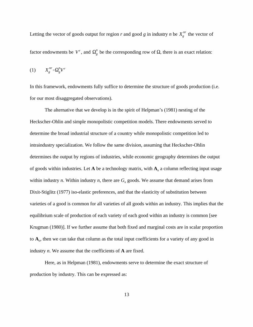
Letting the vector of goods output for region r and good g in industry n be the vector of
factor endowments be , and be the corresponding row of S, there is an exact relation:
(1)
In this framework, endowments fully suffice to determine the structure of goods production (i.e.
for our most disaggregated observations).
The alternative that we develop is in the spirit of Helpman’s (1981) nesting of the
Heckscher-Ohlin and simple monopolistic competition models. There endowments served to
determine the broad industrial structure of a country while monopolistic competition led to
intraindustry specialization. We follow the same division, assuming that Heckscher-Ohlin
determines the output by regions of industries, while economic geography determines the output
of goods within industries. Let A be a technology matrix, with A a column reflecting input usagen
within industry n. Within industry n, there are G goods. We assume that demand arises fromn
Dixit-Stiglitz (1977) iso-elastic preferences, and that the elasticity of substitution between
varieties of a good is common for all varieties of all goods within an industry. This implies that the
equilibrium scale of production of each variety of each good within an industry is common [see
Krugman (1980)]. If we further assume that both fixed and marginal costs are in scalar proportion
to A , then we can take that column as the total input coefficients for a variety of any good inn
industry n. We assume that the coefficients of A are fixed.
Here, as in Helpman (1981), endowments serve to determine the exact structure of
production by industry. This can be expressed as:

X nr'3Gn
g'1X nr
g 'S̄nV r
S̄
14
(2) ,
where is an N x N matrix. However endowments provide no information about a region’s
production structure within an industry — viz. the goods composition of production within the
industry. For example, they tell us which regions have a large textile industry, but not whether this
will be occupied producing carpets, rugs, etc.
We now need to specify how the location of goods production within industries is
determined for the economic geography specification. Absent idiosyncratic components of
demand, regions will divide production across goods within an industry in the same proportion as
all other regions. Hence regions with a large industry n will produce absolutely large amounts of
all goods within n, but cet. par. will have the same composition across goods as regions with a
smaller industry n. This base level of production of a particular good for a region, which depends
on that region’s overall commitment to the encompassing industry and to the importance of that
good in the aggregate within that industry, is what we will refer to as SHARE.
However, in the spirit of Krugman (1980), we posit that this base level of production of a
good must be adjusted to reflect the influences of idiosyncratically high demand. Our specification
is influenced by Weder (1995) to focus on differences in the relative importance of a good for the
specific region relative to all the regions taken together. The magnitude of this influence is, of
course, also influenced by that region’s total commitment of resources to the industry of interest.
This will give rise to a variable that we term IDIODEM. This will play a key role when we turn to

(nrg /
X nrg
X nr*nr
g /D nr
g
D nr
X nrg 'f (nROJ
g X nr, *nrg & *nROJ
g X nr
X nrg
X nr
X nrg ' "n
g % $1 (nROJg X nr % $2 *nr
g & *nROJg X nr % ,nr
g
X nrg ' "n
g % $1 SHARE nrg % $2 IDIODEM nr
g % ,nrg
15
hypothesis testing, since the economic geography framework predicts that the responsiveness of
goods production to movements in IDIODEM will be more than one-to-one.
We can state this hypothesis first in a general form. Let , , and ROJ
stand for the rest of Japan (except region r). Then goods production is modeled as:
(3)
where D denotes absorption in either the region, r, or Japan as a whole, J, and the first derivatives
are expected to be non-negative. The first term in f captures the tendency for each region to
produce the same relative shares of each good as other regions. Specifically, we postulate that a
region’s output of any good, , is going to be centered around the product of: (a) The share of
that good in that industry’s output for the rest of Japan; and (b) A scale term reflecting that
industry’s total size within the region, . The second term in f measures the demand deviation.
If all regions demanded the same share of each good, this term would equal zero. If a good
comprises a greater (smaller) share of demand within an industry, however, this term will be
positive (negative) indicating that the region is an idiosyncratically high (low) demander of that
good. Again this is scaled by region r’s output in industry n.
We will estimate a linear of version of (4) presented below:
(4)
or equivalently
(4N)

X nrg ' "n
g % $1 SHARE nrg % $2 IDIODEM nr
g % Sng V r % ,nr
g
The fact that the home market effect distinguishes the theory only when there exist costs5
of trade is of little practical import. It is true that, for simplicity, the theoretical literature in both
16
While we believe this exercise is informative, we do not want to stop with estimation of
equation (4N). The reason is that such a specification may suffer from an omitted variables bias, as
it assumes that endowments play no role in the location of goods production once we know the
level of industry output. Thus we estimate a nested model:
(4") ,
We want to verify that the conclusions derived from our earlier tests are robust to allowing
endowments to matter for output at a finer level of production. The structure that we have placed
on the analysis enables us to directly test the hypothesis of whether economic geography can
improve our understanding of production patterns at the goods level relative to the hypothesis
that all production is determined by endowments.
A few more words are in order about the specification. If the production of goods within a
region is proportional to production of these goods in the rest of Japan, then SHARE will equal
the expected level of production of a good given output at the industry level. In the specification
without endowments, one should expect the coefficient on SHARE to be unity.
Our main interest is in testing a null that Heckscher-Ohlin predicts the level of goods
output against an alternative that an augmented economic geography model does so. However, it
will prove informative to postpone this test and first consider directly several hypotheses
concerning equation (4"). The key is the interpretation of the coefficient ß , for which we2
distinguish three hypotheses. In a frictionless world (comparative advantage or IRS), the
geographical structure of demand should have no influence of production patterns, so ß = 0. In a25

frameworks has traditionally ignored costs of trade. This is relatively innocuous in the case ofcomparative advantage, much less so for increasing returns. In any case, we will see that our datastrongly reject the zero-trade-cost model, as is consistent with the recent work of McCallum(1995) and Engel and Rogers (1996).
17
comparative advantage world with trade costs, the geographical location of demand does matter.
But so long as import demand and export supply curves have the conventional slopes, the
response of local supply to idiosyncratic components of demand should be at most one-to-one.
Finally, as discussed previously, in the presence of economic geography, we expect the response
of local production to idiosyncratic components of demand to be more than one-to-one.
Summarizing:
Interpretation of ß2
1) ß = 0: Frictionless World (Comparative Advantage or IRS)2
2) ß 0 (0, 1]: Comparative Advantage with Trade Costs2
3) ß > 1: Economic Geography2
3 Empirics
3.1 Econometric Issues
Equations (2) and (4N) can be estimated at various levels of aggregation, separately or as a
system of seemingly unrelated regressions. The latter yields maximum power to discern the
average impact of economic geography in our sample. Alternatively, we can allow the coefficients
on the parameters to vary at the goods or industry level.
Direct estimation of (4N) is not possible because of a simultaneity problem. Because X isgnr
an element of X one cannot treat them as independent observations. Davis and Weinstein (1996)nr

var ,nrg ' Nn
g GDP2n
g
r
18
show however, that if we assume that factor endowments drive aggregate production, then we
will have a theoretically consistent set of instruments: factor endowments. In what follows, we
therefore always instrument X on factor endowments.nr
Second, there are two types of heteroskedasticity in these data. Errors are likely to be
correlated with the size of both regions and industries. These two types of heteroskedasticity can
be corrected for by postulating that for each good the error process is of the form given below:
(5)
where N and 2 are parameters. We corrected for heteroskedasticity by first estimating theg gn n
system and generating the squared residuals. Following Leamer (1984), We then regressed the
log of this series on the log of regional GDP and then used the fitted values to form our weighting
series for the heteroskedasticity correction.
3.2 Data Issues
In this section we provide an overview of the data used in the paper (details on the
construction of variables are in the appendix). Our data set contains output, endowment, and
absorption data for the 47 prefectures/cities of Japan. However, we were concerned that people
in the cities of Tokyo and Osaka might be working in the city but living and consuming in an
adjacent prefecture, so we were forced to aggregate some of the data. We formed two
aggregates: Kanto, out of the city of Tokyo and the prefectures of Yamanashi, Kanagawa, Chiba,
and Saitama; and Kinki, out of the prefectures/cities of Hyogo, Kyoto, Nara, and Osaka. This

19
reduced our sample to 40 observations, but enabled us to significantly increase the probability that
anyone within a region consumed largely within that region.
Our next problem was how to define industries and goods. Ideally, we would like to rely
on industry classifications based on technological criteria rather than substitutability in demand.
Unfortunately, industry classification schemes are typically based upon the latter more than the
former. There is some evidence that standard industry definitions do contain information about
production technologies [Maskus (1991)]. However, since we had access to the Japanese
technology matrix, we decided that we could provide more theoretically sensible classifications
than those typically found in statistical annuals.
In earlier work [Davis, Weinstein, et al. (1997)] we had constructed a technology matrix
for Japan. This matrix enabled us to have direct information on college, non-college, and capital
usage for 30 sectors. Of these 30 sectors, we dropped eight non-tradable goods sectors and two
agricultural sectors (agriculture, forest, and fishery products and processed foods). We felt it
necessary to drop the agricultural sectors because large-scale Japanese industrial policy
interventions, such as price supports, marketing boards, tax breaks, subsidies, zoning laws, etc.
significantly distort demand and supply in these sectors. Indeed, this accounts for the fact that in
our data 13 per cent of private land in the city of Tokyo (i.e. not the greater Tokyo metropolitan
area) is farmland. Finally we also dropped mining since it is obviously an endowment-based
sector.
The nineteen sectors that we eventually used are reported in Table 1. Davis and Weinstein
(1996) argued that in international data one can reject the economic geography specification in
favor of the Heckscher-Ohlin specification for these industry categories. However, as we have

20
suggested earlier, there is reason to be more optimistic that we can identify home market effects in
Japanese data. Bernstein and Weinstein (1997) argue that the reason for the good fits in
international data is the interaction between transaction costs and Heckscher-Ohlin effects. These
authors demonstrate that on Japanese data, where transactions costs are small, there is substantial
production indeterminacy at this level of aggregation. This has two important implications for our
work. First, since endowments do not predict output as well on regional data as on international
data, there is more latitude for other factors, such as economic geography, to determine regional
production. Second, the fact that transportation costs are substantially smaller between regions
means that the observed economic geography effects will be stronger [cf. Krugman (1991)]. Both
of these reasons suggest that we should be more optimistic about finding a role for economic
geography in determining regional production.
In some of the exercises that we will carry out, aggregation of goods into industries may
in principle matter a great deal. The theory literally holds that all varieties of all goods within an
industry use common input coefficients. Obviously this is too much to hope for with real data. So
we are required to aggregate the goods into industries in a way that respects the underlying
theoretical requirement that goods within an industry use similar input coefficients. Unfortunately,
in a world with more than two inputs, there is no theoretically compelling manner for performing
this aggregation. Hence we took a pragmatic approach of considering aggregation based on
factor-intensity ratios, taking two factors at a time. Unfortunately, although ranking sectors by
college to non-college ratios and capital to non-college ratios yields similar orderings, one obtains
radically different orderings if one looks at capital to college ratios. Ultimately, we decided to
form industry aggregates on the basis of college to non-college factor ratios, because this scheme

21
yielded the most plausible aggregates. The other aggregations schemes, especially the capital to
college scheme, had enormous outliers and produced very odd mixes of industries.
We calculated the ratio of college to non-college workers in each sector and then divided
the 19 goods into six industry aggregates based on the similarity of these ratios. The last columns
of Table 1 present these aggregates. Larger numbers indicate an industry composed of goods with
higher factor-intensity ratios. The commodity groupings for the college/non-college aggregation
scheme seem quite sensible, although there are a few anomalies, e.g. leather in industry 5.
Table 2 presents sample statistics for our data set using the college/non-college
aggregation scheme. These reveal that the typical good constitutes about one-third of the typical
industry and that there is substantial variation in idiosyncratic demand, which is important because
we need variation in the latter to drive the home market effects.
3.3 Estimating the Heckscher-Ohlin Production Model
Since our theoretical framework requires us to find a level of aggregation for which factor
endowments drive aggregate production, it is reasonable to ask whether our aggregation scheme
enables us to explain much of the variance at the three-digit level. Table 3 presents results of
estimating equation (1) for our sample of 40 regions. What is striking in our results is the fact
that fits of the regressions are quite high. Indeed, our results indicate that, on average, factor
endowments can explain almost 80 per cent (0.786) of the variation of our aggregates.
It is worth remembering, however, that there are two sources of variation in these data.
One source is pure size-based variation: larger regions produce more output. If all of our
explanatory power came from this source of variation, it would be somewhat disturbing, since one

22
would like to believe that endowments should tell us something about the relative sizes of
industries within regions. In other words, we would like endowments to also tell us about cross-
sectional variation within regions of similar size. One way to eliminate this size-based variation
and examine the cross-sectional variation is to force the exponent on GDP to equal two in our
heteroskedasticity correction. This is equivalent to estimating a version of equation (2) in which
both sides have been deflated by GDP. When we estimated this version of the equation we
obtained an average R of 0.4. This suggests that even after controlling for size based variation,2
endowments explain almost half of the variance of aggregate output. Furthermore, our data
revealed that endowments had a more difficult time explaining more disaggregated output levels.
Using the same specification, we only obtained an average R of only 0.3 when we ran the same2
specification on the most disaggregated data. This is consistent with the theoretical notion that
the Heckscher-Ohlin framework performs better using aggregates of industries with similar factor
intensities than using disaggregated data.
Overall, our results suggest that endowments and output are highly correlated on regional
data, and we have therefore established that the idea that endowments matter in determining the
location of production is a credible null hypothesis.
3.4 Testing for Home Market Effects
Before presenting our regression evidence, we begin by plotting our data. Our
formulation of the theory, given in equation (4"), suggests that we have a multivariate relationship
between the variables. If , however, we impose that ß equals 1, divide through by industry level1
output, and carry the SHARE variable over to the left-hand side, we obtain

(nrg & (nJ
g '"n
g
X nr% $2 *nr
g & *nJg % ,̃nr
g
23
.
The left-hand side of this equation measures how the share of industry output within a prefecture
deviates from that share for the rest of Japan, while the term in parentheses indicates the deviation
in absorption. In Figure 1 we refer to these two variables as the "Production Deviation" and the
"Absorption Deviation."
If economic geography has some role to play in these data one should expect to see
absorption deviations produce more than one-for-one movements in output. This would result in
a line with a slope of more than one. On the other hand if comparative advantage determined
production, then one would expect to see a line with a slope of less than one. As we see in Figure
1, the slope of the fitted line is 1.7. This suggests economic geography effects. Based on the slope
of the fitted line in this figure, a rise in a prefecture of idiosyncratic demand leads net exports to
rise by 70 per cent of the increment to local demand.
These results are surprising in light of our earlier work on international data. We
conducted a similar experiment for the OECD using 2- and 3-digit ISIC classifications (which
approximately correspond to the level of aggregation here). In the international data, the fitted
line was significantly below the diagonal at this level of aggregation, with a slope of only 0.66. In
other words, international data revealed no economic geography effect at this level of
aggregation, and only a very weak relationship at greater levels of disaggregation.
Although this graph is quite suggestive that economic geography might matter for regional
specialization, regression analysis will allow us to examine these relations more precisely. We
begin by estimating equation (4N). The results from this exercise are presented in Table 4. When

The coefficient on SHARE typically was negative in specifications with endowments. 6
This is largely due to the high degree of multicollinearity between this variable and theendowments. Since SHARE simply picks up industry size effects that can easily be captured byendowments, we experimented with omitting the variable and constraining it to equal one. Theseexperiments did not qualitatively alter our results.
24
we do not include factor endowments in the specification, our econometric results confirm the
general impression of the data that we obtained in Figure 1. Although the coefficient is slightly
smaller, its value of 1.42 is clearly in the range of economic geography.
The results presented thus far have examined economic geography against a very weak
null hypothesis: viz. that factor endowments do not matter at all at the goods level. Davis and
Weinstein (1996), however, show that factor endowments play an important role in determining
production at this level of aggregation on international data. This suggests that by leaving out
factor endowments from our estimating equations we may be creating an omitted-variables bias.
Consider the following possibility. We know that an important component of absorption is
demand for intermediate goods. Demand for intermediates is determined by the production of
final goods, but, if one believes in equation (1), production of the latter is driven by endowments.
This implies that demand for intermediates may be driven by endowments. In other words, if one
believes that endowments determine production, then it would not be surprising to find that there
is a correlation between production and absorption because both are driven by endowments.
The obvious solution is to estimate equation (4") since it includes factor endowments on
the right-hand side. The results of this exercise are presented in the second column of Table 4.
Interestingly, this causes the coefficient on IDIODEM to decline to 0.9. This implies that once6
we account for factor endowments, it no longer is the case that movements in demand produce

25
more than proportionate movements in production. In other words, this specification rejects
economic geography.
This result is troubling, especially in light of our earlier work. On international data, we
also rejected the economic geography specification, but when we did so in the specification with
factor endowments, we obtained a coefficient on IDIODEM of 0.3. This implies that in
international data, on average less than one-third of any deviation in demand was met by higher
domestic production, the rest being met by imports. This result makes sense in light of the
existence of international transaction costs which theoretically can cause demand and production
to covary. What is more puzzling is that if one believes that comparative advantage drives
production then one should also believe that in regional data, where transportation costs are
presumably lower, one should obtain an even smaller coefficient on IDIODEM. Instead we have
a coefficient that is too large to plausibly be generated by comparative advantage and transport
costs, but too small to signal economic geography.
One explanation for these results is that not all sectors are composed of monopolistically-
competitive industries. Suppose that only a few of our aggregates actually contain sectors
exhibiting increasing returns. Then our system of equations would be pooling together industries
in which the coefficient on IDIODEM is greater than unity with sectors in which the coefficient is
less than unity. This pooling could be the explanation for a coefficient that is too high to plausibly
describe a comparative advantage world, but too low to lead us to believe that economic
geography matters.
Fortunately, it is straightforward to modify our theory to address this problem. Assume
that some of our aggregates are composed entirely of constant returns to scale sectors and others

26
of increasing returns to scale sectors. Then the correct test would be to run equation (4O)
separately for each aggregate. This should result in aggregates without monopolistically-
competitive sectors exhibiting low coefficients on IDIODEM, but sectors with increasing returns
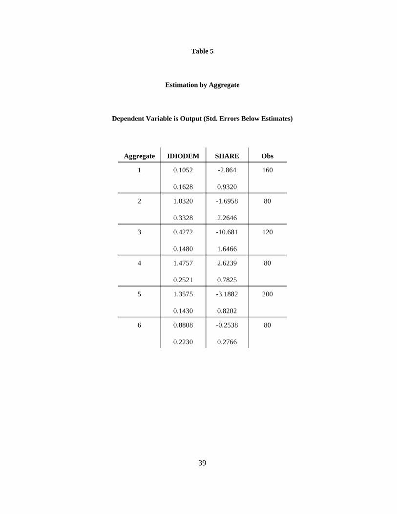
producing coefficients over unity. The results from this exercise are presented in Table 5. In the
three least skilled-intensive aggregates, we detect no significant economic geography effect.
However, in the more skill-intensive aggregates 4 and 5 we find a coefficient that is larger than
unity and significant at the 10 and 5 per cent levels respectively. The fact that these sectors
contain such plausible economic geography candidates as general machinery, electrical machinery,
transportation equipment, and precision instruments makes it even more believable that economic
geography effects may be present in these data.
However, it is also important to focus on economic, not only statistical, significance.
While we have been able to detect the presence of economic geography effects, it remains to be
seen whether it matters much for production. To assess the latter we consider ß-coefficients.
These statistics tell us how sensitive production is to movements in idiosyncratic demand.
Formally, a ß-coefficient tells us how many standard deviations the dependent variable is
predicted to move if the independent variable moves one standard deviation. As discussed by
Leamer (1984), these statistics are useful in answering questions regarding which independent
variables are important in determining movements in the dependent variable. In earlier work on
international data, we found that often even when we could detect economic geography in the
sample, this impact was economically small. While we find larger effects in the regional data, they
nonetheless remain modest. A one-standard-deviation movement in idiosyncratic demand moves
production by 0.22 standard deviations in aggregate 4, and by 0.09 standard deviations in

27
aggregate 5. In other words, knowing the variation in idiosyncratic demand does not provide
much information about the variation in production. Indeed, these numbers are not that different
than what we found on international data, suggesting that even in the sectors where economic
geography matters, the effects are relatively modest.
These results, however, are obviously very sensitive to the aggregation scheme. For
example, the inclusion of an unlikely economic geography candidate, leather, in aggregate 5 may
dilute the overall impact of economic geography in these data. In fact, while we found that
changing the basis of our aggregation scheme had little impact on estimates obtained in the full
system, changing the mix of goods within our industry definitions could cause different groups of
industries to be labeled as sectors with significant economic geography effects.
One solution to this theoretical and empirical mire is to foreswear aggregation altogether,
and allow all coefficients to vary at the goods level. This might be appropriate if, contrary to our
initial theoretical specification, the elasticity of substitution between varieties of a good is different
for the various goods within an industry. The results from this exercise are presented in Table 6.
The coefficient on IDIODEM is significantly larger than unity for eight of the nineteen sectors:
textiles, paper and pulp, iron and steel, chemicals, transportation equipment, precision
instruments, non-ferrous metals, and electrical machinery. With perhaps the exception of paper
and pulp, all of these seem like plausible candidates for monopolistic competition, with textiles,
transportation equipment, iron and steel, and electrical machinery providing canonical examples of
the power of the economic geography framework [see Krugman (1991)]. Furthermore, our
results are robust to whichever aggregation scheme we choose. The variables SHARE and
IDIODEM will vary depending on whether we group industries on the basis of college to non-

28
college, capital to non-college ratios, or capital to college ratios. However, we found that all of
these sectors except paper and pulp were identified as exhibiting economic geography effects
regardless of the aggregation scheme.
We can run an additional robustness check to confirm that we are identifying economic
geography effects here. We posit that the R&D-intensity of an industry may be used as a proxy
for the increasing returns and monopolistic competition that underlie the economic geography
theory. Figure 2 plots our estimated coefficients against sectoral R&D expenses divided by sales.
The correlation is 0.62, indicating that high R&D is associated with identification of economic
geography sectors. In fact, the four most R&D-intensive sectors are also the four sectors for
which we obtain the highest coefficients on IDIODEM.
Once again we confront the issue of economic significance. We repeat our experiment
with beta-coefficients, only this time we use the disaggregated results presented in Table 6. Table
7 reports the ß-coefficients for the 8 sectors for which we obtained statistically significant
economic geography coefficients. For these sectors, economic geography seems quite important.
A one standard deviation movement in idiosyncratic demand on average moves production by half
a standard deviation. In other words, observed fluctuations in idiosyncratic demand seem to
provide a lot of information about production patterns. Furthermore, in the important sector of
transportation equipment, these effects are very strong. Although economic geography may not
be that important for international specialization, there appears to be strong evidence that it
matters for certain sectors on a regional level.
4 Conclusion

29
This paper investigates the existence and importance of economic geography effects in
determining production structure for a sample of regions of Japan. Results from this regional
work both complement and contrast with those of Davis and Weinstein (1996) based on a sample
of OECD countries. Within the hypothesis testing framework developed, the earlier work found
scant support for the economic geography framework in the international sample. Moreover, even
insofar as it was possible to statistically identify such effects, their economic significance was very
minimal.
The regional data prove much more supportive of the economic geography hypothesis.
We find statistically significant effects of economic geography for eight of nineteen manufacturing
sectors: transportation equipment, iron and steel, electrical machinery, chemicals, precision
instruments, nonferrous metals, textiles, and paper and pulp. Moreover, for many of these sectors,
the economic geography effects are likewise very significant in economic terms.
Why are the regional effects of economic geography so strong, while the international
effects are so weak? We suspect two principal reasons. The first is trade costs: both transport
costs and myriad barriers to trade must surely be lower for trade between regions of a country
than between countries. In the economic geography framework, lower (but strictly positive) trade
costs lead to stronger effects, as this reflects lower implicit protection for production in the
relatively smaller markets. The second likely reason is the greater mobility of factors across
regions than countries. The suggestion is that such mobility will tend to reinforce the economic
geography effects, relieving scarcities in regions favorable on economic geography grounds for
production of particular goods.
30
How do these new results affect the conclusions of our earlier work regarding the
significance of economic geography in determining production specialization within the OECD?
They bring our earlier work into sharper focus in two respects. First, our earlier work had found
weak evidence of economic geography effects in as many as one-third of the goods that comprise
our sample. Since the microeconomic story that one tells at the regional and international level is
by and large the same, this strengthens our confidence that we had in fact identified economic
geography effects in the international data. The fact that we find the economic significance of
economic geography to be greater in the regional data is exactly what one would expect. This
likewise gives us greater confidence that our methodology is not inherently biased against finding
important economic geography effects. Hence it tends to strengthen our confidence in our earlier
finding that economic geography does not matter a great deal in understanding the structure of
international production.
The sharp contrast in the economic significance of economic geography effects across
regions versus internationally is a strong caution against accepting the view that the boundary
between international and interregional economics is on the verge of vanishing due to reductions
in border barriers. As such, this reinforces the perspective offered in McCallum (1995) and Engel
and Rogers (1996) that national borders continue to matter a great deal. Moreover, the strength
of the economic geography effects on the regional data suggest that the if the future holds a time
when international trade costs truly do fall to the level of interregional trade costs, then quite
substantial international restructuring of industry may be in the offing.
The empirical approach to identifying economic geography effects that we employ in this
paper is novel. In order to keep our framework simple, we have set to the side a large number of

31
important analytic and empirical questions. These include the roles of absolute market size,
forward- and backward-linkages, and “real-world” geography. Naturally, the results reported here
should be interpreted with an understanding that many issues in this area remain to be explored.
In sum, economic geography appears to be very important in determining the structure of
production across regions of Japan for eight of nineteen manufacturing sector. In contrast to
Davis and Weinstein (1996), which in exactly the same framework had shown scant economic
significance of economic geography for the structure of OECD production, here we find that it is
very important for the structure of regional production.

32
References
Armington, Paul S. (1969) “A Theory of Demand for Products Distinguished by Place ofProduction,” IMF Staff Papers, 16, March.
Ben-Zvi, Shmuel and Elhanan Helpman (1992) “Oligopoly in Segmented Markets,” in GeneGrossman, ed. Imperfect Competition and International Trade, Cambridge: MIT.
Bernhofen, Daniel (1995) “Intraindustry Trade and Strategic Interaction: Theory and Evidence,”mimeo, Clark University.
Bernstein, Jeffrey and David Weinstein (1997) “Do Endowments Predict the Location ofProduction? Evidence from National and International Data,” mimeo, University ofMichigan.
Bowen, Harry P., Edward Leamer, and Leo Sveikauskas (1987) “Multicountry, Multifactor Testsof the Factor Abundance Theory,” American Economic Review, v. 77.
Brander, James A. (1981) “Intra-Industry Trade in Identical Products,” Journal of InternationalEconomics, 11.
Chipman, John S. (1992) “Intra-Industry Trade, Factor Proportions and Aggregation,” inEconomic Theory and International Trade: Essays in Memoriam, J. Trout Rader, NY:Springer-Verlag.
Davis, Donald R. (1995) “Intra-Industry Trade: A Heckscher-Ohlin-Ricardo Approach,”, Journalof International Economics, 39:3-4, November.
Davis, Donald R. (1997) “Critical Evidence on Comparative Advantage? North-North Trade in aMultilateral World.” forthcoming Journal of Political Economy, October.
Davis, Donald R. and David E. Weinstein, (1996) “Does Economic Geography Matter forInternational Specialization,” NBER # 5706, August 1996.
Davis, Donald R., David E. Weinstein, Scott C. Bradford and Kazushige Shimpo (1997) “UsingInternational and Japanese Regional Data to Determine When the Factor AbundanceTheory of Trade Works,” American Economic Review, June.
Deardorff, Alan V. (1995) “Determinants of Bilateral Trade: Does Gravity Work in a NeoclassicalWorld?” forthcoming in Jeffrey Frankel, ed., Regionalization of the World Economy,Chicago: U. of Chicago and NBER.

33
Dixit, Avinash K., and Stiglitz, Joseph E. (1977) “Monopolistic Competition and OptimumProduct Diversity,” American Economic Review 67 (3), 297-308.
Engel, Charles and Rogers, John H. (1996) “How Wide is the Border?” American EconomicReview, December.
Helpman, Elhanan (1981) “International Trade in the Presence of Product Differentiation,Economies of Scale and Monopolistic Competition: A Chamberlin-Heckscher-OhlinApproach,” Journal of International Economics, 11:3.
Krugman, Paul (1979) “Increasing Returns, Monopolistic Competition, and Trade,” Journal ofInternational Economics, 9: 4.
Krugman, Paul R. (1980) “Scale Economies, Product Differentiation, and the Pattern of Trade,”American Economic Review, 70, 950-959.
Krugman, Paul R. (1984) “Import Protection as Export Promotion,” in H. Kierzkowski, ed.,Monopolistic Competition and International Trade, New York: Oxford U. Pr.
Krugman, Paul R. (1990) “Introduction,” Rethinking International Trade, Cambridge: MIT.
Krugman, Paul R. (1991) Geography and Trade, Cambridge: MIT.
Krugman, Paul R. (1994) “Empirical Evidence on the New Trade Theories: The Current State ofPlay,” in New Trade Theories: A Look at the Empirical Evidence, London: Center forEconomic Policy Research.
Krugman and Venables (1995) “Globalization and the Inequality of Nations,” Quarterly Journalof Economics, CX: 4.
Leamer, Edward (1984) Sources of International Comparative Advantage: Theory and Evidence,Cambridge: The MIT Press.
Linder, Staffan Burenstam (1961) An Essay on Trade and Transformation, NY: John Wiley andSons.
McCallum, John (1995) “National Borders Matter: Canada-US Regional Trade Patterns,”American Economic Review, 85:3.
Ricardo David (1951), “On the Principles of Political Economy and Taxation,” (The Works andCorrespondence of David Ricardo, vol. 1), ed. P. Sraffa, Cambridge: Cambridge U. Pr.

34
Rybczynski T.M. (1955) “Factor Endowments and Relative Commodity Prices,” Economica,XXII.
Weder, Rolf (1995) “Linking Absolute and Comparative Advantage to Intra-Industry TradeTheory,” Review of International Economics, 3:3, October.

35
Table 1
Aggregation Scheme
Sector College/Non- Capital/Non-College Capital/College
CollegeTextiles 1 1 4Apparel 1 1 2Lumber & Wood 1 1 5Furniture 1 1 3Ceramics, Stone, Clay, Glass 2 3 5Iron and Steel 2 5 6Paper and Pulp 3 4 5Rubber 3 3 4Fabricated Metal Products 3 2 3Transportation Equipment 4 4 5Other Manufacturing 4 3 4Leather & Leather Products 5 1 1Non-Ferrous Metals 5 4 5General Machinery 5 3 3Electrical Machinery 5 3 3Precision Instruments 5 2 2Printing and Publishing 6 2 2Chemicals 6 5 4Petroleum and Coal Products 6 6 6

36
Table 2
Variable Obs Mean Std. Dev. Min MaxSHARE/X 760 0.3158 0.2113 0.0108 0.7746nr
IDIODEM/X 760 0.0000 0.0824 -0.4037 0.4037nr
Non-College 40 1585633 2500886 372125 14500000College 40 426592 1063285 62628 6443185Capital 40 7559625 13400000 1469625 79100000Land 40 2034 2570 555 16487

37
Table 3
Aggregated Production on Factor Endowments
(40 Regions, Heteroskedasticity Corrected Estimates)
t-statistics F =.01,5,35
3.6
Constant College Non- Capital Land F-Statistic AdjustedCo Rllege
2
Aggregate 1 -0.343 -3.389 1.29 1.715 -3.823 14.77 0.5854
Aggregate 2 -1.208 -2.413 -0.085 2.432 -3.522 24.02 0.7024
Aggregate 3 -3.317 -2.286 3.255 0.266 -3.503 78.45 0.8882
Aggregate 4 -2.702 -1.758 1.213 1.209 -3.422 11.86 0.5268
Aggregate 5 -2.086 0.396 3.182 -0.946 -2.621 70.19 0.8765
Aggregate 6 0.467 4.994 1.323 -1.098 -0.534 1192.63 0.9919

38
Table 4
Seemingly Unrelated Regression Results
Dependent Variable is Production
IDIODEM 1.416 0.8880.025 .070
SHARE 1.033 -1.74410.007 0.211
FACTORS No Yes
Observations 760 760
(Standard errors are below estimates)
39
Table 5
Estimation by Aggregate
Dependent Variable is Output (Std. Errors Below Estimates)
Aggregate IDIODEM SHARE Obs
1 0.1052 -2.864 160
0.1628 0.9320
2 1.0320 -1.6958 80
0.3328 2.2646
3 0.4272 -10.681 120
0.1480 1.6466
4 1.4757 2.6239 80
0.2521 0.7825
5 1.3575 -3.1882 200
0.1430 0.8202
6 0.8808 -0.2538 80
0.2230 0.2766

40
Table 6
Disaggregated Estimation
Dependent Variable is Output (Std. Errs. Below estimates)
Industry IDIODEM SHARE Factors Adjusted R2 Observations
Textile 3.9532 0.5932 Yes 0.8468 40
0.4570 3.2302
Apparel -1.5866 -24.3909 Yes 0.5725 40
0.2843 4.3741
Lumber 1.0622 4.1937 Yes 0.8106 40
0.4440 1.8351
Furniture -0.5538 -5.1598 Yes 0.988 40
0.2765 1.4389
Pulp, paper 1.9913 -8.9731 Yes 0.8917 40
0.3150 1.7861
Printing 0.7269 -0.3423 Yes 0.9979 40
0.2296 0.2876
Chemicals 6.6781 0.9248 Yes 0.9928 40
1.2454 1.1038
Petrol, Coal -0.4655 -6.3220 Yes 0.9934 40products 2.3048 4.2047
Rubber -0.1081 -24.5223 Yes 0.8454 40
0.1763 5.78042
Leather, leather 0.1643 -7.1330 Yes 0.9412 40products 0.4053 1.7866

41
Stone, clay, -0.6454 -5.0674 Yes 0.7681 40glass
0.4148 2.4824
Iron, steel 3.9294 -3.9582 Yes 0.7663 40
0.5613 6.2968
Non-ferrous 1.5932 2.5509 Yes 0.962 40metals
0.1741 3.1334
Fabricated metal -0.8197 -14.0257 Yes 0.5972 40
1.0820 7.0734
General -0.4219 -4.4744 Yes 0.7802 40machinery 0.9524 2.6163
Electrical 6.2713 5.6614 Yes 0.9002 40machinery 1.3552 3.7628
Transport 6.7060 1.2685 Yes 0.8826 40equipment 0.5024 0.9336
Precision 4.32139 -3.9460 Yes 0.7477 40instruments 0.8115 1.8107
Other 0.0655 1.1179 Yes 0.5307 40manufacturing 0.3824 1.4888

42
Table 7
Beta Coefficients for Goods with Significant Coefficients on IDIODEM
Sector BetaCoefficient
Textiles 0.82Iron and Steel 0.40Paper and Pulp 0.51Transportation Equipment 0.74Non-Ferrous Metals 0.42Electrical Machinery 0.37Precision Instruments 0.42Chemicals 0.53

Ξ
Ξ
Ξ
Ξ
Ξ
Ξ
Ξ
Ξ
Ξ
Ξ
Ξ
Ξ
Ξ
Ξ
Ξ
Ξ
Ξ
Ξ
Ξ
Ξ
Ξ
Ξ
Ξ
Ξ
Ξ
Ξ
Ξ
Ξ
Ξ
Ξ
Ξ
Ξ
ΞΞ
Ξ
Ξ
Ξ
Ξ
Ξ
Ξ
Ξ
Ξ
Ξ
Ξ
Ξ
Ξ
Ξ
Ξ
Ξ
Ξ
Ξ Ξ
Ξ
Ξ
Ξ
Ξ
Ξ
Ξ
Ξ
Ξ
Ξ
Ξ
Ξ
Ξ
Ξ
ΞΞ ΞΞ Ξ
Ξ
Ξ
Ξ
Ξ
Ξ
Ξ
Ξ
Ξ
Ξ
Ξ
Ξ
Ξ
Ξ
Ξ
Ξ
Ξ
Ξ
Ξ
Ξ
Ξ
Ξ
Ξ
Ξ
Ξ
ΞΞ
ΞΞ
Ξ
Ξ
Ξ
Ξ
Ξ
Ξ
Ξ
Ξ
Ξ
Ξ
Ξ
Ξ
Ξ
Ξ
Ξ
Ξ
Ξ
ΞΞ
ΞΞ
Ξ
Ξ
Ξ
Ξ
Ξ
Ξ
Ξ
Ξ
Ξ
Ξ
Ξ
Ξ
Ξ
Ξ
Ξ
Ξ
Ξ
ΞΞ
Ξ
ΞΞ
ΞΞΞ
Ξ
Ξ
Ξ
Ξ
Ξ
Ξ
Ξ
Ξ
Ξ
Ξ
ΞΞ
Ξ
Ξ
Ξ
Ξ
Ξ
Ξ
Ξ
Ξ
Ξ
Ξ
Ξ
Ξ
Ξ
Ξ
Ξ
ΞΞ
Ξ
Ξ
Ξ
Ξ
Ξ
Ξ
ΞΞ
Ξ
ΞΞ
Ξ
Ξ
Ξ
Ξ
ΞΞ
Ξ
Ξ
Ξ
Ξ
Ξ
Ξ
Ξ
ΞΞΞ
Ξ
Ξ
Ξ
Ξ
Ξ
Ξ
ΞΞΞ
Ξ
Ξ
Ξ
Ξ
ΞΞ
Ξ Ξ
Ξ
ΞΞ
Ξ Ξ
Ξ
Ξ
Ξ
Ξ
Ξ
Ξ
Ξ
Ξ
Ξ
Ξ
ΞΞ
Ξ
ΞΞ
Ξ
Ξ
Ξ
Ξ
Ξ
Ξ
Ξ
Ξ
Ξ
ΞΞ
Ξ
Ξ
ΞΞ
Ξ
Ξ
Ξ
Ξ
Ξ
Ξ
Ξ
Ξ
Ξ
Ξ
Ξ
Ξ
Ξ
Ξ
Ξ
Ξ
Ξ
Ξ
Ξ
Ξ
Ξ
Ξ
Ξ
Ξ
Ξ
Ξ
Ξ Ξ
Ξ
Ξ
Ξ
Ξ
Ξ
Ξ
Ξ
Ξ
Ξ
Ξ
Ξ
Ξ
Ξ
Ξ
Ξ
Ξ
Ξ
Ξ
Ξ
Ξ
Ξ
Ξ
Ξ
Ξ
ΞΞ
Ξ
Ξ
ΞΞ
Ξ
Ξ
Ξ
Ξ
Ξ
Ξ
ΞΞ
ΞΞ
Ξ
Ξ
Ξ
ΞΞ
ΞΞ
Ξ
Ξ
Ξ
Ξ
ΞΞ
Ξ
Ξ
Ξ
Ξ
ΞΞ ΞΞ
Ξ
Ξ
Ξ
Ξ
Ξ
Ξ
Ξ
Ξ
Ξ Ξ
ΞΞ
ΞΞ
Ξ
Ξ
Ξ
Ξ
Ξ
Ξ
Ξ
Ξ
ΞΞ
Ξ
Ξ
Ξ
Ξ
Ξ
Ξ
Ξ
Ξ
Ξ
Ξ
Ξ
Ξ
Ξ
ΞΞ
Ξ
Ξ
Ξ
Ξ
ΞΞ
Ξ
Ξ
Ξ
Ξ
Ξ
Ξ
Ξ
Ξ
Ξ
Ξ
Ξ
Ξ
Ξ
Ξ
Ξ
Ξ
Ξ
Ξ
Ξ Ξ
Ξ
Ξ Ξ
Ξ
Ξ
Ξ
Ξ Ξ
Ξ
Ξ
Ξ
Ξ
Ξ
ΞΞΞ
Ξ
Ξ Ξ
Ξ
Ξ
Ξ
Ξ
Ξ
ΞΞ
Ξ
Ξ
Ξ
Ξ
Ξ
Ξ
Ξ
Ξ
Ξ
Ξ
Ξ
Ξ
ΞΞ
Ξ
Ξ
Ξ
Ξ
Ξ
Ξ
Ξ
Ξ
Ξ
Ξ
Ξ
Ξ
Ξ
Ξ
ΞΞ
Ξ
Ξ
Ξ
Ξ
Ξ
Ξ Ξ
Ξ
Ξ
ΞΞ
Ξ
Ξ
Ξ
Ξ
ΞΞ
Ξ
Ξ
Ξ
Ξ
Ξ
Ξ
Ξ
Ξ
Ξ
Ξ
Ξ
ΞΞ
Ξ
Ξ
Ξ
Ξ
ΞΞ
Ξ
Ξ
Ξ
Ξ
ΞΞ
Ξ
Ξ
ΞΞ
Ξ
Ξ
Ξ
Ξ
Ξ
Ξ
Ξ
Ξ
Ξ
Ξ
Ξ
Ξ
ΞΞ
ΞΞ Ξ
Ξ
Ξ
Ξ
Ξ
Ξ
Ξ
Ξ
Ξ
Ξ
ΞΞ
Ξ
Ξ
Ξ
Ξ
Ξ
Ξ
Ξ
Ξ
Ξ
Ξ
ΞΞ
Ξ
Ξ
Ξ
Ξ
Ξ
Ξ
Ξ Ξ
Ξ
Ξ
Ξ
Ξ
Ξ
Ξ
Ξ
Ξ
ΞΞ
Ξ
Ξ Ξ
Ξ
Ξ
Ξ
Ξ
Ξ
Ξ
Ξ
Ξ
Ξ
Ξ
Ξ
Ξ
Ξ
Ξ
Ξ
Ξ
Ξ
Ξ
ΞΞ
Ξ
Ξ
Ξ
Ξ
ΞΞ
Ξ Ξ
Ξ
Ξ
Ξ
Ξ
Ξ
Ξ
Ξ
Ξ
ΞΞ
Ξ
Ξ
Ξ
Ξ
Ξ
Ξ
Ξ
Ξ
Ξ
Ξ
Ξ
Ξ
Ξ
Ξ
Ξ
Ξ
Ξ
Ξ
ΞΞ
Ξ
Ξ
Ξ
ΞΞΞ
Ξ
Ξ
Ξ
Ξ
Ξ
Ξ
Ξ
Ξ
Ξ
Ξ
Ξ
Ξ
Ξ
Ξ
Ξ
ΞΞ
Ξ
Ξ
Ξ
Ξ
Ξ
Ξ
Ξ
Ξ
Ξ
Ξ
Ξ
Ξ
Ξ
Ξ
Ξ
Ξ
Ξ
Ξ
Ξ
Ξ
ΞΞ
Ξ
Ξ
Ξ
Ξ
Ξ
Ξ ΞΞ
Ξ
Ξ
ΞΞ
Ξ
Ξ
Ξ
ΞΞ
Ξ
Ξ
Ξ
ΞΞ
Ξ
Ξ
Ξ
Ξ
Ξ
ΞΞΞ
ΞΞ
Ξ
Ξ
Ξ
Ξ
Ξ
Ξ
Ξ
Ξ
Ξ
Ξ
Ξ
Ξ
Ξ
Ξ
Ξ
Ξ
Ξ
Ξ
ΞΞ
Ξ
Ξ
Ξ
Ξ
Ξ
Ξ
Ξ
Ξ
Ξ
Ξ
Ξ
Ξ
Ξ
Ξ
Ξ
Ξ
Ξ
Ξ
Ξ
Ξ
Ξ
Ξ
Ξ
Ξ
Ξ
Ξ
Ξ
Ξ
Ξ
Ξ
Ξ
Ξ
Ξ
Ξ
Ξ
Ξ
-0.8
-0.6
-0.4
-0.2
0
0.2
0.4
0.6
0.8
-0.8 -0.6 -0.4 -0.2 0 0.2 0.4 0.6 0.8Idiosyncratic Demand
45E Line
Fitted Line
43
Figure 1
Production Distortion vs. Absorption Distortion

Ξ
Ξ
Ξ
Ξ
Ξ
Ξ
Ξ
Ξ
Ξ
Ξ
Ξ
Ξ
Ξ
Ξ
Ξ
-1
0
1
2
3
4
5
6
7
-1 0 1 2 3 4 5 6 7R&D/Sales
44
Figure 2
Coefficient on IDIODEM vs. R&D Intensity

45
DATA APPENDIX
PREFECTURAL ENDOWMENTS
The numbers of workers by educational attainment were entered by prefecture directly from theEmployment Status Survey of 1987 (Shugyo Kozo Kihon Chosa Hokoku). The capital stockswere imputed from prefectural investment data. Japan’s yearly Annual Report on PrefecturalAccounts (Kenmin Keizai Keisan Nempo) give investment flows for each prefecture from 1975to 1985. These flows were used to impute capital stock levels for each prefecture in 1985, usingcapital goods price deflators from the Annual Report on National Accounts (Kokumin KeizaiKeisan Nempo) and a rate of depreciation of 0.133 (This was the same rate of depreciation usedby Bowen, Leamer, and Sveikauskas (1987)). Each year’s flow was deflated using a capitaldeflator from the National Accounts.
PREFECTURAL PRODUCTION
The gross output of 20 manufacturing sectors in each prefecture was taken from the JapaneseCensus of Manufactures for 1985. The gross output of 9 non-manufacturing sectors in eachprefecture was taken from the Prefectural Accounts for 1985. Finally, these totals were scaledso that the 47-prefectural total for each sector exactly matched the total Japanese output asreported in the 1985 Input-Output Table of Japan. Thus, in effect, the data from the Censusof Manufactures and from the Prefectural Accounts was used in order to distribute totalJapanese output for each sector across the 47 prefectures as accurately as possible.
TECHNOLOGY
Each element of the 3x29 technology matrix B was calculated by dividing Japanese total outputfor the 29 sectors into the number of each factor present in each sector. Most of the data oncollege and non-college workers in each sector came from the 1988 Wage Census (ChinginSensasu). There were some gaps in this data as follows: 1) There was no data for college andnon-college workers for agriculture, forestry, and fisheries or for government. These numberswere taken from the 1987 Employment Status Survey (Showa 63 Nen Shugyo Kozo KihonChosa Hokoku Chiiki Hen I II). 2) There was also no data for the petroleum/coal and leatherindustries. Total employment for each of these sectors was taken from the 1985 Census ofManufactures. The number of college workers per unit output for each was then imputed byassuming that petroleum/coal has the same fraction of college workers as the chemicals sectorand that leather has the same fraction as manufacturing overall. The capital stocks in each of the

46
30 sectors were imputed from investment numbers, using the Annual Report of the CorporationSurvey for non-manufacturing and the Census of Manufactures for manufacturing.
ABSORPTION
Intermediate input use in each region was calculated using the Japan 30x30 IO matrix for 1985. Thus, INPUT = AX , where INPUT is intermediate consumption in region r, A is the IOr r r
matrix, and X is gross output in region r. Both INPUT and X , therefore, are 30x1 vectors.r r r
The 47 INPUT vectors together form a 30x10 intermediate consumption matrix. It isr
important to note that one of our sectors in both A and X is producers of government services.r
Government absorption is therefore included in INPUT . r
The construction of the consumption data was quite complex. In 1984, the Japanesegovernment performed a detailed survey of Japanese consumption on the prefectural level, theNational Survey of Income and Expenditure, that broke Japanese household consumption upinto 65 categories. Unfortunately this data cannot be easily concorded into the 30 industrialCategories that we use in the paper. However the Economic Planning Agency does provide a30x42 bridging matrix which map the 42 consumption commodities that can easily be formedfrom the 56 consumption categories in the Family Income and Expenditure Survey for 1987into 30 core sectors corresponding to the Japanese IO table. Unfortunately this second sourceof data only reports information for ten Japanese regions. Since the 65 categories of theNational Survey of Income and Expenditure did not always correspond to the 56 categories ofthe Family Income and Expenditure Survey, we used the following procedure to developconsistent series. First, for most categories there was a perfect match between the two sources,so we used the National Survey of Income and Expenditure for entries wherever possible. Wethen used regional totals scaled by household income shares to fill in the gaps. Since we wereusing both 1984 and 1987 data all prefectural entries were scaled so that they matched theregional totals.
This data was then aggregated up to 42 categories, producing a 42x47 matrix of finalconsumption by region. The survey data was based, of course, on consumer prices, so the bridgematrix was specially constructed to translate the consumption expenditure into producer prices.Most of the difference between consumer and producer prices results from wholesale and retailmarkups and from transportation costs, so the mapping shifted portions of spending on eachfinal good into the wholesale/retail trade and transportation sectors, reflecting the fact that toconsume anything bought retail is to consume the wholesaling, retailing, and transportationservices which brought the product to the store. Without this adjustment, the data would have

47
greatly underestimated final consumption of wholesale/retail and transportation services andwould have shown each region exporting far more of these services than is plausible.
There are no investment figures broken down for 30 sectors and 47 prefectures, so thesenumbers were imputed using IO Table investment data. The IO Table breaks down investmentinto the 30 sectors for Japan as a whole. This vector was then distributed across regions, usingas weights each region’s share in total investment for Japan as a whole. Thus, INV =r
(TI /TI )INV , where INV is a 30x1 investment vector for region r, TI is the total investmentr J rJ r
for that region in 1985 (taken from the prefectural accounts), TI is Japan’s total investment forJ
1985, and INV is the 30x1 investment vector taken from the IO Table. These 10 INV’sr
therefore formed a 30x10 investment matrix. Business consumption was added to the data ina similar fashion. The data for all prefectures was then aggregated into 29 sectors to make itcompatible with our B matrix.
R&D Data
Research and Development data was taken from the Report on the Survey of Research andDevelpment.