Embed Size (px)
Citation preview

Economic History Association
Notes on the Social Saving ControversyAuthor(s): Robert William FogelSource: The Journal of Economic History, Vol. 39, No. 1, The Tasks of Economic History(Mar., 1979), pp. 1-54Published by: Cambridge University Press on behalf of the Economic History AssociationStable URL: http://www.jstor.org/stable/2118909 .Accessed: 09/05/2011 14:21
Your use of the JSTOR archive indicates your acceptance of JSTOR's Terms and Conditions of Use, available at .http://www.jstor.org/page/info/about/policies/terms.jsp. JSTOR's Terms and Conditions of Use provides, in part, that unlessyou have obtained prior permission, you may not download an entire issue of a journal or multiple copies of articles, and youmay use content in the JSTOR archive only for your personal, non-commercial use.
Please contact the publisher regarding any further use of this work. Publisher contact information may be obtained at .http://www.jstor.org/action/showPublisher?publisherCode=cup. .
Each copy of any part of a JSTOR transmission must contain the same copyright notice that appears on the screen or printedpage of such transmission.
JSTOR is a not-for-profit service that helps scholars, researchers, and students discover, use, and build upon a wide range ofcontent in a trusted digital archive. We use information technology and tools to increase productivity and facilitate new formsof scholarship. For more information about JSTOR, please contact [email protected].
Cambridge University Press and Economic History Association are collaborating with JSTOR to digitize,preserve and extend access to The Journal of Economic History.
http://www.jstor.org
THE JOURNAL OF ECONOMIC HISTORY
VOLUME XXXIX MARCH 1979 NUMBER 1
Notes on the Social Saving Controversy
ROBERT WILLIAM FOGEL
This paper explores a number of the unresolved issues posed by the debate on the social saving of railroads. The final section includes a brief summary of the main findings of the new economic history of transportation.
I T is now more than 17 years since the first discussion of the social sav- ing of railroads at a meeting of economic historians,' and more than 16
years since the first publication of a paper dealing with this question.2 The ensuing train of research has been substantial. Applications of the social saving approach and critiques of these applications have been set forth in at least a dozen books and in several score of journal articles and reviews. The debate, as Patrick O'Brien recently observed, has been both exciting and illuminating.3 Because of the rich interaction between the investiga-
The Journal of Economic History, Vol. XXXIX, No. 1 (March 1979). i The Economic History As- sociation. All rights reserved. ISSN 0022-0507.
The author is Professor of Economics and History at Harvard University, Since this paper is based on class lecture notes, his first debt is to students in more than a dozen classes whose insightful com- ments and criticisms shaped these notes. He also benefited from seminar discussions of earlier ver- sions of this paper at the London School of Economics, Essex, Glasgow, Cornell, Westfalische Wil- helms-Universitlt, the Catholic University of Louvain, Washington (Seattle), Berkeley, Monash, Australian National University, the Kyoto Summer Seminar (Doshisha University), Stanford, Johns Hopkins, Northwestern, Uppsala, and Oslo. Robert Margo, Charles Kahn, Harry Holzer, Kenneth Sokoloff, and Georgia Villaflor provided insightful assistance during the final phases of the research. John Coatsworth, Stanley L. Engerman, David H. Fischer, Albert Fishlow, Roderick Floud, Ephim Fogel, David Galenson, Knick Harley, Gary Hawke, Bradley Lewis, Peter McClelland, Donald McCloskey, Jacob Metzer, Patrick O'Brien, and G. N. von Tunzelmann commented on late drafts. Jeffrey G. Williamson provided data needed to replicate his simulations.
I The discussion was held at the first annual Cliometrics Conference, Purdue University, Decem- ber, 1960.
2 In this JOURNAL, 22 (June 1962), 163-97. 3 Much of the social saving literature is cited in the bibliography to Patrick O'Brien, The New Eco-
1
2 Fogel
tors and the critics, important aspects of the transportation revolution of the nineteenth century have been clarified.
In this paper I seek to explore a number of still unresolved issues that have been posed by the debate. The comments that follow are divided into four parts. The first part deals with the nature of the social saving model and the limits of its usefulness for historical analysis. The next part takes up an array of practical and conceptual issues that have been raised about the data and procedures actually employed by myself and other re- searchers in our various estimates of the social saving. The third part fo- cuses on the difficulties of attempting to pass from a social saving calcu- lation to warranted statements about the impact of railroads on the long- term pattern of a nation's economic growth. The final part includes a brief summary of the main findings of the new economic history of transporta- tion and emphasizes that, in retrospect, the line of continuity between the newer and older research is stronger than it at first appeared.
THE NATURE AND LIMITATIONS OF THE SOCIAL SAVING MODEL
I defined the social saving of railroads in any given year as the differ- ence between the actual cost of shipping goods in that year and the alter-
nomic History of Railways (London, 1977). To this listing one should add: John Coatsworth, "Growth Against Development: The Economic Impact of Railroads in Porfirian Mexico," mimeo 1976, which is a translation and revision of Crecimento contra desarrollo: El impacto economic de losferrocarriles en el porfiriato, 2 vols., Sepsetentas No. 271-72 (Mexico City, 1976). Jeffrey G. Williamson, Late Nineteenth-Century American Development: A General Equilibrium History (Cambridge, 1974), espe- cially ch. 9.; Jeffrey G. Williamson, "The Railroads and Midwestern Development, 1870-1890: A General Equilibrium History," in David C. Klingaman and Richard K. Vedder, Essays in Nineteenth Century Economic History (Athens, Ohio, 1975), ch. 11; G. N. von Tunzelmann, Steam Power and British Industrialization to 1860 (Oxford, 1978), chs. 3, 6, and 11; Wray Vamplew, "Nihilistic Impres- sions of British Railway History," in Donald N. McCloskey, ed., Essays on a Mature Economy: Brit- ain after 1840 (Princeton, 1971), ch. 10; Jan de Vries, "Barges and Capitalism: Passenger Transporta- tion in the Dutch Economy, 1632-1839," A. A. G. Bijdragen, 21 (1978), ch. 8; Donald N. McCloskey, "New Model History," Times Literary Supplement, December 12, 1975; Peter Temin, Causal Factors in American Economic Growth in the Nineteenth Century (London, 1975), ch. 5; C. H. Lee, The Quan- titative Approach to Economic History (London, 1977), ch. 4; and Jon Elster, Logic and Society: Con- tradictions and Possible Worlds (Chichester, 1978), ch. 6. This supplement to O'Brien's list is far from exhaustive. In addition to other relevant works that are cited below, there are numerous interesting reviews and brief commentaries, especially in essays analyzing the methodology of the New Eco- nomic History. Some of these are listed in Peter D. McClelland, Causal Explanation and Model Build- ing in History, Economics, and the New Economic History (Ithaca, 1975).
Social saving calculations did not originate with present-day economists and economic historians. Such calculations were carried out by legislators and men of affairs who were involved in the decision processes on government aid for internal improvements during the nineteenth century, not only in America, but also in Europe. Albert Fishlow cites two early social saving estimates in American Rail- roads and the Transformation of the Antebellum Economy (Cambridge, 1965). Richard H. Tilly called my attention to an essay by Ernst Engel (the Prussian statistician identified with "Engel's Law") which presents a calculation of the social saving attributable to German railroads during 1840-80. Ernst Engel, "Das Zeitalter des Dampfes in technisch-statistischer Beleuchtung", Zeitschrift des Ko- niglichen Preussischen Statistischen Bureaus, (Berlin, 1880). Richard Hodne in his An Economic His- tory of Norway 1815-1970 (Tapir, 1975), p. 221, cites a study of the social saving of railroads in Nor- way by E. 0. J. Svan0e that appeared in Statsokonomisk Tidsskrift in 1887.

Presidential Address 3
native cost of shipping exactly the same bundle of goods between exactly the same points without the railroad. The second and third chapters of Railroads and American Economic Growth dealt with the estimation of this cost differential in the transportation of agricultural products for 1890. Because my formulation of the social saving model was verbal rather than algebraic, there has been some confusion regarding certain aspects of the model. The deficiency can be remedied by specifying a two-sector model in which the activities of one of the sectors, transportation, can be carried out under either of two production functions.4 Thus,
QA= a(La, Ka, QTa) (1)
QT = w(Lw, Kw) (2)
QT= r(Lr, Kr). (3)
(See Table I for the definitions of symbols.) The r process is superior to w so that the fixed quantity of transporta-
tion, QT, can be produced under r with less labor and capital than under w. In other words,
Lw =Lr+AL (4)
Kw = Kr + AK. (5)
Now, national income under the r function is QA + QTC where QTC
(which equals QT - QTa) is assumed fixed, as is QTa. Substitution of the w for the r function, keeping QT constant, will require the transfer of AL and AK from the production of all other things. Then national income (Y) will be
Y = QA' + QTC, where (6)
QA = a(La - AL, Ka - AK, QTa). (7)
It follows that the social saving is also the loss in national income caused by the substitution of an inferior for a superior transportation technology (or the gain in going from the inferior to the superior tech- nology), which is given by
(QA + QTC) - (QA' + QTC) = QA - QA' A L AL + aK A K, (8)
and which may be expressed in value terms as
(QA L+QAK
dL 3K JA P~(QA - QA')PA. (9)
4The model which follows differs from that presented in Robert W. Fogel and Stanley L. Enger- man, eds., The Reinterpretation of American Economic History (New York, 1971), p. 101, by allowing part of the output of the transportation sector to be purchased for use in the production of other out- put.

4 Fogel
TABLE I
DEFINITIONS OF PRINCIPAL SYMBOLS IN EQUATIONS AND DIAGRAMS
QT = output of transportation QT. - the part of QT used to produce Q. QTC QT - QTa transportation purchased as a final product QA - output of the all-other-things sector
L = labor K - capital
AL, AK = labor and capital shifted from the all-other-things sector a = the all-other-things function and inputs into it w = the inferior transportation function and inputs into it r = the superior transportation function and inputs into it
Y = national income PA - price of QA in the terminal period (that is, with railroads) D - intercept of the demand function for transportation P price of transportation e - elasticity of demand
St social saving estimated on the true value of e
So0 social saving estimated on the assumption - 0 Pw = price of transportation in a non-railroad world, if price - marginal cost Pw' = price of transportation in a non-railroad world, if price > marginal cost
Pr = price of transportation in a railroad world ho PW/Pr B = bias in the social saving caused by setting e = 0 i= social rate of return on the investment in railroads
_d = distance in (statute miles) or pence, depending on the context Rw - steamboat rate per ton-mile on wheat on the upper Mississippi
MR = marginal revenue MC = marginal cost
Qr = output of transportation in a railroad world Qw= output of transportation in a non-railroad world, if price marginal cost QW= output of transportation in a non-railroad world, if price > marginal cost Cc = construction cost of a canal (book value in 1889) CO = annual operating cost of a canal in constant dollars
Xp= cross-section of a canal prism in square feet XI = length of a canal in statute miles Xr = total rise and fall of a canal in feet Xf= annual tonnage of freight carried by a canal
X =- annual ton-miles of freight on the New York canals Xd = average distance of a haul on the New York canals during a year
X:w a dummy representing the Civil War years Qg = quantity of eastbound wheat, corn, and oats shipped by lake from Chicago, in tons M = quantity of wheat, corn, and oats produced nationally (in tons); a market-size variable Rr Chicago to Buffalo rate on wheat by railroad, in constant dollars RW = Chicago to Buffalo rate on wheat by lake (including Buffalo elevating changes) in constant
dollars B. = an index of the average size of grain-carrying lake vessels
N = annual length of the season of navigation Kb an index of the capital stock of grain-carrying lake vessels Q= the output of an industry benefiting from railroad-induced economies of scale in year i C, the cost of producing Q p= a vector of the prices of the inputs used to produce Q, x = the scale coefficient (the sum of the output elasticities in the industry-wide production
function) for an industry benefiting from railroad-induced economies of scale a "cap" over a variable designates the natural logarithm of that variable

Presidential Address 5
Interpretation of the Model
Several points should be noted about this model. First, the model does not purport to be, and is not, a complete or literal description of either the American or any other late nineteenth-century economy. It is a model de- signed to set an upper bound on the resource saving brought about by an improvement in transportation technology. The model produces an upper bound by setting the elasticity of demand (E) at zero and thereby fixi g the volume of transportation at the level observed with the superior (cheaper) form of transportation. If the elasticity of demand is allowed to be greater than zero, the rise in the cost of transportation would reduce the quantity of transportation purchased and hence also reduce the diver- sion of resources from the all-other-things sector to the transportation sec- tor (that is, it would reduce AL and AK).
Second, the increase in the cost of transportation is identically equal to the decrease in national income. This identity is brought about by the as- sumptions that the demand for transportation is perfectly inelastic, and that AL and AK come from resources previously employed in the produc- tion of QA rather than from previously unemployed resources.
Third, the model is not designed to deal with other important issues such as the effect of transportation improvements on the spatial location of economic activity, induced changes in the industrial mix of products within the all-other-things sector, induced changes in the aggregate sav- ings rate, and possible effects on either the rate of technological change in various industries or on the overall supplies of inputs. In order to take up such issues the model would have to be expanded considerably. The elas- ticities of demand and supply in each sector would have to be specified and estimated, and the number of sectors would have to be increased to permit analysis of the effect of transport changes on the geographic loca- tion of production and the redistribution of inputs among industries. A savings function would have to be specified, estimated, and so on. These are worthy enterprises, but they are also difficult. So far, only Jeffrey G. Williamson and Bradley G. Lewis have responded to the challenge in a substantial way.5
It should be clear, then, that the social saving is not a description of what actually happened but an answer to a hypothetical problem, a prob- lem similar in nature to those that engineers must solve successfully to build bridges and to those that manufacturers must confront in choosing between alternative machine designs. This answer rests on a detailed ex- amination of actual economic and technological characteristics of the al- ternative modes of transportation in historical context. The solution of the
s The Williamson model is discussed in the third section of this paper. Lewis, in a dissertation un- der way at the University of Chicago, is investigating the effect of railroads on the location of eco- nomic activity and other consequences stemming from the impact of railroads on relative prices.

6 Fogel
problem illuminates actual history not only because it provides a measure of the primary (cost-reducing or resource-saving) effect of railroads in the provision of a specified volume of transportation service, but also because it brings together a great deal of relevant information regarding actual ex- perience and systematically assesses the implications of this information. To carry out his computation of the social saving of U.S. railroads in 1859, Albert Fishlow, for example, not only had to delve into the differen- tial cost of transportation provided by railroads, waterways, and wagons for both passengers and freight but also had to determine how these dif- ferentials varied for specific categories of freight and passengers over a va- riety of routes and at different points in time. His analysis indicated that by 1859 railroad passenger transportation yielded direct benefits that were less than half of those yielded by the carrying of freight. Even more sur- prising and informative was his discovery that the great trunk lines ac- counted for just 8 percent of the social saving of railroads. Fishlow's anal- ysis showed that the trunk lines were constructed along routes where waterways were rather good substitutes for railroads. It was in the interior of the country where wagons or coaches were often the most feasible sub- stitutes that the social saving of railroads was greatest, accounting in Fish- low's calculation for nearly two thirds of the total.6r
The social saving model defines the r function on the basis of the rail- road technology at its most efficient aggregate level during the period un- der study, that is, by the aggregate technology prevailing at the end of the period. There is, however, no specification of how the w function should be defined. Fishlow defined the w function on the aggregate level of wa- terway and wagon technology actually in operation at the end of the pe- riod. In my book, I defined three plausible w functions and carried out so- cial saving calculations for each. The first calculation was based on canals that had actually been constructed by 1890; the second allowed for an ad- ditional 5,000 miles of canals that very likely would have been con- structed in the absence of railroads; the third adjusted the social saving for plausible improvements in wagon roads (such as surfacing).7 It should be noted that these successive characterizations of the w function do not pur- port to represent actual shifts in that function over time but are merely a set of plausible alternative characterizations of the production function for transportation in the absence of railroads.
Which is the "right" specification of the w function? There is no single "right" specification, but rather a fairly large set of alternative specifica- tions for which a social saving calculation can usefully be performed. The more detailed the set of specifications, the brighter the light that will be shed on the economic potential of alternatives to railroads, alternatives that were thwarted by the investment in railroads. These alternatives pro- vide fine tuning on the magnitude of the incremental benefits of railroads
'Alber Fishlow, American Railroads, p. 93. ' Robert W. Fogel, Railroads andAmerican Economic Growth: Essays in Econometric History (Balti-
more, 1964), ch. 3.

Presidential Address 7
as well as a means of decomposing the overall figure. Alternative specifi- cations also permit the historian, with his advantage of hindsight, to be able to identify errors made by planners and investors in the past because certain of their assumptions regarding future technological or market de- velopments turned out to be wrong. For example, the set of decisions that led to a 94 percent increase in the density of the U.S. railroad networks between 1890 and 1914 were based, to an extent that has yet to be eval- uated, on a failure to take adequate account of the rate of improvement in motor vehicles. If the speed of advance in motor transportation had been known, some of the extensions of railroads would not have taken place. Economic historians can now engage in categories of project evaluation that the engineers and planners of the 1890s could not entertain. Histori- cal hindsight makes it possible to determine which part of the increment to the railroad network after 1890 (or even before that date) should not have been built, as well as the extent to which the rate of improvement in common roads should have been accelerated.
Fishlow's calculation of the social saving was not made more realistic, as some have argued, by his assumption that in the absence of railroads waterways would have been limited to those actually in use in 1860. That is the least plausible of all possibilities. There can be little doubt that the relatively high prices of agricultural products in the North Atlantic states and in Europe would have made the extension of the canal system into the North Central states a highly profitable investment.8 But given the high cost of investigating this possibility, and considering the other issues to which he gave priority, Fishlow's decision not to pursue this matter made sense. Although his assumption yielded, not a least upper bound for the social saving but a relatively high upper bound, such a bound was quite adequate for the analytical issues he set out to address. The choice as to how far one ought to pursue calculations of the social saving on plausible alternative characterizations of the w function depends not only on the quality of the available data and on the cost of the investigation, but also on the research priorities that an investigator assigns to the array of issues that might be pursued.
That the authors of the major studies of the social saving of railroads often struck out in widely different directions should cause neither sur- prise nor consternation. We are richer, not poorer, because Fishlow tested the Schumpeter hypothesis of construction ahead of demand, because Ja- cob Metzer investigated the impact of railroads on the national unifica- tion of the Russian grain market, because Gary R. Hawke probed so in-
8 Cf. Fogel, Railroads, pp. 92-107. David has pointed out that the reduction in the /B estimate of the social saving due to the extension by 5,000 miles of the canal system implies a social rate of return on the investment in excess of 50 percent per annum. Paul A. David, "Transportation Innovations and Economic Growth: Professor Fogel On and Off the Rails," Economic History Review, 2nd Ser., 22 (Dec. 1969), 506-25, rpt. as ch. 6 of Paul A. David, Technical Choice, Innovation, and Economic Growth (Cambridge, 1975), pp. 291-314.

8 Fogel
sightfully into railway pricing policy, and because John Coatsworth demonstrated the intimate connection between railroad construction and the concentration of land ownership in Mexico.
A Technological Definition of the Social Saving
One of the most interesting questions related to the social saving model was raised by Stanley Lebergott, who focused not on the w function but on the r function. Lebergott argued that the social saving calculation should not be based on the observed railroad rate at the end of the period under investigation, or even on that rate adjusted for monopoly profit, but on the rate that would have prevailed if the railroad system had operated at the minimum point of its long-run supply function.
Figure 1 depicts the long-run supply function suggested by Lebergott. The quantity of freight service supplied is measured by tons of freight car- ried per mile of railroad track. Lebergott's argument rests on the quite plausible assumption that the supply price dropped continuously with the intensity of track utilization, up to some point, and then rose. Although Lebergott did not know at what intensity of track utilization this mini- mum was reached, he suggested that for the antebellum era it could prob- ably be represented by the data of the Philadelphia and Reading Rail road. During the 1850s this company hauled about 25,000 tons per mile of track per year. Lebergott estimated that at such intensities of road utiliza- tion the rate would be just 0.24 cents per ton-mile. This rate is less than one tenth the average rate that Fishlow estimated was actually charged by railroads in 1859.9 Lebergott thus appears to suggest that Fishlow and others who used actual end-period railroad prices have grossly under- estimated the social saving.
Lebergott's approach demonstrates that railroad systems in 1859 oper- ated at a level that was very far from the minimum cost that was tech- nologically feasible. Of course, a level of operation that is technologically feasible is not necessarily economically feasible. Whether or not the rail- road system as a whole could have achieved an average freight rate as low as that achieved by the Philadelphia and Reading Railroad depends on the nature of the demand for railroad services, both on the Philadelphia and Reading and on the system as a whole. Figure 1 indicates the system- wide average number of tons carried per mile of track per year during 1859, 1900, and 1970, which were 1,275, 3,027, and 6,719, respectively.
9 Stanley Lebergott, "United States Transportation Advance and Externalities," this JOURNAL 26 (Dec. 1966), 443, 445. Lebergott puts the ton-miles of freight carried per dollar of cost at 413; the re- ciprocal yields a rate of 0.24 cents per ton-mile. Over the period from 1852 to 1857, the freight carried by the Philadelphia and Reading averaged 25,226 tons per mile of road per annum. Henry V. Poor, History of the Railroads and Canals of the United States of America (New York, 1860), pp. 484-85. Fishlow, American Railroads, p. 337, put the average railroad freight rate in 1859 at 2.58 cents per ton-mile.

Presidential Address 9
Rate (t)
4.00 -
SD 9 S 1859
3.00 D1900
2.58 \ D1970
2.001
0.86-L
OA4- 0.24 F--i-?S
I I I I I!
1,275 3,027 6,719 10,000 20,000 25,000 Freight per mile of track (in tons)
FIGURE I TECHNOLOGICALLY POSSIBLE VS. ECONOMICALLY ATTAINABLE FREIGHT RATES
(rates in 1859 cents)
Sources: U.S. Bureau of the Census, Historical Statistics of the United States, Colonial Times to 1970 (Washington, D.C., 1975), pp. 199, 201, 728, 731, 733; Fishlow, American Railroads, p. 337; Lebergott, "United States Transportation," pp. 445, 453-54, 460; Poor, "History," pp. 484 85; Edwin Frickey, Production in the United States, 1860-1914 (Cambridge, Mass., 1947), p. 100.
DISCUSSION The SS curve is the long-run supply of railroad transportation, with the y-axis representing the rate
per ton-mile and the x-axis representing the tons of freight transported per mile of track. The SS curve reaches a minimum at the price and intensity of track utilization that Lebergott suggested for the antebellum era. The curves designated as DI g59, DrIog and D,970 represent the demand for trans- portation, measured in tons of freight transported per mile of track. The price and output points at which the Di curves and the SS curve intersect represent the actual average rates and tonnages trans- ported per mile of track in the designated years. The assumption that the observed points all lie on the SS curve implies not only that these were years of long-run equilibrium but that increases in lo- comotive power, car capacity, and rail capacity did not shift the SS curve from its antebellum posi- tion, and particularly that the minimum point of this curve was not shifted downward and outward (cf. footnote 10). Under these assumptions it is clear that the demand for transportation, from the in- ception of railroads down to the present, has fallen far short of the level required to realize this ante- bellum potential.
Quite clearly the system never came close to the intensity of track utiliza- tion achieved by the Philadelphia and Reading during the 1840s and 1850s. In other words, the technological condition for Lebergott's long- term minimum cost was never economically feasible for the railroad sys-

10 Fogel
tern as a whole.'0 Indeed, that technological minimum could have been achieved for the system only if all markets (or virtually all markets) de- manded railroad service for the sole purpose (or virtually the sole pur- pose) of carrying a steady flow of minerals and ore in unit trains between fixed points." In reality most markets sent commodities of a highly varied nature to a large number of locations; most trains were made up of cars bound for a wide variety of points; and there were sharp daily, weekly, monthly, and seasonal variations in volume. Consequently, unit trains, and the low costs attendant upon them, were not economically feasible for the system as a whole and so are not relevant to a measurement of the ec- onomically feasible social saving. Bias Due to the Assumption That E = 0
J. Hayden Boyd and Gary M. Walton have questioned the advisability of computing the social saving on the assumption that the demand for transportation was completely inelastic. They believe that at least for pas- senger transportation enough is known about the elasticity of demand to transform the passenger social saving from an upper bound estimate to a reasonably accurate one. Their survey of econometric estimates of the de- mand elasticity for passenger transportation during the post-World War II era led them to conclude that E = 1 was the most reasonable estimate.'2 My aim here is not to pin down the passenger and freight elasticities with precision but rather to consider the plausible range on the upward bias that might have been introduced into some of the social saving estimates because of the assumption that E = 0.
If the demand for transportation is described by a log-linear function of the form
Q= DP-', (10)
the ratio of the "true" social saving (St) to the social saving computed on the assumption that E = 0 is given by
St I4C -j
So (1-e)(I -1) (fore 1) (11)
and 11 I have located the price and output points for 1859, 1900, and 1970 on the same curve. This, of
course, stretches the argument very much in Lebergott's direction since it implies that all of the de- crease in railroad rates was due to a movement along a fixed long-run supply curve, allowing naught to downward shifts in the supply curve. However, Fishlow has shown that at least 50 percent of the increase in total factor productivity between 1830 and 1910 can be attributed to various technological improvements in rails, cars, locomotives, and other equipment. Cf. Albert Fishlow, "Productivity and Technological Change in the Railroad Sector," in Conference on Research in Income and Wealth, Output Employment and Productivity in the United States After 1800, Vol. 30 of Studies in Income and Wealth (New York, 1966), pp. 583-646.
" Coal accounted for about three quarters of the total freight hauled by the Philadelphia and Reading Railroad during 1852-57. Poor, History, p. 485.
12 J. Hayden Boyd and Gary M. Walton, "The Social Saving from Nineteenth-Century Rail Pas- senger Services," Explorations in Economic History, 9 (Spring 1972), 247-48, 253-54.

Presidential Address 11
St = -In _l (forE= 1), (12)
where 4 is the ratio P'/Pr. Alternatively, the bias (B) caused by setting E at 0, expressed as a percentage of the "true" social savings, is:
(1-E)(0-1) _ I I100 (forE e 1) (13)
( In )0 (or= 1) (14)
It follows from equations (11) through (14) that the magnitude of the bias depends not only on the elasticity of demand but also on the proportional increase in the transportation rate [that is, on 4 and (4 - 1)] caused by the absence of the railroad.
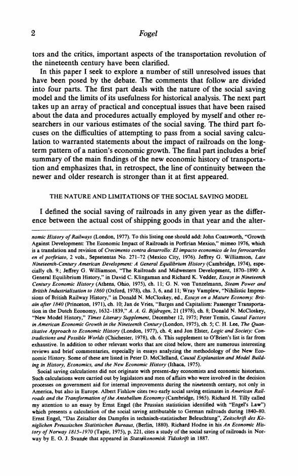
Table 2 shows that even with a quite inelastic demand curve for freight and passenger transportation (e = 0.4), calculations based on the assump- tion of zero elasticity may bias the social saving estimates upward by as much as 46 percent. If the appropriate estimate of E is as much as one, which seems likely for passenger transportation, the upward bias would range up to 143 percent. Another point worth noting about Table 2 is that the potential upward biases vary quite widely from estimate to estimate. For this reason casual comparisons of different social saving estimates may be quite misleading. Fishlow argued that he could project safely his 1859 social saving to 1890 by using the ratio of railroad receipts in the two years as a blow-up factor. As I have pointed out elsewhere, this is a frail procedure and cannot be a substitute for detailed and considered calcu- lations of the type that Fishlow constructed for the antebellum U.S., Hawke for England, Coatsworth for Mexico, and Metzer for Russia. Other, more plausible but equally frail, blow-up procedures yield projec- tions less than a third of that computed by Fishlow.'3 Table 2 suggests still another reason for caution. If the elasticities of demand for freight and passengers are 0.4 and 1.0 respectively, Fishlow's estimated social saving in 1859 is, for this reason alone, too high by 39 percent.
So it seems to me that Boyd and Walton were right in urging that we go beyond calculations based on the assumption that E = 0. It is time to move from guesses about the relevant elasticities to estimation of them. Toward that end, a number of regression estimates of demand, supply, and cost curves are presented later in this paper. Although based on the limited data available in published sources, these regressions do suggest that much progress can be made toward producing reasonably tight estimates of critical parameters, especially if the abundant data in government and private archives are used.
13 Fogel, Railroads, pp. 219-34; Robert W. Fogel, "Railroads as an Analogy to the Space Effort," Economic Journal, 76 (Mar. 1966), 16-43.
12 Fogel
TABLE 2 ESTIMATES OF THE POTENTIAL UPWARD BIAS (B) IN THE SOCIAL SAVING
ESTIMATES OF FOGEL, FISHLOW, AND HAWKE AS A FUNCTION OF e (bias in percent)
5 6 Hawke's Hawke's Passenger Passenger
Social Social Saving Saving
1 2 3 4 with an witha Fogel's Fishlow's Hawke's Fishlow's Infinite Zero
Agricultural Freight Freight Passenger Elasticity Elasticity Social Social Social Social of Demand of Demand Saving Saving Saving Saving for Comfort for Comfort
\ 1.87 3.33 2.64 2.52 2.39 4.82
0.0 0 0 0 0 0 0 0.4 15 32 24 23 21 46 0.75 28 66 49 46 43 98 1.0 39 94 69 64 60 143 1.5 62 158 113 105 97 251 2.0 87 233 164 152 139 382
Note: The entries for B are computed from equations (13) and (14) in the text. The sources of the data from which the values of 0 were calculated are: Col. 1, Fogel, Railroads, pp. 42, 47, 84-87, 110; Table 3. Cols. 2 and 4, Fishlow, American Railroads, pp. 93, 337; cols. 3, 5, and 6, Hawke, Railways, pp. 48, 88, 141, and 188. It will be noticed that holding e constant, the greater the value of 0, the larger the upward bias in the estimated social saving.
Relationship between the Social Saving and the Social Rate of Return
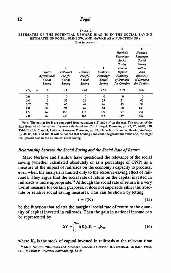
Marc Nerlove and Fishlow have questioned the relevance of the social saving (whether calculated absolutely or as a percentage of GNP) as a measure of the impact of railroads on the economy's capacity to produce, even when the analysis is limited only to the resource-saving effect of rail- roads. They argue that the social rate of return on the capital invested in railroads is more appropriate. 4 Although the social rate of return is a very useful measure for certain purposes, it does not supersede either the abso- lute or relative social saving measures. This can be shown by letting
i = f(K) (15)
be the function that relates the marginal social rate of return to the quan- tity of capital invested in railroads. Then the gain in national income can be represented by
AY f(K)dK - oKo (16)
where K0 is the stock of capital invested in railroads at the relevant time 14 Marc Nerlove, "Railroads and American Economic Growth," this JOURNAL, 26 (Mar. 1966),
111-15; Fishlow, American Railroads, pp. 52-54.

Presidential Address 13
period and i0 is the social rate of interest, which here, in order to simplify the exposition, is assumed to be independent of the investment in rail- roads.'5 Nerlove's position assumes that, when comparing any two proj- ects, if
g(Kj) > f(Ko), (17) then the g project must have made a greater contribution to national in- come than thef project. But this need not be true. Even when (17) holds, it is also possible for
f f(K)dK > J g(K)dK (18) 0 0
to hold (see Figure 2). Relationship (17) implies that if another dollar were to be invested, it would earn a higher return in g than It carries no implication as to which project contributed more to national income over the entire range of the investment in each project. To answer the question one needs relation (18).
Equation (16) is, of course, the social saving. Consequently, it is not the marginal social rate of return, which is merely a point on f(K), but the area under f(K) up to ioK0, or up to h(K) (see note 15), that measures the resource saving effected by the cumulated investment in railroads.'6
PROBLEMS OF MEASUREMENT
The preceding discussion indicated that social saving computations based on the assumption that e = 0 are inherently upward biased. Never- theless, it is possible that the execution of a computation will be based on data so defective and on statistical procedures so ill suited to the task that the inherent upward bias will be overwhelmed and the resulting computa- tion will seriously underestimate the resource saving of railroads. This is, in fact, the argument of various critics. They hold that the railroad rates employed in the several computations have been too high, that the water and wagon rates have been too low, and that major components of the so- cial saving have been omitted altogether because of such conceptional er- rors in the design of the computation as the failure to take account of economies of scale in the all-other-things sector. The balance of the sec- ond part presents evidence relevant to the assessment of these contentions.
Is If the social rate of interest was a function of the level of investment in railroads, equation (16) would become
JY | f(K)dk - KO h(K)dk,
where h(K) is the function for the social rate of interest. 16 Quite similar points were made by David, "Transportation Innovations," p. 521, and by G. R.
Hawke, Railways and Economic Growth in England and Wales 1840-1870 (Oxford, 1970), pp. 10-12.

14 Fogel
Rate of return (percent)
A C
Part A: Part B: The "f" project The "g" project
ii D
t~~~~~~~~~~ o
?_Et
0 K0 K1 Km Quantity of capital (K)
FIGURE 2 THE RELATIONSHIP BETWEEN THE SOCIAL SAVING
AND THE SOCIAL RATE OF RETURN
DISCUSSION The rate of return on railroads in 1890 is represented by the "f' project. Here the investment in
railroads (K0) has expanded to the point where the marginal social rate of return on railroad capital (i4) is equal to the social rate of return. The "g" project is new, with only Kj capital invested so far. Consequently, the marginal rate of return ij is well above io. The social saving from the investment in "g" is given by the areas CDEi0. This area is considerably smaller than the areas ABi0, which repre- sents the social saving of railroads. As the "g" project matures, the capital invested in it will increase to Km. Then the marginal rates of return on the two projects will be equal and the social saving on the "g" project will be represented by the area CFiM, which is smaller than the social saving of the "f" project.
The Representativeness of the Water Rates
Perhaps the most widespread criticism of the various social saving com- putations is that the water rates employed were unrepresentative and far too low. Peter McClelland and Harry Scheiber have focused on the water rates employed in my calculation of the interregional social saving, con- tending that my use of grain rates on the Chicago to New York route biased that estimate sharply downward. McClelland based his criticism on the fact that the New York to Chicago rate was much lower than either the Buffalo to New York rate, which he placed at 0.35 cents per ton-mile, or the St. Louis to New Orleans rate, which he placed at either 0.27 or 0.19 cents per ton-mile, depending on whether one employed the "less- than-carload" or the "bulk" rate. Scheiber's criticism was based on the av- erage rate prevailing on Ohio canals during the late antebellum years, which he put at 1.4 cents per ton-mile.'"
7 Peter McClelland, "Railroads, American Growth and the New Economic History," this JOUR- NAL, 28 (Mar. 1968), 106; Harry N. Scheiber, "On the New Economic History-and Its Limitations," Agricultural History, 41 (Oct. 1967), 387.
Presidential Address 15
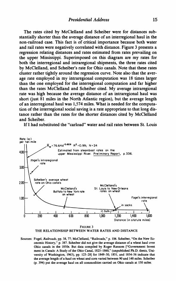
The rates cited by McClelland and Scheiber were for distances sub- stantially shorter than the average distance of an interregional haul in the non-railroad case. This fact is of critical importance because both water and rail rates were negatively correlated with distance. Figure 3 presents a regression relating distances and rates estimated from rates prevailing on the upper Mississippi. Superimposed on this diagram are my rates for both the interregional and intraregional shipments, the three rates cited by McClelland, and Scheiber's rate for Ohio canals. Note that these rates cluster rather tightly around the regression curve. Note also that the aver- age rate employed in my intraregional computation was 18 times larger than the one employed for the interregional computation and far higher than the rates McClelland and Scheiber cited. My average intraregional rate was high because the average distance of an intraregional haul was short (just 81 miles in the North Atlantic region), but the average length of an interregional haul was 1,574 miles. What is needed for the computa- tion of the interregional social saving is a rate appropriate to that long dis- tance rather than the rates for the shorter distances cited by McClelland and Scheiber.
If I had substituted the "carload" water and rail rates between St. Louis
Rote (?) per tan-mile
RW :76.64d R :0.99; Na24
l /0 Estimated from steamboat rates on the upper Mississippi River. Preliminary Report, p.336.
Fogel s introregionol rote
3.00 /
Scheibers average wheat 2.00 - \rate on Ohio canals
/ ~~~~~~~~~McClellond s McClellands St. Louis to New Orleans
Buffalo to New York rate rates on wheat ot on wheat
.00 \ / \ Fogels interregional rate
in sacks
I I I I in bulk--' I - I 0 200 400 600 800 1,000 1,200 1,400 1,600
Distance (in statute miles)
FIGURE 3 THE RELATIONSHIP BETWEEN WATER RATES AND DISTANCE
Sources: Fogel, Railroads, pp. 38, 77; McClelland, "Railroads," p. 106. Scheiber, "On the New Ec- onomic History," p. 387. Scheiber did not give the average distance of a wheat haul over Ohio canals in the 1850s. But data compiled by Roger Ransom ["Government Invest ment in Canals: A Study of the Ohio Canal, 1825-1860," (unpublished Ph.D. thesis, Uni- versity of Washington, 1963), pp. 123-281 for 1849-50, 1851, and 1854-56 indicate that the average length of a haul on wheat and corn varied between 90 and 148 miles. Scheiber (p. 394) put the average haul on all commodities carried on Ohio canals at 150 miles.

16 Fogel
and New Orleans for rates that I actually employed, the interregional so- cial saving would have changed only slightly.'8 This is because railroad rates per ton-mile over the St. Louis-to-New Orleans route were also higher than those on the Chicago-to-New York route. As I pointed out in my book, it is the difference between the water and rail rates that counts.'9
When he turned to my intraregional computation, McClelland dropped the suggestion that the Buffalo-to-New York or St. Louis-to-New Orleans rates were more appropriate than the ones I employed. Although he made no statement about the direction of bias, he contended that my intra- regional water rates were unrepresentative because they were based on re- gressions that covered only 12 of 29 commodities. Yet as I pointed out in Railroads, pp. 70-71, "These 12 commodities represented 77 percent of the tonnage shipped from counties." Moreover, "The rates on the remain- ing items were made proportional to some [comparable] commodity for which a regression equation existed. The proportions were calculated from a scattering of water tariffs that contained both a rate on the com- modity in question and on the commodity for which the regression equa- tion existed." Even if one assumes an improbably large downward bias in the rates calculated from proportions (and there is no reason to suspect a systematic bias), the small share of these commodities in the total origi- nated tonnage as well as the small share of water costs in the total of intra- regional shipping charges would make the estimate of the intraregional social saving insensitive to such errors. Thus, if there were a 50 percent downward error in these water rates, the correction would increase the first approximation of the intraregional social saving by only 3.5 per- cent-that is, it would raise the first approximation from 2.5 to 2.6 percent of GNP.
Both McClelland and Paul A. David present still another reason for be- lieving that the water rates were biased downward. They contend that government subsidies for the construction of canals and for the improve- ment of natural waterways were overlooked. However, I allowed an an- nual rental charge of $18 million for uncompensated capital costs.20 Le- bergott recognized that the calculation included such an adjustment but held that it was not large enough. To demonstrate his point he multiplied the cumulated construction costs of the New York State canals to 1882 by
18 Only the third digit is changed. The interregional social saving would have risen from 0.61 to 0.64 percent of GNP and the overall social saving on agricultural products would have been raised from 1.78 to 1.81 percent of GNP. "Less-than-carload" rates are irrelevant since virtually all inter- regional shipments went at "carload" rates.
19 The railroad rate from St. Louis to New Orleans was 0.572 cents per ton-mile. This is based on a railroad rate of 20 cents per hundred pounds and a rail distance of 699 miles. See U.S. Inland Water- ways Commission, Preliminary Report of the Inland Waterways Commission, U. S. Senate, Doc. 325, 60th Cong., 1st Sess. (1908), pp. 344-45 (hereinafter referred to. as Preliminary Report); U.S. Pay De- partment (War Department), Official Table of Distances (Washington, D.C., 1906), p. 427.
20 McClelland, "Railroads," pp. 111-13; David, "Transportation Innovation," p. 513; Fogel, Rail- roads, pp. 46-47, 87-88.

Presidential Address 17
0.06 and divided the product by the ton-miles of transportation provided by that system in 1882. The resulting figure is 0.53 cents per ton-mile, which he compared to a figure implicit in my computation of 0.07 cents per ton-mile.2' There are several difficulties with Lebergott's calculation. One is that it rests on the incorrect assumption that all capital costs of ca- nals were uncompensated.22 More important is the absence of an adjust- ment for the fact that over 90 percent of water-borne freight service in 1890 took place on the Great Lakes, the coastal routes, and the western rivers where uncompensated capital charges per ton-mile were far less than they were on such artificial waterways as the New York State canals. If all federal expenditures on rivers and harbors between 1822 and 1890 are attributed exclusively to vessels engaged in the coastal and inland trade, the annual charge for uncompensated capital employed with water- borne freight, outside of canals, is just 0.02 cents per ton-mile. Con- sequently, even if one were to accept Lebergott's figure for canals, uncom- pensated capital costs over the entire waterway system would average less than 0.04 cents per ton-mile. This figure is still too high since in the ab- sence of railroads water-borne freight service would have increased greatly, and it is likely that most of the increase would have come on the Great Lakes, the western rivers, and the coastal routes.23
21 Lebergott, "United States Transportation," p. 440. 22 In 1889 state and private canals had net earnings equal to 1.3 percent of the cost of construction
(at book value). U.S. Bureau of the Census, Eleventh Census of the United States: 1890, Report on Transportation Business in the United States, Vol. 14, Part II, pp. 475, 480 (hereinafter referred to as Census of Transportation 1890).
Discounting the stream of annual expenditures on construction and operation, as well as the an- nual net earnings of the New York canals at 6 percent, it appears that over 90 percent of the capital cost had been paid by 1882. The computation is based on data in New York State, Annual Financial Report of the Auditor of the Canal Department: 1884, "Statement of Receipts and Payments in Each Year on Account of All the State Canals." Revenues were obtained by adding "Tolls" and "Rent on Surplus Water." The annual sum of capital and operating costs was estimated by adding the follow- ing annual payments: "Canal Commissioners and Superintendent of Public Works," "Repairs of Ca- nals," "Expenses of Collectors and Inspectors," "Weighmasters," and 70 percent of "Miscellaneous Expenses." It was estimated that approximately 30 percent of "Miscellaneous Expenses" was unre- lated to the operation of the canals. This procedure of obtaining the combined capital and operating expenditures was adopted because direct information on annual capital expenditures was not avail- able before 1875, but the cumulated sum of capital expenditures for the period 1817-74 is available, as are the annual construction costs for 1875-92 (see New York State, Annual Report of the State En- gineer and Surveyor: 1893, pp. 47-57). Of course if "Miscellaneous Expenditures" had been dis- aggregated, the desired annual combined cost series would have been directly available. It was pos- sible to test the assumption that 70 percent of "Miscellaneous Expenditures" was canal costs. If the annual operating costs in the Annual Financial Report (p. 63) are subtracted from the total costs com- puted from "Statement of Receipts," one obtains a series of estimated annual construction costs. The cumulated sum of this estimated series for the period 1817-74 comes to within 1.06 percent of match- ing the cumulated sum of actual construction costs for the same period reported in the Annual Report of the State Engineer. For the period 1875-82, when both annual construction and operating costs are directly available, the indirect procedure yields annual totals that are within 4.0 percent of the actual annual totals of operating and construction costs.
23 Cumulated federal expenditures on rivers and harbors during 1822-90 were $180.4 million. Ton- miles of transportation in 1889 were 1.4 billion by canal and 48.3 billion by all other domestic con- tiguous waterways. See Appendix, Section A, for a discussion of the method of computing ton-miles

18 Fogel
The foregoing comments indicate that further research into water and rail costs in 1890 and in other years is warranted not merely because it would provide a tighter estimate of the social saving but because it would deepen our knowledge of the performance characteristics of alternative transportation systems over a wide range of technological improvements, products, geography, and other economic circumstances. Work on these issues to date should be considered only a start in the right direction.
Demonstration that the water rates employed in the social saving calcu- lation were reasonably representative of the water rates actually pre- vailing in 1890, or at the end of whatever period might be relevant, does not rule out the possibility that these rates introduced an upward bias into the social saving calculation. One must still deal with the question of what the water rates would have been in the absence of railroads. I assumed that the long-run cost curve of water transportation was either constant or, more likely, declining.24 The same assumption was made by some but not all of the others who computed a social saving. No elaborate econometric justification for the assumption of a fall in water rates with the size of ves- sels and canals seemed needed since that assumption is embedded deeply in the engineering and transportation literature of the nineteenth and twentieth centuries and buttressed by much evidence for both the United States and Europe.25 I argued that in the American case the long-run cost curve appeared to be downward sloping, so that the use of observed 1890 water rates, after including an adjustment for state subsidization of water transportation, would bias the computed social saving upward.
This proposition has been challenged by Lebergott, McClelland, David, Meghnad Desai, Donald Wellington, Cohn M. White, and G. N. von Tunzelmann.26 They have raised two principal objections to the use of ob- served water rates in 1890 or, more generally, at the end of the period un- der study. One rests on the assumption that canal transportation was in- herently monopolistic and that the competition of railroads was necessary to prevent water rates from being raised to monopolistic levels. Hence it is argued that even if the long-run cost curve were constant or declining,
of water transportation and the average water haul. Harold Barger, The Transportation Industries 1889-1946 (New York, 1951), pp. 254-55; Census of Transportation 1890, Part II, pp. xi-xiii, and passim; U.S. Bureau of the Census, Historical Statistics of the United States, Colonial Times to 1970 (Washington, D.C., 1975), p. 765 (hereinafter referred to as Historical Statistics); New York State, Committee on Canals, Report of the Committee on the New York Canals, 1899-1900, pp. 181-84 (here- inafter referred to as New York Canals); George G. Tunnell, "Statistics of Lake Commerce," U.S. House of Representatives, Doc. No. 277, 55th Cong. 2d Sess., passim.
24 By "long-run" I mean that capital is fully variable, so that the size of canal locks, prisms, and vessels on all the relevant waterways (actual or potential) could be increased as warranted by the in- creased traffic.
25 This evidence is discussed below. 26 Meghnad Desai, "Some Issues in Econometric History," Economic History Review, 2nd Ser., 21
(1968), 1-16; Donald Wellington, "The Case of the Superfluous Railroads," Economic and Business Bulletin, 22 (Fall 1969), 33-38; Colin M. White, "The Concept of the Social Saving in Theory and Practice," Economic History Review, 2nd Ser., 24 (1976), 82-100.
Presidential Address 19
monopolistic practices would have led to a rise in water rates in the ab- sence of railroads.27 The second objection is to the proposition that the long-run marginal cost curve of water transportation was downward slop- ing. A variety of arguments, mainly of an a priori nature, have been set forth to support the counter proposition that the long-run marginal cost curve was rising.
The Effect of Monopoly Pricing by Waterways
McClelland and the others who have raised the monopoly issue have not confined themselves to the question of the direction of the effect, but have also suggested that the magnitude is so large as to render the social saving computation worthless. Yet it can be shown that even if the con- jecture about the direction of the bias were correct, the magnitude would be moderate, at least in the American case. This is because canals would have provided only a relatively small fraction of the transportation service required in the absence of railroads. The point is illustrated by Table 3, which shows the approximate distribution of the payments required to move agricultural products from farms to secondary markets on the as- sumptions that E = 0 and canals charged long-run marginal costs. Suppose that in the absence of railroads, canal owners doubled the charge for us- ing canals. Then, if we continue to assume that E = 0, which is the as- sumption that maximizes the impact of the monopolistic practice, the ex- tra cost of shipping would be $39 million (see Table 3), which if added to my estimate of the social saving before adjustment for limited tech- nological adaptation would raise that estimate from 3.4 to 3.7 percent of GNP. Even if warranted, this correction is not so large that it alters the basic analysis of the resource-saving effect of railroads.28
This correction is not warranted, however, and should not be made. Contrary to the assumptions of those who raised the monopoly issue, mo-
27 Much of the discussion has failed to distinguish between the equity and efficiency effects of mo- nopoly pricing. As will be shown below, to the extent that canals used monopoly power to set rates above marginal costs, the increased revenue was mainly an income transfer.
281 In this connection it should be noted that my estimate of the effect of an extension of the canal system on the social saving (cf. Fogel, Railroads, pp. 94-98) is also robust with respect to a plausible range of error in the estimate of Construction costs. Assuming that the combined annual interest and depreciation rates were 0.07, the annual rental cost of the canal extensions would be $11.3 million. Consequently, if construction costs were twice that indicated by the regression, my estimate of the ag- ricultural social saving would rise from 1.8 to 1.9 percent of GNP.
The same point holds with respect to the argument that some of the rivers designated as navigable by the Army Engineers were too shallow to handle the volume of traffic that would have been di- verted to these waterways in the absence of railroads. Such a contingency could have been handled by canalizing these rivers or building parallel canals along the necessary portions of the rivers in ques- tion. If we suppose that the increased traffic would have required parallel canals along 5,000 miles of such rivers (this is considerably greater than the mileage of the navigable rivers thus far contested), the additional construction costs would once again raise the social saving by just one tenth of 1 per- cent of GNP. Cf. Gilbert Fite, review in Agricultural History, 40 (Apr. 1966), 147-49; John A. Shaw, "Railroads, Irrigation, and Economic Growth: The San Joaquin Valley of California," Explorations in Economic History, 24 (Winter 1973), 211-27.

20 Fogel
TABLE 3 APPROXIMATE COST OF MOVING AGRICULTURAL PRODUCTS FROM THE
FARMS TO THE SECONDARY MARKETS OF THE U.S. IN THE NON-RAILROAD CASE, ASSUMING THAT CANALS CHARGED LONG-RUN MARGINAL COST, THAT e= 0, AND ALLOWING
NO EXTENSION OF CANALS OR IMPROVEMENT OF COMMON ROADS
3 4 Cost of Percentage
1 Service Distribution Ton-miles 2 (million of Total of Service Rate dollars) Cost among
Category of Service (millions) (dollars) (Col. 1 x Col. 2) Services
1. Wagons 3,107 0.165 513 65 2. Canals 3,505 0.011 39 5 3. Other waterways 26,805 0.0050 134 17 4. Waterway-associated
services (insurance, transshipping, storage) 107 13
5. Totals 33,417 793 100
Notes: Column 1, line 1: Approximately 36.8 million tons shipped an average of 62.7 miles to wa- terways. An additional 23.5 million tons shipped an average of about 28 miles from farms to local purchasers. An additional 142 million ton-miles were allowed for the wagon portion of shipments go- ing by waterways to secondary markets. Fogel, Railroads, pp. 42, 46, 76, 86, 87; cf. Winifred Rothen- berg, "The Marketing Perimeters of Massachusetts Farmers, 1750-1855" (mimeo, Brandeis Univer- sity, 1978). Line 2: Approximately 10 percent of intraregional railroad shipments sent an average of 150 miles; approximately 75 percent of interregional shipments sent an average of 250 miles. Fogel, Railroads, 42, 84-87. Line 3: Approximately 90 percent of intraregional rail shipments sent an aver- age of 150 miles; approximately 75 percent of interregional shipments sent an average of 1324 miles; approximately 25 percent of interregional shipments sent an average of 1574 miles; ibid.
Column 2, line 1: Fogel, Railroads, pp. 84, 86. Lines 2 and 3: Average interregional rate (Fogel, Railroads, p. 42), adjusted to consider distances indicated in notes to column 1, lines 2 and 3, and weighted by corresponding ton-miles. U.S. Inland Waterways Commission Preliminary Report, U.S. Sentate, Doc. 325, 60th Cong. Ist Sess., 1908, p. 336. Allowance for neglected capital costs (Fogel, Railroads, p. 47) distributed according to ton-miles.
Column 3, line 4. Fogel, Railroads, pp. 47, 92.
nopoly in water transportation implies that there was an upward rather than a downward bias in the estimated social saving. Two points are in- volved here: one historical, the other analytical. The historical issue bears on the way in which the monopoly would have been exercised. Lebergott, McClelland, and the others assumed that monopoly power would have been exercised to raise water rates. This is quite a reasonable assumption for the English case where most canals were privately owned and where there is considerable evidence that canal tolls charged before the coming of the railroad were in excess of marginal costs. For this reason Hawke, after an examination of the pre-railroad pricing policy of canals, assumed that monopoly power was used to inflate tolls on average by 150 percent. In addition to the toll, there was a payment to the owners of the boats that carried the freight. Both in England and the United States the boat own-
Presidential Address 21
ers were numerous and operated competitively.29 Taking both the toll and the boat charge into account, Hawke estimated that in the absence of rail- roads the canal shipping rate would have increased by approximately one third.30
The American case is entirely different. More than 80 percent of the tonnage shipped via canal in 1890 was borne on canals owned not by pri- vate firms but by state governments or the federal government.3" These governments used their monopoly power to lower tolls below marginal costs rather than to raise them above marginal costs.32 The policy of sub- sidizing canal transportation was not due to the competitive pressure of the railroads but to political pressure put on government officials by the users of transportation. Roger Ransom, who studied the Ohio Canal, esti- mated that even in the 1830s and 1840s, before railroad competition be- came significant in that state, tolls were not set high enough to cover long- run marginal costs." In the American case, parties on all sides of the transportation debates of the nineteenth century agreed that it was the competitive pressure of waterways that kept railroad rates low, rather than the competitive pressure of railroads that kept waterway rates low. "Railroad companies," said Albert Fink, Commissioner of the Trunkline Executive Committee, "fully recognize the potent influence of water com- petition and are not afraid of it, but on the contrary, they have met it and must meet it wherever they find it, without complaint and as one of the inevitable conditions under which they have to struggle for existence."34 Since there is no historical basis for the proposition that U.S. canals, in the absence of railroads, would have pushed tolls above marginal costs,
29 New York State, Annual Financial Report of the Comptroller, Relating to Canals: 1884 Assembly, Vol. 1, No. 4, p. 17, commented on the devastating effects of the business cycle recession that began in 1882 on canal operators. Their difficulties, the report said, were due to their failure to combine and act monopolisti Uy:
On the 1st of January, 1883, there were 4,749 boats of all classes registered as navigating the State canals.... If the canals with their equipments were owned by a corporation, or even if the equipments only were under one management, they would represent a single harmonious system competing with the railways in the transportation of freight. As they are now operated and man- aged, the equipments are furnished by almost as many individual owners as there are boats, and representing as many conflicting interests. These owners are without organization.... 30 Hawke, Railways, pp. 80-86. 3' Census of Transportation 1890, Part II, pp. 469-79; cf. Preliminary Report (1908), pp. 188-209. 32 As pointed out in footnote 22, state and private canals reported combined net earnings in 1889
that amounted to just 1.3 percent of their cost of construction. Census of Transportation 1890, Part II, pp. 475, 480. See the section, The Representativeness of the Water Rates for a discussion of my upward adjustment in water rates to compensate for the subsidy of the capital employed in water transporta- tion.
33 Roger L. Ransom, "Government Investment in Canals: A Study of the Ohio Canal, 1825-1860," unpublished Ph.D. dissertation, University of Washington, 1963, pp. 135-36. The tolls represent the receipts of the canal but not the entire benefit of the canal. When external benefits were added to the canal receipts, Ransom obtained a social rate of return for the 1840s that exceeds the market rate of return.
I Cited in Lewis M. Haupt, "Canals and their Economic Relation to Transportation," Papers of the American Economic Association, Series I, Vol. 5, No. 3 (1890), p. 67.

22 Fogel
the question of whether an upward adjustment of the observed rates should be made on this account need not be pursued further.
The issue does have to be pursued in the English case, where Hawke es- timated that canal shipping rates, in the absence of railroad competition, would have exceeded marginal cost by about one third. Contrary to some current arguments, however, the appropriate adjustment for this monop- oly power will reduce rather than increase Hawke's estimated social sav- ing. If this result seems paradoxical, it is because so much attention has been directed to demonstrating that the counterfactual water rates would have been higher than observed water rates. Consequently, another and quantitatively far larger effect going in the opposite direction has been overlooked. That is the bias due to the assumption that e = 0. If canal owners were, in the absence of railroads, monopolists maximizing profits by setting prices in such a way as to equate marginal revenues and mar- ginal costs, then they must have been operating in the elastic portions of their demand curves. Indeed, we can infer the relevant elasticity of de- mand by inserting Hawke's estimates of the ratio of canal rates to mar- ginal costs into the well-known equation relating price, marginal revenue, and the elasticity of demand, which may be written as:
I = p I .(19)
fR_ Since profit is maximized when marginal cost equals marginal revenue, (19) becomes
e= PI * (20)
It follows from equation (20) that if the price of canal transportation ex- ceeded marginal cost by about a third (P/MC ~ 1.32), then the elasticity of the demand for canal transportation was in the neighborhood of 3. Even if we take the case of the Leeds and Liverpool Canal, where the dis- crepancy between price and marginal cost was substantially greater than Hawke (p. 84) thought was typical, the implied value of e is 1.1. In either case, it follows from Table 2 that Hawke's assumption that e = 0 in- troduced a substantial upward bias into his estimate of the freight social saving, a bias that is much larger than the downward bias due to his ne- glect of the misallocation of resources associated with monopoly pricing.
Both biases are measured and shown in Figure 4 and Table 4. In Part A of Figure 4, the demand curve XX has an elasticity of 1.1. The social sav- ing of ?26.6 million, as calculated by Hawke, is represented by the area (Pw - Pr) Qr. But if e = 1.1, the quantity of transportation demanded at the rate of PW is Qw, and that is just one third of the ton-miles provided in the railroad case. Consequently, the social saving is reduced to ?15.0 mil- lion, which is represented by the area PwCEPr. It follows that the upward

Presidential Address 23
x x
PAR Ae=1.PARTB
FIUR 4
C ? ~~AD TH CS UPTO DHT
variable an ae dl here.
bility of m p p b ll i
DIGAIHWN H PADADDWWR BIAESIN HAK'RIH
Notet ofthis darmisholdocationsideredsn onunctio attibthable 4toih ie the vales of thea
bilihtyof monpol ps ng by ceandL amouns i ist repe-
PwThti Eersne byteae ACadaout ojs EO4ml
lion. The area (Pw'-Pw) * Qw', which comes to ?2.5 milon, is not a reduc- tion in real income but, as Hawke pointed out, an income transfer. Thus the downward bias in Hawke's social saving calculation due to misalloca- tions attributable to canal monopoly pricing is hardly 3 percent of the up- ward bias due to the assumption that e = 0.
The last finding does not rest on the assumption that the elasticity of demand for transporting was greater than one. Part B of Figure 4 and col- umn 2 of Table 4 give simiar results for the case in which e = 0.5. Even with this rather inelastic curve, the ratio ofwthe 4,which gv the valueseupward bias is just 4 percent, and Hawke's net overestimate of the "true" social saving is 30 percent.
The Shape of the Long-Run Marginal Cost Curves of Waterways
Analysis of the long-run marginal cost curves of waterways did not be- gin with the debate over the social saving of railroads. It originated with

24 Fogel
TABLE 4 THE CALCULATION OF THE BIASES IN HAWKE'S FREIGHT SOCIAL SAVING
ESTIMATE DUE TO THE MONOPOLY PRICING BY CANALS AND THE ASSUMPTION THAT E = 0
Values of Variables and Areas When Variables and Areas Shown in Figure4 0=l.l E=O.5
1. Pr 1.23 d 1.23d 2. P, 3.24d 3.24d 3. Pw 3.93d 3.93d 4. Qr(in ton-miles) 3,175 X 106 3,175 x 106 5. Qw (in ton-miles) 1,060 x 106 1,956 x 106 6. Qw' (in ton-miles) 857 x 106 1,776 x 106 7. Pr-Qr ?16.27 X 10⁶ ?16.27 X 10⁶ 8. Pw-Qr ?42.86 X 10⁶ ?42.86 X 10⁶ 9. PW- ?14.31 X10⁶ ?26.41 x 10⁶
10. PW' QW' ?14.03 X 10⁶ ?29.08 x 10⁶ 11. (Pw-Pr)Qr ?26.59 x 10⁶ ?26.59 x 10⁶ 12. PwCEPr ?15.03 X 10⁶ ?20.27 X 10⁶ 13. CDE ?l1.56 x 106 ?6.32 x 10⁶ 14. ABC ?0.36 x 10⁶ ?0.24 x 10⁶ 15. (PW'-PW)Qw ?2.46 x 10⁶ ?5.11 x 10⁶
Sources and Notes. Line 1: P. exceeds the figure of 1.21d given by Hawke for 1865 (Hawke, p. 62) because of the addition of 55 X 106 ton-miles for livestock not included in Hawke's figure of 3,119.6 X 106 ton-miles and the addition of ?0.5 X 10⁶ for livestock (Hawke, p. 141) to the figure for railroad revenues that Hawke gives for 1865 on p. 88. Line 2: Computed by multiplying 1.23d by Pw Qr + Pr-Qr. Line 3: Computed by multiplying 1.23d by the sum of Pw-Q, and Hawke's estimate of the dif- ference between the saving of charges and the social saving for 1865 (p. 89) and then dividing by Pr-Qr [1.23(42.9 + 9.1) + 16.27 = 3.931]. Line 4: Hawke's figure of 3,120 x 106 (p. 62) plus an allow- ance of 55 X 106 ton-miles for livestock. This allowance was computed from the data in Hawke, pp. 140 41, on the assumption that the average weights of cattle, swine, and sheep were 1,000 lbs., 200 lbs., and 150 lbs., respectively. Hawke's figure of 309 x 106 livestock miles was inflated by the ratio of total livestock receipts to the livestock receipts covered by the ten roads in his Table V.03. Lines 5 and
'3.24
6: Computed from Q = DP-'. Line 12: Computed from DJ P` dp. Line 13: CDE = (Pw - Pr)-Qr 1.23
t3,93 - PwCEPr. Line 14: Computed from DJ P-dp less (Pw' - Pw)Qw.
3.24
the engineers who had charge of building canals or boats, and with nine- teenth-century transportation economists. The results of their investiga- tions led repeatedly to the conclusion that the unit cost of water transpor- tation decreased as boat size, tonnage carried, and distance increased. The finding soon gained the status of a self-evident proposition and is now deeply embedded in the literature of transportation engineering and eco- nomics. "In the case of waterways," wrote Kirkaldy and Evans, authors of a British textbook on transportation economics of World War I vintage, "the extra wear and tear arising from increased traffic is practically negli- gible; and the actual working experience of some of the canal companies, such as the Manchester Ship Canal, proves that this is so; that a very sub- stantial increase of traffic can be accommodated on a waterway without anything like an equivalent increase in the cost of maintenance." Otto

Presidential Address 25
Franzius, author of a leading treatise on waterway engineering, presented evidence drawn from the experience of German inland waterways. He re- ported that with a 58 percent increase in the carrying capacity of boats, construction costs per gross ton declined by 9 percent and the ship main- tenance and crew costs per delivered ton declined between 2 and 16 per- cent. Engineers consulted by the U.S. Senate Select Committee on Trans- portation Routes to the Seaboard (Windom Committee) in the early 1870s concluded that "the enlargement of the New York canals so as to pass boats of 600 to 1,000 tons, will reduce the cost of transportation on that part of the line 50 per cent."35
David questioned my assumption that the long-run marginal cost curve of waterways was downward sloping because "only one page is devoted to supporting this assertion," and he found it to be "not a very satisfactory page."36 Even though it is now obvious that my discussion was too brief, the fact remains that the issues that most concerned David, such as the adequacy of the water supply, were investigated in detail by engineers ap- pointed by various federal, state, and private agencies. Their findings, which are set forth in published documents as well as in secondary sources, were not only that the water supply was plentiful but that the en- larged canals would have reduced per ton-mile costs.37
Desai and von Tunzelmann argued that because water transportation was a shrinking industry only the most efficient carriers would have sur- vived. From this a priori statement they drew two conclusions: one is that the long-run supply curve was upward sloping; the other is that use of the waterway rates of 1890 imparted a downward bias to the social saving cal- culAtion.38 Suppose it were true that water transportation was a shrinking industry. In order to proceed from this proposition to the conclusion that the long-run cost curve is upward sloping, it is necessary to consider the characteristics of both the enterprises that went out of business and those that survived. The boatmen who continued to operate owned larger ves-
1s Adam W. Kirkaldy and Alfred Dudley Evans, The History and Economics of Transport (London, 1915), p. 221; Otto Franzius, Waterway Engineering (Cambridge, 1936), pp. 433-35; U.S. Senate, Se- lect Committee on Transportation Routes to the Seaboard, Report No. 307, 43d Cong., 1st Sess., Vol. 1, p. 247. Cf. also J. Stephen Jeans, Waterways and Water Transport (London, 1890), ch. 27; Edwin F. Johnson, The Navigation of the Lakes and Navigable Communications Therefrom to the Seaboard, and to the Mississippi River (Hartford, 1966); John R. Meyer, Merton J. Peck, John Stenason, Charles Zwick, The Economics of Competition in the Transportation Industries (Cambridge, Mass., 1959), pp. 111-13; J.E. Palmer, British Canals: Problems and Possibilities (London, 1910), ch. 3. See also the sources cited in William Pierson Judson, History of the Various Projects, Reports, Discussions, and Es- timates for Reaching the Great Lakes from Tide- Water, 1768-1901, Oswego Historical Society, Pub. No. 2. (Oswego, N.Y., 1901). The Index to the Reports of the Chief of Engineers, U.S. Army, 1866- 1912, U.S. House of Representatives, Doc. No. 740, 63d Cong., 2d Sess., 2 vols., lists many reports investigating the relationship between waterway costs and vessel size, prism size, distance, and so forth.
36 David, "Transportation Innovation," p. 511. 37 See the sources cited in footnote 35. 38 Desai, "Some Issues," p. 10; von Tunzelmann, Steam Power, pp. 39-41.

26 Fogel
sels than those who retired, and the canals that survived could accommo- date larger vessels than those that were abandoned.39 The fact that it was the larger boats and canals that tended to survive and the smaller ones that tended to fail is primafacie evidence of economies of scale and hence quite in keeping with the engineers and transportation economists who held that the long-run cost curve was downward sloping. Moreover, al- though it is true that the traffic on most canals was shrinking, the traffic on the waterway system was not. The traffic on the Great Lakes, the coastal routes, and the Mississippi system was growing at a fairly high rate, al- though not as rapidly as railroad freight. The registered tonnage of sailing and steam vessels on the Great Lakes increased at an annual rate of 3.3 percent between 1868 and 1890. Consequently, waterways still accounted for over a third of all non-wagon freight ton-miles in 1889.4 Nor should one exaggerate the decline of business on the canals. On the New York State canals traffic in 1890 was virtually at the average level of the pre- vious two decades, and well above the pre-Civil War average.4"
It is possible to test the judgment of the engineers and transportation economists by estimating waterway cost functions. Equation (21), which relates the construction cost of a canal to the cross section of its prism (Xp), the length of the canal (X,), and its total blockage (Xr), is estimated from data compiled by H. Jerome Cranmer. His data set covers 44 canals that accounted for 79 percent of total canal investment prior to 1860.42
Cc = -0.5883 + 0.5103Xp + 0.6851X, + 0.0550Xr (21) (1.0894) (0.2069) (0.1308) (0.1139)
R2 = 0.82; N = 44
Since this equation is log-linear, the coefficients are elasticities, and each coefficient, minus 1, yields the relevant elasticity of marginal cost. It is evi- dent that the marginal cost of canal construction declined with increases in all of the variables, although the effect on cost of a canal's rise and fall (Xr) was slight.
Equation (22) relates the annual operating costs of canals to capacity (as measured by prism size) and total freight carried (Xf). It is estimated for 1889 from a cross-sectional regression on 13 canals.43
CO = 5.6857 - 1.0905XP + 0.9230Xf (22) (2.4032) (0.5385) (0.0996)
R2=0.90;N= 13
39 New York Canals, p. 171; U.S. Bureau of Statistics (Treasury Dept.), "The Grain Trade of the United States," Monthly Summary of Commerce and Finance, No. 7, Series 1899-1900 (Jan. 1900), p. 1972; Preliminary Report, pp. 193-209; H. Jerome Cranmer, "Canal Investment, 1815-1860," in Con- ference on Research in Income and Wealth, Trends in the American Economy in the Nineteenth Cen- tury, Vol. 24 of Studies in Income and Wealth (Princeton, 1960), p. 564; Census of Transportation 1890, Part II, pp. 474-77; Tunnell, "Statistics," pp. 3, 4, 26.
4 Barger, The Transportation Industries, p. 184, and the Appendix, Section A, below. 4' New York Canals, pp. 181-83. 42 Cranmer, "Canal Investment," pp. 547-64. Figures in parentheses are standard errors. 43 The data for this regression are from Census of Transportation 1890, Part II, pp. 475-83, 484.

Presidential Address 27
It is evident from equation (22) that the marginal cost of canal opera- tions with respect to total tonnage carried is declining. Moreover, since this equation was estimated over canals with prisms of varying sizes, it permits one to determine how canal operating costs vary when the size (Xp) of the canal itself may vary. If canal size (Xp) is held constant, and given the range within which these canals were operating, which was far below capacity, a 100 percent increase in the tonnage carried would have increased operating costs by just 90 percent. Thus if canals could only ex- pand traffic within the limits of the existing system, they would have expe- rienced moderately declining marginal costs up to the bottleneck point.
If an increase in freight brought canals beyond the bottleneck point, then it would have paid to enlarge the canals to accommodate the in- creased traffic. Suppose, for example, that canal traffic would have in- creased threefold in the absence of railroads. This would have pushed most canals past their bottleneck points, thus requiing enlargements. If canals responded by doubling capacity, then it follows from equation (22) that total operating costs would have increased by 29 percent (2-1Im-530923o= 1.29). Operating costs per ton, however, would have de- clined by 57 percent [1 - (1.29 + 3) = 0.57]. The construction costs of the enlarged canals would have been greater than the costs of those they re- placed. It follows from equation (21) that doubling the capacity (Xp) of the canals would have made the new canals 42 percent more expensive than the old ones (20.51 = 1.42). Assuming unchanged interest and depreci- ation schedules, the annual capital charge would have risen by 42 percent, but capital charges per ton would have declined by 53 percent [1 - (1.42 +
3) = 0.53]. Since capital charges were on the order of 80 percent of the an- nual long-run cost of canals, overall canal charges per ton would have de- clined by a little over 53 percent."
There is still the question of the long-run curve of the vessels that ac- counted for about half the cost of shipping by canal and virtually all of the cost of shipping on the Great Lakes, the coastal routes, and the rivers. Unfortunately, the data needed to run regressions that relate the marginal cost of boats on these routes to tonnage are not readily available. This task should be undertaken in the future, but not because the tenets of the engineers are really in doubt. That both construction costs and manning costs per gross ton fell with the volume of the ship is quite well estab- lished. Such regressions would be useful because they would give a much more precise picture of the nature of specific water alternatives and would permit a reduction of the upward bias in current social saving estimates.
McClelland presented a table and chart showing that freight rates for flour carried on the Erie Canal varied sharply during the navigation sea- son. These data reveal that in each of the five years from 1859 through
" Assuming that the depreciation and interest rates summed to 0.07, the annual rental value on the construction costs (book value) of state and private canals in operation in 1889 is $10.5 million. The operating expenses of the same canals in 1889 were $2.1 million. Census of Transportation 1890, Part II, pp. 475, 480.

28 Fogel
1863, rates reached a peak in November, during which time they were 37 to 138 percent higher than the rates of the preharvest months of May and June. McClelland contends that these data undermine Fishlow's assume tion of constant or decli nig long-run marginal cost and invalidate his use of 1859 waterway rates as measures of marginal cost.45 But monthly data have little bearing on the question of long-run costs. With the stock of boats virtually fixed over any given navigation season, all rates were quasi-rents that may have been above or below long-run marginal costs. Normally the rates would have been below long-run marginal cost in the preharvest months and above long-run marginal cost during the months immediately following the harvest. If the revenue of vessels over the entire season equaled their annual long-run marginal cost, the industry would be in long-run equilibrium, even though rates in any given month were ei- ther above or below the long-run equilibrium rate. The response to long- run disequilibrium rates would have been spread out over a number of years by boat owners who would either have added to the stock of vessels or have failed to replace vessels that were retired.
McClelland's point is useful as a caution against inadvertently choosing a rate, such as the May or June rate, that was far below long-run marginal costs. But his criticism of Fishlow was misdirected, since 1859 and 1860 were fairly normal years and Fishlow used annual average rates and not the rates of a particular month. McClelland was also in error in suggesting that the transitory rise in average annual rates during the Civil War surge of traffic implied that the Erie Canal was operating in the zone of increas- ing marginal costs. Equation (23) relates the real annual operating costs of the New York canals over the years 1853-1880 to the average length of a haul (Xd), total tons shipped (Xf), and a dummy variable representing the Civil War years (Xo,).'
CO = 13.4337 + 0.422OXf- 1.2133Xd - 0.1449X, (23) (3.8241) (0.2621) (0.6547) (0.1536)
R = 0.26; N = 28; D.W. = 1.34
Since the coefficient on Xf is less than 1, it is quite clear that on the New York State canals, as on other canals, marginal cost declined as the ton- nage shipped increased. Moreover, since the coefficient on distance (Xd) is negative, and since the effect of the Civil War was to increase the propor- tion of long hauls in grain shipments, this factor would have led to a de- cline in marginal costs.4' That the dummy variable (X,,) for the Civil War
" McClelland, "Railroads," pp. 115-20. 4 The data for this regression are from New York State, Annual Financial Report of the Comptroller
Relating to Canals: 1884, p. 63; New York Canals, pp. 156-57, 181. C. was deflated by the Warren- Pearson price index.
4 Since operating costs were less than 20 percent of the annual long-run cost of the New York ca- nals, one cannot rule out a priori the negative coefficient on Xd. On the other hand, it is possible that the mix of commodities transported was changing over time in such a way that an appropriate mea- sure of this mix would be positively correlated with distance and negatively correlated with costs (or
Presidential Address 29
years is negative (although not statistically significant) after account is taken of tonnage and distance, suggests the existence of other war-related factors that served to reduce canal operating costs. Consequently, the Civil War experience of the New York canals tends to confirm rather than refute the proposition that the long-run marginal cost of canal shipping declined as the tonnage transported increased. The transitory rise in over- all rates (payments to boats plus tolls) between 1860 and 1863 thus ap- pears to have been due to a lagged response in the supply of boats and ei- ther deliberate setting of tolls above costs by the canal authorities (perhaps prompted by wartime exigencies) or errors on their part in antic- ipating the prices of their inputs.48
The Elasticity of Substitution and the Cross Elasticity of Demand
In Railroads and American Economic Growth, I pointed out that argu- ments which inferred the indispensability of railroads from their victory over waterways in the competition for the carriage of the nation's freight involved the implicit assumption that the elasticity of substitution be- tween these two forms of transportation was quite low. But suppose the elasticity of substitution was moderately high. Then the shift to railroads could have been induced by a relatively small cost differential between railroads and waterways, and the resource saving attributable to railroads would be relatively low. I argued that the issue could only be settled by measuring the cost advantage of railroads, and so proceeded to compute the social saving on the transportation of agricultural products.
A number of investigators have taken up the point on the elasticity of substitution and pushed it in a direction that is both novel and surprising.
vice versa), when total tonnage shipped is held constant. Then the negative coefficient of Xd would be due to the omission of a mix variable. Tests of such an hypothesis were unsuccessful because of diffi- culties in constructing an appropriate index of commodity mix from published data, although all the regressions attempted yielded a negative coefficient on the Civil War dummy. An alternative ap- proach is to regress total costs on the logarithm of ton-miles and a Civil War dummy; this is equiva- lent to imposing the constraint that the coefficients on tons and on distance are the same. The results of this regression were as follows:
CO 12.7608 + 0.04998 Xgm-0.3404 X, (4.035) (0.1967) (0.1259)
R2 =0.17; N = 28; DW 1.17
A likelihood ratio test rejects the restriction at the 5 percent level but not the 2.5 percent level. Note that the Civil War dummy is still negative and is now statistically significant. The various regressions suggest the need for further research into canal cost functions, and especially into the effect of the shifting commodity mix on total costs. Pursuit of this line of analysis, however, requires the retrieval of unpublished data.
48 The same basic point was made by Fishlow who noted that "McClelland's ... own data show that a doubling of canal traffic between 1859 and 1863 left canal freight rates virtually unchanged! Over the interim, they had temporarily risen owing to adjustment problems, to be sure, but that is totally irrelevant to the long-run question under consideration." See Albert Fishlow, "Internal Trans- portation," in Lance Davis et al., American Economic Growth: An Economist's History of the United States (New York, 1972), p. 516. It might be added that it is unlikely that the supply of canal boats had reached long-term equilibrium by 1863.

30 Fogel
The first to do so was Lebergott, who argued that since canals and railways were sellers of equivalent transportation services and since they competed vigorously with each other, in long-term equilibrium they had to charge identical prices; otherwise the more expensive service would have been driven out. He concluded, therefore, that a positive social sav- ing was merely "a measure of estimating error."49
The difficulty with this argument becomes apparent when it is extended to wagons. Wagons and railroads co-existed, offered alternative means of performing the same service, and competed vigorously with each other. Hence wagon and railroad costs must have been equal; otherwise the more expensive form of transportation would have been driven out. Since we know that wagon rates, in the American case, were an average of 10 to 20 times higher than railroad rates, this argument obviously is fallacious. The point, of course, is that wagons, railroads, and waterways co-existed even though they charged different rates because they were not perfect substitutes for each other. All three co-existed because each had an ad- vantage over the others in the functions in which it specialized. Down to the end of the nineteenth century wagons, with average hauls of less than 20 miles, dominated short-haul transportation and could, despite their high average rate, usually deliver goods over very short distances more cheaply than could either waterways or railroads. American railroads, with average hauls in 1890 of about 250 miles, had their greatest advan- tage in short-to-medium distances. The advantage of waterways, with av- erage hauls in 1889 of about 650 miles, was in medium-to-long distances, especially with bulky, low-value items such as grain, lumber, coal, and ore.50
Given the specialized characteristics of each medium and the variety of requirements of shippers, one would hardly expect the elasticity of sub- stitution between the waterway and railroad systems to be infinite. Hawke recognized this difficulty and sought to refine the argument by limiting its application only to waterways and railways that directly confronted each other (as in the competition of the railroad trunk lines with the vessels of the Great Lakes and Erie Canal) and that carried "the same freight ... between the same points." In such cases, he said, the "difference in costs and charges," including "hidden costs," must "be precisely zero." Turning to the case of wagons, Hawke said that the situation was quite different since wagons were "not required to perform the same services as
49 Lebergott, "United States Transportation," p. 439. Cf. David, "Transportation Innovation," p. 513; McClelland, "Railroads," p. 114; Peter D. McClelland, "Social Rates of Return on American Railroads in the Nineteenth Century," Economic History Review, 2d Ser., 22 (Aug. 1972), 477-78; White, "The Concept," p. 85; Colin M. White, "Railroads and Rigor," Journal of European Economic History, 4 (Spring 1975), 194. The preceding writers held that I failed to recognize that railroads and waterways provided a homogeneous product. Desai ("Some Issues," p. 10), on the other hand, held that I assumed perfect substitutability. He contended that it was the heterogeneity of railroad and wa- terway services that undermined my analysis.
I The average haul of railroads in 1899, was 247 miles (Historical Statistics, p. 733). The method of estimating the average distance of a water haul in 1889 is given in the Appendix, Section A.
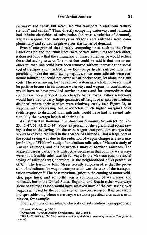
Presidential Address 31
railways" and canals but were used "for transport to and from railway stations" and canals.5' Thus, directly competing waterways and railroads had infinite elasticities of substitution (or cross elasticities of demand), whereas wagons and waterways or wagons and railroads were com- plementary and so had negative cross elasticities of demand.
Even if one granted that directly competing lines, such as the Great Lakes or Erie and the trunk lines, were perfect substitutes for each other, it does not follow that the elimination of measurement error would reduce the social saving to zero. The most that could be said is that one or an- other railroad line could have been removed without increasing the social cost of transportation. Indeed, if we focus on particular railroad lines, it is possible to make the social saving negative, since some railroads were eco- nomic failures that could not cover out-of-pocket costs, let alone long-run costs. The social saving for the railroad system as a whole, however, must be positive because in its absence waterways and wagons, in combination, would have to have provided service in areas and for commodities that could have been serviced more cheaply by railroads. Either waterways would have had to carry large quantities of freight over short-to-medium distances where their services were relatively costly (see Figure 3), or wagons, with decreasing but nevertheless much higher marginal costs (with respect to distance) than railroads, would have had to extend sub- stantially the average length of their hauls.
As I stressed in Railroads and American Economic Growth (cf. pp. 23- 25, 46-47, 51, 73, 212-14), about 85 percent of the agricultural social sav- ing is due to the savings on the extra wagon transportation charges that would have been required in the absence of railroads. That a large part of the social saving was due to the reduction of wagon charges is also a ma- jor finding of Fishlow's study of antebellum railroads, of Metzer's study of Russian railroads, and of Coatsworth's study of Mexican railroads. The Mexican case is particularly instructive because in that country waterways were not a feasible substitute for railways. In the Mexican case, the social saving of railroads was, therefore, in the neighborhood of 30 percent of GNP.52 The lesson, as John Meyer recently emphasized, is that the provi- sion of substitutes for wagon transportation was the crux of the transpor- tation revolution." The best substitute (prior to the coming of motor vehi- cles, pipe lines, and so forth) was a combination of waterways and railroads, but in the United States, England, and Russia either waterways alone or railroads alone would have achieved most of the cost saving over wagons achieved by the combination of low-cost services. Railroads were indispensable only where waterways were not a practical alternative, as in Mexico, for example.
The hypothesis of an infinite elasticity of substitution is inappropriate 5' Hawke, Railways, pp. 20-21. 52 Coatsworth, "Growth Against Development," chs. 3 and 4. 51 See his "Review of The New Economic History of Railways," Journal of Business History (forth-
coming).

32 Fogel
even when applied to such directly competing transportation modes as the Great Lakes and the trunk-line railroads. The ratio of railroad to water- way rates for wheat and other grains shipped interregionally fluctuated sharply from year to year, partly because of the intense rate wars that pe- riodically engulfed the trunk lines. If the elasticity of substitution was in- finite, these sharp fluctuations in relative rates should have led to com- plete shifts of the grain traffic from waterways to railroads and back again, as the ratio of rates swung in favor of one or the other transporta- tion mode. Although there was a certain amount of shifting in traffic with shifts in relative rates, examination of the data reveals that these shifts were too moderate to sustain the hypothesis of an infinite or nearly in- finite elasticity of substitution. Between 1878 and 1879, for example, the ratio of rail to water rates for wheat over the Chicago to Buffalo route fell by 49 percent and the ratio of the quantities of grain carried by water to those carried by rail fell by 50 percent, which suggests an elasticity of sub- stitution of about I. Similarly, between 1881 and 1882 the ratio of rail to water rates rose by 16 percent and the ratio of water to rail quantities rose by 22 percent, which suggests a substitution elasticity of 1.4.*54
A more reliable measure of the degree of substitutability between the Great Lakes and the railroads may be obtained by using regression analy- sis to estimate the cross elasticity of the demand for waterway transporta- tion with respect to the price of railroad transportation. Equations (24) and (25) represent the demand and supply equations for grain transporta- tion between Chicago and Buffalo, estimated by two-stage least squares from data covering the years from 1868 through 1898.55
g = 4.725 + 0.7383M + 0.9484lr -0.5514A (24) (2.76) (0.2181) (0.3024) (0.2938)
2= 0.47; N = 31; D.W. = 1.27
Qg = 1.562 + 1.7972 El, + 0.8234N + 0.7654Rib + 0.66791A (25) (7.90) (0.7245) (0.4979) (0.7874) (0.2228)
2= 0.84: N = 31; D.W. = 1.63
54 New York Canals, pp. 190, 208. Cf. footnote 55. 55 Data for these regressions were derived as follows: Rw for 1868-95, from Tunnell, "Statistics of
Lake Commerce," p. 29; Rw for 1896-98, from New York Canals, p. 190, col. 4; all values were de- flated by the Warren-Pearson price index. M, from Historical Statistics, p. 512 (converted to tons). Rr, from New York Canals, p. 190, col. I minus col. 5. The years 1868 through 1878 were years in which a premium existed on greenbacks, but the values of R. in Tunnell were given in gold. To obtain a con- sistent currency series, the rates for these years were multiplied by an implicit deflator (A/B, where A is the currency values of lake freight rates from Tunnell, p. 29; and B is the undefeated lake freight rate from New York Canals, p. 109, col. 4). The entire series was then deflated by the Warren-Pearson price index. Q. is from U.S. Bureau of Statistics, "The Grain Trade," pp. 1964-65 (converted to tons). N is calculated from the number of days between the opening of the lake at Buffalo and the closing of the Welland Canal. For the years in which the closing date of the Welland Canal was missing, the average difference between the closing dates of the Welland Canal and of the port of Buffalo (over the entire period) was added to the closing date at Buffalo (see the Annual Report of the Buffalo Mer- chants' Exchange, Including Statistics of the Trade and Commerce at Buffalo: 1884, pp. 37-8; 1891, pp.
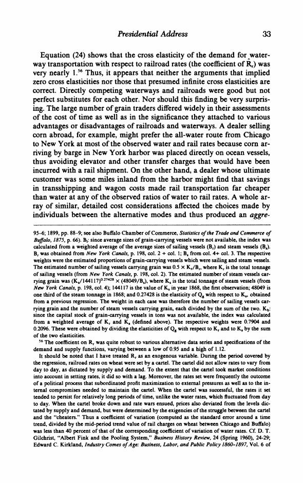
Presidential Address 33
Equation (24) shows that the cross elasticity of the demand for water- way transportation with respect to railroad rates (the coefficient of R.) was very nearly L"56 Thus, it appears that neither the arguments that implied zero cross elasticities nor those that presumed infinite cross elasticities are correct. Directly competing waterways and railroads were good but not perfect substitutes for each other. Nor should this finding be very surpris- ing. The large number of grain traders differed widely in their assessments of the cost of time as well as in the significance they attached to various advantages or disadvantages of railroads and waterways. A dealer selling corn abroad, for example, might prefer the all-water route from Chicago to New York at most of the observed water and rail rates because corn ar- riving by barge in New York harbor was placed directly on ocean vessels, thus avoiding elevator and other transfer charges that would have been incurred with a rail shipment. On the other hand, a dealer whose ultimate customer was some miles inland from the harbor might find that savings in transshipping and wagon costs made rail transportation far cheaper than water at any of the observed ratios of water to rail rates. A whole ar- ray of similar, detailed cost considerations affected the choices made by individuals between the alternative modes and thus produced an aggre-
95-6; 1899, pp. 88-9; see also Buffalo Chamber of Commerce, Statistics of the Trade and Commerce of Buffalo, 1875, p. 66). Be: since average sizes of grain-carrying vessels were not available, the index was calculated from a weighted average of the average sizes of sailing vessels (Br) and steam vessels (B.). Br was obtained from New York Canals, p. 198, col. 2 + col. 1; B, from col. 4+ col. 3. The respective weights were the estimated proportions of grain-carrying vessels which were sailing and steam vessels. The estimated number of sailing vessels carrying grain was 0.5 x K,/B,, where K, is the total tonnage of sailing vessels (from New York Canals, p. 198, col. 2). The estimated number of steam vessels car- rying grain was (K.! 144117)0.27428 x (48049/B,), where K, is the total tonnage of steam vessels (from New York Canals, p. 198, col. 4); 144117 is the value of K, in year 1868, the first observation; 48049 is one third of the steam tonnage in 1868; and 0.27428 is the elasticity of Q. with respect to K,, obtained from a previous regression. The weight in each case was therefore the number of sailing vessels car- rying grain and the number of steam vessels carrying grain, each divided by the sum of the two. Kb: since the capital stock of grain-carrying vessels in tons was not available, the index was calculated from a weighted average of K, and K, (defined above). The respective weights were 0.7904 and 0.2096. These were obtained by dividing the elasticities of Q. with respect to K, and to K, by the sum of the two elasticities.
S6 The coefficient on R, was quite robust to various alternative data series and specifications of the demand and supply functions, varying between a low of 0.95 and a high of 1.12.
It should be noted that I have treated R, as an exogenous variable. During the period covered by the regression, railroad rates on wheat were set by a cartel. The cartel did not allow rates to vary from day to day, as dictated by supply and demand. To the extent that the cartel took market conditions into account in setting rates, it did so with a lag. Moreover, the rates set were frequently the outcome of a political process that subordinated profit maximization to external pressures as well as to the in- ternal compromises needed to maintain the cartel. When the cartel was successful, the rates it set tended to persist for relatively long periods of time, unlike the water rates, which fluctuated from day to day. When the cartel broke down and rate wars ensued, prices also deviated from the levels dic- tated by supply and demand, but were determined by the exigencies of the struggle between the cartel and the "cheaters." Thus a coefficient of variation (computed as the standard error around a time trend, divided by the mid-period trend value of rail charges on wheat between Chicago and Buffalo) was less than 40 percent of that of the corresponding coefficient of variation of water rates. Cf. D. T. Gilchrist, "Albert Fink and the Pooling System," Business History Review, 24 (Spring 1960), 24-29; Edward C. Kirkland, Industry Comes ofAge: Business, Labor, and Public Policy 1860-1897, Vol. 6 of

34 Fogel
gate cross elasticity of demand that was neither zero nor infinity but fairly close to L"
It is difficult to assess Hawke's interesting suggestion that wagon trans- portation was a net complement to both waterways and railroads because the available data relevant to this issue are still so scanty. Wagons served not only as complements to railroads and waterways for freight shipped over long distances but as substitutes for these carriers over short dis- tances. Since a transshipping cost was incurred when transferring freight from wagons to railroads, there was a perimeter surrounding each market within which direct shipment by wagon cost less than shipment by a com- bination of wagons and railroads, even if the railroad rate had been zero. Just how far away from the designated market this perimeter might be lo- cated depends on the ratio of the transshipping cost to the wagon rate as well as on the ratio of the rail rate to the wagon rate. Consequently, a rise in the rail rate would have the effect of both pushing outward the perime- ter that bounds the area in which direct wagon shipment was cheaper (the substitution effect) and reducing the quantity shipped to market per square mile in the area beyond that perimeter (the complementary effect). Whether wagons and railroads were net complements or net substitutes thus depends on whether the substitution or complementary effect was stronger. About all that can be said at present is that it is more likely that the complementary effect would exceed the substitution effect in the post- bellum United States than in England. This is because the ratio of either railroad or waterway to wagon rates was less than 0.1 in the United States. In Hawke's case, however, the ratio of railroad to wagon rates is 0.27 and the waterway to wagon ratio is between 0.42 and 0.56.58
The ratios are relatively high in the English case partly because average English wagon rates were a bit lower than U.S. wagon rates but mainly because the average British railroad and waterway rates were consid- erably higher than those of the late nineteenth-century United States. A variety of factors contributed to the relatively high English waterway and rail rates. One reason frequently mentioned for the high cost of water transport is the small prisms of English canals that kept the vessels narrow and hence thwarted the reduction of freight rates that could have been achieved through increases in the capacity of barges. Another point that deserves emphasis is the short average distance of the English haul, which
The Economic History of the United States, Henry David, et al., eds. (New York, 1961), 85-93; Paul W. MacAvoy, The Economic Effects of Regulation: The Trunk-Line Railroad Cartels and the Interstate Commerce Commission Before 1900 (Cambridge, Mass., 1965), chs. 3-5; Alfred D. Chandler, Jr., The Visible Hand: The Managerial Revolution in American Business (Cambridge, Mass., 1977), pp. 137-43.
The sources of the data for the computation are cited in footnote 55, under variables R,, R, Qg. 57 The word aggregate was emphasized because some of the arguments made for an infinite cross
elasticity really apply to individual shippers. Even if each individual shipper had an infinite cross elasticity of demand, the cross elasticity of the aggregate demand curve could still be in the neighbor- hood of I because of differences among individuals in the slopes of the linear portions of their isoquants as well as in the range over which linearity prevailed.
58 Fogel, Railroads, pp. 71, 107-09; Historical Statistics, p. 733; Hawke, Railways, pp. 62, 86, 180.

Presidential Address 35
c. 1865 was just 33 miles by rail and about 40 miles by canal. But as I have already noted, U.S. rail and waterway hauls in 1890 were from seven to over ten times as long. Consequently, the small physical size of England and the pattern of its internal trade prevented the English from exploiting the potential of the water and rail modes of transportation, which exhib- ited rapidly declining average costs with respect to distance (cf. Figure 3), to the same extent as was possible over the American expanses.59
Railroad Rates and Wagon Rates
Although most of the criticisms of the social saving computations have dealt with waterway rates, some attention has been devoted to railroad rates. O'Brien argued that, because of monopolistic practices in both Eng- land and the United States, the observed railroad rates exceeded marginal cost, so that use of these rates biased downward the social saving compu- tations. Lebergott suggested that the monopolistic pricing policies and profits of American railroads were cloaked by the fact that railroad con- struction was financed with bonds sold at discounts and hence had high yields to maturity. The thrust of this argument is that if adjustments were made for inflated bond rates it would be found that the profit on U.S. rail- road operations in 1890 was well above competitive levels (which implies that rates exceeded marginal costs). The extent of the excess profits is not specified in these critiques, but the suggestion is that it is substantial enough to invalidate the attempts of Fishlow and Hawke to calculate so- cial rates of return and to throw into doubt the relevance of the various social saving calculations.60
The validity of these propositions for U.S. railroads in 1890 can be as- sessed by computing the ratio of the net earnings of railroads to the repro- duction cost of the capital embodied in them, and then comparing this ra- tio to various alternative yields. By using reproduction costs rather than book value, the possibility of inflated capital cost is circumvented. By us- ing net earnings before payment of interest, all returns to capital are cov- ered, including dividends, retained earnings, and interest.
Data collected by the Interstate Commerce Commission indicate that the net operating income of railroads in 1890 (operating revenue less op- erating expenses, including depreciation, and tax accruals) was $330 mil- lion.6' Melville J. Ulmer estimated that the value of the reproducible capi- tal employed in railroad operations in 1890 (value of land and value of capital in such non-railroad operations as hotels were excluded) was $5,827 million, which implies a rate of return of 5.7 percent (330 *. 5,827 - 0.057).62 Fishlow's series on the real net capital stock of railroads in-
9 Hawke, Railways, pp. 61, 86. Cf. the discussion of Figure 1. 60 O'Brien, The New Economic History, pp. 40-45; Lebergott, "United States Transportation," pp.
439-40. Cf. McClelland, "Social Rates," passim. 61 Historical Statistics, p. 737. 62 Melville J. Ulmer, Capital in Transportation, Communications and Public Utilities: Its Formation
and Financing (Princeton, 1960), p. 256.

36 Fogel
dicates a figure for 1890, when converted into dollars of 1890, of $5,446 million.63 Use of Fishlow's data thus implies an 1890 rate of return of 6.1 percent (330 + 5,446 = 0.061). Although it may be appropriate to exclude land values from capital formation and efficiency estimates, it is in- appropriate to do so for profit calculations because competitive firms need to earn the market rate of return on all of their earning assets, including land. Adding $1,495 million for land to the estimates of the reproducible capital derived from Ulmer and Fishlow yields rates of return of 4.5 and 4.8 percent, respectively.' Since the last two figures are below the 1890 yield on industrial common stocks (5.07 percent), the 1890 yield on the stock of utilities (6.03 percent), and the 1890 interest rate on commercial paper (5.62 percent), there seems to be little ground for believing that rail- roads were reaping monopoly profits in that year.65
Suppose, however, that only the reproducible capital stock (as derived from Fishlow) should form the basis for the calculation of the railroad rate of return, and that 5.1 percent (the yield on common stocks) is ac- cepted as the competitive rate of return. By how much would the adjust- ment for monopoly profits increase the estimated social saving of rail- roads? At a rate of 5.1 percent, the competitive profit of railroads should have been $278 million (0.051 x 5,446 = 278) instead of $330 million, which yields $52 million as the monopoly component of profit. Since gross operating revenues in 1890 were $1,052 million, the elimination of the monopoly component of profits would have reduced these revenues to $ 1,000 million, or 95.1 percent of the observed level.' In other words, the elimination of monopoly profit would have reduced freight and passenger rates by an average of 4.9 percent. If the rail freight rates employed in my calculation were reduced by 4.9 percent, the interregional social saving would rise by $4.3 million and the intraregional social saving by $4.8 mil- lion.67 Thus the assumption that one sixth of railroad profits was due to monopoly pricing implies a downward bias in the social saving of $9.1 million. Elimination of this presumed bias would raise the agricultural so- cial saving from 1.78 percent to 1.86 percent of GNP.68 For reasons I have
63 Fishlow, "Productivity," p. 606. The 1890 value for real net capital stock was obtained by inter- polating between Fishlow's 1889 and 1899 figures. The interpolated figure was then converted into dollars of 1890 with the Warren-Pearson price index in U.S. Bureau of the Census, Historical Statis- tics of the United States, 1789-1945. (Washington, D.C., 1949), p. 231.
I Simon Kuznets, National Product Since 1869 (New York, 1946), p. 201. 65 Historical Statistics, p. 1003; Sidney Homer, A History of Interest Rates (New Brunswick, N.J.,
1963), p. 320. 66 Historical Statistics, p. 737. 67 Fogel, Railroads, pp. 42, 72, 86-87; cf. note 50 on pp. 84-85. 68 This calculation gives the order of magnitude of a possible divergence between rates and mar-
ginal costs on a fixed quantity of railroad transportation. One could also compute the effect on the estimated social saving of allowing the quantity transported to respond to the lower rate. If we assume that the elasticity of demand was 1, and that the marginal cost of transportation was approximately constant over the range of increase in transportation service, then the combined effect of a reduction in rates and in quantities carried would be to raise the agricultural social saving from 1.78 to 1.93 per- cent of GNP.

Presidential Address 37
already indicated, however, even this small adjustment is inappropriate. McClelland objected to Fishlow's use of a wagon rate of 15 cents per
ton-mile. "Fishlow's only justification for using that number," he wrote, "is a reference to Taylor's Transportation Revolution." After tracking down Taylor's sources, McClelland concluded that the 15-cent figure "does not inspire confidence." He suggested that 20 cents per ton-mile might be more reasonable, and estimated that such an upward revision would increase Fishlow's freight social saving by $50 million or 48 per- cent.69
Although it is useful to call attention to the need for further research into antebellum wagon rates, it does not follow that Taylor's estimate is wrong merely because it was based on a few citations. Moreover, it is un- likely that the true figure for 1859 would be as high as 20 cents. Some light can be cast on this issue by making use of the 1906 USDA survey of rural wagon transportation in 1,894 counties, which indicated that the average rate per ton-mile (when team, wagon, and driver were hired from com- mercial haulers) was 20.5 cents.70 Since input prices were 53 percent higher in 1906 than they had been in 1859, McClelland's conjecture im- plies that the productivity of wagon transportation increased by 49 per- cent between the two dates.7' So large a productivity increase seems un- likely in light of the fact that 93 percent of all country roads were still unimproved in 1904. Taylor's wagon rate, which implies a 12 percent gain in productivity, is more plausible.72
The issue of antebellum wagon transportation should not be left in such a highly conjectural and unsatisfactory state. Much can be learned about this important but almost wholly unknown aspect of the nineteenth-cen- tury transportation system by turning, as Winifred B. Rothenberg has, to primary sources. Her study of the account books of Massachusetts farmers
69 McClelland, "Railroads," pp. 108-109. 70Fogel, Railroads, p. 56. 71 The total factor productivity index was constructed from the price dual, in the rate-of-change
form. The rate of change in wagon rates implied by McClelland's conjecture is obtained by solving 20.5 = 20ex47. A divisia index of the rates of change in input prices between 1859 or 1860 and 1906 was constructed using wages of farm labor from Historical Statistics, p. 163, and prices of horses and mules from Marvin W. Towne and Wayne D. Rasmussen, "Farm Gross Product and Gross Invest- ment in the Nineteenth Century," in Conference on Research in Income and Wealth, Trends, p. 286. It was assumed that the price of wagons moved with the wholesale price index (Historical Statistics, pp. 200, 201). The weights applied were: labor, 0.44; teams, 0.40; wagons, 0.16. Cf. Fogel, Railroads, p. 72.
If the 1906 wagon rates are projected backward to 1859 on the basis of the index of input prices, we obtain an 1859 wagon rate of 13.4 cents. Even this figure may be too high since the USDA rates were based on the assumption of zero backhauls and because very few farmers hired commerical service but used their own wagons, teams, and labor. Highway engineers argued that the cost of wagon trans- portation to farmers was less than half the commercial rate. An investigation of rates paid to farmers for hauling in central Illinois c. 1906 revealed rates in the neighborhood of 10 cents per ton-mile. The last figure projected back to 1859 by the index of input prices yields a figure of 6.5 cents. Cf. Fogel, Railroads, pp. 107-09.
72 Th procedure followed was described in footnote 71. Taylor's figure implies that wagon rates rose at an annual rate of 0.7 percent.

38 Fogel
reveals perimeters of marketing by wagon between 1750 and 1855 that are wider than has hitherto been presumed. She has also discovered informa- tion on wagon rates that indicates a rise between these dates in the real cost of rural wagon transportation.73 Nor are farm records the only pos- sible sources of information on wagon transportation. Much can also be learned from the records of gristmills, blast furnaces, railroads, and other non-agricultural enterprises that purchased wagon services from farmers.
The uncertainty that surrounds the average wagon rate for 1859 does not really imperil Fishlow's contention that his estimate of the freight so- cial saving represents an upper bound. If one simultaneously increases the wagon rate by a third, as McClelland suggests, and shifts from the as- sumption that E = 0 to E = 0.4, Fishlow's estimate of the freight social sav- ing would fall by one percent. In this case the upward bias due to the as- sumption that E = 0 is slightly greater than the downward bias that McClelland would attribute to a low wagon rate. But E = 0.4 is probably a lower bound on the long-run elasticity of the aggregate transportation de- mand.74 If, as Fishlow argued, e = 1 is a more appropriate figure for the elasticity during the antebellum era, then the upward bias would exceed the potential downward bias by nearly 300 percent.75
THE IMPACT OF RAILROADS ON LONG-TERM ECONOMIC GROWTH
Even if the resource saving of U.S. railroads were relatively small, de- rived (or indirect) effects of the railroads could still be large enough to sustain the view that railroads were indispensable to American economic growth during the nineteenth century, or at least were much more impor- tant than is suggested by the social saving calculations. It is useful to di- vide the derived effects of railroads into two categories. Disembodied ef- fects are those that followed from the saving in transportation costs per se and which would have been induced by any innovation that lowered transportation costs by approximately the amount attributable to rail- roads. Embodied effects are those attributable to the specific form in which railroads provided cheap transportation services. Much effort has been devoted to the investigation of the proposition that the specific in- puts required for railroad construction and operation induced the rise of industries, productive techniques, and management and labor skills that were essential to economic growth. To review this rich literature ade-
" Winifred Rothenberg, "The Marketing Perimeters of Massachusetts Farmers, 1750-1855," mimeo, Brandeis University., 1978.
74 In the long run a rise in the price of transportation would lead to a shift away from transporta- tion-intensive goods as well as to a change in the locus of economic activity. As pointed out below, the Williamson model implies that with increases in the price of transportation of the magnitude in- dicated by Fishlow's social saving, all transportation of agricultural goods from the Midwest to the East could have halted and the United States could have become a net importer of foodstuffs.
7S The data required for these computations come from Fishlow, American Railroads, p. 51, and from McClelland's one-third increase in the wagon rate.

Presidential Address 39
quately would require a separate paper.76 Consequently, this section is limited to a consideration of several attempts to identify substantial dis- embodied effects of railroads that were not covered by the social saving calculations.
Railroad-Induced Economies of Scale
One of the most interesting arguments along this line was set forth by Paul David. He called attention to the possibility that social saving calcu- lations failed to measure the increases in income made possible by long- run declining marginal costs in the transportation-using industries. In the absence of railroads, the scale of operation of such industries would have been lower than it actually was, so that a part of the benefit of railroads was the output gain attributable to a higher scale of operation. This gain, David pointed out, was not originally included in the social saving calcu- lations. He supported his argument with a diagram that showed a gain from economies of scale in the transportation-using industry that was more than ten times as great as the social saving. David did not identify the transportation-using industries to which this diagram might apply, but maintained that such scale effects "remain unexplored, and cannot be ruled out."77
Although further exploration along the lines that David suggests would certainly be useful, it is not likely that adjustments for unmeasured scale effects would significantly alter present estimates of the social saving. This is certainly the case for U.S. agriculture during the nineteenth century since, with the exception of slave plantations, there is no evidence of econ- omies of scale. Suppose, however, that late nineteenth-century agriculture experienced economies of scale similar to those which Engerman and I
76 This work includes, in addition to studies previously cited in connection with the social saving controversy, Stefano Fenoaltea, "Railroads and Industrial Growth, 1861-1913," Explorations in Eco- nomic History, 9 (Summer 1972), 325-51; Wray Vamplew, "The Railways and the Iron Industry: A study of Their Relationship in Scotland," in M. C. Reed, ed., Railways in the Victorian Economy (Newton Abbot, 1969), pp. 33-75; Rainer Fremdling, "Railroads and German Economic Growth: A Leading Sector Analysis with a Comparison to the United States and Great Britain," this JOURNAL, 37 (Sept. 1977), 583-604; and Chandler, The Visible Hand.
77 Quotations of David in this section are from his "Transportation Innovation," pp. 515-19. His diagram, which is reproduced as Part A of Figure 5, makes the "total indirect social benefit" from economies of scale equal to about 97 percent of the f.o.b. value of the end-period output of the trans- portation-using industry. My estimate of the agricultural social saving equals 6.9 percent of the gross farm product of agriculture in 1890. Cf. footnote 79 and Part A of Figure 5.
In a paper published three years after Railroads and American Economic Growth, I noted that the best case for demand-induced economies of scale attributable to railroads was in the Bessemer steel industry. In the absence of the railroad's demand for this type of metal, it is possible that only open- hearth steel would have been available. During the late nineteenth century, open-hearth firms were small scale and produced a more expensive product than Bessemer firms, which were large scale. Taking into account the difference in the cost of production in the two types of firms, the estimated maximum gain in income not already covered by the social saving due to economics of scale in Besse- mer production was just $7.0 million or 0.06 percent of GNP in 1890. See Fogel, "Railroads as an Analogy," pp. 27-30.

40 Fogel
found for the slave South.78 Suppose also that the entire social saving on agricultural freight was charged against the agricultural sector. Then the absence of railroads would have led to a shift of 6.9 percent of inputs from agriculture to transportation (214 . 3107 = 0.069).79 Given a scale coeffi- cient of 1.07, the reduction of the scale of agricultural activities to 0.931 of the level actually attained in 1890 (1 - 0.069 = 0.931) would have reduced agricultural output by 7.4 percent (0.9311 .7 = 0.926; 1 - 0.926 = 0.074). In other words, the unmeasured social saving due to the reduction in the scale of agricultural production is, in this case, $16 million [(0.074 - 0.069) X 3107 = 16]. When expressed as a percentage of GNP, the adjust- ment for the loss attributable to a lower scale of operation in the transpor- tation-using sector raises the agricultural social saving from 1.8 to 1.9 per- cent of GNP.
Even this small adjustment is inappropriate for two reasons. First, as al- ready mentioned, econometric evidence suggests that there were no scale economies in free agriculture until some time after World War I. Second, scale economies, both in the slave South and in post-World War I agricul- ture, were at the level of the firm and therefore would have been captured even in the absence of railroads.80 When scale economies are internal to the firm, increases in the scale of firms are independent of the scale of the industry. Consequently, the relatively small reduction in the scale of agri- culture occasioned by the absence of railroads would have taken the form of a reduction in the number of firms rather than in the scale of each firm.
What explains the discrepancy between David's suggestion that ne- glected scale effects in transportation-using industries might be ten times as great as the social saving and the preceding demonstration that such ef- fects are a tenth or less of the estimated social saving? David did not base his diagram on known features of the agricultural, manufacturing, or service sectors in the United States, Great Britain, or any of the other na- tions for which social savings estimates have been computed. Rather than being applicable to these economies, David's diagram incorporates certain empirically unrealistic assumptions. Chief among these is the assumption that a doubling of output would have led to a 41 percent decline in unit costs. This implies a scale coefficient in the transportation-using sector of
8 The scale coefficient is 1.0645. See Robert W. Fogel and Stanley L. Engerman, Time on the Cross: The Economics of American Negro Slavery, (Boston, 1974), Vol. 2, p. 143. Cf. Gavin Wright, The Political Economy of the Cotton South (New York, 1978), who argues against a scale effect in slave agriculture.
79 My estimate of the agricultural social saving of railroads in 1890 is $214 million. Towne and Rasmussen put farm gross product in the same year at $3,107 million. Consequently, if $214 million of resources had been shifted from agriculture to transportation, the scale of agriculture would have been reduced to 93.1 percent of its actual 1890 level. Fogel, Railroads, pp. 47, 110, 220; Towne and Rasmussen, "Farm Gross Product," pp. 255-312.
1 Cf. Robert W. Fogel and Stanley L. Engerman, "Explaining the Relative Efficiency of Slave Ag- riculture in the Antebellum South," American Economic Review, 67 (June 1977), 275-96; Ralph A. Loomis and Glen T. Bartin, Productivity ofAgriculture: United States 1870-1958, U.S. Dept. of Agri- culture, Technical Bull. No. 1238 (Washington, D.C., 1961), pp. 24-25.
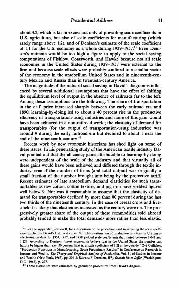
Presidential Address 41
about 4.2, which is far in excess not only of prevailing scale coefficients in U.S. agriculture, but also of scale coefficients for manufacturing (which rarely range above 1.2), and of Denison's estimate of the scale coefficient of 1.1 for the U.S. economy as a whole during 1929-1957.8" Even Deni- son's estimate would be too high a figure to apply to the social saving computations of Fishlow, Coatsworth, and Hawke because not all scale economies in the United States during 1929-1957 were external to the firm and because scale effects were probably confined to a smaller sector of the economy in the antebellum United States and in nineteenth-cen- tury Mexico and Russia than in twentieth-century America.
The magnitude of the induced social saving in David's diagram is influ- enced by several additional assumptions that have the effect of shifting the equilibrium level of output in the absence of railroads far to the left. Among these assumptions are the following: The share of transportation in the c.i.f. price increased sharply between the early railroad era and 1890; learning-by-doing led to about a 40 percent rise in the productive efficiency of transportation-using industries and none of this gain would have been achieved in a non-railroad world; the elasticity of demand for transportables (for the output of transportation-using industries) was around 9 during the early railroad era but declined to about I near the end of the nineteenth century.82
Recent work by new economic historians has shed light on some of these issues. In his penetrating study of the American textile industry Da- vid pointed out that the efficiency gains attributable to learning-by-doing were independent of the scale of the industry and that virtually all of these gains would have been achieved and diffused through the textile in- dustry even if the number of firms (and total output) was originally a small fraction of the number brought into being by the protective tariff. Recent estimates of late antebellum demand elasticities for such trans- portables as raw cotton, cotton textiles, and pig iron have yielded figures well below 9. Nor was it reasonable to assume that the elasticity of de- mand for transportables declined by more than 80 percent during the last two thirds of the nineteenth century. In the case of cereal crops and live- stock it is likely that elasticities increased as the century wore on. The pro- gressively greater share of the output of these commodities sold abroad probably tended to make the total demands more rather than less elastic.
8' See the Appendix, Section B, for a discussion of the procedure used in inferring the scale coeffi- cient implicit in David's f.o.b. cost curve. Griliches's estimation of production functions in U.S. man- ufacturing on data for 1954, 1957, and 1958 yielded scale coefficients that varied between 1.043 and 1.127. According to Denison, "most economists believe that in the United States the number can hardly be higher than, say, 20 percent [that is, a scale coefficient of 1.2] at the outside." Zvi Griliches, "Production Functions in Manufacturing: Some Preliminary Results," in Conference on Research in Income and Wealth, The Theory and Empirical Analysis of Production, Vol. 31 of Studies in Income and Wealth (New York, 1967), pp. 304-8; Edward F. Dension, Why Growth Rates DiOerW (Washington, D.C., 1967), p. 227.
82 These elasticities were estimated by geometric procedures from David's diagram.

42 Fogel
In the case of cotton, econometric estimates indicate that the elasticity of demand was about 50 percent higher after the Civil War than before.83
The point, of course, is that David's diagram should be redrawn to ac- cord with existing empirical information. In Part B of Figure 5, the im- plied scale coefficient is reduced to 1.1, the level of demand is not fixed but increasing, the elasticity of demand remains constant, and the share of transportation in the c.i.f. price is nearly constant in the non-railroad case and declining in the railroad case. Figure 5 shows that when these changes are made, the unmeasured gain in income due to an increase of scale in the transportation-using industry is quite small relative both to the measured social saving and to the output of the transportation-using industry. It follows that the magnitude of the "indirect social benefit" that David inferred from his diagram turned not on general theoretical consid- erations but on specific empirical assumptions implicitly incorporated into that diagram, assumptions that exaggerated the relative magnitude of the unmeasured social saving. So, although David's diagram served the useful purpose of directing attention to the neglected question of railroad-in- duced scale effects in transportation-using industries, it also gave a mis- leading impression of the magnitude of this effect.
DISCUSSION OF PART A OF FIG. 5 The curve labelled LMC-LMC' is the f.o.b. supply curve of the transportation-using industry. It is
downward sloping because of economies of scale, which must be external to the firm. The slope of LMC-LMC' to the left of E, implies that the scale coefficient of the underlying industry production function is 4.2 (cf. the discussion in the Appendix, Section B). David assumes that learning-by-doing will shift LMC-LMC' to LMC*-LMC? but that such a shift will occur only in a railroad world.
The curve tw gives the cost of delivering a unit of output in a non-railroad world and tr gives the cost of delivering a unit of output in a railroad world.
The curve SOS' is the c.i.f. supply curve in a non-railroad world and is obtained by summing LMC- LMC' and tw vertically. The curve SS' is the c.i.f. supply curve in a railroad world and is obtained by summing LMC-LMC' and tr vertically. Note that David has subtracted vf from tw and tr before mak- ing the addition of the relevant curves.
The curve DD' is the long-run market demand curve for transportables (that is, for the output of the transportation-using industry). David argues that in a non-railroad world output would not have expanded beyond OE whereas in a railroad world output would have expanded to OF. Consequently, he argues that the entire shaded area above EF is "the measure of the total indirect social benefit ac- cruing from the introduction of the 'railroad' qua transportation technique." David compares the shaded area over EF with the area fF * vf. "Fogel's actual estimate," he writes, "is over-represented in the figure by the insignificant area fF vf, since he takes the long-run demand for transportables to have been even less price-elastic than the schedule labelled dd' allows." Note that the shaded area over EF is virtually equal to the area designating the f.o.b. value of the output of transportables in the end period (vf- OF).
83 Paul A. David, "Learning by Doing and Tariff Protection: A Reconsideration of the Case of the Ante-Bellum United States Cotton Textile Industry," this JOURNAL 30 (Sept. 1970), 521-601; Robert Brooke Zevin, "The Growth of Cotton Textile Production After 1815," in Fogel and Engerman, The Reinterpretation, pp. 122-47; Robert W. Fogel and Stanley Engerman, "A Model for the Explanation of Industrial Expansion During the Nineteenth Century: With an Application to the American Iron Industry," Journal of Political Economy, 77 (May/June 1969), 306-28; Gavin Wright, "Cotton Com- petition and the Post-Bellum Recovery of the American South," this JOURNAL, 34 (Sept. 1974), 610- 35.

Presidential Address 43
U)~~~~~~~~~~~~~~~~~~~~~~~~~~~~~~~~~~~~~~~~L
Q. 0 . _ U') z > U) ~ ~ ~ ~ ~ ~ ~ ~ ~ ~ ~ U 6
C < 0 0
C:
U) ~~~~~~~~~~~~~~~~~~ 0 Q45~~~~~~~~~~~~~~~ 0 U
0
0~~~~~
-0
*ft 0 0 C) C) C) (~~~~~~~ C)
0
CO~~~~~~~~~~~~~~~~~~~~~~~~~~~C
U-0~~~~~~~~~~~~~~~~~~~~~ : c~~~~~~~~~~~~~~~~~ QO LL~~~~~~~

44 Fogel
DISCUSSION OF PART B OF FIG. 5 I have called this diagram "quasi-empirical" because although it is based on observed U.S. prices,
outputs, and transportation rates, it retains a number of unrealistic assumptions that are necessary to allow for a direct comparison with David's diagram. The most important of these hypothetical as- sumptions is that the scale coefficient in nineteenth-century agriculture between 1850 and 1890 was 1.1. A scale coefficient of 1.1 implies that more than 50 percent of the gain in total factor productivity that Gallman has estimated for this period [cf. Robert E. Gallman, "Changes in Total U.S. Agricul- tural Factor Productivity in the Nineteenth Century," Agricultural History, 46 (Jan. 1972), 2071, is at- tributed here to an increase in scale.
The f.o.b. supply curve can then be derived directly from the price and output measures of crops and livestock set forth in Towne and Rasmussen, "Farm Gross Product" by following the procedure outlined in Appendix, Section B. In order to keep the f.o.b. curve from shifting (again for conve- nience of comparison with David's diagram), it is necessary to assume no changes in total factor pro- ductivity other than those attributable to scale and to keep input prices constant. Then the observed price and output point for 1850 ($55.4 and 24.2 million tons) and the assumed scale coefficient locate the f.o.b. curve. The observed output in 1890 (83.2 million tons) and the f.o.b. curve yields the as- sumed actual price of $49.2 in 1890. The price per ton for 1850 was obtained by dividing the value of crops and livestock by the tonnage. Only crops and livestock entering farm gross product are in- cluded. Forest products were excluded from both the numerator and denominator. The prices are in constant dollars of 1910-14.
The curve marked R-Rr gives the estimated average actual dollar value of transportation required to deliver a ton of agricultural output from the f.o.b. point to the c.i.f. destination. The 1850 point was estimated by assuming that the ratio of the observed average annual price of corn in Cincinnati to the corresponding price in New York measured the ratio of the f.o.b. to c.i.f. prices [computed from Ar- thur Harrison Cole, Wholesale Commodity Prices in the United States 1700-1861, Statistical Supple- ment (Cambridge, Mass., 1938), p. 314]. The 1890 point was estimated in a similar manner using the ratio of the Wisconsin and New York prices of wheat as reported in Williamson, Late Nineteenth- Century, p. 259. The remainder of the curve was interpolated log-linearly. Such interpolation does not necessarily imply that increases in the productivity of railroads were a function of the scale of agricul- ture; an incidental temporal correlation between agricultural output and railroad productivity is suf- ficient.
The curve marked R-Rw gives the price of delivering a ton of agricultural output from the f.o.b. point to the c.i.f. destination in a non-railroad world. The 1890 point was obtained by multiplying the 1890 price in a railroad world by 1.87 (see Table 2 above). It was assumed that the 1850 prices of transporting a ton of agricultural output were identical in the railroad and in a non-railroad world, since over 90 percent of the transportation of agricultural commodities in that year went by means other than railroads (cf. Fogel, Railroads, pp. 4-5; Fishlow, American Railroads, pp. 18-19). However, choosing a point slightly above $32.4 for 1850 would have little effect on the analysis. The remainder of the Rw curve was interpolated log-linearly between the 1850 and 1890 points.
The curve marked c.i.f.-c.i.f.(r) is obtained by the vertical addition of the f.o.b. and R-Rr curves. Similarly, the c.i.f.-c.i.f.(w) curve is the result of the vertical addition of the f.o.b. and R-R, curves.
The constant elasticity demand curves for 1850 and 1890 are located by the outputs and c.i.f. prices for the respective years and the assumed elasticities, which in both cases were put at 0.8.
Three shaded areas are shown in the diagram. The rectangle marked I is the estimated social saving and is given by the 1890 difference between the Rw and Rr curves ($14.51) and the amount of output (32.2 million tons) shipped by railroad. Note that only about 39 percent of farm gross product was shipped by rail (cf. Fogel, Railroads, pp. 74, 76). The rectangle marked II is the scale effect induced in agriculture by the railroad. It is the additional cost of producing 71 million tons of output because of the reduced scale of production (71.0 x $0.71 = $50). The triangle marked III is the overestimate of the social saving due to the assumption that e = 0.
Thus, the scale effect is about 11 percent of the measured social saving or about 1.2 percent of gross farm product. Its omission is more than offset by the upward biases due to the assumption that e = 0.
It is worth noting that an increase in the elasticity of demand will have effects that go in opposite directions. The greater E, the greater the upward bias in the social saving estimate due to assuming that e = 0. But the greater e, the greater the downward bias in the social saving due to neglect of the scale effect. Given the magnitude of the scale effect, however, increasing e cannot reverse the finding that the upward bias exceeds the downward bias.
Note also that this diagram does not allow for the substantial decline in the long-run cost of water- way transportation associated with the increased volume of output that was indicated in the second part of this paper.

Presidential Address 45
Railroad-Induced Structural Changes
The social saving model is an effective tool in the analysis of the com- parative efficiency of transportation systems. When the social saving esti- mate is built up road by road, as Fishlow did, or commodity by com- modity, as Hawke and Metzer did, it is possible to obtain a fairly fine- grained picture of the relative advantages of different carriers under a va- riety of circumstances. On the other hand, the social saving model is poorly adapted to the analysis of the impact of railroads on the structure of economic activity. It is, for example, possible that "even a social saving as small as one fourth of I percent of national income would have ended all or most" production of agricultural surpluses in the North Central states.' The social saving model contains no mechanism for assessing ei- ther this possibility, or the possibility that a small social saving could have led to dramatic shifts in the balance between agriculture and manufactur- ing or between investment goods and consumer goods. The social saving model cannot answer these and other structural questions because it has only one sector besides transportation.
The Williamson model transcends this limitation by allowing, in addi- tion to transportation, two production sectors in the Midwest and one in the East.85 It also contains mechanisms through which one could analyze the influence of railroads on the pattern of interregional trade as well as on the sectoral allocations of labor and capital. Charles Kahn has been in- vestigating the properties of the Williamson model and it-was my original intention to present his findings as an appendix to this paper. Kahn's in- vestigation, however, has opened up so many interesting issues that it has burst the bounds of an appendix and deserves to be elaborated in a sepa- rate paper. Meanwhile, I would like to offer some brief observations on the Williamson model that draw heavily from Kahn's preliminary find- ings and also from some unpublished notes that Claudia Goldin has gen- erously made available to me.86
Although Williamson attributes the social saving computed from his model to railroads, it is actually the social saving due to all improvements in transportation and distribution between 1870 and 1890. He did not mea- sure the cost of railroad transportation from farms to eastern markets di- rectly but instead used the difference in the spot prices of wheat in Iowa and New York as a proxy. Throughout the period from 1870 and 1890, however, most of the wheat shipped eastward from Chicago, Minneapolis, Duluth-Superior, and Milwaukee went by Great Lakes vessels.87 Con- sequently, the price differential used by Williamson as a measure of the decline in rail transport costs was quite heavily influenced by the rapid fall in grain transportation rates on the Great Lakes and, to a significant degree, by the decline in grain rates on the Erie Canal, and by the decline
8' Fogel, Railroads, p. 21. 85 See Williamson, Late Nineteenth-Century American Development, ch. 9. ' Several of the points which follow were also raised in McCloskey, "New Model History." 87 U.S. Bureau of Statistics, Monthly Survey, pp. 1964-67; Tunnell, "Statistics," pp. 30-59.

46 Fogel
in elevator charges, drayage charges, insurance charges, and other mar- keting costs. The differential in spot prices also, of course, was influenced by short-term disequilibria in both the New York and Iowa markets. Since the spread between the "gold points," or more properly "the wheat points," was quite a high percentage of the Iowa farm price, the dis- equilibrium component of the observed prices could be quite large. Since Iowa was on the outermost fringes of the wheat belt in 1870, it is likely that its spot price was subject to much greater year-to-year variance at the beginning of the period than was that of farms near the center of wheat production, and that the rate of decrease in the Iowa-New York differen- tial would be much greater than that in the differential between New York and a more central location. The switch from a "railroad" social saving to a social saving due to all increases in transportation and distri- bution productivity between 1870 and 1890 is not an error but a rather in- teresting innovation.
It appears that there were errors either in the original computation (per- haps in the program) or in the data sets and simulation results reported by Williamson in his appendices, and that these errors led to an over- statement of the 1890 social saving by about 60 percent. Kahn's efforts to replicate Williamson's results yielded an 1890 social saving not of 21 per- cent but of 12.8 percent, which is still, of course, a relatively large figure. The estimated social saving also turns out to be substantially influenced by a number of unrealistic assumptions built into the model. One of these is the assumption that it was possible to more than double the amount of service provided by the transportation sector without any diversion of in- puts from other sectors. In other words, increases in the output of trans- portation result in a net increase in GNP by the same amount, since there is either no alternative cost for the extra resources required to increase transportation output, or because no additional resources are required. When Kahn amends the model to allow for the alternative cost of the in- creases in transportation services, the 1890 social saving declines from 12.8 to 6.7 percent of GNP.
The social saving in 1890 generated by Williamson's model poses a dif- ficult index number problem, since the magnitude of the estimate relative to GNP varies considerably with the selection of the prices in which to evaluate real GNP and sectoral output (1870, current-year, or counter- factual current-year). The magnitude of the social saving in particular years is also affected by whether or not one smoothes the series of spot wheat prices to eliminate variations in the inferred cost of transportation that are due to local disequilibria. This exercise suggests that a substantial proportion of the remaining social saving is due to unusual conditions in the extreme years. It would be quite premature, however, to draw the con- clusion that appropriate revisions of the Williamson model will necessar- ily result in a rather small social saving attributable to productivity changes in the transportation sector. Not all of the plausible adjustments are in the direction of reducing the social saving. If, for example, one per-

Presidential Address 47
mits greater flexibility in the intersectoral movement of labor and capital than Williamson allowed, the social saving increases somewhat.
Perhaps the two most interesting of Kahn's preliminary findings are that "dynamic" or time-path effects may be a considerable part of the so- cial saving, and that a small social saving could result in large changes in the patterns of trade. To determine what part of the social saving in 1890 was due to markups in that year and what part was due to the social sav- ing in previous years, Kahn re-ran the simulation under the constraint that transportation costs (Williamson's ZA and ZI) did not increase to counterfactual levels until 1890. This run yielded a social saving of 3.7 percent of GNP instead of the 6.7 percent figure obtained when the social saving is allowed to rise continuously (and after an adjustment for the fact that transportation had an alternative cost). It thus appears that the dy- namic considerations could account for close to half of the social saving.88
The sensitivity of trading patterns to small social savings turns up in both the original Williamson model and in Kahn's various alternative simulations. In all of the models there are years in which the United States is a net importer of grains. Similarly, exports and imports between the East and the West sometimes reverse directions. From the strictly modeling viewpoint, this result poses the question of how to deal with prices that are sometimes exogenous and sometimes endogenous (Wil- liamson assumed that grain prices in the East were fixed in Liverpool).89 The more intriguing question opened up by this finding is the possibility that regional trading patterns, economic alliances, and political alliances may have been affected profoundly by processes that had only a small im- pact on the level of GNP.
The exciting new lines of research opened up by the Williamson model clearly deserve to be followed up. But such a pursuit should not be coun- terposed to further analyses based on the social saving model. The social saving model is, as I have suggested, quite a useful device for analyzing the relative importance of various applications of a given innovation, or the incremental gain in the productivity attained by substituting one in- novation for another when such substitution appears possible. Von Tun- zelmann's considered and inventive application of the social saving model
88This result obtains when, following Williamson, the social saving is computed in 1870 prices. If 1890 prices are used, the dynamic effects are nearly wiped out. The sensitivity of the dynamic effects to the prices employed serves to re-emphasize the seriousness of the index number problem alluded to above.
89 Some aspects of this problem are addressed by Frank Lewis ("Explaining the Shift of Labor from Agriculture to Industry in the United States: 1869 to 1899," unpublished Ph.D. dissertation, University of Rochester, 1976), who stressed the unrealism of models in which the United States can import agricultural goods at the same price at which it exports them. Lewis uses a simpler framework than Williamson's, allowing him to have separate international buying and selling prices for wheat (the difference being the trans-Atlantic shipping costs). For intermediate prices, demand is the in- elastic domestic demand rather than the elastic international demand. Including this international transportation wedge reverses many conclusions about the effects of changes in agricultural produc- tivity. In Williamson's model, declining domestic transportation costs act in many respects like in- creases in agricultural productivity. Thus, allowing a Lewis-like refinement in the Williamson model could well increase the transportation social saving.
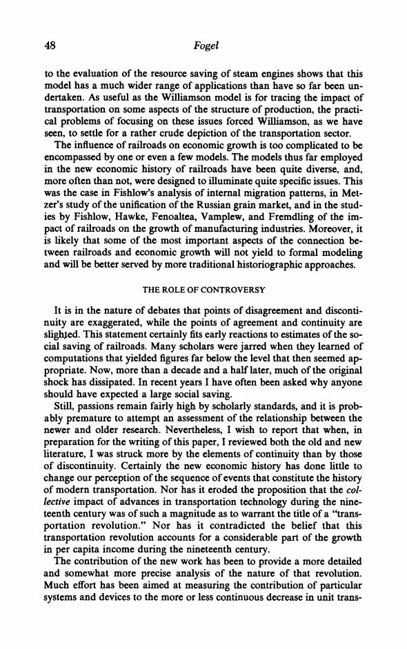
48 Fogel
to the evaluation of the resource saving of steam engines shows that this model has a much wider range of applications than have so far been un- dertaken. As useful as the Williamson model is for tracing the impact of transportation on some aspects of the structure of production, the practi- cal problems of focusing on these issues forced Williamson, as we have seen, to settle for a rather crude depiction of the transportation sector.
The influence of railroads on economic growth is too complicated to be encompassed by one or even a few models. The models thus far employed in the new economic history of railroads have been quite diverse, and, more often than not, were designed to illuminate quite specific issues. This was the case in Fishlow's analysis of internal migration patterns, in Met- zer's study of the unification of the Russian grain market, and in the stud- ies by Fishlow, Hawke, Fenoaltea, Vamplew, and Fremdling of the im- pact of railroads on the growth of manufacturing industries. Moreover, it is likely that some of the most important aspects of the connection be- tween railroads and economic growth will not yield to formal modeling and will be better served by more traditional historiographic approaches.
THE ROLE OF CONTROVERSY
It is in the nature of debates that points of disagreement and disconti- nuity are exaggerated, while the points of agreement and continuity are slighted. This statement certainly fits early reactions to estimates of the so- cial saving of railroads. Many scholars were jarred when they learned of computations that yielded figures far below the level that then seemed ap- propriate. Now, more than a decade and a half later, much of the original shock has dissipated. In recent years I have often been asked why anyone should have expected a large social saving.
Still, passions remain fairly high by scholarly standards, and it is prob- ably premature to attempt an assessment of the relationship between the newer and older research. Nevertheless, I wish to report that when, in preparation for the writing of this paper, I reviewed both the old and new literature, I was struck more by the elements of continuity than by those of discontinuity. Certainly the new economic history has done little to change our perception of the sequence of events that constitute the history of modern transportation. Nor has it eroded the proposition that the col- lective impact of advances in transportation technology during the nine- teenth century was of such a magnitude as to warrant the title of a "trans- portation revolution." Nor has it contradicted the belief that this transportation revolution accounts for a considerable part of the growth in per capita income during the nineteenth century.
The contribution of the new work has been to provide a more detailed and somewhat more precise analysis of the nature of that revolution. Much effort has been aimed at measuring the contribution of particular systems and devices to the more or less continuous decrease in unit trans-

Presidential Address 49
portation costs during the nineteenth century.' The design of. appropriate measures of productivity and the explanation of changes in productivity have required a detailed analysis of the performance characteristic of the large array of devices employed in each of the modes of transportation. The demands of measurement have also required a search for bodies of data not previously assembled by transportation historians as well as a careful reconsideration of the reliability and relevance of those series that had been assembled and utilized in earlier studies.
Much time was devoted to such tedious tasks as the determination of equivalences between various weights and measures, assessment of the homogeneity or non-homogeneity of commodities and services to which particular price series pertained, assessment of the completeness of cov- erage in various data sources, and construction of new time series from underlying company records, trade association reports, and censuses.
It would be surprising if the many thousands of hours of work spent on such tasks did not produce new insights. In this paper I have alluded to a number of these. Here I wish to summarize briefly the most important findings:
1. It is a misleading oversimplification to identify wagons, waterways, and railroads with a sequence of temporal stages in which each was pre- dominant or to suggest that railroads replaced waterways because water- ways had reached the limit of their technological capacity. Nor is it cor- rect to describe waterways as more efficient carriers than wagons, and railroads as more efficient than waterways. The transportation system that evolved during the nineteenth century embraced all three modes. The quantities of service delivered by each mode increased throughout the nineteenth century, although at unequal rates. Each mode was more pro- ductive than the other two in some domain, and this pattern of specialized pre-eminence continued to the end of the nineteenth century.9'
2. Nineteenth-century innovations in transportation techniques served to reduce unit transportation costs mainly over medium and long dis- tances. Unit transportation costs of freight were usually as high (or higher) over short distances by railroads and waterways as they were by wagon. Spectacular reductions in short-haul transportation had to await the perfection of motor vehicles.
3. Waterways and railroads were good, but not perfect, substitutes for each other. Waterways generally had an advantage over railroads in the carrying of bulky, low-value items over long distances. Railroads had an advantage in carrying high-value items over both medium and long dis- tances, and in carrying bulky, low-value items over medium distances.
I As Fishlow ("Productivity," pp. 642-44) has pointed out, the social saving can be interpreted as a measure of total factor productivity. Cf. Fogel and Engerman, The Reinterpretation, p. 102.
I' The specialized pre-eminence of waterways during the last half of the nineteenth century has been neglected by economic historians because of a preoccupation with canals, which were, in many cases, superseded by railroads, and which only provided a small share of total waterway transporta- tion. Cf. the Appendix, Section A.

50 Fogel
For most categories of freight, however, these edges were much smaller than the edge that either waterways or railroads enjoyed over wagons for hauls of medium and long distances.
4. The crux of the transportation revolution of the nineteenth century was the substitution of low-cost water and railroad transportation for high-cost wagon transportation. This substitution was made possible by a dense network of waterways and railroads. Whereas the combination of waterways and railroads provided the most efficient substitute, in most cases so far studied either by itself would have provided most of the re- source saving effected by the combination. Railroads were indispensable, however, in regions where waterways were not a feasible alternative.
5. There is no uniform answer to the question of whether the resource gain brought about by railroads or by waterways was the greater. The an- swer varies with country or region and time period. In mountainous coun- tries, such as Mexico, railroads were the only effective substitutes for wagons. In the United States before 1850 the contribution of waterways may have exceeded that of railroads. After 1860 or 1870 the railroad con- tribution was probably greater, not because the waterway potential for in- creased productivity had run its course, but because the marginal cost of transportation with respect to the density of the network was higher for waterways than for railroads.
6. Productivity advanced at a brisk pace for both waterways and rail- roads throughout the nineteenth century. Douglass C. North estimated that total factor productivity on ocean freight increased at an annual rate of 3.3 percent over the period from 1814 to 1860. C. K. Harley's analysis of ocean vessels over the period from 1873 to 1890 indicated annual rates of productivity growth of 2.2 percent for sailing vessels and 3.1 percent for steamships.92 In the case of inland waterways, Erik F. Haites, James Mak, and Gary Walton found that the annual rate of increase in the total factor productivity of Mississippi steamboats was 6.5 percent between 1815 and 1830 and 2.4 percent between 1830 and 1860. We are still without a study of total factor productivity on U.S. inland waterways during the last third of the nineteenth century. The course of freight rates on the Great Lakes, however, suggests a rapid increase in productivity on that waterway. The freight on wheat between Chicago and Buffalo (in constant dollars) de- clined at an annual rate of 2.6 percent between 1868 and 1898. Since real wages (the main cost component of both waterway services and the con- struction of vessels) were rising, it is probable that total factor productiv-
92 Douglass C. North, "Sources of Productivity Change in Ocean Shipping," Journal of Political Economy, 76 (Sept./Oct. 1968), 965. Charles K. Harley, "The Shift from Sailing Ships to Steamships, 1850-1890: A Study in Technological Change and Its Diffusion," in Donald N. McCloskey, ed., Es- says on a Mature Economy (London, 1971), p. 228. The rate of growth in total factor productivity for freight transported by sailing ships can be computed from Harley's essay. The rate of productivity growth for freight carried by steamships, however, requires information on the growth of productivity in the building of steamships, which was not reported. I am grateful to Professor Harley for supplying the needed information.

Presidential Address 51
ity increased more rapidly on the Great Lakes during this period than on railroads.93 In the case of railroads, Fishlow's estimates show that total factor productivity gained at annual rates of 5.7 percent between 1839 and 1859, and 2.6 percent between 1859 and 1910.9' The productivity studies of the past decade, then, suggest that the technological advances of water- way carriers of freight-on the Mississippi at least up to 1860, and on the Great Lakes and ocean routes throughout the century-were quite rapid, even if they did not always match railroad advances.
7. The capacity of various nations and regions to exploit technological possibilities of waterways and railroads depended on the nature of their demand for transportation. Average railroad and waterway rates were higher in England than in the United States because the English economy required hauls mainly of short-to-medium distances, whereas the U.S. hauls were mainly medium-to-long distances.
It is worth noting that although some of these points were developed in the original social-saving studies, not all of them were. And some points vaguely adumbrated in the original studies emerged clearly only in the course of the subsequent debate. I stress this point, because some observ- ers of the debate have misunderstood it. They have interpreted the sharp disagreements among the cliometricians as evidence of the failure of so- cial science methodology, and particularly of quantitative methods, in his- tory.
There is in this view a confusion between artistic and scientific proc- esses. A painting, a concerto, a novel, and even certain types of histories can be the perfect creation of a single individual during a relatively brief period of intense activity. Such artistic works normally have a highly per- sonal quality. Scientific creations, however, are usually protracted over long periods, approach perfection quite gradually, and involve the efforts of a large number of investigators. The social saving controversy has dem- onstrated the great complexity of the analysis of the developmental im- pact of railroads, the wide range of issues that need to be pursued, the large amounts of data that must be retrieved, and the many pitfalls that may be encountered in the analysis of these data. Such problems are re- solved through collective effort, one aspect of which is the intense debate over the significance and validity of successive contributions.
The various criticisms of the social saving computations served to iden- tify areas in which the initial results were either incorrect, incomplete, or inadequately supported. Quite often the objections were of a conjectural nature, even though they were expressed in a rhetoric that suggested a high degree of certitude. Whatever the rhetoric, the list of criticisms con-
93 Erik F. Haites, James Mak, and Gary M. Walton, Western River Transportation: The Era of Early Internal Development, 1810-1860 (Baltimore, 1975), pp. 183-84. Interestingly enough, Haites, Mak, and Walton found that the total factor productivity of flatboats increased at an annual rate of 3.8 to 4.4 percent between 1815 and 1860 (ibid., p. 76). Fishlow ("Productivity," p. 626) indicates that rail- road total factor productivity rose at an annual rate of 2.3 percent between 1870 and 1900.
94 Fishlow, "Productivity," p. 626.

52 Fogel
stituted the agenda for subsequent rounds of research. The results of the interaction between the investigators and the critics have been a gradual deepening of the analysis, an improvement of estimating procedures, and the searching out of additional, or more reliable, bodies of evidence bear- ing on the points at issue. Rather than being a sign of the failure of the cliometric method, the controversy is a sign that the method is working.
Appendix
A. THE METHOD OF ESTIMATING TON-MILES OF WATER TRANSPORTATION AND THE AVERAGE LENGTH OF A WATER
HAUL IN 1889
I have employed Barger's estimates of the total ton-miles and average distances of hauls in 1889 for the coastwise and intercoastal routes. The corresponding estimates for the Great Lakes and for other inland routes, however, are too low. For the Great Lakes, Bar- ger assumed an average haul of 578 miles, which is well below the estimates of C. H. Keep, secretary of the Lake Carriers' Association, and other experts on water shipping who wrote on the subject in the 1890s. Based on statistics for the Detroit River (through which over three quarters of all the Great Lakes traffic passed in 1889) or the Soo Canal, they put the average length of a haul between 700 and 750 miles (Tunnell, "Statistics," p. 12; New York Canals, p. 197).
Barger apparently misinterpreted the data in Census of Transportation 1890, Part II, pp. 395-465, which deals with transportation on the Mississippi River system. The 2.6 billion ton-miles that he attributed to the system's total movement of coal and lumber refer only to 4.0 million tons of coal shipped from five cities (ibid., p. 408), which means that the av- erage haul on these coal shipments was 658 miles. Since more than half of all lumber ship- ments on the Mississippi originated in northern Wisconsin or Minnesota, and since 17 per- cent of all lumber originating on the upper Mississippi (as defined by the census) was destined for the lower Mississippi (ibid., p. 440; cf. pp. 408-09), it appears likely that the average hauls on lumber and coal were about the same.
Barger put the average haul of all other commodities on the Mississippi, as well as all other rivers and canals, at 40 miles. He took this last figure from data obtained from the Army Engineers for the 1920s. But between 1889 and the 1920s, the pattern of traffic on rivers and canals had changed drastically, with much of the long-distance haulage having been abandoned. During the 1 890s the Mississippi steamboat packets engaged in the long- distance transportation of agricultural products went out of business. After the turn of the century, long-distance towing of barges carrying agricultural products between St. Louis or Cincinnati and New Orleans was also abandoned. By the time of World War I, only local traffic in agricultural products on the Mississippi system could compete successfully with railroads. See U.S. Department of Agriculture, Bulletin No. 71, "Inland Boat Serv- ice," by Frank Andrews, (December 19, 1914), pp. 7-9; cf. U.S. Engineer Dept., Board of Engineers for Rivers and Harbors (War Dept.), Transportation in the Mississippi and Ohio Valleys, Transportation Series No. 2 (Washington, D.C., 1929), ch. 3.
In developing his estimate of ton-miles for the other-inland-routes category, Barger did not include an adjustment for the double counting of tonnage which occurs when freight is carried on more than one waterway (for example, on the Great Lakes and on the St. Mary Falls Canal). Suchl duplication is not a problem if one merely desires to measure ton-miles. It is a problem, however, if one also needs to estimate tons originated (tons not having had a previous line-haul on a connecting waterway) and the average haul of tons originated, as is the case in this paper.

Presidential Address 53
The revised estimates, presented in Appendix Table 1, omit transportation on the riv- ers that were not part of the Mississippi system, so both the totals for tonnage and ton- miles may be understated, but the likely error is small. The revised estimate of the total ton-miles of contiguous domestic water transportation for 1889 is 49.7 billion, which ex- ceeds Barger's estimate (the sum of the first 4 columns of his Table H-1) by 13.9 billion.
APPENDIX TABLE I ESTIMATED TON-MILES OF WATER TRANSPORTATION, TONS ORIGINATED,
AND AVERAGE LENGTH OF A HAUL IN 1889
1 2 3 Tons A verage Haul Ton-miles
System Originated (miles) (109) (106)
1. Coastwise 11.9 1,226 14.6 2. Intercoastal 0.307 6,185 1.9 3. Great Lakes (domestic) 25.3 700 17.7 4. Mississippi system 29.4 478 14.1 5. Canals 9.54 143 1.4
6. Totals 76.5 49.7 7. Average haul per ton originated 49,700 + 76.5 = 650 miles
Sources and Notes: Lines 1 and 2: Barger, Transportation Industries, pp. 254-55. Line 3: Col. 1. ibid.; col. 2 Tunnell, "Statistics," p. 12; New York Canals, p. 197. Line 4: Col 1, Barger, Transportation In- dustries, pp. 254-55; col. 2, computed from data in Census of Transportation 1890, pp. 408, 439-40 on the assumption that lumber had the same average haul as coal, and that the average haul on all com- tnodities except coal and lumber was 200 miles. Line 5: Cols. 1 and 2, Census of Transportation 1890, Part II, pp. 474-79. Tonnage on ship canals and on canalized rivers were excluded. Since such canals were connecting links between other waterways (such as between Lake Superior and Lake Michigan), this tonnage has already been attributed to some other waterway. The exclusion of the ton-miles of these canals from col. 3, however, imparts a downward bias into the average haul. About 60 percent of the tonnage and 70 percent of the ton-miles entered in line 5 are attributable to the New York State canals, the data for which are reported in New York Canals, pp. 181-83. For the other canals, I as- sumed that the ratio of the average length of a haul to the "averaging working length" for the New York canals (0.686) also prevailed on other canals. "Averaging working length" of the New York ca- nals was defined as the length of each canal in the system, weighted by that canal's share in the total tonnage. An analogous definition was used for the other canals. Thus 0.686 times the "average work- ing length" of the other canals yielded the estimated average haul on these canals. It should be noted that about half of the tonnage on the New York canals originated elsewhere, so that the sum of col. 1 tends to overstate tons originated. This will impart a downward bias on the estimated average haul (in line 7), but this double counting does not bias the average haul on canals or the total ton-miles on canals.
B. THE METHOD OF ESTIMATING THE SCALE COEFFICIENT IMPLICIT IN DAVID'S F.O.B. SUPPLY CURVE
David's discussion of the diagram is quite terse, and not all of the specifications of his f.o.b. supply curve, which he identifies as LMC-LMC', are stated explicitly. However, for reasons indicated in the text, it is clear that the economies of scale involved here must be external to the firm, so that LMC-LMC' must be the industry-wide supply curve. Since the LMC-LMC' curve is the locus of the long-run equilibrium points of the individual firms summed horizontally, LMC-LMC' must also be the locus of the average costs of the indi- vidual firms summed horizontally. This is because in the long run (that is, a period long enough for the individual firm to vary its plant size but not the scale of the industry) the

54 Fogel
individual firms will adjust their plant size so as to produce at the point at which long-run marginal cost and long-run average cost intersect, and this will be true at every industry- wide scale of operation. Since movements along the LMC-LMC' curve are due to changes in the scale of the industry, the LMC-LMC' curve will be of the form:
Ci/Qi - Q (I/X) f(PR)
which follows from the total cost curve,
Ci - Qil/xf(P),
where Ci is the total cost of the industry-wide output in period i, Q is the industry-wide output in period i, x is the scale coefficient (the sum of the output elasticities of the indus- try-wide production function), and pj is a vector of the prices of inputs.
Measurements performed on David's diagram indicate that when Q2 + = 2, (C2 + Q2) + (C, + Q.) = 0.59. Hence we may write:
C2
Q2 C2 Q I C2 92 C2 X =- xO.5 =O.59, C IC, Q2 C1 Q.
or = 1.18. CI
Since the pj are presumed to remain constant, it follows that:
c2 (Q2x
or 1.18 =2'x and x = 4.2.