Embed Size (px)
Citation preview
Economic Implications of Alternative Allocation Schemes
for Emission Allowances
Christoph BöhringerCentre for European Economic Research (ZEW)
P.O. Box 10 34 43, D-68034 Mannheim, Germany
University of Heidelberg, Department of Economics, Germany
E-mail: [email protected]
Andreas LangeCentre for European Economic Research (ZEW)
P.O. Box 10 34 43, D-68034 Mannheim, Germany
AREC, University of Maryland, USA
E-mail: [email protected]
Downloadable Appendix(ftp://ftp.zew.de/pub/zew-docs/div/allocation.pdf)
Appendix A: Algebraic Model Summary I
Appendix B: Sensitivity Analysis XII
I
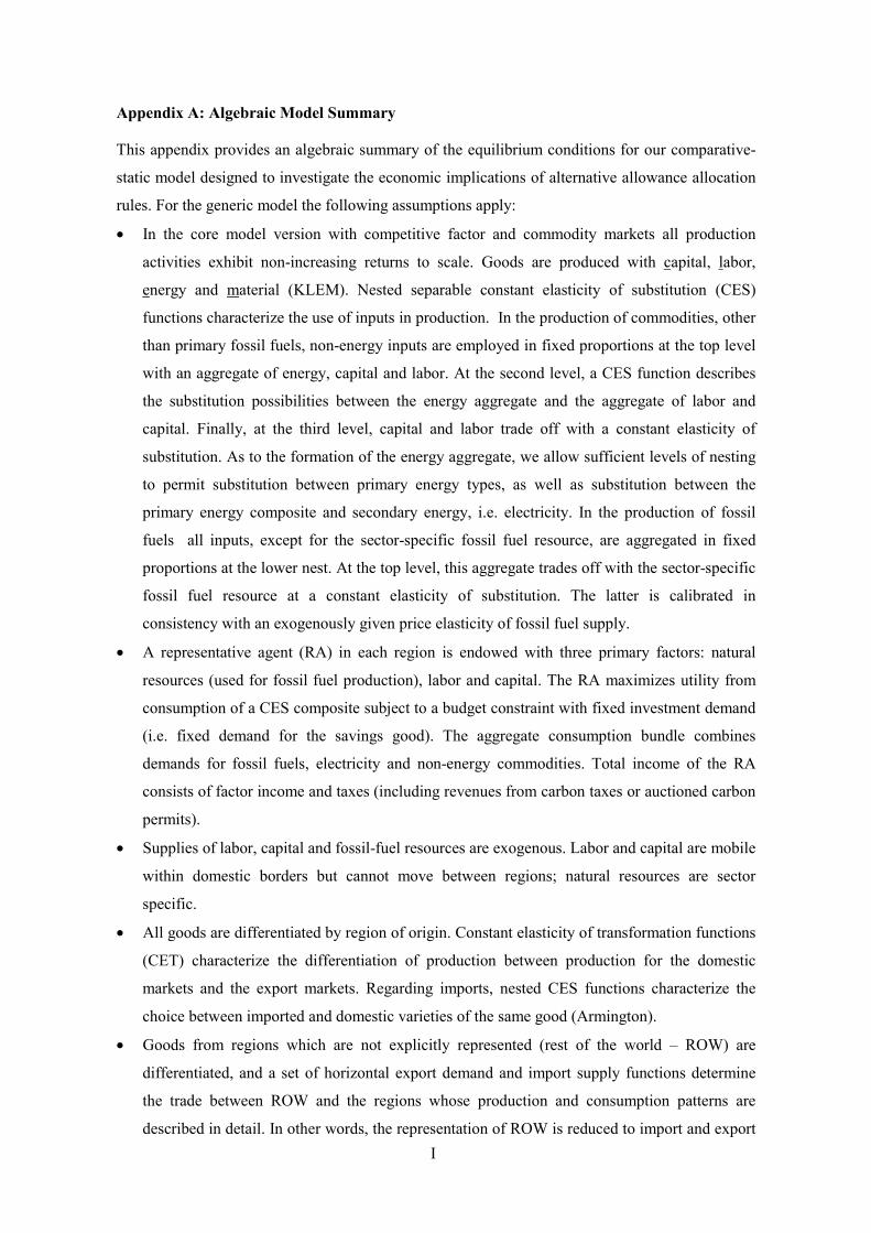
Appendix A: Algebraic Model Summary
This appendix provides an algebraic summary of the equilibrium conditions for our comparative-
static model designed to investigate the economic implications of alternative allowance allocation
rules. For the generic model the following assumptions apply:
� In the core model version with competitive factor and commodity markets all production
activities exhibit non-increasing returns to scale. Goods are produced with capital, labor,
energy and material (KLEM). Nested separable constant elasticity of substitution (CES)
functions characterize the use of inputs in production. In the production of commodities, other
than primary fossil fuels, non-energy inputs are employed in fixed proportions at the top level
with an aggregate of energy, capital and labor. At the second level, a CES function describes
the substitution possibilities between the energy aggregate and the aggregate of labor and
capital. Finally, at the third level, capital and labor trade off with a constant elasticity of
substitution. As to the formation of the energy aggregate, we allow sufficient levels of nesting
to permit substitution between primary energy types, as well as substitution between the
primary energy composite and secondary energy, i.e. electricity. In the production of fossil
fuels all inputs, except for the sector-specific fossil fuel resource, are aggregated in fixed
proportions at the lower nest. At the top level, this aggregate trades off with the sector-specific
fossil fuel resource at a constant elasticity of substitution. The latter is calibrated in
consistency with an exogenously given price elasticity of fossil fuel supply.
� A representative agent (RA) in each region is endowed with three primary factors: natural
resources (used for fossil fuel production), labor and capital. The RA maximizes utility from
consumption of a CES composite subject to a budget constraint with fixed investment demand
(i.e. fixed demand for the savings good). The aggregate consumption bundle combines
demands for fossil fuels, electricity and non-energy commodities. Total income of the RA
consists of factor income and taxes (including revenues from carbon taxes or auctioned carbon
permits).
� Supplies of labor, capital and fossil-fuel resources are exogenous. Labor and capital are mobile
within domestic borders but cannot move between regions; natural resources are sector
specific.
� All goods are differentiated by region of origin. Constant elasticity of transformation functions
(CET) characterize the differentiation of production between production for the domestic
markets and the export markets. Regarding imports, nested CES functions characterize the
choice between imported and domestic varieties of the same good (Armington).
� Goods from regions which are not explicitly represented (rest of the world – ROW) are
differentiated, and a set of horizontal export demand and import supply functions determine
the trade between ROW and the regions whose production and consumption patterns are
described in detail. In other words, the representation of ROW is reduced to import and export
II
flows with the explicit regions of the model where the latter are assumed to be price-takers
with respect to ROW import and export prices.
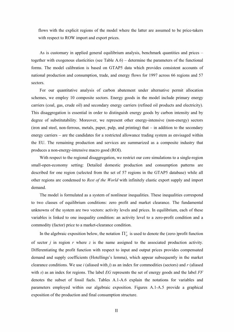
As is customary in applied general equilibrium analysis, benchmark quantities and prices –
together with exogenous elasticities (see Table A.6) – determine the parameters of the functional
forms. The model calibration is based on GTAP5 data which provides consistent accounts of
national production and consumption, trade, and energy flows for 1997 across 66 regions and 57
sectors.
For our quantitative analysis of carbon abatement under alternative permit allocation
schemes, we employ 10 composite sectors. Energy goods in the model include primary energy
carriers (coal, gas, crude oil) and secondary energy carriers (refined oil products and electricity).
This disaggregation is essential in order to distinguish energy goods by carbon intensity and by
degree of substitutability. Moreover, we represent other energy-intensive (non-energy) sectors
(iron and steel, non-ferrous, metals, paper, pulp, and printing) that – in addition to the secondary
energy carriers – are the candidates for a restricted allowance trading system as envisaged within
the EU. The remaining production and services are summarized as a composite industry that
produces a non-energy-intensive macro good (ROI).
With respect to the regional disaggregation, we restrict our core simulations to a single-region
small-open-economy setting: Detailed domestic production and consumption patterns are
described for one region (selected from the set of 57 regions in the GTAP5 database) while all
other regions are condensed to Rest of the World with infinitely elastic export supply and import
demand.
The model is formulated as a system of nonlinear inequalities. These inequalities correspond
to two classes of equilibrium conditions: zero profit and market clearance. The fundamental
unknowns of the system are two vectors: activity levels and prices. In equilibrium, each of these
variables is linked to one inequality condition: an activity level to a zero-profit condition and a
commodity (factor) price to a market-clearance condition.
In the algebraic exposition below, the notation zir� is used to denote the (zero-)profit function
of sector j in region r where z is the name assigned to the associated production activity.
Differentiating the profit function with respect to input and output prices provides compensated
demand and supply coefficients (Hotellings’s lemma), which appear subsequently in the market
clearance conditions. We use i (aliased with j) as an index for commodities (sectors) and r (aliased
with s) as an index for regions. The label EG represents the set of energy goods and the label FF
denotes the subset of fossil fuels. Tables A.1-A.6 explain the notations for variables and
parameters employed within our algebraic exposition. Figures A.1-A.5 provide a graphical
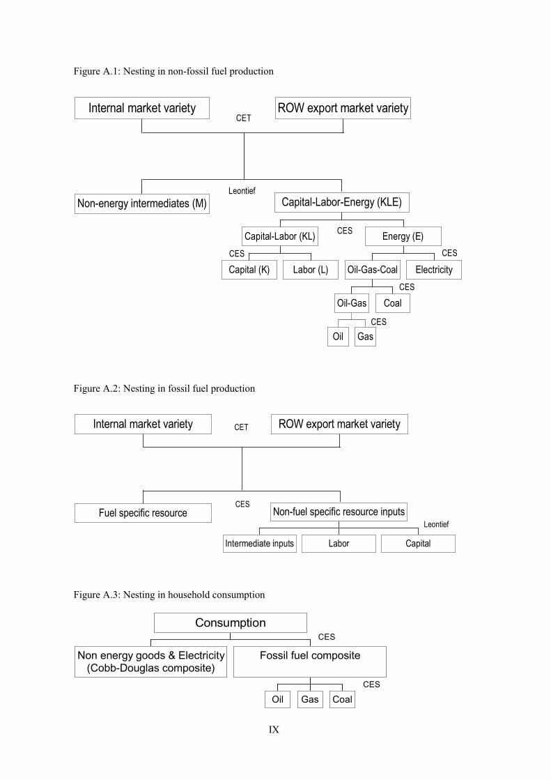
exposition of the production and final consumption structure.
III
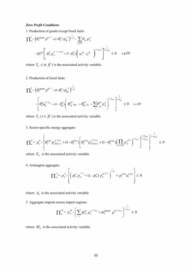
Zero Profit Conditions
1. Production of goods except fossil fuels:
� �
� �
1 11
1
1
(1 )
0 i FFKLE KLE
L KKLEjr jr
Y AXROW W Xir ir jir jrir
j EG
1- 1-1 -EE EKLE
ir ir ir rir r
= ir
+ ( )
p p p
1- p w v
� ��
� ��
� �
� � �
� � �
� �
�
�
� � �
� � �
��
� �� �
where irY ( i ff� ) is the associated activity variable.
2. Production of fossil fuels:
� �1 1
, ,
,
11
11 1
1
(1 )
(1 ) i FF0Q i Q i
Q i
Y XROW W Xir irir
Q Q FF FF FF Ar rir ir Lir Kir jrjir
j
= ir
ir
p p
q pw v
� ��
� �
�
�
� �
� � � �
� �
�
��
�
� �
� � � � � �
� �� �� � �� � � � ��
�
�
where irY ( i ff� ) is the associated activity variable.
3. Sector-specific energy aggregate:
� �111
11 11
{ , } { , }(1 ) (1 )
ELE ELECOA COAjirCOAELEE E ELE A ELE COA A COA A
ir ELE r ir ir COA r ir jririr j LQ = - p p p 0p
�� ��
��
�
� � � �
�
��
��
�
�
� �� �� �
� � � � � � � �� �
� �
��
where irE is the associated activity variable.
4. Armington aggregate:
� �1
11 2 2( ) 01
A1- -A AA A M CO COA A
ir ir r iir ir irir = - + p a p p p�
� �
� �
�� �� �� ��� �� ��
�
where irA is the associated activity variable.
5. Aggregate imports across import regions:1
0M
M M1-1-M 1-M M MROWX W
isr irir isirs
= - p p p�
� �
� �� �
� �� �� ���
where irM is the associated activity variable.
IV
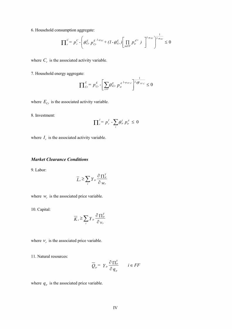
6. Household consumption aggregate:1
0EC ECirEC
1- 1-1-C C AEE ECr Cr irr Crr i FF
= - + (1- ) p p )p�
��
�
� ��
� �� � ��� � � � ��
where rC is the associated activity variable.
7. Household energy aggregate:
, ,
1
0FF C FF C
i FF
1- 1-E E AEiCrCr irCr = - p p � �
��
� � �� �� ���
where CrE is the associated activity variable.
8. Investment:0I I AI
ir irrri
= - pp � ���
where rI is the associated activity variable.
Market Clearance Conditions
9. Labor:Yir
irrri
YLw
� ��
��
where rw is the associated price variable.
10. Capital:Yir
irrri
YKv
� ��
��
where r� is the associated price variable.
11. Natural resources:
FFiq
Y = Qir
Yir
irir ��
��
where irq is the associated price variable.
V
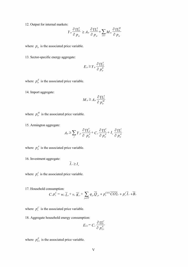
12. Output for internal markets:Y A Mir ir is
ir ir iss rir ir ir
Y A M p p p�
� � �� � ���
� � ��
where irp is the associated price variable.
13. Sector-specific energy aggregate:Yir
ir ir Eir
E Y p� �
��
where Eirp is the associated price variable.
14. Import aggregate:Air
ir ir Mir
M A p� �
��
where Mirp is the associated price variable.
15. Armington aggregate:Y C Ijr r r
ir jr r rA A Aj ir ir ir
+ + I CA Y p p p� � �� � �
�� � �
�
where Airp is the associated price variable.
16. Investment aggregate:r rI I�
where Irp is the associated price variable.
17. Household consumption:2 2C CO I
r rrr r rr jr r rjrr rj FF
p = + + q Q p CO p I BC w vL K�
� � ��
where Crp is the associated price variable.
18. Aggregate household energy consumption:
ECr
Cr
rCr p C = E
�
��
where ECrp is the associated price variable.
VI
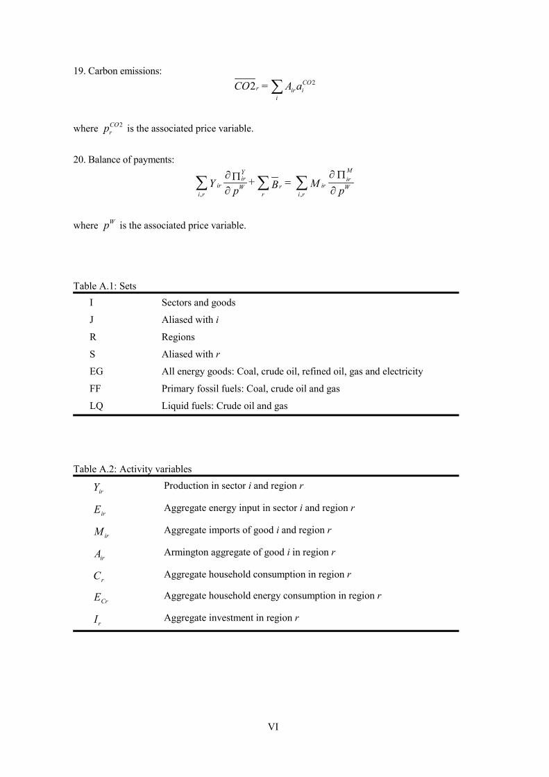
19. Carbon emissions:22 CO
ii
irr aA =CO �
where 2COrp is the associated price variable.
20. Balance of payments:
, ,
MYir ir
ir irrW Wi r r i r
+ Y MBp p� ���
�� �
� � �
where Wp is the associated price variable.
Table A.1: SetsI Sectors and goods
J Aliased with i
R Regions
S Aliased with r
EG All energy goods: Coal, crude oil, refined oil, gas and electricity
FF Primary fossil fuels: Coal, crude oil and gas
LQ Liquid fuels: Crude oil and gas
Table A.2: Activity variables
irY Production in sector i and region r
irE Aggregate energy input in sector i and region r
irM Aggregate imports of good i and region r
irA Armington aggregate of good i in region r
rC Aggregate household consumption in region r
CrE Aggregate household energy consumption in region r
rI Aggregate investment in region r
VII
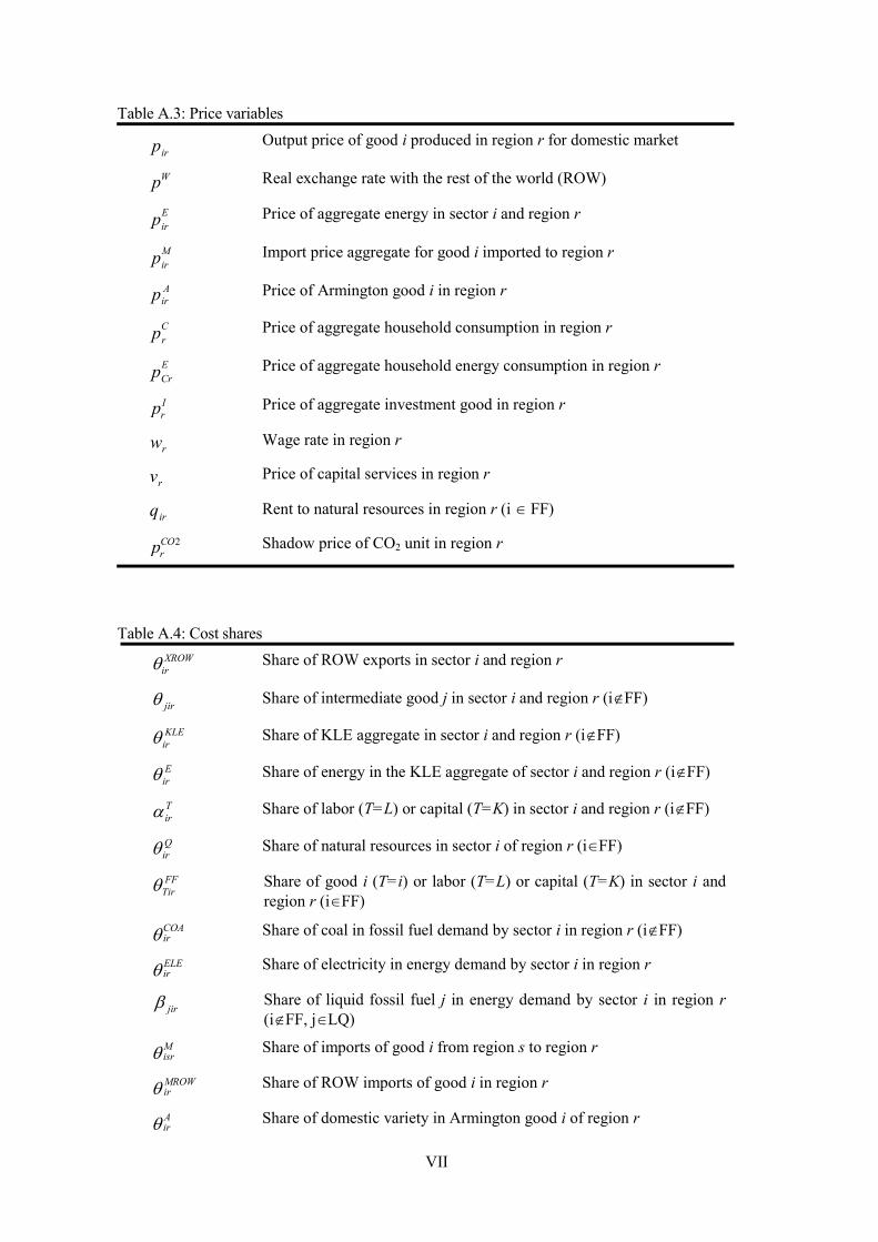
Table A.3: Price variables
pirOutput price of good i produced in region r for domestic market
Wp Real exchange rate with the rest of the world (ROW)
pEir
Price of aggregate energy in sector i and region r
pMir
Import price aggregate for good i imported to region r
Airp Price of Armington good i in region r
pCr
Price of aggregate household consumption in region r
pECr
Price of aggregate household energy consumption in region r
Irp Price of aggregate investment good in region r
rw Wage rate in region r
rv Price of capital services in region r
irq Rent to natural resources in region r (i � FF)
2COrp Shadow price of CO2 unit in region r
Table A.4: Cost sharesXROW
ir� Share of ROW exports in sector i and region r
jir� Share of intermediate good j in sector i and region r (i�FF)
KLEir� Share of KLE aggregate in sector i and region r (i�FF)
Eir� Share of energy in the KLE aggregate of sector i and region r (i�FF)
Tir� Share of labor (T=L) or capital (T=K) in sector i and region r (i�FF)
Qir� Share of natural resources in sector i of region r (i�FF)
FFTir� Share of good i (T=i) or labor (T=L) or capital (T=K) in sector i and
region r (i�FF)
�COAir Share of coal in fossil fuel demand by sector i in region r (i�FF)
�ELEir
Share of electricity in energy demand by sector i in region r
jir� Share of liquid fossil fuel j in energy demand by sector i in region r(i�FF, j�LQ)
�Misr
Share of imports of good i from region s to region r
MROWir� Share of ROW imports of good i in region r
�Air
Share of domestic variety in Armington good i of region r
VIII
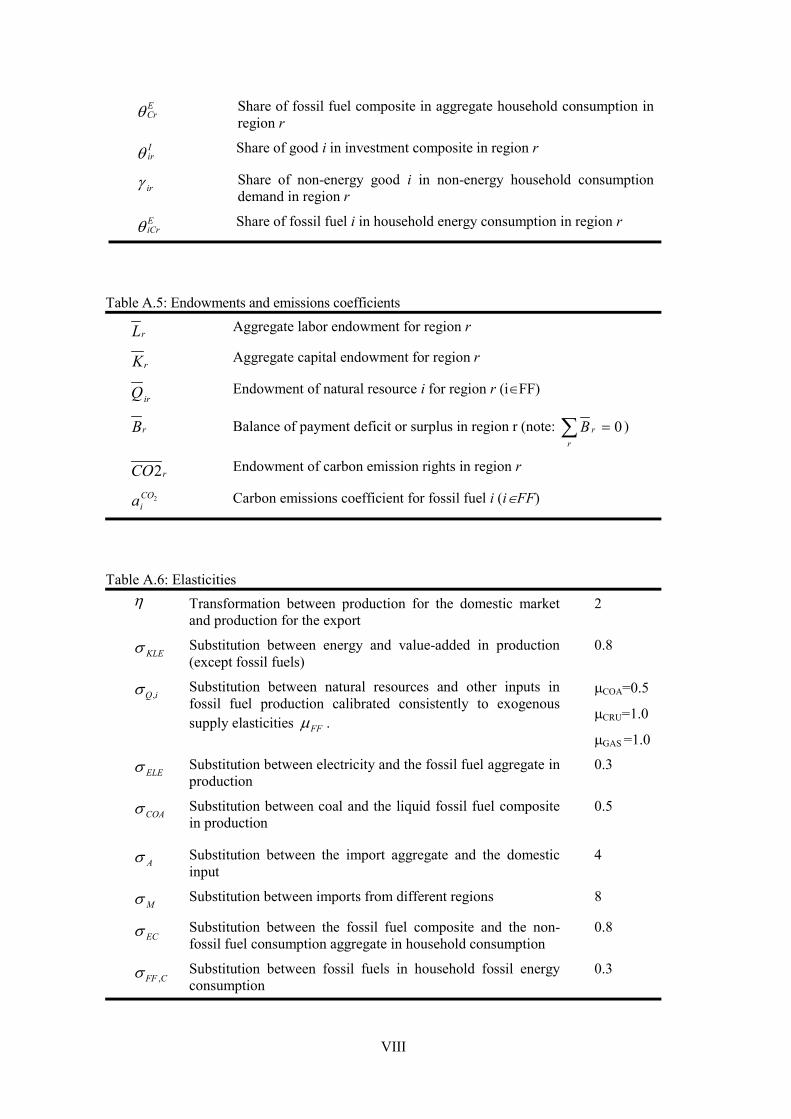
�ECr
Share of fossil fuel composite in aggregate household consumption inregion r
Iir�
Share of good i in investment composite in region r
ir� Share of non-energy good i in non-energy household consumptiondemand in region r
�EiCr
Share of fossil fuel i in household energy consumption in region r
Table A.5: Endowments and emissions coefficients
Lr Aggregate labor endowment for region r
rK Aggregate capital endowment for region r
irQ Endowment of natural resource i for region r (i�FF)
Br Balance of payment deficit or surplus in region r (note: 0��r
rB )
2rCO Endowment of carbon emission rights in region r
2COia Carbon emissions coefficient for fossil fuel i (i�FF)
Table A.6: Elasticities� Transformation between production for the domestic market
and production for the export2
KLE� Substitution between energy and value-added in production(except fossil fuels)
0.8
iQ,� Substitution between natural resources and other inputs infossil fuel production calibrated consistently to exogenoussupply elasticities FF� .
�COA=0.5
�CRU=1.0
�GAS =1.0
ELE� Substitution between electricity and the fossil fuel aggregate inproduction
0.3
COA� Substitution between coal and the liquid fossil fuel compositein production
0.5
A� Substitution between the import aggregate and the domesticinput
4
M� Substitution between imports from different regions 8
EC�Substitution between the fossil fuel composite and the non-fossil fuel consumption aggregate in household consumption
0.8
,FF C�Substitution between fossil fuels in household fossil energyconsumption
0.3
IX
Figure A.1: Nesting in non-fossil fuel production
CES
CESCES
CES
CET
CES
Leontief
CES
Internal market variety ROW export market variety
Non-energy intermediates (M)
Capital (K) Labor (L)
Capital-Labor (KL)
Oil Gas
Oil-Gas Coal
Oil-Gas-Coal Electricity
Energy (E)
Capital-Labor-Energy (KLE)
Figure A.2: Nesting in fossil fuel production
CES
Leontief
CETInternal market variety ROW export market variety
Fuel specific resource
Intermediate inputs Labor Capital
Non-fuel specific resource inputs
Figure A.3: Nesting in household consumption
CES
CES
Non energy goods & Electricity(Cobb-Douglas composite)
Oil Gas Coal
Fossil fuel composite
Consumption

X
Figure A.4: Nesting in Armington production
CES
Internal market variety Import aggregate
Armington good
Figure A.5: Nesting in import aggregate
CES
Region 1 Region 2 ...
Import varieties from other explicit regions
ROW import market variety
Import aggregate
Implementation of Allowance Allocation Rules
In our simulations on alternative allowance allocation rules, the price of a unit of CO2 for an
industry i or the household C depends on whether the respective segment of the economy is
eligible for carbon trade (denoted T ). To distinguish carbon prices by sector, we must explicitly
account for carbon demands within the zero-profit conditions characterizing the sector-specific
energy aggregate and the household energy aggregate (instead of the Armington aggregate).
Carbon demands by segments i or C then reads as:
2 22( )
Eir
ir ir CO COj ff jr j jr
CO = E p a p
�
� �
� �� and 2 22
( )
Cr
Cr Cr CO COj ff jr j jr
CO = E p a p
�
� �
� �� .
Allowances can be traded internationally at an exogenous world market price. In the algebraic
formulation, two additional zero profit conditions must be added to specify carbon import
activities 2COzrIM and carbon export activities 2CO
zrEX for segments z of the economy that are open
to international trade ( z T� ):
2W COzrep p� (imports) and 2CO W
zrp ep� (exports)
where W ep denotes the international price for a unit of CO2 in domestic currency. Revenues from
exports of emission allowances or, likewise, expenditures for imports of carbon emission rights
enter the balance of payment constraints. The market clearance condition for those segments that
form part of allowance trading reads as:
XI
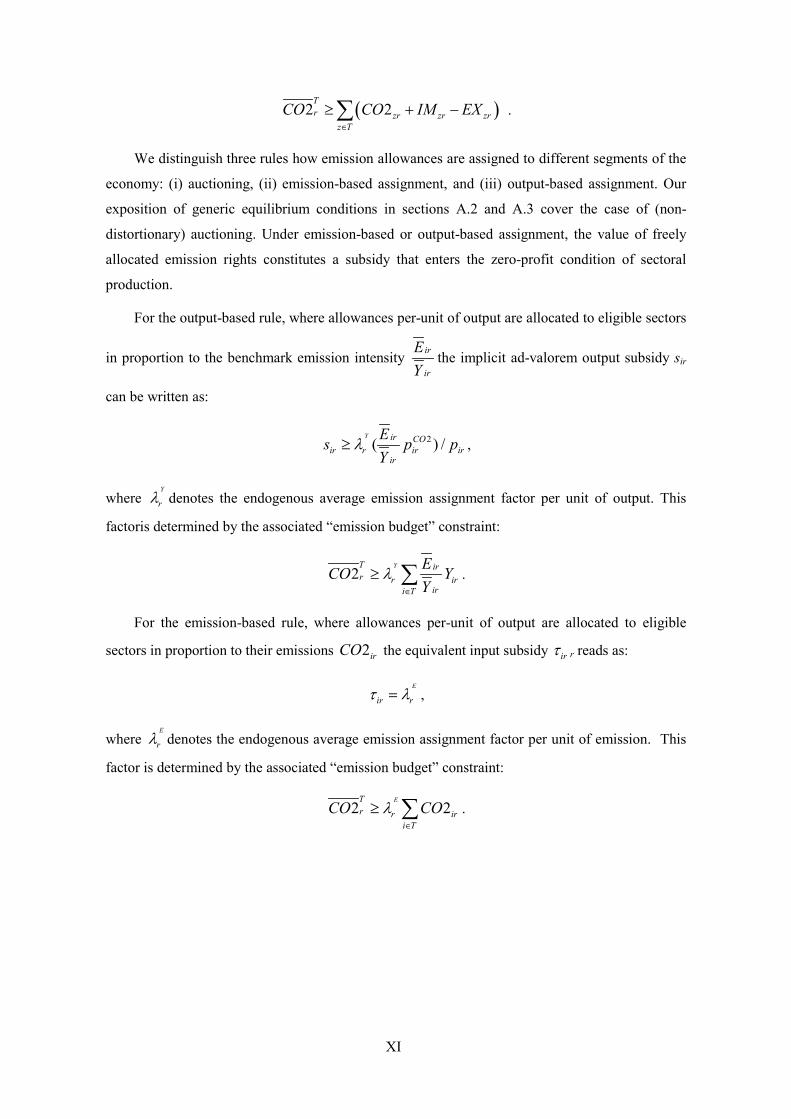
� �2 2Tr zr zr zr
z TCO CO IM EX
�
� � �� .
We distinguish three rules how emission allowances are assigned to different segments of the
economy: (i) auctioning, (ii) emission-based assignment, and (iii) output-based assignment. Our
exposition of generic equilibrium conditions in sections A.2 and A.3 cover the case of (non-
distortionary) auctioning. Under emission-based or output-based assignment, the value of freely
allocated emission rights constitutes a subsidy that enters the zero-profit condition of sectoral
production.
For the output-based rule, where allowances per-unit of output are allocated to eligible sectors
in proportion to the benchmark emission intensity ir
ir
EY
the implicit ad-valorem output subsidy sir
can be written as:
2( ) /Y ir CO
ir r ir irir
Es p pY
�� ,
where Y
r� denotes the endogenous average emission assignment factor per unit of output. This
factoris determined by the associated “emission budget” constraint:
2YT ir
r r iriri T
ECO YY
�
�
� � .
For the emission-based rule, where allowances per-unit of output are allocated to eligible
sectors in proportion to their emissions 2irCO the equivalent input subsidy ir� r reads as:
E
ir r� �� ,
where E
r� denotes the endogenous average emission assignment factor per unit of emission. This
factor is determined by the associated “emission budget” constraint:
2 2ET
r r iri T
CO CO�
�
� � .
XII
Appendix B: Sensitivity Analysis
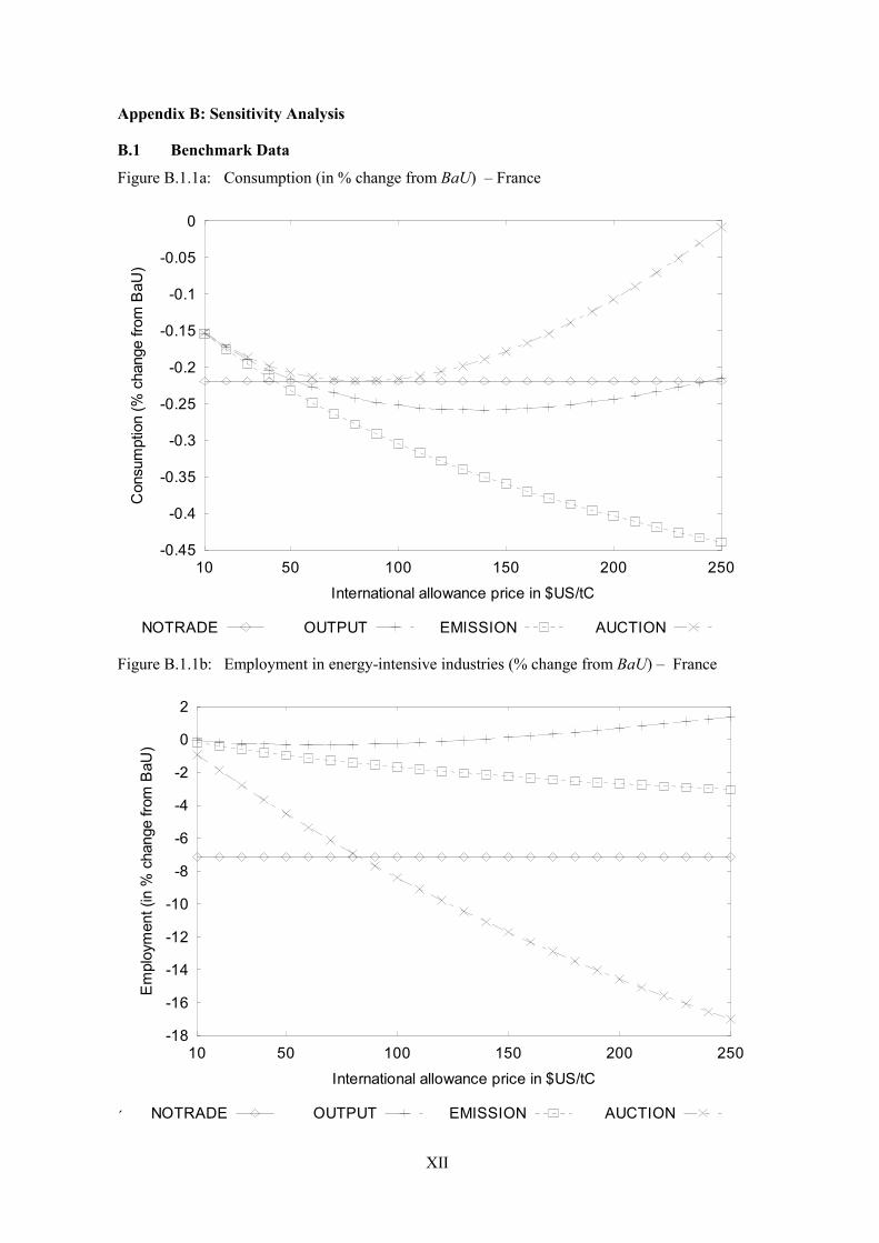
B.1 Benchmark Data
Figure B.1.1a: Consumption (in % change from BaU) – France
-0.45
-0.4
-0.35
-0.3
-0.25
-0.2
-0.15
-0.1
-0.05
0
10 50 100 150 200 250
Con
sum
ptio
n (%
cha
nge
from
BaU
)
International allowance price in $US/tC
NOTRADE OUTPUT EMISSION AUCTION
Figure B.1.1b: Employment in energy-intensive industries (% change from BaU) – France
´
-18
-16
-14
-12
-10
-8
-6
-4
-2
0
2
10 50 100 150 200 250
Em
ploy
men
t (in
% c
hang
e fro
m B
aU)
International allowance price in $US/tC
NOTRADE OUTPUT EMISSION AUCTION
XIII
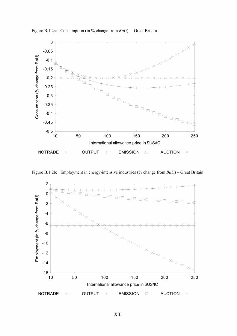
Figure B.1.2a: Consumption (in % change from BaU) – Great Britain
-0.5
-0.45
-0.4
-0.35
-0.3
-0.25
-0.2
-0.15
-0.1
-0.05
0
10 50 100 150 200 250
Con
sum
ptio
n (%
cha
nge
from
BaU
)
International allowance price in $US/tC
NOTRADE OUTPUT EMISSION AUCTION
Figure B.1.2b: Employment in energy-intensive industries (% change from BaU) – Great Britain
-16
-14
-12
-10
-8
-6
-4
-2
0
2
10 50 100 150 200 250
Em
ploy
men
t (in
% c
hang
e fro
m B
aU)
International allowance price in $US/tC
NOTRADE OUTPUT EMISSION AUCTION
XIV
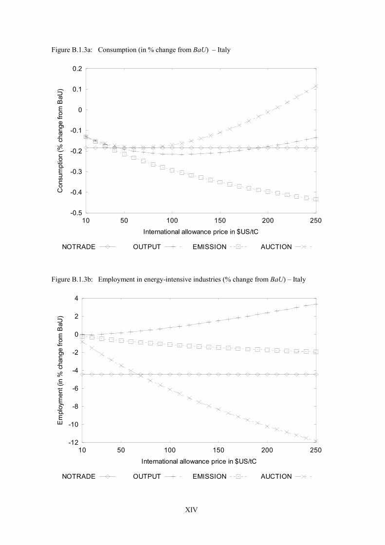
Figure B.1.3a: Consumption (in % change from BaU) – Italy
-0.5
-0.4
-0.3
-0.2
-0.1
0
0.1
0.2
10 50 100 150 200 250
Con
sum
ptio
n (%
cha
nge
from
BaU
)
International allowance price in $US/tC
NOTRADE OUTPUT EMISSION AUCTION
Figure B.1.3b: Employment in energy-intensive industries (% change from BaU) – Italy
-12
-10
-8
-6
-4
-2
0
2
4
10 50 100 150 200 250
Em
ploy
men
t (in
% c
hang
e fro
m B
aU)
International allowance price in $US/tC
NOTRADE OUTPUT EMISSION AUCTION
XV
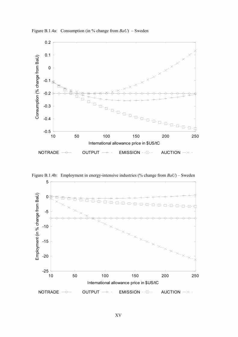
Figure B.1.4a: Consumption (in % change from BaU) – Sweden
-0.5
-0.4
-0.3
-0.2
-0.1
0
0.1
0.2
10 50 100 150 200 250
Con
sum
ptio
n (%
cha
nge
from
BaU
)
International allowance price in $US/tC
NOTRADE OUTPUT EMISSION AUCTION
Figure B.1.4b: Employment in energy-intensive industries (% change from BaU) – Sweden
-25
-20
-15
-10
-5
0
5
10 50 100 150 200 250
Em
ploy
men
t (in
% c
hang
e fro
m B
aU)
International allowance price in $US/tC
NOTRADE OUTPUT EMISSION AUCTION
XVI
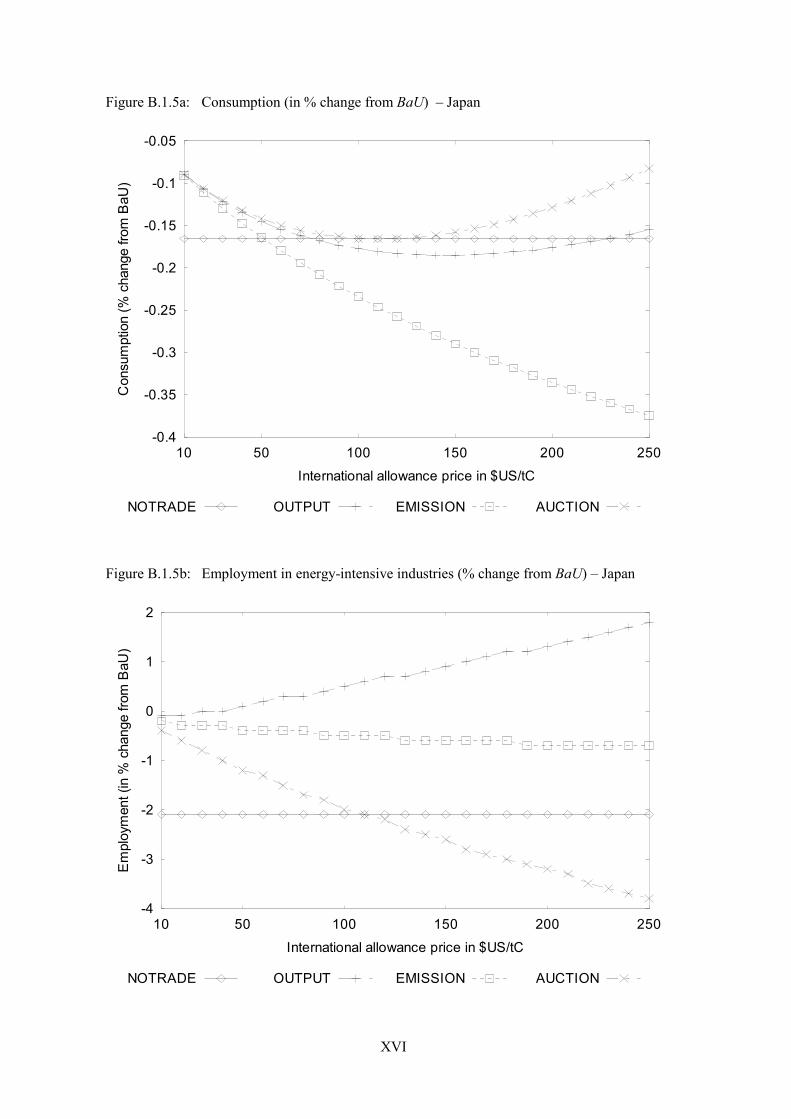
Figure B.1.5a: Consumption (in % change from BaU) – Japan
-0.4
-0.35
-0.3
-0.25
-0.2
-0.15
-0.1
-0.05
10 50 100 150 200 250
Con
sum
ptio
n (%
cha
nge
from
BaU
)
International allowance price in $US/tC
NOTRADE OUTPUT EMISSION AUCTION
Figure B.1.5b: Employment in energy-intensive industries (% change from BaU) – Japan
-4
-3
-2
-1
0
1
2
10 50 100 150 200 250
Em
ploy
men
t (in
% c
hang
e fro
m B
aU)
International allowance price in $US/tC
NOTRADE OUTPUT EMISSION AUCTION
XVII
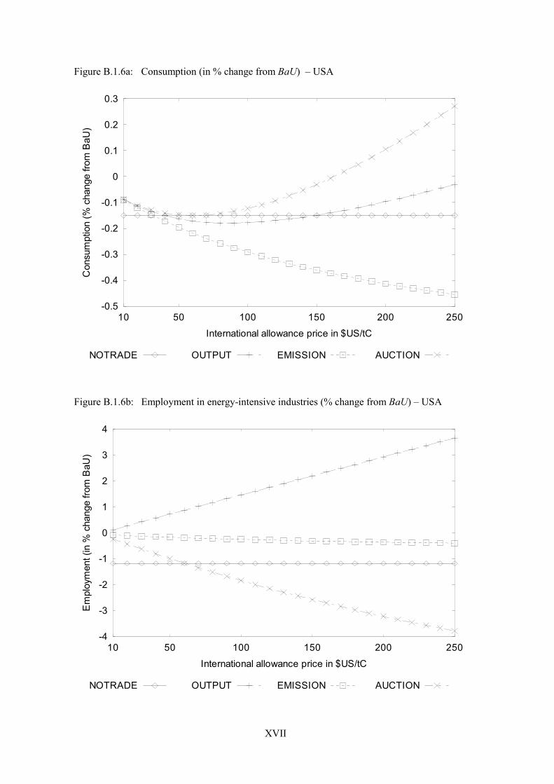
Figure B.1.6a: Consumption (in % change from BaU) – USA
-0.5
-0.4
-0.3
-0.2
-0.1
0
0.1
0.2
0.3
10 50 100 150 200 250
Con
sum
ptio
n (%
cha
nge
from
BaU
)
International allowance price in $US/tC
NOTRADE OUTPUT EMISSION AUCTION
Figure B.1.6b: Employment in energy-intensive industries (% change from BaU) – USA
-4
-3
-2
-1
0
1
2
3
4
10 50 100 150 200 250
Em
ploy
men
t (in
% c
hang
e fro
m B
aU)
International allowance price in $US/tC
NOTRADE OUTPUT EMISSION AUCTION
XVIII
B.2 Reduction Targets
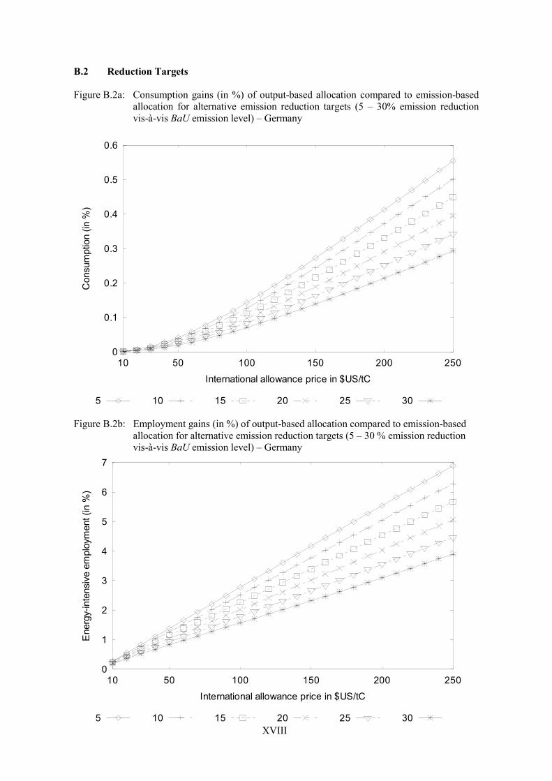
Figure B.2a: Consumption gains (in %) of output-based allocation compared to emission-basedallocation for alternative emission reduction targets (5 – 30% emission reductionvis-à-vis BaU emission level) – Germany
0
0.1
0.2
0.3
0.4
0.5
0.6
10 50 100 150 200 250
Con
sum
ptio
n (in
%)
International allowance price in $US/tC
5 10 15 20 25 30
Figure B.2b: Employment gains (in %) of output-based allocation compared to emission-basedallocation for alternative emission reduction targets (5 – 30 % emission reductionvis-à-vis BaU emission level) – Germany
0
1
2
3
4
5
6
7
10 50 100 150 200 250
Ene
rgy-
inte
nsiv
e em
ploy
men
t (in
%)
International allowance price in $US/tC
5 10 15 20 25 30
XIX
B.3 Multilateral Abatement
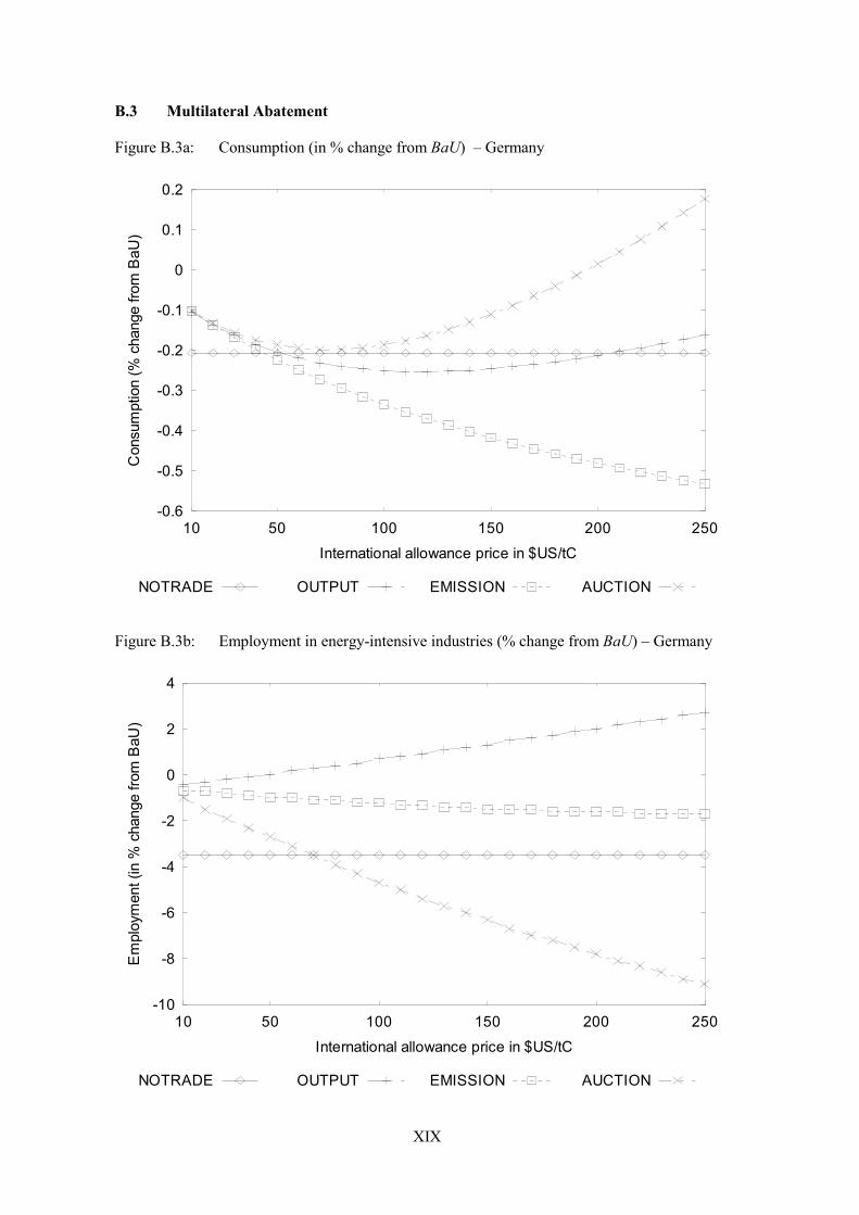
Figure B.3a: Consumption (in % change from BaU) – Germany
-0.6
-0.5
-0.4
-0.3
-0.2
-0.1
0
0.1
0.2
10 50 100 150 200 250
Con
sum
ptio
n (%
cha
nge
from
BaU
)
International allowance price in $US/tC
NOTRADE OUTPUT EMISSION AUCTION
Figure B.3b: Employment in energy-intensive industries (% change from BaU) – Germany
-10
-8
-6
-4
-2
0
2
4
10 50 100 150 200 250
Em
ploy
men
t (in
% c
hang
e fro
m B
aU)
International allowance price in $US/tC
NOTRADE OUTPUT EMISSION AUCTION

XX
B.4 Market Structure (Cournot Competition in Energy-intensive Industries)
Figure B.4a: Consumption (in % change from BaU) – Germany
-0.7
-0.6
-0.5
-0.4
-0.3
-0.2
-0.1
0
0.1
10 50 100 150 200 250
Con
sum
ptio
n (%
cha
nge
from
BaU
)
International allowance price in $US/tC
NOTRADE OUTPUT EMISSION AUCTION
Figure B.4b: Employment in energy-intensive industries (% change from BaU) – Germany
-30
-25
-20
-15
-10
-5
0
5
10 50 100 150 200 250
Em
ploy
men
t (in
% c
hang
e fro
m B
aU)
International allowance price in $US/tC
NOTRADE OUTPUT EMISSION AUCTION