Economic multiple model predictive control for HVAC

Economic multiple model predictive control for HVAC systems - A 1

case study for a food manufacturer in Germany 2

3

Tobias Heidrich a, Jonathan Grobe a, Henning Meschede a, Jens Hesselbach a 4 a Department for Sustainable Products and Processes (upp), University of Kassel, Kassel, 34125, Germany 5 [email protected] 6

7

Keywords: Model Predictive Control, HVAC, Climate control, Flexible Control Technologies 8

9

A B S T R A C T 10

The following paper describes an economical, multiple model predictive control (EMMPC) for an air 11 conditioning system of a confectionery manufacturer in Germany. The application consists of a 12 packaging hall for chocolate bars, in which a new local conveyor belt air conditioning system is used 13 and thus the temperature and humidity limits in the hall can be significantly extended. The EMMPC 14 calculates the optimum energy or cost humidity and temperature set points in the hall. For this purpose, 15 time-discrete state space models and an economic objective function with which it is possible to react 16 to flexible electricity prices in a cost-optimised manner are created. A possible future electricity price 17 model for Germany with a flexible EEG levy was used as a flexible electricity price. The flexibility 18 potential is determined by variable temperature and humidity limits in the hall, which are oriented 19 towards the comfort field for easily working persons, and the building mass. The building mass of the 20 created room model is used as a thermal energy store. Considering electricity price and weather 21 forecasts as well as internal, production plan-dependent load forecasts, the model predictive controller 22 directly controls the heating and cooling register and the humidifier of the air conditioning system. 23

24

1. Introduction and problem description 25

A constantly increasing scarcity of resources, increasing emissions and the global warming proven in 26 many scientific studies require differentiated and comprehensive solutions [1] [2] [3]. In addition to a 27 more efficient use of resources, the conversion of the energy supply system to an increased use of 28 renewable energies is also decisive for achieving these goals, which in turn leads to an increase in 29 balancing fluctuating residual loads in the electricity grid. With regard to the global energy demand it 30 can be seen that about one third s caused in the building sector [4], of which about half of the energy 31 demand is accounted for by building heating, ventilation and air conditioning (HVAC) [5] [6]. In view 32 of these circumstances, energy efficiency measures and the use of more flexible energy supply 33 technologies in the building sector and in the field of building air conditioning are substantial solutions 34 to the challenges described. 35

In the field of building HVAC, high energy saving potentials can be exploited in many ways. Scientific 36 research focuses on different air routing concepts, the further development of the various components 37 of an air conditioning system and, above all, the improvement of control technology [7] [8] [9]. Due to 38 the volatile nature of wind and solar energy demand has to be made more flexible. Hence, energy 39 demand can be adopted to energy supply and therefor stabilise the energy system through demand 40 response on the one hand and increase the utilisation rate of renewable energy systems on the other 41 hand [10] [11]. 42

Preprints (www.preprints.org) | NOT PEER-REVIEWED | Posted: 7 November 2018 doi:10.20944/preprints201811.0146.v1

© 2018 by the author(s). Distributed under a Creative Commons CC BY license.

Peer-reviewed version available at Energies 2018, 11, 3461; doi:10.3390/en11123461

http://dx.doi.org/10.20944/preprints201811.0146.v1

http://creativecommons.org/licenses/by/4.0/

http://dx.doi.org/10.3390/en11123461

By developing and implementing an economical, multiple, model predictive control (EMMPC), this 43 flexibility potential can be realised in an energy- or cost-optimised manner. Demand response can be 44 fulfilled by integrating future, flexible electricity price models based on electricity supply and demand. 45 For the flexible operation of the air conditioning the air mass of any hall is used as thermal energy 46 storage. Hence, allowing a range of temperature and humidity specifications is key requirement [12] 47 [13] [14]. Especially in industries, these ranges are often not given due to fixed settings and strict 48 specifications of the product. Flexible and efficient control of full air conditioning systems requires the 49 solution of complex tasks. Time-varying internal and external disturbances affect the controlled system, 50 many processes involve time delays, the system goes through many operating conditions, and the 51 required energy can also have variable price structures. An efficient control approach should therefore 52 be able to take into account time-dependent disturbances, map a wide range of operating conditions and 53 process variable price structures. 54

With regard to the current state of research, this paper applies an advanced EMMPC approach for the 55 flexible operation of air conditioning systems in industrial productions. Hereby, the EMMPC approach 56 combines both, the approach of multiple and economic MPC to control and optimise non-linear systems 57 under several constraints. The realisation of the flexible air conditioning is shown for a real case of a 58 packaging hall for chocolate bars. The product has strict temperature and humidity specifications. 59 Therefore, the implementation of a new, local conveyor belt air conditioning system is indispensable to 60 soften up these specifications for the hall [12] [15][14]. 61

62

2. State of research 63

Due to the manifold tasks that an air conditioning system has to fulfil, the system control is highly 64 complex. Depending on the design and application, the air temperature, humidity, air volume flow and 65 air mixtures (fresh air/exhaust air ratio) must be adjusted and controlled. Since these variables influence 66 each other, the degree of complexity increases significantly. For these reasons, a combination of 67 different control approaches and sequence circuits, which control the respective sub-components and 68 bring them into a meaningful connection, is often necessary to ensure efficient plant operation. In the 69 field of efficient and flexible building air conditioning, a large number of scientific studies can be 70 considered. 71

The publication of Afram and Janabi-Sharifi (2014) [16] gives a good overview of control approaches 72 used or under development for air conditioning systems. A distinction is made between "classic 73 control", "hard control", "soft control", and "hybrid control" for air conditioning systems as well as 74 further approaches that cannot be assigned to these categories. The classic control corresponds to the 75 state of the art and are widely and practically applied. The classic control methods for HVAC systems 76 include two-point controllers (on/off), proportional (P), proportional integral (PI), and proportional 77 integral differential (PID) controllers. The so-called "hard control" for air conditioning systems include 78 gain scheduling, optimum control, robust control, model predictive control (MPC) and nonlinear and 79 adaptive control. MPC, as described in this publication, use previously created models of the system to 80 be controlled to predict and optimise future system behaviour under changing boundary conditions. 81 Such controllers can be used both as a replacement for classic controllers and can also perform higher-82 level control tasks. 83

So-called fuzzy controllers or the use of artificial neural networks are summarised under the term "soft" 84 or "soft control". These comparatively new methods for controlling HVAC systems can replace both 85 higher-level and local controllers and perform a wide range of tasks. Fuzzy controllers are based on if-86 then-else instructions and require a sufficiently deep understanding of the system to be controlled. 87




http://dx.doi.org/10.3390/en11123461

Artificial neural networks, on the other hand, are trained with data, the understanding of the system is 88 irrelevant [17]. Ruano et al. (2016), for example, investigated a predictive control in which a neural 89 network predicts building and system behaviour and is optimised by including weather forecasts [18]. 90 "Hybrid control techniques" deal with a combination of soft and hard control approaches [17]. 91

Furthermore, the hierarchical arrangement of different controllers is also subject of some research. For 92 example, MPC controllers can be used as so-called "super visory control", which in turn transmit higher-93 level setpoints to underlying control structures - this can also be another MPC controller [19] [20]. 94

Publications dealing exclusively with the comparison of control methods for air conditioning systems 95 and providing a comprehensive overview of the state of research favour the use of MPC to solve the 96 challenges of flexible operation mentioned above [16] [21]. In both studies, the authors summarise that 97 classical regulatory approaches are primarily suitable for less complex regulatory tasks. Outside the 98 previously defined operating point, classic controllers often work too slowly or react too aggressively, 99 for example. The soft methods require either a very extensive understanding of the system to be 100 controlled or comprehensive measured value analyses. In addition, the acceptance of so-called "black-101 box" approaches, such as the soft approaches, is not widespread in industry; an introduction is usually 102 very lengthy and impractical due to too little data. In opposite to that, hard methods like MPC require a 103 complex and rigorous mathematical investigation of the system. The identification of linear subareas in 104 the system behaviour, which is necessary for control using hard control techniques over non-linear 105 operating ranges, often proves to be difficult and very complex. Nevertheless, the authors emphasize 106 that the model predictive approach as a hard control technology is particularly well suited for complex 107 control tasks in the field of air conditioning due to its capabilities and can fulfil the aforementioned 108 tasks. 109

The many advantages are offset above all by the high and complex programming effort. A sufficiently 110 precise understanding of the system is just as necessary as correspondingly modern hardware and 111 software. The use of MPC controllers is primarily based on linear process models [16] while its 112 definition is very challenging and not standardised. Especially for multi-variable systems with many 113 non-linearities in system behaviour, as they often occur in building air conditioning and increase 114 significantly due to the increasing complexity of an air conditioning system. However, the integration 115 of so-called multiple MPC controllers or adaptive MPC control structures offers great prospects of 116 success in controlling non-linear controlled systems in an optimised manner [22] [23].This is where the 117 publication comes in and is intended to contribute to the implementation and realisation of an EMMPC 118 for HVAC systems. 119

120

3. Methodology and fundamentals of the used model predictive control 121

The developed, model-predictive control uses a linear, time-invariant (LTI) and time-discrete prediction 122 model of the system to be controlled (time-discrete state space models of an air conditioning system 123 with a connected building) to calculate future state and output changes over a finite prediction horizon. 124 The aim is to minimise the set point deviation (fixed controlled variable, energy or costs) over the 125 prediction horizon. 126

In order to determine the best possible control variable sequence for minimising the target function 127 within a prediction horizon, an optimisation problem is solved. The prediction horizon describes the 128 entire period under which the optimisation takes place. Up to a pre-determinable time step, optimised 129 control signals of the MPC controller and adapted predicted boundary conditions are considered. The 130 number of time steps over which predicted, optimised control signals are calculated is defined by 131




http://dx.doi.org/10.3390/en11123461

defining the control horizon. The control horizon is at most as long as the prediction horizon, which 132 usually corresponds to half of the prediction horizon based on the calculation duration. At the end of 133 the control horizon, the last control signal is kept constant until the end of the prediction horizon. [22] 134 [23] 135

Individually defined limitations of output and control variables are included in the optimisation problem 136 via slack variables. The first optimum control variable value is used for controlling the system. The 137 measured actual values as well as current control and disturbance variables are used for the subsequent 138 time step for the new calculation of the optimum control variable sequence. 139

The system to be controlled consists of physical models of a building and a HVAC system, which are 140 described in more detail in section 4. From these physical models linear, time-discrete state space 141 models are derived, which function as prediction models as part of the MPC as shown in figure 1. Using 142 the optimisation algorithm, optimised control signals adapted to the boundary conditions are transmitted 143 to the system to be controlled. The MPC directly controls the heating and cooling coil as well as the 144 humidifier with control signals (manipulated variables). The control signals are limited between 0 and 145 1. The fans are not controlled via MPC and are operated with a constant volumetric flow of 2000 m³/h. 146 The condition of the supply air is composed of fresh air conditions and the respective conditioning of 147 the climate functions controlled via the control variables. The temperature and humidity of the indoor 148 air is calculated from the proportion of indoor air, supply air and outdoor temperature. 149

A schematic overview of the structure and functionality of the MPC is given in the following figure 150 (fig. 1). 151

Figure 1: Schematic structure of the model predictive control system 152

153

Air cooling in the model can be realised with two processes: either a dehumidification process 154 (condensate formation) or dry cooling (without condensate formation) is applied. This behaviour cannot 155 be represented in one linear system, since a latent phase transition occurs after reaching the saturation 156 temperature. Consequently, for both cases a multiple model predictive controller with two different 157 prediction models is used in the following. If condensate formation occurs, the prediction model A is 158 switched over to the prediction model B. The two prediction models are based on a multiple model 159 predictive controller. The two prediction models are generated around different operating points (with 160 and without condensation) by linearizing the whole model. Due to the thermal inertia of the system, a 161 time step of 900 s is applied. 162

Optimiser

Manipulated Variables: Heater Humidifier Cooler

Electricity Price Outputs: Temperature Absolute humidity Actual Power

Measured Disturbances: Ambient temperature Ambient absolute humidity Thermal load Humidity input

MPC

Prediction Model

Room HVAC

System




http://dx.doi.org/10.3390/en11123461

163

3.1 Time Discrete State Space Model 164

The developed MPC uses, as described before, time-discrete LTI systems instead of time-continuous 165 systems. Hence, the equation of state does not describe the derivative x(t) of the states, but the states of 166 discrete, future sampling times x(k+1). The matrices AD (state matrix) and BD (input matrix) of the time-167 discrete state space representation result from the general solution of the temporal course of the state 168 variable x from time t0. 169

Accordingly, the matrices AD and BD are formed at the sampling times T. The sampling time is the 170 duration of a time step in the discrete system. The matrices C (output matrix) and D (feedthrough 171 matrix) remain unchanged in comparison to the time continuous system [24] [25]: 172

The time-discrete representation used is as follows: 173

input equation: x(k + 1) = A x(k) + B u(k)

output equation: y(k) = Cx(k) + Du(k) (1)

174

3.2 Optimisation problem and solution methods 175

The core of the developed MPC is an optimisation algorithm for calculating the optimal control variable 176 sequence z : 177

z = [u(k|k) u(k + 1|k) . . .u(k + p − 1|k) ε ] (2)

The deviations of the actual values from the target values of the controlled system are minimised over 178 the prediction horizon, taking restrictions into account. The objective function J(z ) consists of four 179 parts: 180

J(z ) = J (z ) + J (z ) + J∆ (z ) + J (z ) (3)

Output Reference Tracking: 181

J (z ) = w ,

s r (k + i|k) − y (k + i|k)

(4)

Manipulated Variable Tracking: 182

J (z ) = w ,

s u (k + i|k) − u , (k + i|k)

(5)

Manipulated Variable Move Suppression: 183




http://dx.doi.org/10.3390/en11123461

J∆ (z ) = w ,∆

s u (k + i|k) − u (k + i − 1|k)

(6)

Constraint Violation: 184

J (z ) = ρ ϵ (7)

The output variables y(k) can be described with the internal prediction model, the current states x(k) 185 and inputs u(k). From this it follows that the objective functionJ(z ) depends only on the decision 186 variable z . [23] 187

In each step of a sequence {x } , an approximate quadratic subproblem is formed from the first and 188 second derivatives of the objective function at point x . 189

By defining weights and scales, the aggressiveness of the control signals can be adjusted by defining 190 the suppression of changes. 191

The described objective function is minimised by the method of sequential quadratic programming 192 (SQP) which is an extension of quadratic programming (QP) and one of the most effective methods for 193 solving nonlinear, nonlinear-restricted optimisation problems [26]. 194

195

3.3 Multiple Model Predictive Control 196

In order to keep the deviations between a linear model for control and the real system small over a larger 197 working range, there is the possibility of multiple model predictive control (MMPC). With the MMPC, 198 several controllers with different internal models and parameters are combined in a block and selected 199 via an additional input ("switch"). Depending on the environmental and operating conditions, the most 200 suitable time-discrete state space model can be selected to calculate the optimum control variable 201 sequence for the system. 202

203

3.4 Economic Model Predictive Control 204

The aim of the economic, model-predictive regulation is to minimise monetary costs. The objective 205 function is formulated in such a way that the current and predicted electricity price multiplied by the 206 current and predicted output over the prediction horizon p is minimised. The suppression of changes in 207 the control variables ∑ ∑ (du ∙ W ) and the minimisation of restriction violations W ∙ ϵ 208 remain the same in comparison to set point compliance or energy optimisation. 209

J (z ) = (P ∙ k ) +

(∆u ∙ W∆ ) + W ∙ ϵ

(8)

The room temperature and absolute humidity of the room air are kept above restrictions in the comfort 210 field. 211

212

4. Model description 213




http://dx.doi.org/10.3390/en11123461

In this section, the analysed system based on a real confectionery manufacturer and the models used to 214 calculate flexibility and savings potentials are described. The system consists of a packaging hall for 215 chocolate bars, which are cooled by a novel, local air-conditioning system introduced by Heidrich et al. 216 [12] and a connected air-conditioning system for providing conditioned are to the rest of the hall within 217 the limits of the comfort field for workers. 218

Without local air-conditioning of the chocolate bars, the entire hall would have to be air-conditioned to 219 18°C and 50 % relative humidity in order to avoid deformation of the chocolate, which begins to melt 220 at 18°C, condensation effects on the chocolate bar, which is cooled from the aisle to the conveyor belt 221 at around 14-15°C, and problems with electrostatic charging of the packaging cardboard [14] [27] [28]. 222

In the hall, there are also packaging machines and medium-heavy working staff emitting heat and water. 223 The number of staff depends on the shift (production in operation, no production, cleaning shift). 224

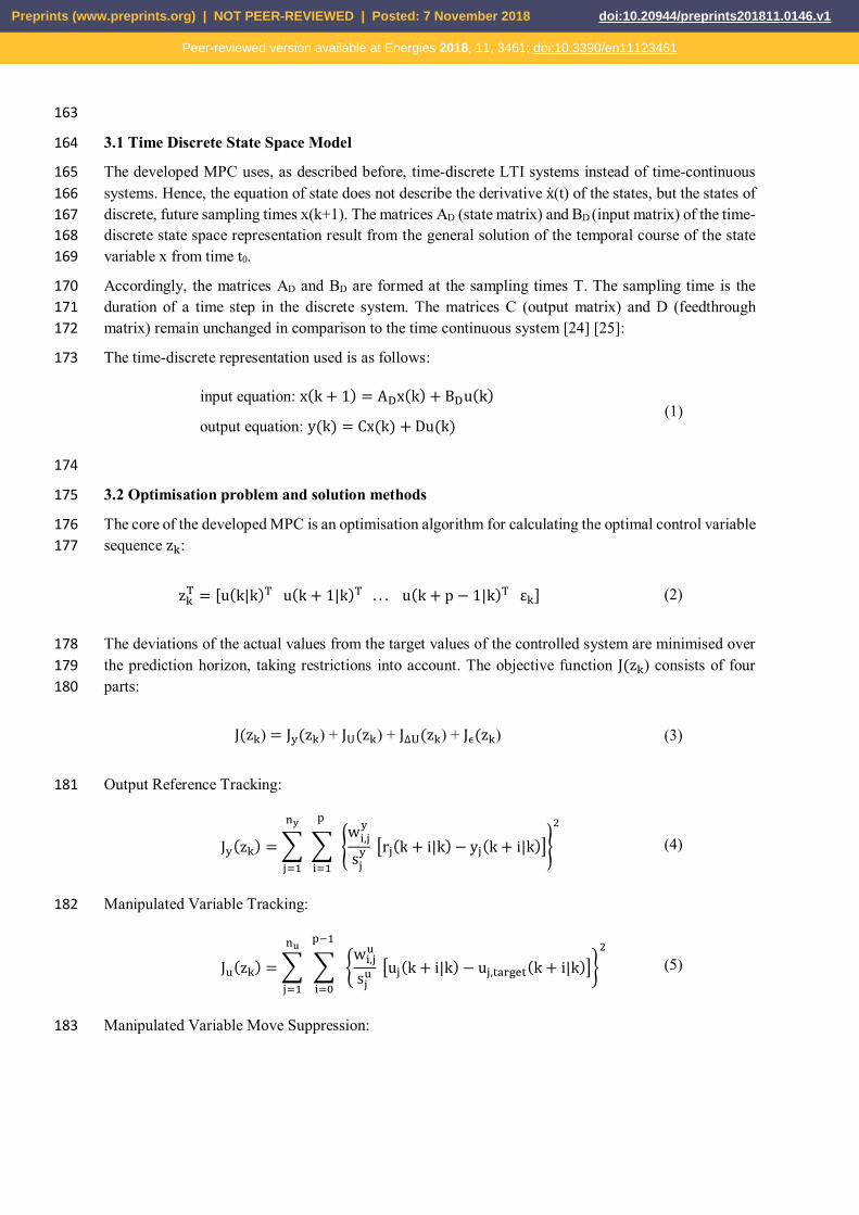
In order to be able to model the hall, extensive measurements were carried out and physical models of 225 the hall and the technical building equipment were created in MATLAB/SIMLUNK. The most 226 important parameters for modelling the system can be found in the table below. 227

228

Table 1: Important key parameters of the modelled packaging hall 229

Parameter packaging hall Value Unit Room volume 800 m

Supply air volume flow 2000 mh

Heat transfer coefficient walls/ceiling 0.28 Wm K

Heat transfer coefficient floor 1.00 Wm K

Ground temperature 15 °C

Storage capacity, medium according to DIN V 18599-2 [29] 90 Whm K

Inner thermal load (during production) 1292 W

Humidity entry max. (during production) 48 gh

230

The models used for the room, the air conditioning system and the boundary parameters (internal loads, 231 electricity prices, weather) are described below. 232

233

4.1 Physical building model 234

The physical room model used is based on a building model from the CARNOT toolbox (Conventional 235 And Renewable eNergy systems Optimisation Toolbox) [30], which is freely available for 236 MATLAB/SIMUNLINK. 237

The thermal heat-up and cooling behaviour is calculated by integrating the heat flow balance ∑ Q 238 divided by the thermal storage capacity of the building mass m ∙ c over time. 239

ϑ(t) =∑ Qm ∙ c

dt (9)




http://dx.doi.org/10.3390/en11123461

The change of the absolute air humidity is calculated analogously to the thermal behaviour. 240

241

4.2 Physical air conditioning system model 242

The HVAC system consists of an electric pre- and post-heater, a cooling register, which is supplied 243 with cold by a compression chiller, an electrically operated steam humidifier, a supply and exhaust fan 244 and is operated with 100% fresh air. 245

The HVAC simulation model is based on the physical laws of the Mollier diagram [31]. Furthermore, 246 characteristic curves of the manufacturer are used for modelling the cooling supply (compression chiller 247 with flow temperature of -1 °C) and steam humidification (3 bar of saturated steam). 248

249

4.3 Boundary parameters - internal load 250

The internal thermal and water loads necessary for an optimised, model-predictive control of an air 251 conditioning system are determined by real active power measurements of the machines in the hall, 252 calculations for the heat of illumination according to VDI 2078 [31], humidity and heat emission of the 253 persons in the hall according to VDI 2078 and the influence of the local air conditioning by transfer of 254 laboratory results. 255

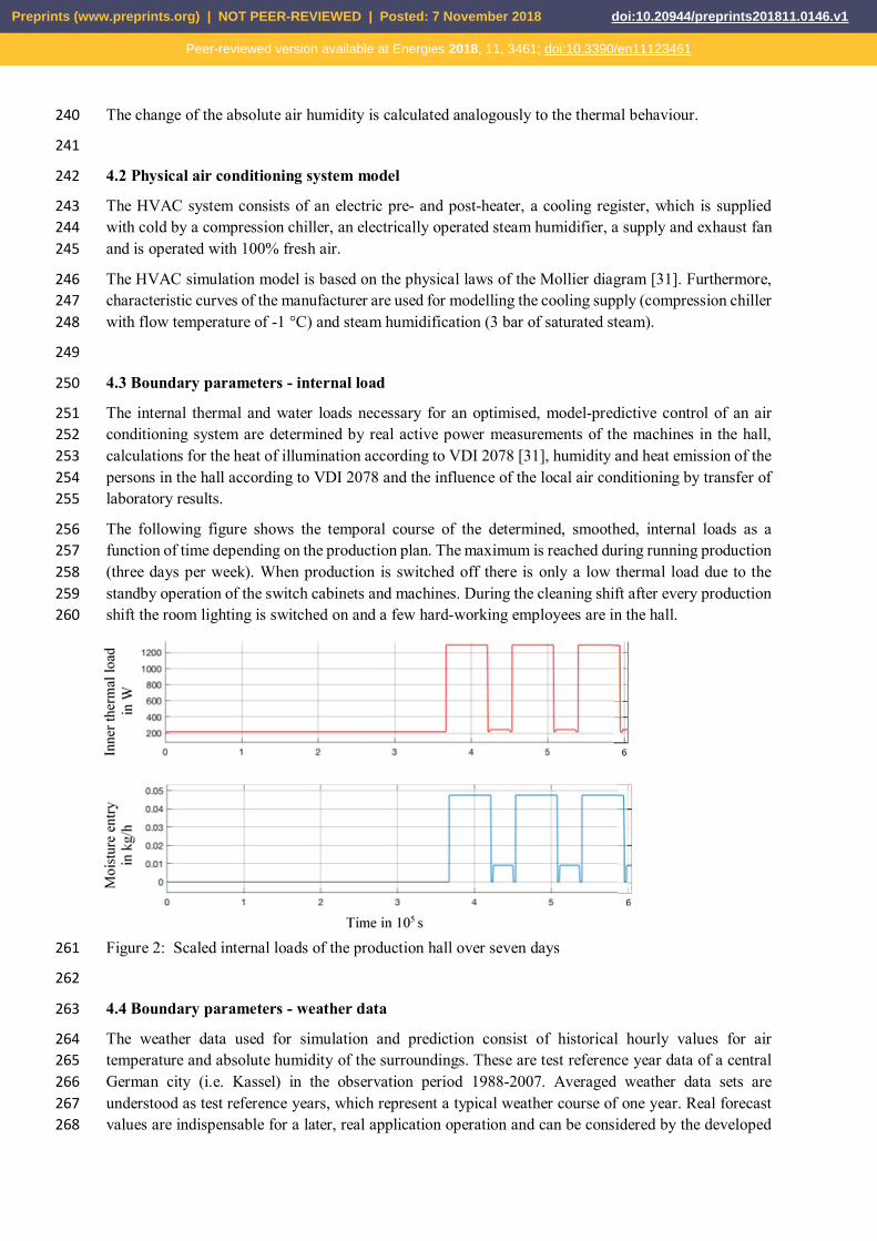
The following figure shows the temporal course of the determined, smoothed, internal loads as a 256 function of time depending on the production plan. The maximum is reached during running production 257 (three days per week). When production is switched off there is only a low thermal load due to the 258 standby operation of the switch cabinets and machines. During the cleaning shift after every production 259 shift the room lighting is switched on and a few hard-working employees are in the hall. 260

Figure 2: Scaled internal loads of the production hall over seven days 261

262

4.4 Boundary parameters - weather data 263

The weather data used for simulation and prediction consist of historical hourly values for air 264 temperature and absolute humidity of the surroundings. These are test reference year data of a central 265 German city (i.e. Kassel) in the observation period 1988-2007. Averaged weather data sets are 266 understood as test reference years, which represent a typical weather course of one year. Real forecast 267 values are indispensable for a later, real application operation and can be considered by the developed 268




http://dx.doi.org/10.3390/en11123461

control. However, historical weather data sets is used to determine savings and flexibility potentials, as 269 these can cover a long period of time and reflect the expected value without annual deviations. 270

271

4.5 Boundary parameters - electricity price data 272

Two electricity price scenarios are defined for the analysis of an economic, model predictive control, a 273 constant and a flexible model: 274

1. In the status quo scenario a standard, constant total electricity price (13.18 ct/kWh) for industrial 275 customers in Germany is chosen. 276

2. In opposite to that, the second scenario reflects a possible future electricity price model of a 277 dynamized renewable energy levy (EEG levy) and electricity procurement via the day-ahead 278 exchange market in Germany. The current static EEG levy due in Germany, which is levied to 279 promote renewable energies in Germany, is replaced by a dynamic EEG levy, which is calculated 280 via the day-ahead exchange electricity price using a certain factor. 281

퐹푙푒푥푖푏푙푒퐸퐸퐺푙푒푣푦 = 퐷푎푦-푎ℎ푒푎푑푒푙푒푐푡푟푖푐푡푦푝푟푖푐푒 ∙ 푚푢푙푡푖푝푖푒푟 282

This multiplier must be successively recalculated and determined for the differential cost 283 compensation for Germany. For the following simulations, a factor of 1.9 has been defined. 284 Furthermore, limits of the flexible EEG allocation upwards and downwards are foreseen. The upper 285 limit of the dynamic EEG levy consists of twice the German, static EEG levy, the lower limit is 0, 286 negative electricity prices are no longer possible according to this model. [32] [33] 287

In addition to the electricity price incidental electricity costs are considered in all analysed scenarios 288 corresponding to the average costs of 4.28 ct/kWh for German industrial customers with an annual 289 consumption of 160 to 20,000 MWh [34]. 290

The exchange electricity price generally has two maximums and two minimums per day. Since the loads 291 are to be shifted from a high tariff to a tariff as low as possible, a prediction of at least 12 hours is 292 necessary. Regarding a time step of 900 s and a prediction horizon of 12 hours, this results in 48 293 prediction steps. To reduce calculation efforts the control horizon is set to 20 steps, i.e. 5 hours. 294

Comparable to the weather forecast, real electricity price forecast is also indispensable for real 295 operation. The electricity price forecast is included in the developed MPC approach by downloading 296 real electricity prices from EEX for the next day (day-ahead electricity prices) and script-based further 297 processing. However, as already described in the section on weather forecasting, historical electricity 298 price time series over longer periods are better suited for calculating flexibility and savings calculations. 299

300

4.6 MPC constraints 301

The constraints used to create the MPC do not vary in all considered scenarios. The constraints include 302 the permissible temperature and humidity limits in the room as well as the control variable limitation. 303 Both, the temperature as well as the air humidity depend on the limits of an average comfort field. The 304 control variable limitation resulting from the air conditioning system control are as follows: 305

16°C ≤ Room temperature ≤ 24°C 306

0,005 kg/kg ≤ Absolute humidity Room ≤ 0,009 kg/kg 307

0 ≤ Control variable heating/moisture/cooling ≤ 1 308

309




http://dx.doi.org/10.3390/en11123461

4.7 MPC weights 310

The different weights of the sub-target functions that are required to create the MPC are described 311 below. In all scenarios, the control variables should not adhere to a value and therefore have a weight 312 of 0. The weight of the change suppression of the control variables is set to 0.1. This reduces the upswing 313 and downswing of the control values that is too fast. 314

The weightings of the control variables vary depending on the scenario, which are described in section 315 5. A distinction is made between two cases: 316

1. The energy-optimal control keeps the indoor temperature and humidity above limits in the comfort 317 field. The weights of the first two model outputs (indoor temperature and absolute humidity) are 0. 318 The third output (i.e. power) is to be minimised hence it receives a weight of 1. 319

2. The regulation with economic objective function receives quasi the current electricity price as 320 weight for the achievement. This is multiplied by 10, since this setting thus has a similar weight as 321 with the energy-optimal regulation and better results are obtained. The temperature and humidity 322 of the room are no longer included in the target function. 323

324

5. Scenario description and results 325

In order to evaluate the flexibility and savings potentials, the previously described control variants of 326 the MPC at different seasons are analysed. 327

First, three days in January are graphically examined in order to illustrate a possible load shift (scenario 328 I-III). Subsequently, electricity consumption and costs incurred by the three different operating variants 329 are compared over 20 days in January. Since the weather influences change strongly in the summer, the 330 load management potential is finally illustrated by a flexible electricity price and EMPC for 10 days in 331 July. 332

The energy-optimal scenario I serves as a comparison for the scenarios in which load management is 333 carried out. Scenarios II and III use the economic objective function in which the current AHU system 334 output multiplied by the current electricity price over the prediction horizon is minimized. In the second 335 scenario a constant electricity price is assumed, in the third scenario a flexible electricity price as 336 described above is used. Table 1 shows an overview of the simulated scenarios. 337

338

Table 2: Overview of the simulated scenarios 339

Scenario Objective function Weights [temp. humidity power/costs]

I. Energy-optimised MPC energy-optimised [0 0 1] II. EMPC with constant electricity price

economic-optimised [0 0 p ∙ k ]

III. EMPC with flexible electricity price economic-optimised [0 0 p ∙ k ]]

340

5.1 Comparison scenario I: Energy-optimised MPC - 3 days in January 341

In this scenario, the energy consumption of the air conditioning system is minimized. The weights for 342 temperature and absolute humidity are 0. The comfort field is maintained by the restrictions. The weight 343 for the performance of the system components is 1. The weight for the output of the system components 344




http://dx.doi.org/10.3390/en11123461

is 1. The target value for the output is 0. Thus, the summed quadratic deviation of the power from 0 345 over the prediction horizon is minimized. 346

As shown in figure 4, the room temperature is kept at the lowest limit of 16°C, as this is the least amount 347 of energy required for supply air conditioning. The absolute humidity of the outside air is not raised by 348 the humidifier if it is above the lower limit of 5 g/kg. Since the HVAC system is operated with 100 % 349 fresh air from the outside, the absolute humidity of the room, provided that it remains within the 350 specified limits, depends on the conditions of the fresh air, as can be seen in area 1 of figure 4. 351

Figure 3: Energy-optimised MPC over three days in January 352

353

5.2 Scenario II: Cost-optimised MPC (EMPC) with constant electricity price - 3 days in January 354

In this scenario, the economic objective function is used to minimize costs. The output is multiplied by 355 the current costs in each time step and minimized by adding up the prediction horizon. The electricity 356 price in this scenario is constant at 13.18 ct/kWh. Therefore, this is a simultaneous energetic and 357 economic optimisation. The difference between this regulation and the regulation in scenario I is that 358 the current power consumption of the air conditioning system is no longer included in the target function 359 as a square but linear value. As a result, energy cost peaks are no longer minimized, as they no longer 360 flow disproportionately into the target function. 361

The behaviour is very similar to the previous scenario I. However, in contrast to scenario I, the heating 362 coil remains switched off during the first hours (area 1, figure 5), so that the room temperature drops 363 more quickly (area 2, figure 5). The room air restrictions 364

365




http://dx.doi.org/10.3390/en11123461

Figure 4: Energy-optimised and cost-optimised EMPC with constant electricity price over three days in 366 January 367

368

5.3 Scenario III: Cost-optimised MPC with flexible electricity price - 3 days in January 369

In this scenario, a flexible electricity price is used as described in Section 4.6. This results in electricity 370 price changes of up to 10 cents (figure 6). The indoor temperature varies between 16 and 21°C. The 371 control variables of the heating coil vary between 0 and 1. Especially in low-price phases (area 1, figure 372 6) and before a sudden price increase, the heating register (area 2, figure 6) prematurely heats up the 373 room (area 3, figure 6). The humidifier is only activated when the absolute humidity falls below 5g/kg. 374 Load shifts are possible s shown in figure 6. 375




http://dx.doi.org/10.3390/en11123461

Figure 5: Cost-optimised EMPC with flexible electricity price over three days in January 376

377

5.4 Winter case - comparison of control variants over 20 days in January 378

Three scenarios were simulated over the first 20 days in January of the reference year. The energy 379 consumption and the energy costs incurred by the air conditioning system are shown in Table 2. The 380 relevant changes are also shown. 381

The comparison between energy-optimised control and EMPC already shows a reduction in energy 382 consumption and a resulting cost reduction of 2.14%. Scenario III, with lower energy consumption, will 383 henceforth be used as a comparison scenario. 384

The results of the simulation with dynamic EEG allocation show a reduction in costs of 2.10% compared 385 to the energy-optimal scenario with changed target function and constant electricity price. However, 386 energy consumption increases by 7.44%. This higher energy consumption is due to the fact that the 387 room temperature for storing the shifted energy is raised, resulting in higher heat losses. 388

389




http://dx.doi.org/10.3390/en11123461

Table 3: Energy consumption and costs over 20 days in January under different scenarios 390

Scenario 20 days Consumption in kWh Costs in € I Energy-optimised MPC 3926 517.3 II EMPC with constant electricity price 3842 506.4 Change: I → II -2.14% -2.14% III Flexible EEG-Levy 4128 498.9 Change: II→ III +7.44% -2.10%

391

5.5 Summer case - EMPC with flexible electricity price over 10 days in July 392

In addition to the winter case, 10 days in summer (days 191-200) are simulated with an electricity price 393 including dynamic EEG allocation (see scenario III). It is investigated, to which extent the cooling 394 register can contribute to load management. The results are shown in figure 7. 395

In summer most of the energy is needed to dehumidify the supply air (area 1, figure 7). Since the room 396 air is exchanged relatively fast it is not possible to store energy by shifting the dehumidification output. 397 There is no correlation between the electricity price and the control signal of the cooling register. The 398 outside air is cooled by dehumidification. Therefore, despite high outside temperatures, low inside 399 temperatures must be noted (area 2, figure 7). A shift before cooling loads is therefore also not possible 400 and load management cannot be carried out under such weather conditions. 401




http://dx.doi.org/10.3390/en11123461

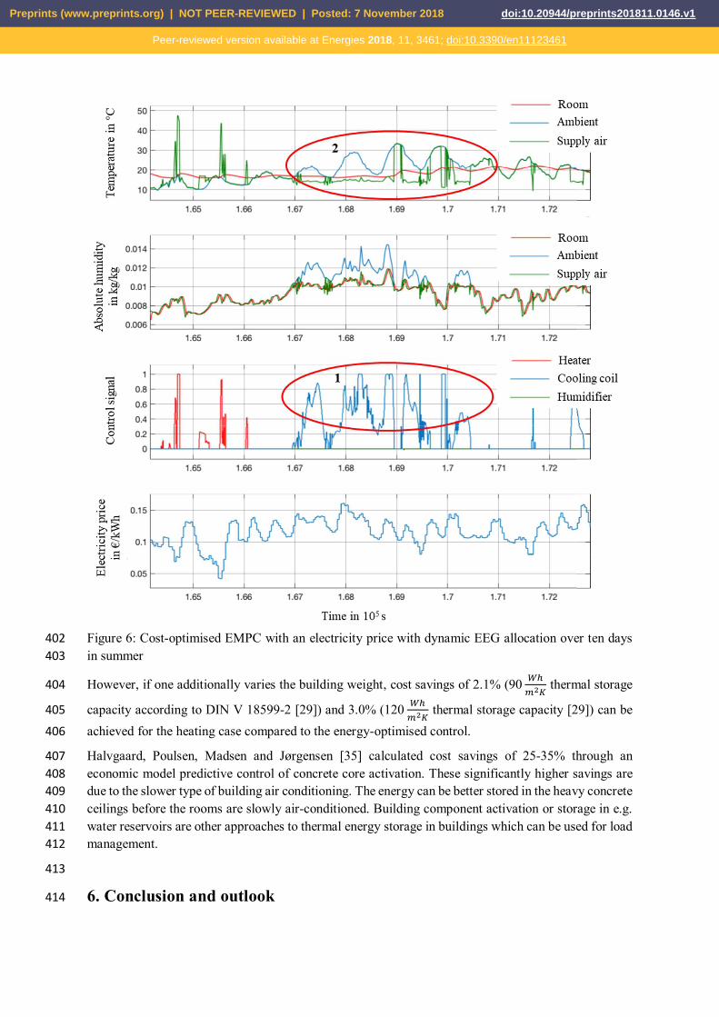
Figure 6: Cost-optimised EMPC with an electricity price with dynamic EEG allocation over ten days 402 in summer 403

However, if one additionally varies the building weight, cost savings of 2.1% (90 thermal storage 404

capacity according to DIN V 18599-2 [29]) and 3.0% (120 thermal storage capacity [29]) can be 405

achieved for the heating case compared to the energy-optimised control. 406

Halvgaard, Poulsen, Madsen and Jørgensen [35] calculated cost savings of 25-35% through an 407 economic model predictive control of concrete core activation. These significantly higher savings are 408 due to the slower type of building air conditioning. The energy can be better stored in the heavy concrete 409 ceilings before the rooms are slowly air-conditioned. Building component activation or storage in e.g. 410 water reservoirs are other approaches to thermal energy storage in buildings which can be used for load 411 management. 412

413

6. Conclusion and outlook 414




http://dx.doi.org/10.3390/en11123461

The paper illustrates an economic multiple model predictive control of a HVAC that can either meet 415 room temperature and humidity targets, minimise energy consumption or alternatively minimise 416 economic costs through a flexible electricity pricing model. 417

As a case study, a production hall for the packaging of chocolate bars is used, which are locally air-418 conditioned by a cross-flowing displacement ventilation for conveyor belts, so that the room air 419 condition can be kept within a comfort zone with the help of restrictions and does not have to depend 420 on the product requirements of the chocolate (18°C, 50% relative humidity) [12]. The internal loads of 421 the production hall as well as weather data influence the system as disturbance variables and are taken 422 into account by the MPC controller. To evaluate the EMMPC controller, various scenarios are evaluated 423 taking seasonal weather influences into account. 424

Electricity costs in winter can thus be reduced by 2.1% compared to energy-optimised control. 425 However, energy consumption increases by 7.44% due to higher heat losses when the room temperature 426 is temporarily raised. It could also be shown that a larger thermal storage capacity of the building can 427 increase the potential for load shifting. 428

For example, in order to be able to include a mixed air chamber, which causes even stronger non-429 linearities in the system behaviour, in a MPC control system, the extension of the MMPC by further 430 MPC controllers is currently being worked on. In addition, the coupling to a production plan-dependent 431 activation time optimisation adapted to the hall and outdoor air conditions, which determines an optimal 432 start time for the air-conditioning of the hall, is in progress. In this way, energy consumption can be 433 further reduced [13]. 434

In order to demonstrate the functionality also in real operation, the coupling with full HVAC system 435 with connected climate chamber, in which also internal loads can be simulated, is under construction. 436 A further starting point is the creation of adaptive, self-learning state space models, which are generated 437 on the basis of real measurement data in order to further improve the prognostic capability and thus the 438 accuracy of the optimal control variables. 439

The publication shows that the use of an economic model predictive control is suitable for the efficient 440 and economic prognostic guided control of HVAC plants, which could actively participate in load 441 management. It is also shown that the approach of a multiple model predictive control can particularly 442 control non-linear behaviour of typical HVAC processes like dry and wet cooling. Thus, EMMPC can 443 be seen as a promising approach to optimise the flexible operation of complex HVAC systems. 444 However, even more in-depth development work is required to map even more complex systems on the 445 one hand and to be able to control real systems in real time on the other. 446

447

Acknowledgments 448

The contents of this paper have been acquired within the cooperation project „Smart Consumer – Energy 449 efficiency through systemic coupling of energy flows by means of intelligent measurement and control 450 technology”. The Project is funded by the German Federal Ministry for Economic Affairs and Energy 451 (FKZ: 03ET1180). 452

453

454

455

456




http://dx.doi.org/10.3390/en11123461

Nomenclature 457

x(t): State vector 458

u(t): System input vector 459

y(t): System output vector 460

A: State matrix 461

B: Input matrix 462

C: Output matrix 463

D: Feedthrough matrix 464

y: Plant output 465

u: Manipulated variable 466

z : Optimal control variable sequence 467

J(z ): Objective function 468

n: Number of plant output variables or manipulated variables 469

p: Prediction horizon (number of intervals) 470

w: Tuning weight 471

s: Scale factor 472

r: Reference 473

k: Current control interval 474

ρ : Constraint violation penalty weight 475

ϵ : Slack variable at control interval k 476

∑ Q: Heat flow balance in W 477

m: Building mass in kg 478

c : Specific heat capacity at constant pressure J/kg ∙ K 479

ϑ(t): Temperature at time t 480

t: Time in s 481

P : Total power consumption of the HVAC system (without fan power consumption) in kW 482

k : Electricity price in (€/kWh)/s 483

484

485

486

487

488

489




http://dx.doi.org/10.3390/en11123461

References 490

[1] United Nations, Climate Change, available at http://www.un.org/en/sections/issues-491 depth/climate-change (accessed on October 2018). 492

[2] NASA, Global Climate Change - Vital Signs of the Planet, available at https://climate.nasa.gov/ 493 (accessed on October 2018). 494

[3] R.K. Pachauri, L. Mayer (Eds.), Climate change 2014: Synthesis report, Intergovernmental Panel 495 on Climate Change, Geneva, Switzerland, 2015. 496

[4] A.P. Patwardhan, L. Gomez-Echeverri, N. Nakićenović, T.B. Johansson (Eds.), Global Energy 497 Assessment (GEA), Cambridge University Press, Cambridge, 2012. 498

[5] L. D&R International, 2011 Buildings Energy Data Book, Pacific Northwest National 499 Laboratory, 2012. 500

[6] L. Pérez-Lombard, J. Ortiz, C. Pout, A review on buildings energy consumption information, 501 Energy and Buildings 40 (3) (2008) 394–398. 502

[7] G. Guyot, M.H. Sherman, I.S. Walker, Smart ventilation energy and indoor air quality 503 performance in residential buildings: A review, Energy and Buildings 165 (2018) 416–430. 504

[8] R. Hitchin, C. Pout, D. Butler, Realisable 10-year reductions in European energy consumption 505 for air conditioning, Energy and Buildings 86 (2015) 478–491. 506

[9] K. Zhang, X. Zhang, S. Li, X. Jin, Review of underfloor air distribution technology, Energy and 507 Buildings 85 (2014) 180–186. 508

[10] H. Meschede, Increased utilisation of renewable energies through demand response in the water 509 supply sector – a case study, Rio de Janeiro, Brazil, 2018. 510

[11] D. Khripko, S.N. Morioka, S. Evans, J. Hesselbach, M.M. de Carvalho, Demand Side 511 Management within Industry: A Case Study for Sustainable Business Models, Procedia 512 Manufacturing 8 (2017) 270–277. 513

[12] T. Heidrich, A. Alimi, L. Grothues, J. Hesselbach, O. Wünsch, Cross-flowing displacement 514 ventilation system for conveyor belts in the food industry, Energy and Buildings 179 (2018) 515 213–222. 516

[13] T. Heidrich, H. Dunkelberg, T. Weiß, J. Hesselbach, Flexibilization of Energy Supply Using the 517 Example of Industrial Hall Climatization and Cold Production, Kassel University Press GmbH, 518 Kassel, 2017. 519

[14] J. Wagner, Lokale Klimatisierung temperatursensibler Produkte. Dissertation, Kassel University 520 Press GmbH, Kassel, 2016. 521

[15] T. Heidrich, Energieeffizienzsteigerung in der Süßwarenindustrie durch lokale Klimatisierung 522 und systemische Kopplung von Energieströmen. DLG session - innovative energy technologies 523 in the food industry, Hannover 2016. 524

[16] A. Afram, F. Janabi-Sharifi, Theory and applications of HVAC control systems – A review of 525 model predictive control (MPC), Building and Environment 72 (2014) 343–355. 526

[17] D.S. Naidu, C.G. Rieger, Advanced control strategies for HVAC&R systems—An overview: 527 Part II: Soft and fusion control, HVAC&R Research 17 (2) (2011) 144–158. 528




http://dx.doi.org/10.3390/en11123461

[18] A.E. Ruano, S. Pesteh, S. Silva, H. Duarte, G. Mestre, P.M. Ferreira, H.R. Khosravani, R. Horta, 529 The IMBPC HVAC system: A complete MBPC solution for existing HVAC systems, Energy 530 and Buildings 120 (2016) 145–158. 531

[19] K.F. Früh, D. Schaudel, U. Maier, R. Bleich (Eds.), Handbuch der Prozessautomatisierung: 532 Prozessleittechnik für verfahrenstechnische Anlagen, 5th ed., DIV Dt. Industrieverl., München, 533 2015. 534

[20] Y. Ma, A. Kelman, A. Daly, F. Borrelli, Predictive Control for Energy Efficient Buildings with 535 Thermal Storage: Modeling, Stimulation, and Experiments, IEEE Control Syst. 32 (1) (2012) 536 44–64. 537

[21] F. Belic, Z. Hocenski, D. Sliskovic, HVAC Control Methods - A review. 19th International 538 Conference on System Theory, Control and Computing (ICSTCC), 2015 October 14-16, Cheile 539 Gradistei, Romania. 540

[22] A. Bemporad, M. Morari, N.L. Ricker, Model Predictive Control Toolbox – Getting Started 541 Guide, 2017. 542

[23] A. Bemporad, M. Morari, N.L. Ricker, Model Predictive Control Toolbox – User’s Guide, 2017. 543

[24] J. Lunze, Regelungstechnik 2: Mehrgrößensysteme, Digitale Rechnung, 8th ed., Springer 544 Vieweg, Berlin, 2014. 545

[25] J. Lunze, Regelungstechnik 1: Systemtheoretische Grundlagen, Analyse und Entwurf 546 einschleifiger Regelungen, 6th ed., Springer, Berlin, 2007. 547

[26] J. Nocedal, S.J. Wright, Numerical Optimization, Springer Science+Business Media LLC, New 548 York, NY, 2006. 549

[27] S. Schirmer, T. Heidrich, J. Wagner, J. Hesselbach, Steigerung der Energieeffizienz einer 550 klimatisierten Produktionshalle, HLH (July/August) (2016) 38–40. 551

[28] J. Wagner, M. Schäfer, A. Schlüter, L. Harsch, J. Hesselbach, M. Rosano, C.-X. Lin, Reducing 552 energy demand in production environment requiring refrigeration—A localized climatization 553 approach, HVAC&R Research 20 (6) (2014) 628–642. 554

[29] German engineering standard, DIN V 18599-2: 2011-12 - Energy assessment of buildings - 555 Calculation of the useful, final and primary energy demand for heating, cooling, ventilation, 556 domestic hot water and lighting - Part 2: Useful energy demand for heating and cooling of 557 building zones. 558

[30] FH Aachen, CARNOT Toolbox 2018, available at https://fh-559 aachen.sciebo.de/index.php/s/0hxub0iIJrui3ED and 560 https://de.mathworks.com/matlabcentral/fileexchange/68890-carnot-toolbox (accessed on 561 October 2018). 562

[31] Association of German Engineers, VDI-Wärmeatlas, 11th ed., Springer Vieweg, Berlin, 2013. 563

[32] Frontier Economics, Costs and benefits of dynamizing electricity price components as a means 564 of making demand more flexible, 2016 Report for the German federal ministry of Economics 565 and Energy (BMWi), Frontier Economics Ltd, London. 566

[33] Dr. Thies F. Clausen, Der Spotmarktpreis als Index für eine dynamische EEG - Umlage, Talk at 567 AG Flexibility of the BMWi, August 19th 2014, Berlin, available at https://www.agora-568 energiewende.de/veroeffentlichungen/der-spotmarktpreis-als-index-fuer-eine-dynamische-eeg-569 umlage/ (accessed on October 2018). 570




http://dx.doi.org/10.3390/en11123461

[34] BDEW (Federal Association of Energy and Water Management), Composition of electricity 571 prices for industry in Germany in 2016 and 2017, available at 572 https://de.statista.com/statistik/daten/studie/168571/umfrage/strompreis-fuer-die-industrie-in-573 deutschland-seit-1998/ (accessed on October 2018). 574

[35] R. Halvgaard, N.K. Poulsen, H. Madsen, J.B. Jorgensen, Economic Model Predictive Control for 575 building climate control in a Smart Grid, in: IEEE PES innovative smart grid technologies 576 (ISGT), 2012: Conference] ; 16 - 20 Jan. 2012, Washington, DC, USA, Washington, DC, USA, 577 IEEE, Piscataway, NJ, 2012, pp. 1–6. 578

579




http://dx.doi.org/10.3390/en11123461

Documents

Economic multiple model predictive control for HVAC