ECONOMIC OPERATION OF POWER SYSTEMS - …€¦ · 3 Fig .2 Heat rate curve. INCREMENTAL FUEL RATE CURVE The incremental fuel rate is equal to a small change in input divided by the

1

ECONOMIC OPERATION OF POWER SYSTEMS

INTRODUCTION One of the earliest applications of on-line centralized control was to provide a central

facility, to operate economically, several generating plants supplying the loads of the

system. Modern integrated systems have different types of generating plants, such as coal

fired thermal plants, hydel plants, nuclear plants, oil and natural gas units etc. The capital

investment, operation and maintenance costs are different for different types of plants.

The operation economics can again be subdivided into two parts.

i) Problem of economic dispatch, which deals with determining the power

output of each plant to meet the specified load, such that the overall fuel cost

is minimized.

ii) Problem of optimal power flow, which deals with minimum – loss delivery,

where in the power flow, is optimized to minimize losses in the system. In

this chapter we consider the problem of economic dispatch.

During operation of the plant, a generator may be in one of the following states:

i) Base supply without regulation: the output is a constant.

ii) Base supply with regulation: output power is regulated based on system load.

iii) Automatic non-economic regulation: output level changes around a base

setting as area control error changes.

iv) Automatic economic regulation: output level is adjusted, with the area load

and area control error, while tracking an economic setting.

Regardless of the units operating state, it has a contribution to the economic operation,

even though its output is changed for different reasons. The factors influencing the cost

of generation are the generator efficiency, fuel cost and transmission losses. The most

efficient generator may not give minimum cost, since it may be located in a place where

fuel cost is high. Further, if the plant is located far from the load centers, transmission

losses may be high and running the plant may become uneconomical. The economic

dispatch problem basically determines the generation of different plants to minimize total

operating cost.

www.bookspar.com | VTU NOTES | QUESTION PAPERS | NEWS | RESULTS | FORUMS


2

Modern generating plants like nuclear plants, geo-thermal plants etc, may require capital

investment of millions of rupees. The economic dispatch is however determined in terms

of fuel cost per unit power generated and does not include capital investment,

maintenance, depreciation, start-up and shut down costs etc.

PERFORMANCE CURVES INPUT-OUTPUT CURVE This is the fundamental curve for a thermal plant and is a plot of the input in British

thermal units (Btu) per hour versus the power output of the plant in MW as shown in Fig

1.

Btu

/ hr

(Inp

ut)

(output) MW Fig 1: Input – output curve

HEAT RATE CURVE The heat rate is the ratio of fuel input in Btu to energy output in KWh. It is the slope of

the input – output curve at any point. The reciprocal of heat – rate is called fuel –

efficiency. The heat rate curve is a plot of heat rate versus output in MW. A typical plot

is shown in Fig .2

(output) MW

(Hea

t rat

e) B

tu /

kw-h

r



3

Fig .2 Heat rate curve. INCREMENTAL FUEL RATE CURVE The incremental fuel rate is equal to a small change in input divided by the

corresponding change in output.

Incremental fuel rate =OutputInput

∆∆

The unit is again Btu / KWh. A plot of incremental fuel rate versus the output is shown in

Fig 3

(output) MW

Incr

emen

tal f

uel r

ate

Fig 3: Incremental fuel rate curve Incremental cost curve The incremental cost is the product of incremental fuel rate and fuel cost (Rs / Btu or $ /

Btu). The curve in shown in Fig. 4. The unit of the incremental fuel cost is Rs / MWh or

$ /MWh.



4

(output) MW

approximate linear cost

actual cost

Rs

/ Mw

hr

Fig 4: Incremental cost curve

In general, the fuel cost Fi for a plant, is approximated as a quadratic function of the

generated output PGi.

Fi = ai + bi PGi + ci PGi

2 Rs / h

The incremental fuel cost is given by

Gi

i

dPdF

= bi + 2ci PGi Rs / MWh

The incremental fuel cost is a measure of how costly it will be produce an increment of

power. The incremental production cost, is made up of incremental fuel cost plus the

incremental cost of labour, water, maintenance etc. which can be taken to be some

percentage of the incremental fuel cost, instead of resorting to a rigorous mathematical

model. The cost curve can be approximated by a linear curve. While there is negligible

operating cost for a hydel plant, there is a limitation on the power output possible. In any

plant, all units normally operate between PGmin, the minimum loading limit, below which

it is technically infeasible to operate a unit and PGmax, which is the maximum output

limit.

ECONOMIC GENERATION SCHEDULING NEGLECTING LOSSES AND GENERATOR LIMITS The simplest case of economic dispatch is the case when transmission losses are

neglected. The model does not consider the system configuration or line impedances.

Since losses are neglected, the total generation is equal to the total demand PD.



5

Consider a system with ng number of generating plants supplying the total

demand PD. If Fi is the cost of plant i in Rs/h, the mathematical formulation of the

problem of economic scheduling can be stated as follows:

Minimize FT = �=

gn

iiF

1

Such that D

n

iGi PP

g

=�=1

where FT = total cost. PGi = generation of plant i. PD = total demand. This is a constrained optimization problem, which can be solved by Lagrange’s method. LAGRANGE METHOD FOR SOLUTION OF ECONOMIC SCHEDULE The problem is restated below:

Minimize �=

=gn

iiT FF

1

Such that 01

== �=

gn

iGiD PP

The augmented cost function is given by

��

��

�−+= �

=

gn

iGiD PP

1TF £ λ

The minimum is obtained when

0£ =

∂∂

GiP and 0

£ =∂∂λ

0P£

Gi

=−∂∂

=∂∂ λ

Gi

T

PF

0£

1

=−=∂∂

�=

gn

iGiD PP

λ



6

The second equation is simply the original constraint of the problem. The cost of a plant

Fi depends only on its own output PGi, hence

Gi

i

Gi

i

Gi

T

dPdF

PF

PF

=∂∂

=∂∂

Using the above,

λ==∂∂

Gi

i

Gi

i

dPdF

PF

; i = 1……. ng

We can write

bi + 2ci PGi = λ i = 1……. ng The above equation is called the co-ordination equation. Simply stated, for economic

generation scheduling to meet a particular load demand, when transmission losses are

neglected and generation limits are not imposed, all plants must operate at equal

incremental production costs, subject to the constraint that the total generation be equal

to the demand. From we have

i

iGi c

bP

2−

=λ

We know in a loss less system

D

n

iGi PP

g

=�=1

Substituting (8.16) we get

D

n

i i

i Pcbg

=−�

=1 2λ

An analytical solution of � is obtained from (8.17) as

�

�

=

=

+=

g

g

n

i i

n

i i

iD

c

cb

P

1

1

21

2λ

It can be seen that λ is dependent on the demand and the coefficients of the cost function.

Example 1.

The fuel costs of two units are given by



7

F1 = 1.5 + 20 PG1 + 0.1 PG12 Rs/h

F2 = 1.9 + 30 PG2 + 0.1 PG22 Rs/h

PG1, PG2 are in MW. Find the optimal schedule neglecting losses, when the demand is

200 MW.

Solution:

11

1 2.020 GG

PdPdF

+= Rs / MWh

22

2 2.030 GG

PdPdF

+= Rs / MWh

20021 =+= GGD PPP MW

For economic schedule

λ==2

2

1

1

GG dPdF

dPdF

20 + 0.2 PG1 = 30 + 0.2 (200 - PG1)

Solving we get, PG1 = 125 MW

PG2 = 75 MW

λ = 20 + 0.2 (125) = 45 Rs / MWh

Example 2

The fuel cost in $ / h for two 800 MW plants is given by

F1 = 400 + 6.0 PG1 + 0.004 PG12

F2 = 500 + b2 PG2 + c2 PG22

where PG1, PG2 are in MW

(a) The incremental cost of power, λ is $8 / MWh when total demand is 550MW.

Determine optimal generation schedule neglecting losses.

(b) The incremental cost of power is $10/MWh when total demand is 1300 MW.

Determine optimal schedule neglecting losses.

(c) From (a) and (b) find the coefficients b2 and c2.

Solution:

a) 250004.02

0.60.82 1

11 =

×−=

−=

cb

PG

λ MW

30025055012 =−=−= GDG PPP MW



8

b) 500004.02610

2 1

11 =

×−=

−=

Cb

PG

λ MW

800500130012 =−=−= GDG PPP MW

c) 2

22 2c

bPG

−=

λ

From (a) 2

2

20.8

300c

b−=

From (b) 2

2

20.10

800c

b−=

Solving we get b2 = 6.8 c2 = 0.002 ECONOMIC SCHEDULE INCLUDING LIMITS ON GENERATOR (NEGLECTING LOSSES) The power output of any generator has a maximum value dependent on the rating of the

generator. It also has a minimum limit set by stable boiler operation. The economic

dispatch problem now is to schedule generation to minimize cost, subject to the equality

constraint.

D

n

iGi PP

g

=�=1

and the inequality constraint

PGi (min) � PGi � PGi (max) ; i = 1, ……… ng The procedure followed is same as before i.e. the plants are operated with equal

incremental fuel costs, till their limits are not violated. As soon as a plant reaches the

limit (maximum or minimum) its output is fixed at that point and is maintained a

constant. The other plants are operated at equal incremental costs.

Example 3

Incremental fuel costs in $ / MWh for two units are given below:

0.201.0 11

1 += GG

PdPdF

$ / MWh



9

6.1012.0 22

2 += GG

PdPdF

$ / MWh

The limits on the plants are Pmin = 20 MW, Pmax = 125 MW. Obtain the optimal schedule

if the load varies from 50 – 250 MW.

Solution: The incremental fuel costs of the two plants are evaluated at their lower limits and upper

limits of generation.

At PG (min) = 20 MW.

1

1(min)1

GdPdF

=λ = 0.01x 20+2.0 = 2.2$ / MWh

2

2(min)2

GdPdF

=λ = 0.012 x 20 + 1.6 = 1.84 $ / MWh

At PG (Max) =125 Mw

λ1(max) = 0.01 x 125 + 2.0 = 3.25 $ / MWh

λ2(max) = 0.012 x 125 + 1.6 = 3.1 $ / MWh

Now at light loads unit 1 has a higher incremental cost and hence will operate at its lower

limit of 20 MW. Initially, additional load is taken up by unit 2, till such time its

incremental fuel cost becomes equal to 2.2$ / MWh at PG2 = 50 MW. Beyond this, the

two units are operated with equal incremental fuel costs. The contribution of each unit to

meet the demand is obtained by assuming different values of λ; When λ = 3.1 $ / MWh,

unit 2 operates at its upper limit. Further loads are taken up by unit 1. The computations

are show in Table

Table Plant output and output of the two units

1

1

GdPdF

$/MWh

2

2

GdPdF

$/MWh

Plant λ

$/MWh

PG1

MW

PG2

MW

Plant Output MW

2.2

2.2

2.4

2.6

2.8

3.0

3.1

1.96

2.2

2.4

2.6

2.8

3.0

3.1

1.96

2.2

2.4

2.6

2.8

3.0

3.1

20+

20+

40

60

80

100

110

30

50

66.7

83.3

100

116.7

125*

50

70

106.7

143.3

180

216.7

235



10

3.25 3.1 3.25 125* 125* 250

For a particular value of λ, PG1 and PG2 are calculated using (8.16). Fig 8.5 Shows plot of

each unit output versus the total plant output.

For any particular load, the schedule for each unit for economic dispatch can be obtained

.

Example 4. In example 3, what is the saving in fuel cost for the economic schedule compared to the

case where the load is shared equally. The load is 180 MW.

Solution:

From Table it is seen that for a load of 180 MW, the economic schedule is PG1 = 80 MW

and PG2 = 100 MW. When load is shared equally PG1 = PG2 = 90 MW. Hence, the

generation of unit 1 increases from 80 MW to 90 MW and that of unit 2 decreases from

100 MW to 90 MW, when the load is shared equally. There is an increase in cost of unit

1 since PG1 increases and decrease in cost of unit 2 since PG2 decreases.



11

Increase in cost of unit 1 = � ��

��

�90

801

1

1G

G

dPdPdF

= ( ) 5.280.201.090

8011 =+� GG dPP $ / h

Decrease in cost of unit 2 = 2

90

100 2

2G

G

dPdPdF

� ��

��

�

= ( ) 4.276.1012.090

10022 −=+� GG dPP $ / h

Total increase in cost if load is shared equally = 28.5 – 27.4 = 1.1 $ / h

Hence the saving in fuel cost is 1.1 $ / h if coordinated economic schedule is used. ECONOMIC DISPATCH INCLUDING TRANSMISSION LOSSES When transmission distances are large, the transmission losses are a significant part of

the generation and have to be considered in the generation schedule for economic

operation. The mathematical formulation is now stated as

Minimize �=

=gn

iiT FF

1

Such That LD

n

iGi PPP

g

+=�=1

where PL is the total loss.

The Lagrange function is now written as

£ = 01

=��

��

�−−− �

=

gn

iLDGiT PPPF λ

The minimum point is obtained when

0P

1P£

Gi

L

Gi

=��

��

�

∂∂

−−∂∂

=∂∂ P

PF

Gi

T λ ; i = 1……ng

0£

1

=+−=∂∂

�=

LD

n

iGi PPP

g

λ (Same as the constraint)

Since Gi

i

Gi

T

dPdF

PF

=∂∂

, (8.27) can be written as

λλ =∂∂

+Gi

L

PP

dPdF

Gi

i



12

��

�

�

��

�

�

∂∂−

=

Gi

LGi

i

PPdP

dF1

1λ

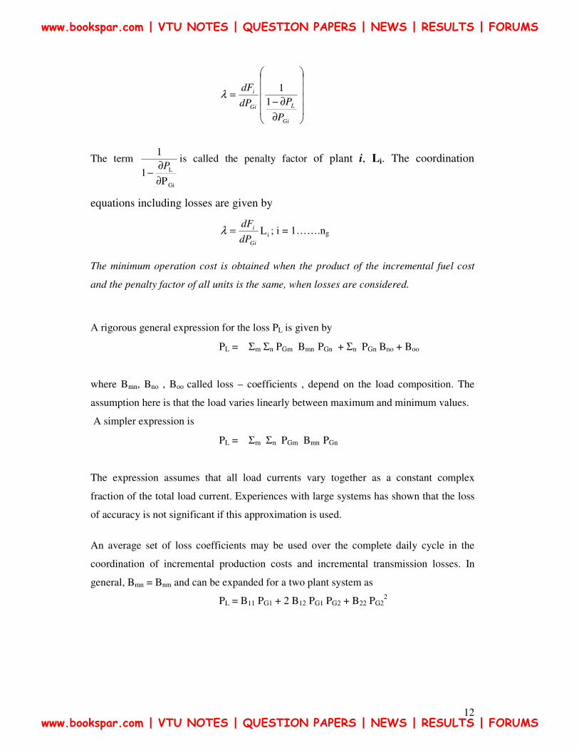
The term

Gi

L

P1

1

∂∂

−P

is called the penalty factor of plant i, Li. The coordination

equations including losses are given by

iLGi

i

dPdF

=λ ; i = 1…….ng

The minimum operation cost is obtained when the product of the incremental fuel cost

and the penalty factor of all units is the same, when losses are considered.

A rigorous general expression for the loss PL is given by

PL = Σm Σn PGm Bmn PGn + Σn PGn Bno + Boo

where Bmn, Bno , Boo called loss – coefficients , depend on the load composition. The

assumption here is that the load varies linearly between maximum and minimum values.

A simpler expression is

PL = Σm Σn PGm Bmn PGn

The expression assumes that all load currents vary together as a constant complex

fraction of the total load current. Experiences with large systems has shown that the loss

of accuracy is not significant if this approximation is used.

An average set of loss coefficients may be used over the complete daily cycle in the

coordination of incremental production costs and incremental transmission losses. In

general, Bmn = Bnm and can be expanded for a two plant system as

PL = B11 PG1 + 2 B12 PG1 PG2 + B22 PG22



13

Example 5

A generator is supplying a load. An incremental change in load of 4 MW requires

generation to be increased by 6 MW. The incremental cost at the plant bus is Rs 30 /

MWh. What is the incremental cost at the receiving end?

Solution:

1

1

GdPdF

= 30

Fig ; One line diagram of example 5

∆ PL = ∆ PG - ∆ PD = 2 MW

λ at receiving end is given by

4546

301

1 =×=∆∆

×=D

G

G PP

dPdFλ Rs / MWh

or 45

62

1

130

P1

1

G

L1

1 =−

×=

∆∆

−×=

PdPdF

G

λ Rs / MWh

Example 6

In a system with two plants, the incremental fuel costs are given by

2001.0 11

1 += GG

PdPdF

Rs / MWh

5.22015.0 22

2 += GG

PdPdF

Rs / MWh

The system is running under optimal schedule with PG1 = PG2 = 100 MW.

If G2

L

P∂∂P

= 0.2, find the plant penalty factors andG1

L

P∂∂P

.

Load

�PD = 4MW

�PL = 2MW

�PG = 6MW

301

1 =GdP

dF

G



14

Solution:

For economic schedule,

λ=iLGi

i

dPdF

;

Gi

Li

P1

1L

∂∂

−=

P;

For plant 2, PG2 = 100 MW

∴ ( ) .2.01

15.22100015.0 λ=

−+×

Solving, 30=λ Rs / MWh

L2 = 25.12.01

1 =−

λ=11

1 LdPdF

G

(0.01x100+20) L1 = 30

L1 = 1.428

L1 =

G1

L

P1

1

∂∂

−P

1.428 =

G1

L

P1

1

∂∂

−P

; Solving G1

L

P∂∂P

= 0.3

Example 7 A two bus system is shown in Fig. 8.8 If 100 MW is transmitted from plant 1 to the load,

a loss of 10 MW is incurred. System incremental cost is Rs 30 / MWh. Find PG1, PG2 and

power received by load if

0.1602.0 11

1 += GG

PdPdF

Rs / MWh

0.2004.0 22

2 += GG

PdPdF

Rs / MWh

G1 G2

Load

P G2PG1



15

Fig One line diagram of example 7

Solution;

Since the load is connected at bus 2 , no loss is incurred when plant two supplies the

load.

Therefore in (8.36) B12 = 0 and B22 = 0

2111L GPBP = ; 111

G1

L 2P GPBP

=∂∂

; 0.0PG2

L =∂∂P

From data we have PL = 10 MW, if PG1 = 100 MW

10 = B11 (100)2

B11 = 0.001 MW-1

Coordination equation with loss is

λλ =∂∂

+Gi

L

PP

dPdF

Gi

i

For plant 1 λλ =∂∂

+G1

L

1

1

PP

dPdF

G

(0.02 PG1 +16.0) + 30 (2 x 0.001 x PG1) = 30 0.08 PG1 = 30 - 16.0. From which, PG1 = 175 MW

For Plant 2 λλ =∂∂

+G2

L

1

2

PP

dPdF

G

0.04 PG2 + 20.0 = 30 or PG2 = 250 MW Loss = B11 PG1

2 = 0.001 x (175)2 = 30.625 MW PD = (PG1 + PG2) – PL = 394. 375 MW DERIVATION OF TRANSMISSION LOSS FORMULA An accurate method of obtaining general loss coefficients has been presented

by Kron. The method is elaborate and a simpler approach is possible by making the

following assumptions:

(i) All load currents have same phase angle with respect to a common reference

(ii) The ratio X / R is the same for all the network branches.



16

Consider the simple case of two generating plants connected to an arbitrary number of

loads through a transmission network as shown in Fig a

Fig Two plants connected to a number of loads through a transmission network Let’s assume that the total load is supplied by only generator 1 as shown in Fig 8.9b. Let

the current through a branch K in the network be IK1. We define

D

KK I

IN 1

1 =

It is to be noted that IG1 = ID in this case. Similarly with only plant 2 supplying the load

current ID, as shown in Fig 8.9c, we define

D

KK I

IN 2

2 =

(c)

ID IG2 = ID

IG1 = 0

1

2 IK2

(b)

ID

IG2 = 0

IG1 = ID

1

2 IK1

(a)

ID IG2

IG1

1

2 IK



17

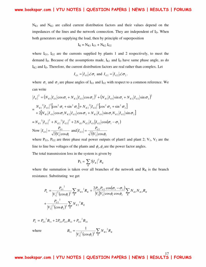
NK1 and NK2 are called current distribution factors and their values depend on the

impedances of the lines and the network connection. They are independent of ID. When

both generators are supplying the load, then by principle of superposition

IK = NK1 IG1 + NK2 IG2 where IG1, IG2 are the currents supplied by plants 1 and 2 respectively, to meet the

demand ID. Because of the assumptions made, IK1 and ID have same phase angle, as do

IK2 and ID. Therefore, the current distribution factors are real rather than complex. Let

111 σ∠= GG II and 222 σ∠= GG II .

where 1σ and 2σ are phase angles of IG1 and IG2 with respect to a common reference. We

can write

( ) ( )2222111

2222111

2 sinsincoscos σσσσ GKGKGKGKK ININININI +++=

= [ ] [ ]

[ ]222111222111

22

222

22

212

122

12

1

sinsincoscos2

sincossincos

σσσσσσσσ

GKGKGKGK

GKGK

ININININ

ININ

++

+++

= ( )2121212

22

22

12

1 cos2 σσ −++ GGKKGKGK IINNININ

Now 11

11

cos3 φV

PI G

G = and22

22

cos3 φV

PI G

G =

where PG1, PG2 are three phase real power outputs of plant1 and plant 2; V1, V2 are the

line to line bus voltages of the plants and 21 ,φφ are the power factor angles.

The total transmission loss in the system is given by

PL = KK

K RI2

3�

where the summation is taken over all branches of the network and RK is the branch

resistance. Substituting we get

( )( )

( ) KK

KG

KKK

KGG

KK

KG

RNV

P

RNNVVPP

RNV

PP

�

��

+

−+=

222

22

2

22

212121

2121212

12

1

21

L

cos

coscoscos2

cos

φ

φφσσ

φ

222

21221112

1L 2 BPBPPBPP GGGG ++=

where ( ) K

KK RN

VB �= 2

121

21

11cos

1

φ



18

( )

KKK

K RNNVV

B 212121

2112 coscos

cos�

−=

φφσσ

( ) K

KK RN

VB �= 2

222

22

22cos

1

φ

The loss – coefficients are called the B – coefficients and have unit MW-1.

For a general system with n plants the transmission loss is expressed as

( ) ( ) �� ++=K

KKn

nn

Gn

KK

G RNV

PN

V

PP 2

22

22

121

21

21

Lcos

........cos φφ

( )

Kk

KqKP

n

qpqp qpqp

qpGqGP RNNVV

PP��

≠=

−+

1, coscos

cos2

φφσσ

In a compact form

GqPq

n

p

n

qGp PBPP ��

= =

=1 1

L

( )�

−=

KKKqKP

qPqp

qpPq RNN

VVB

φφσσcoscos

cos

B – Coefficients can be treated as constants over the load cycle by computing them at

average operating conditions, without significant loss of accuracy.

Example 8 Calculate the loss coefficients in pu and MW-1

on a base of 50MVA for the network of

Fig below. Corresponding data is given below.

Ia = 1.2 – j 0.4 pu Za = 0.02 + j 0.08 pu

Ib = 0.4 - j 0.2 pu Zb = 0.08 + j 0.32 pu

Ic = 0.8 - j 0.1 pu Zc = 0.02 + j 0.08 pu

Id = 0.8 - j 0.2 pu Zd = 0.03 + j 0.12 pu

Ie = 1.2 - j 0.3 pu Ze = 0.03 + j 0.12 pu



19

Fig : Example 8

Solution: Total load current

IL = Id + Ie = 2.0 – j 0.5 = 2.061 ∠ -14.030A

IL1 = Id = 0.8 - j 0.2 = 0.8246 ∠ -14.030 A

;4.0IL

L1 =I

6.04.00.1IL

L2 =−=I

If generator 1, supplies the load then I1 = IL. The current distribution is shown in Fig a.

Fig a : Generator 1 supplying the total load

;0.1L

1 ==II

N aa ;6.0

L1 ==

II

N bb ;01 =CN ;4.01 =dN .6.01 =eN

Similarly the current distribution when only generator 2 supplies the load is shown in Fig b.

I2 = 0

c b a

Load 1 Load 2

0.6 IL 0.4 IL

IL IL 0.6 IL Ic = 0

G1 G2

d e

1

I2

c b a

Load 1 Load 2

Ie Id

I1

Ia Ib Ic

G1 G2

d e

Vref = 1.0 ∠ 00 2



20

Fig b: Generator 2 supplying the total load

Na2 =0; Nb2 = -0.4; Nc2 = 1.0; Nd2 = 0.4; Ne2 = 0.6

From Fig 8.10, V1 = Vref + ZaIa

= 1 ∠ 00 + (1.2 – j 0.4) (0.02 + j0.08)

= 1.06 ∠ 4.780 = 1.056 + j 0.088 pu.

V2 = Vref – Ib Zb + Ic Zc = 1.0 ∠ 00 – (0.4 – j 0.2) (0.08 + j 0.32) + (0.8 – j 0.1) (0.02 + j 0.08)

= 0.928 – j 0.05 = 0.93 ∠ -3.100 pu.

Current Phase angles

=1σ angle of I1(=Ia) = tan-1 043.182.14.0 −=��

��

� −

=2σ angle of ( ) 012 13.7

8.01.0

tan −=��

��

� −== −cII

( ) 98.0cos 21 =−σσ Power factor angles

92.0cos;21.2343.1878.4 100

1 ==+= φφ

998.0cos;03.410.313.7 2000

2 ==−= φφ

( ) ( ) ( )22

2222

21

21

21

11920.006.1

03.06.003.04.008.06.002.00.1

cos

×+×+×+×==�

φV

RNB K

KK

= 0.0677 pu

= 0.0677 x 2101354.0501 −×= MW-1

( )( )( ) KK

KK RNN

VVCos

B 212121

2112 coscos �

−=

φφσσ

IL

c b a

Load 1 Load 2

0.6 IL 0.4 IL

Ia = 0 0.4 IL IL

G1 G2

d e



21

= ( )( )( )( )[ ]03.06.06.003.04.04.008.06.04.092.0998.093.006.1

98.0 ××+××+××−

= - 0.00389 pu

= - 0.0078 x 10-2 MW-1

( )22

22

22

22cosφV

RNB K

KK�=

( )( ) ( )22

2222

998.093.0

03.06.003.04.002.00.108.04.0 ×+×+×+−=

= 0.056pu 210112.0 −×= MW-1



Documents

ECONOMIC OPERATION OF POWER SYSTEMS - …€¦ · 3 Fig .2 Heat rate curve. INCREMENTAL FUEL RATE CURVE The incremental fuel rate is equal to a small change in input divided by the