Back to BasicsBy Mark F. Milner, Chief Risk Officer, PMI Mortgage Insurance Co.

In This Issue

Economic and Real Estate Trends in the

Nation’s MSAs

The Value ofHomeownership

Looking Ahead

The Office of Federal Housing Enterprise Oversight (OFHEO) House Price

Index showed a year-over-year appreciation rate of 3.2 percent in the second

quarter – down from 4.45 percent in the first quarter and 9.98 percent a

year ago. Delinquency rates for home loans are surging, and you can’t turn

on the news without hearing stories about the real estate “crisis.”

PMI MORTGAGE INSURANCE CO.FALL 2007

�ECONOMICREAL ESTATE TRENDS

Real estate is cyclical – marked byperiods of solid appreciation, and

equally by periods of stagnation or decline.Cycles tend to be long, because realestate, for most people, is not a terriblyliquid investment. The rapidity of therecent changes in the real estate cyclemay be a surprise, but the fact that thingshave changed should not be. As with

changes in other asset cycles, we arereminded again that there is no new para-digm. After the dot com bust, the financialmarkets came back to the idea that funda-mentals matter for companies. Similarly,today we’re recognizing that when itcomes to the real estate market, the fun-damentals of lending have not changed.(continued on page 2)

SM

SM

MARK F. MILNER

Chief Risk OfficerPMI MORTGAGE INSURANCE CO.

LAVAUGHN M. HENRY, Ph.D.Director of Economic AnalysisPMI MORTGAGE INSURANCE CO.

OFHEO House Price Appreciation Rates

Geographic Distribution of Risk Scores

2

With that in mind, it’s a good time to consider what we can learnfrom this most recent cycle. At the top of the list, for me, are thefour Cs of good credit risk management.

Capital: First, some equity – even as little as 3 percent – helpseveryone. For lenders and investors, it’s a cushion that offerssome protection against the downside, which is important forthe long-term health of the loan. For borrowers, it’s an indicationof their commitment: they’ve thought about the step they’re taking,they’ve prepared for it, and they feel ready to own a home. Forthe mortgage finance system, it’s a stabilizing force that helpsensure long-term health. That’s not to say that 100 percentfinancing should never be made available – there are times whenit can be appropriate, under the right terms and conditions. Butlike other niche products, it should be matched with the group ofborrowers whose individual circumstances make it appropriate,and who are likely to be successful over the long term.

Capacity: For borrowers to be successful, and for lenders andother industry participants to thrive over the long term, home-ownership has to be sustainable. This means taking a hard lookat cash flow – verifying income, monthly cash flow, and the bor-rower’s ability to repay the loan. Low documentation loans,where income is stated but not verified, were developed as alegitimate solution for a small group of borrowers, and under theright terms and conditions there’s a place for them. They certainlycan streamline the underwriting process, but in many cases theborrower, the lender, and the investor will have a better foundationon which to build long term, sustainable homeownership with afully documented loan.

Character: A home purchase involves people – their hopes, theirdreams, their communities, and their families– to a much greaterdegree than any other investment. A positive character compo-nent in a credit transaction means a history of responsible creditbehavior. A home purchase transaction, and related mortgage, isthe largest financial transaction most people ever make. It

means taking on a large obligation, and to be successful, a borrower will need to manage his or her finances carefully. Aresponsible credit history is the best indicator we have ofwhether a borrower has demonstrated the willingness and abilityto manage their debt and if they are ready to shoulder the finan-cial obligations of homeownership.

Collateral: The valuation of a home is a critical part of the lendingdecision. Borrowers want to know they are paying a fair price fortheir homes. Lenders need an appraisal they trust to understandfully the risk they are taking. That makes an appraiser’s job espe-cially difficult in these times of slowing or declining home priceappreciation. In light of changing market conditions, appraisersshould consider carefully the factors that lead to a valuation. Thelender should review the appraisal thoroughly and, particularly insofter markets, use other sources to confirm the value, as well asconsider making adjustments to their loan or underwriting guide-lines. Overly aggressive appraisals can lead to transactions thatmay not be financially sound over the long term.

Careful underwriting is ultimately what ties these four Cs together.Experienced underwriting is required in order to review the loancharacteristics, balance the various factors involved, and deter-mine whether all the pieces fit the requested loan. Automatedsystems can help with this task, but they often can’t interpretnuances or identify potential problems the way an experiencedunderwriter can. Experienced, quality underwriting ensures thatthe borrower has the willingness and ability to repay the loan on aproperly valued home.

The real estate industry is endlessly innovative, which meansthat the next cycle won’t look exactly like this one. But thesebasic lessons – the four Cs of good credit management – willhold true tomorrow, as they have in the past. Sustainable home-ownership is everyone’s goal. Remembering the fundamentalsof credit can help us get there. �

Back to Basics(continued from page 1)

3

Economic and Real EstateTrends in the Nation’s MSAs

PMI’s U.S. Market Risk IndexSM ranks the likelihood of

home price declines in two years for the nation’s 381 met-

ropolitan statistical areas (MSAs). It is based on economic

factors including home price appreciation, volatility,

employment, and affordability.

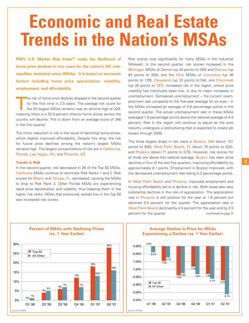
The risk of home price declines dropped in the second quarterfor the first time in 2.5 years. The average risk score forthe 50 largest MSAs remains near an all-time high at 329,

meaning there is a 32.9 percent chance home prices across thecountry will decline. This is down from an average score of 346in the first quarter.

The minor reduction in risk is the result of declining home prices,which slightly improved affordability. Despite this drop, the riskfor future price declines among the nation’s largest MSAsremains high. The largest concentrations of risk are in California,Florida, Las Vegas, NV, and Phoenix, AZ.

Trends in Risk

In the second quarter, risk decreased in 28 of the Top 50 MSAs.California MSAs continue to dominate Risk Ranks 1 and 2. Riskscores for Miami and Tampa, FL, decreased, causing the MSAsto drop to Risk Rank 3. Other Florida MSAs are experiencingrapid price deceleration and volatility, thus keeping them in thehigher risk ranks. MSAs that previously ranked low in the Top 50saw increased risk scores.

Risk scores rose significantly for many MSAs in the industrialMidwest. In the second quarter, risk scores increased in theMichigan MSAs of Detroit (up 44 points to 328) and Warren (up64 points to 300), and the Ohio MSAs of Columbus (up 36points to 129), Cleveland (up 33 points to154), and Cincinnati(up 30 points to 127). Increased risk in the region, where pricevolatility has historically been low, is due to major increases inunemployment. Demeaned unemployment – the current unem-ployment rate compared to the five-year average for an area – inthe MSAs increased an average of 0.6 percentage points in thesecond quarter. The actual unemployment rate in these MSAsaveraged 1.6 percentage points above the national average of 4.5percent. Risk in the region will continue to adjust as the autoindustry undergoes a restructuring that is expected to create joblosses through 2008.

The three largest drops in risk were in Boston, MA (down 101points to 400), West Palm Beach, FL (down 75 points to 532),and Phoenix (down 71 points to 575). However, risk scores forall three are above the national average. Boston has seen pricedeclines in four of the last five quarters, improving affordability byapproximately 8.1 points. Employment in Boston improved, withthe demeaned unemployment rate falling 0.3 percentage points.

In West Palm Beach and Phoenix, improved employment andhousing affordability led to a decline in risk. Both areas also sawsubstantial declines in the rate of appreciation. The appreciationrate in Phoenix is still positive for the year at 1.6 percent butdeclined 0.5 percent for the quarter. The appreciation rate inWest Palm Beach declined by 4.5 percent for the year and by 2.5percent for the quarter.

Percent of MSAs with Declining Prices

(vs. 1 Year Earlier)

Average Decline in Price for MSAs

Experiencing a Decline (vs. 1 Year Earlier)

(continued on page 9)

Source: OFHEO Source: OFHEO

4

The Big Picture

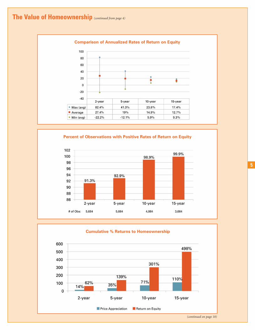
What we found was that, on a national level, owning a home for10 years remained a good way to build wealth and increase networth over the long term. Homeownership produced a positivereturn on investment 98.9 percent of the time. Over 15 years,that number increased to 99.9 percent. Individual rates of returnvaried across MSAs, but some common observations emergedfrom reviewing the data in its entirety.

Observation 1: The risk of loss drops the longer one owns a

home. With long-term ownership, the risk of loss is dispersedover a number of years, and the likelihood that one will receivea positive return increases.

Observation 2: The variation around the expected rate of

return on equity decreases the longer one owns a home. Therange of possible returns narrows as time passes, increasing thestability of the investment. The average annualized rate of returndecreases slightly over time but never dips below zero, even inmarkets with high price volatility.

Observation 3: If your goal is a predictable, positive return

on your investment, the timing of a home purchase is less

important than the length of time that you own your home.

The volatility around short-term investments is greater, meaningthat the potential for both gain and loss is higher if you invest forthe short term. The longer one holds the investment, the morestable the return will be. This result is found to be largely inde-pendent of when one purchases the property.

Up Close

When we took a regional look at three of the worst housing pricedeclines in the last 25 years, we found that in two instanceshome prices rebounded inside of 10 years, and that in oneinstance – the Texas oil patch crisis – home prices took nearly 15years to show a positive return.

In this period of slowing or declining home price appreciation, many new and prospective homeowners want to

know whether buying or owning a home now is a smart move. PMI wanted to address this concern on a national

and regional level so we looked at quarterly data for the 50 largest MSAs in OFHEO’s House Price Index from 1975

through the first quarter of 2007, and then took a closer look at three of the worst housing price declines over the

last 25 years.

To calculate the return on equity, we assumed that the average homeowner made a 20 percent down payment. We then

calculated the annualized rates of return on the initial equity investment at the 2-, 5-, 10- and 15-year marks.

(continued on page 10)

The Value of Homeownership

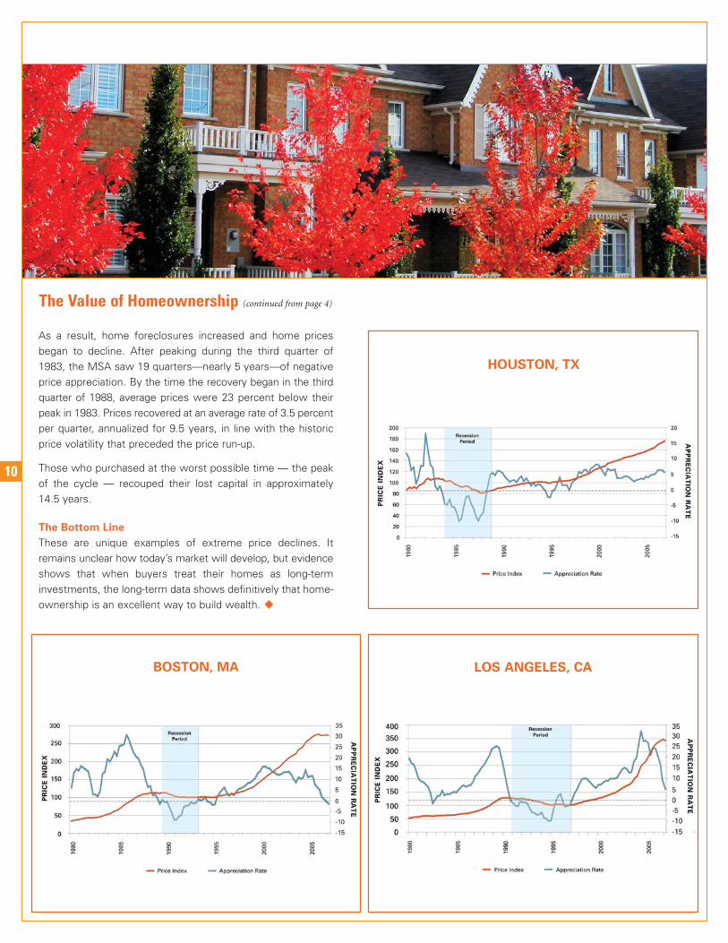
Los Angeles: 4th Qtr 1990 to 1st Qtr 1997

The end of the Cold War brought about a recession in the defense andtechnology industries in Southern California in 1990. The loss ofemployment reduced demand for homes, and foreclosures increasedthe supply of homes on the market.

Following years of double-digit price appreciation, price growthpeaked in the third quarter of 1990 and then turned negative for 24 ofthe following 26 quarters – 6.5 years. By the time the recovery beganin the second quarter of 1997, average prices were 21 percent belowtheir peak in 1990. Prices recovered at an average rate of 6.9 percentper quarter, annualized for the next 14 quarters.

Those who purchased at the worst possible time—the peak of thecycle—recouped their lost capital by the third quarter of 2000, 10years after the downturn began.

Boston: 4th Qtr 1989 to 1st Qtr 1993

The technology market in Boston expanded rapidly throughout the1980s and then stalled suddenly in 1989. The loss of jobs cost peopletheir homes and drove buyers out of the market.

After peaking during the third quarter of 1989, the MSA saw 14 quar-ters — 3.5 years — of negative price appreciation. By the time therecovery began in the second quarter of 1993, average prices were 7percent below their peak in 1989. After a false start at a recovery in1993, prices fell again for three quarters between the third quarter of1994 and first quarter of 1995. Price appreciation began in earnest inthe second quarter of 1995 at an average rate of 4.5 percent.

Those who purchased at the worst possible time — the peak of thecycle in 1989 — fully recouped their lost capital by the first quarter of1998, 8.5 years after the decline began.

Houston: 4th Qtr 1983 to 2nd Qtr 1988

In the early 1980s house prices in Houston appreciated rapidly as theoil industry boomed. In the mid-1980s oil prices dropped and domesticoil production ground to a halt. Houston was the epicenter of theindustry shakeup, which cost thousands of workers their jobs.

5

The Value of Homeownership (continued from page 4)

Comparison of Annualized Rates of Return on Equity

Percent of Observations with Positive Rates of Return on Equity

Cumulative % Returns to Homeownership

(continued on page 10)

MSA SCORE1

2ND QUARTER SM

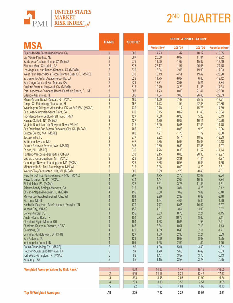
Riverside-San Bernardino-Ontario, CA 1 608 14.23 1.47 18.12 -16.65Las Vegas-Paradise, NV 2 587 20.58 -0.87 11.84 -12.72Santa Ana-Anaheim-Irvine, CA (MSAD) 2 579 11.50 -1.62 15.87 -17.49Phoenix-Mesa-Scottdale, AZ 2 575 22.17 1.57 26.05 -24.48Los Angeles-Long Beach-Glendale, CA (MSAD) 2 536 12.34 2.06 19.99 -17.93West Palm Beach-Boca Raton-Boynton Beach, FL (MSAD) 2 532 13.49 -4.51 19.47 -23.98Sacramento-Arden-Arcade-Roseville, CA 2 522 11.75 -6.07 6.05 -12.12San Diego-Carlsbad-San Marcos, CA 2 521 12.31 -3.63 5.21 -8.84Oakland-Fremont-Hayward, CA (MSAD) 2 516 10.79 -3.28 11.56 -14.84Fort Lauderdale-Pompano Beach-Deerfield Beach, FL (M 2 507 11.73 0.83 21.41 -20.58Orlando-Kissimmee, FL 2 506 17.04 3.63 26.46 -22.83Miami-Miami Beach-Kendall, FL (MSAD) 3 466 11.00 7.47 25.19 -17.71Tampa-St. Petersburg-Clearwater, FL 3 462 11.73 1.52 22.38 -20.86Washington-Arlington-Alexandria, DC-VA-MD-WV (MSAD) 3 439 10.78 1.17 15.76 -14.59San Jose-Sunnyvale-Santa Clara, CA 3 433 13.45 0.62 11.46 -10.84Providence-New Bedford-Fall River, RI-MA 3 427 7.69 -0.96 5.23 -6.19Nassau-Suffolk, NY (MSAD) 3 427 4.79 -0.09 10.11 -10.20Virginia Beach-Norfolk-Newport News, VA-NC 3 418 13.90 5.65 17.43 -11.78San Francisco-San Mateo-Redwood City, CA (MSAD) 3 405 9.81 -0.86 9.20 -10.06Boston-Quincy, MA (MSAD) 3 400 7.21 -1.78 1.72 -3.50Jacksonville, FL 3 377 9.22 5.14 18.53 -13.39Baltimore-Towson, MD 3 347 9.85 5.65 15.83 -10.18Seattle-Bellevue-Everett, WA (MSAD) 3 345 10.60 9.89 17.86 -7.97Edison, NJ (MSAD) 3 335 4.76 0.39 11.52 -11.14Portland-Vancouver-Beaverton, OR-WA 3 333 12.15 8.06 20.33 -12.27Detroit-Livonia-Dearborn, MI (MSAD) 3 328 4.00 -3.31 -1.44 -1.87Cambridge-Newton-Framingham, MA (MSAD) 3 323 5.56 -0.53 0.83 -1.36Minneapolis-St. Paul-Bloomington, MN-WI 3 313 3.86 0.69 4.20 -3.51Warren-Troy-Farmington Hills, MI (MSAD) 3 300 2.99 -2.78 -0.46 -2.31New York-White Plains-Wayne, NY-NJ (MSAD) 4 287 4.75 2.73 12.07 -9.34Newark-Union, NJ-PA (MSAD) 4 274 4.44 2.05 10.89 -8.84Philadelphia, PA (MSAD) 4 227 5.31 3.76 11.38 -7.61Atlanta-Sandy Springs-Marietta, GA 4 213 1.60 3.84 4.26 -0.42Chicago-Naperville-Joliet, IL (MSAD) 4 196 3.30 3.69 9.09 -5.40Milwaukee-Waukesha-West Allis, WI 4 191 3.90 2.98 6.08 -3.10St. Louis, MO-IL 4 184 1.94 4.02 5.32 -1.29Nashville-Davidson--Murfreesboro--Franklin, TN 4 179 4.77 6.65 10.02 -3.37Kansas City, MO-KS 4 159 1.31 3.64 3.06 0.57Denver-Aurora, CO 4 156 3.33 0.76 2.21 -1.45Austin-Round Rock, TX 4 154 5.73 10.76 8.65 2.11Cleveland-Elyria-Mentor, OH 4 154 1.88 -0.63 1.58 -2.21Charlotte-Gastonia-Concord, NC-SC 4 147 3.34 8.61 7.18 1.43Columbus, OH 4 129 1.39 0.40 2.11 -1.71Cincinnati-Middletown, OH-KY-IN 4 127 1.09 2.30 2.21 0.09San Antonio, TX 4 121 4.09 9.63 8.08 1.55Indianapolis-Carmel, IN 4 101 1.28 2.52 1.32 1.20Dallas-Plano-Irving, TX (MSAD) 5 95 1.88 5.01 3.49 1.52Houston-Sugar Land-Baytown, TX 5 94 1.78 5.66 6.49 -0.83Fort Worth-Arlington, TX (MSAD) 5 89 1.47 3.57 3.70 -0.13Pittsburgh, PA 5 85 1.15 3.53 3.28 0.25

Weighted Average Values by Risk Rank:8 1 608 14.23 1.47 18.12 -16.652 540 14.16 -0.25 17.42 -17.673 383 8.45 2.06 11.90 -9.844 203 3.38 3.58 7.57 -3.995 92 1.66 4.81 4.68 0.13

Top 50 Weighted Averages: All 329 7.32 2.37 10.97 -8.61

RANKPRICE APPRECIATION2

Volatility3 2Q ‘07 2Q ‘06 Acceleration4

2007UNEMPLOYMENT RATE

Rate6 Demeaned7

2Q ‘07 2Q ‘07 1Q ‘07

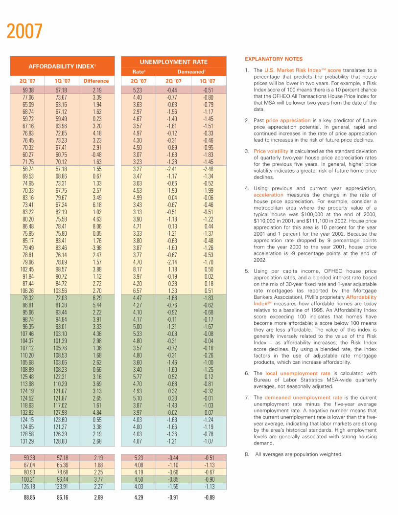
59.38 57.18 2.19 5.23 -0.44 -0.5177.06 73.67 3.39 4.40 -0.77 -0.8065.09 63.16 1.94 3.63 -0.63 -0.7968.74 67.12 1.62 2.97 -1.56 -1.1759.72 59.49 0.23 4.67 -1.40 -1.4567.16 63.96 3.20 3.57 -1.61 -1.5176.83 72.65 4.18 4.97 -0.12 -0.3376.45 73.23 3.23 4.30 -0.31 -0.4670.32 67.41 2.91 4.50 -0.89 -0.9560.27 60.75 -0.48 3.07 -1.68 -1.8371.75 70.12 1.63 3.23 -1.28 -1.4558.74 57.18 1.55 3.27 -2.41 -2.4869.53 68.86 0.67 3.47 -1.17 -1.3474.65 73.31 1.33 3.03 -0.66 -0.5270.33 67.75 2.57 4.53 -1.90 -1.9983.16 79.67 3.49 4.99 0.04 -0.0673.41 67.24 6.18 3.43 -0.67 -0.4683.22 82.19 1.02 3.13 -0.51 -0.5180.20 75.58 4.63 3.90 -1.18 -1.2286.48 78.41 8.06 4.71 0.13 0.4475.85 75.80 0.05 3.33 -1.21 -1.3785.17 83.41 1.76 3.80 -0.63 -0.4879.49 83.46 -3.98 3.87 -1.60 -1.2678.61 76.14 2.47 3.77 -0.67 -0.5379.66 78.09 1.57 4.70 -2.14 -1.70

102.45 98.57 3.88 8.17 1.18 0.5091.84 90.72 1.12 3.97 -0.19 0.0287.44 84.72 2.72 4.20 0.28 0.18

106.26 103.56 2.70 6.57 1.33 0.5178.32 72.03 6.29 4.47 -1.68 -1.8386.81 81.38 5.44 4.27 -0.76 -0.6295.66 93.44 2.22 4.10 -0.92 -0.6898.74 94.84 3.91 4.17 -0.11 -0.1796.35 93.01 3.33 5.00 -1.31 -1.67

107.46 103.10 4.36 5.33 -0.08 -0.08104.37 101.39 2.98 4.80 -0.31 -0.04107.12 105.76 1.36 3.57 -0.72 -0.16110.20 108.53 1.68 4.80 -0.31 -0.26105.68 103.06 2.62 3.60 -1.46 -1.00108.89 108.23 0.66 3.40 -1.60 -1.25125.48 122.31 3.16 5.77 0.52 0.12113.98 110.29 3.69 4.70 -0.68 -0.81124.19 121.07 3.13 4.93 0.32 -0.32124.52 121.87 2.65 5.10 0.33 -0.01118.63 117.02 1.61 3.87 -1.43 -1.03132.82 127.98 4.84 3.97 -0.02 0.07124.15 123.60 0.55 4.03 -1.68 -1.24124.65 121.27 3.38 4.00 -1.66 -1.19128.58 126.39 2.19 4.03 -1.36 -0.78131.29 128.60 2.68 4.07 -1.21 -1.07

59.38 57.18 2.19 5.23 -0.44 -0.5167.04 65.36 1.68 4.08 -1.10 -1.1380.93 78.68 2.25 4.19 -0.66 -0.67

100.21 96.44 3.77 4.50 -0.85 -0.90126.18 123.91 2.27 4.03 -1.55 -1.13

88.85 86.16 2.69 4.29 -0.91 -0.89

EXPLANATORY NOTES

1. The U.S. Market Risk IndexSM score translates to apercentage that predicts the probability that houseprices will be lower in two years. For example, a RiskIndex score of 100 means there is a 10 percent chancethat the OFHEO All Transactions House Price Index forthat MSA will be lower two years from the date of thedata.

2. Past price appreciation is a key predictor of futureprice appreciation potential. In general, rapid andcontinued increases in the rate of price appreciationlead to increases in the risk of future price declines.

3. Price volatility is calculated as the standard deviationof quarterly two-year house price appreciation ratesfor the previous five years. In general, higher pricevolatility indicates a greater risk of future home pricedeclines.

4. Using previous and current year appreciation,acceleration measures the change in the rate ofhouse price appreciation. For example, consider ametropolitan area where the property value of atypical house was $100,000 at the end of 2000,$110,000 in 2001, and $111,100 in 2002. House priceappreciation for this area is 10 percent for the year2001 and 1 percent for the year 2002. Because theappreciation rate dropped by 9 percentage pointsfrom the year 2000 to the year 2001, house priceacceleration is -9 percentage points at the end of2002.

5. Using per capita income, OFHEO house priceappreciation rates, and a blended interest rate basedon the mix of 30-year fixed rate and 1-year adjustablerate mortgages (as reported by the MortgageBankers Association), PMI’s proprietary AffordabilityIndexSM measures how affordable homes are todayrelative to a baseline of 1995. An Affordability Indexscore exceeding 100 indicates that homes havebecome more affordable; a score below 100 meansthey are less affordable. The value of this index isgenerally inversely related to the value of the RiskIndex – as affordability increases, the Risk Indexscore declines. By using a blended rate, the indexfactors in the use of adjustable rate mortgageproducts, which can increase affordability.

6. The local unemployment rate is calculated withBureau of Labor Statistics MSA-wide quarterlyaverages, not seasonally adjusted.

7. The demeaned unemployment rate is the currentunemployment rate minus the five-year averageunemployment rate. A negative number means thatthe current unemployment rate is lower than the five-year average, indicating that labor markets are strongby the area’s historical standards. High employmentlevels are generally associated with strong housingdemand.

8. All averages are population weighted.

AFFORDABILITY INDEX5

2Q ‘07 1Q ‘07 Difference

8

Mortgage Rates

Percent Change in Home Sales (from Prior Month)

Months Supply of Housing

Change in Employment Levels

Source: Freddie Mac

Source: National Association of Realtors - Existing, U.S. Census Bureau - New

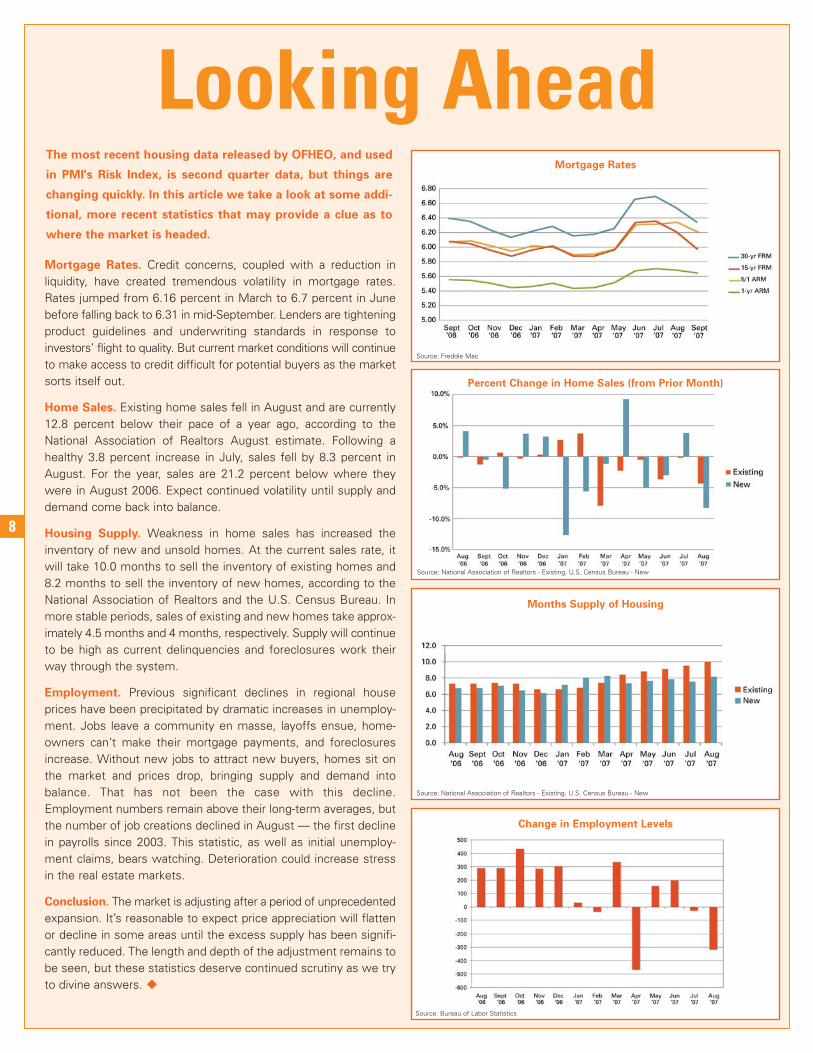
Looking AheadThe most recent housing data released by OFHEO, and used

in PMI's Risk Index, is second quarter data, but things are

changing quickly. In this article we take a look at some addi-

tional, more recent statistics that may provide a clue as to

where the market is headed.

Mortgage Rates. Credit concerns, coupled with a reduction in liquidity, have created tremendous volatility in mortgage rates.Rates jumped from 6.16 percent in March to 6.7 percent in Junebefore falling back to 6.31 in mid-September. Lenders are tighteningproduct guidelines and underwriting standards in response toinvestors’ flight to quality. But current market conditions will continueto make access to credit difficult for potential buyers as the marketsorts itself out.

Home Sales. Existing home sales fell in August and are currently12.8 percent below their pace of a year ago, according to theNational Association of Realtors August estimate. Following ahealthy 3.8 percent increase in July, sales fell by 8.3 percent inAugust. For the year, sales are 21.2 percent below where theywere in August 2006. Expect continued volatility until supply anddemand come back into balance.

Housing Supply. Weakness in home sales has increased theinventory of new and unsold homes. At the current sales rate, itwill take 10.0 months to sell the inventory of existing homes and8.2 months to sell the inventory of new homes, according to theNational Association of Realtors and the U.S. Census Bureau. Inmore stable periods, sales of existing and new homes take approx-imately 4.5 months and 4 months, respectively. Supply will continueto be high as current delinquencies and foreclosures work theirway through the system.

Employment. Previous significant declines in regional houseprices have been precipitated by dramatic increases in unemploy-ment. Jobs leave a community en masse, layoffs ensue, home-owners can’t make their mortgage payments, and foreclosuresincrease. Without new jobs to attract new buyers, homes sit onthe market and prices drop, bringing supply and demand into balance. That has not been the case with this decline.Employment numbers remain above their long-term averages, butthe number of job creations declined in August — the first declinein payrolls since 2003. This statistic, as well as initial unemploy-ment claims, bears watching. Deterioration could increase stressin the real estate markets.

Conclusion. The market is adjusting after a period of unprecedentedexpansion. It’s reasonable to expect price appreciation will flattenor decline in some areas until the excess supply has been signifi-cantly reduced. The length and depth of the adjustment remains tobe seen, but these statistics deserve continued scrutiny as we tryto divine answers. �

Source: National Association of Realtors - Existing, U.S. Census Bureau - New

Source: Bureau of Labor Statistics

9

Trends in the Nation’s MSAs (continued from page 3)

Trends in Home Price Appreciation

Since peaking in the second quarter of 2005, appreciation rateshave decelerated for seven of the last eight quarters, accordingto OFHEO. At the end of the second quarter, prices appreciatedat a year-over-year rate of 3.2 percent for conventional, conformingloans, a drop from the previous quarter’s year-over-year rate of4.5 percent.

The number of MSAs experiencing negative appreciation alsoincreased in the second quarter. Of the 381 MSAs tracked byOFHEO, 67 MSAs had negative year-over-year price appreciation.Of those that declined, the average decline was 2.9 percent.Among the 50 largest MSAs, 14 had negative year-over-yearappreciation rates, with an average decline of 2.21 percent. Ofthe remaining 331 MSAs, 53 experienced annual price declinesaveraging 3.12 percent.

For the first time in five quarters the percentage of MSAs expe-riencing price declines was higher for the Top 50 (28 percent)than for the remaining 331 MSAs (16 percent). This is a trendreversal that tells us the decline in home prices began to affectmore people in highly populated parts of the country whereprices and employment are typically more stable.

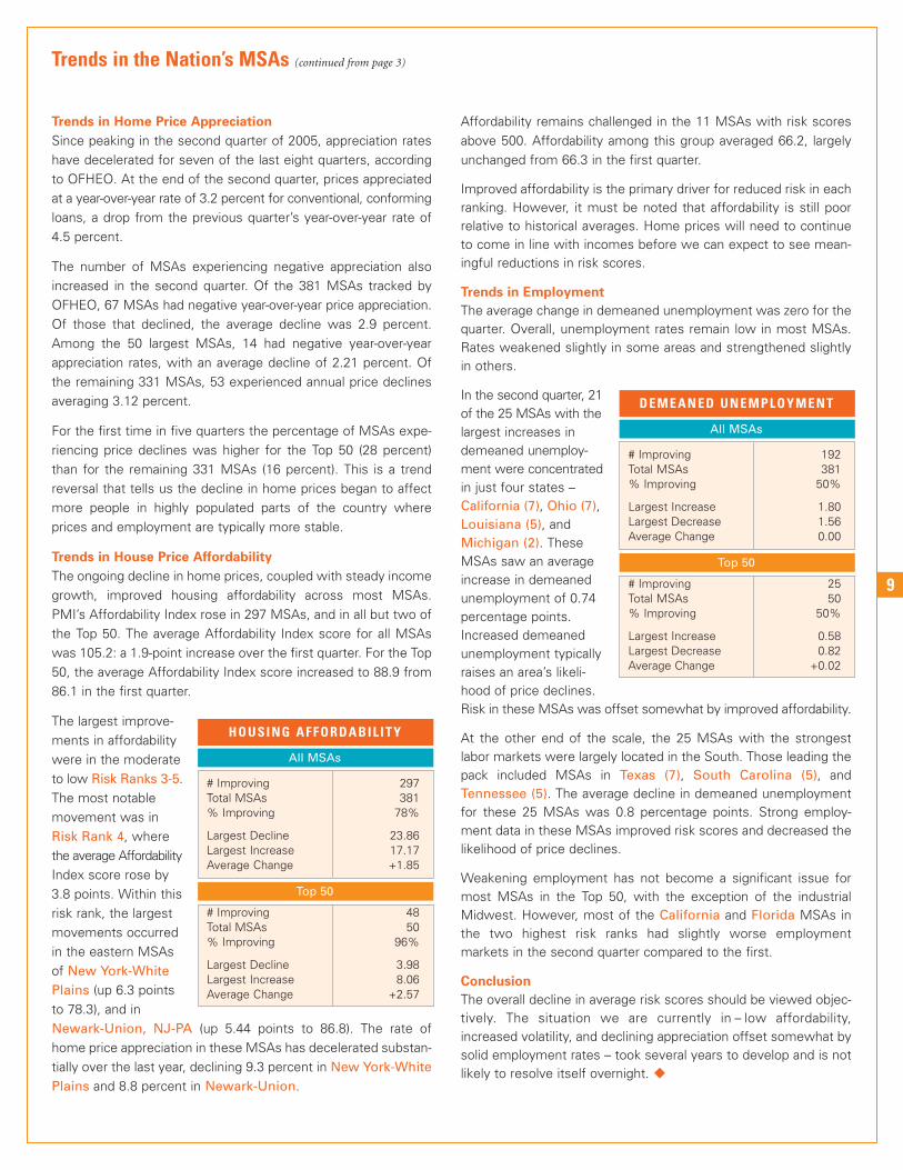
Trends in House Price Affordability

The ongoing decline in home prices, coupled with steady incomegrowth, improved housing affordability across most MSAs.PMI’s Affordability Index rose in 297 MSAs, and in all but two ofthe Top 50. The average Affordability Index score for all MSAswas 105.2: a 1.9-point increase over the first quarter. For the Top50, the average Affordability Index score increased to 88.9 from86.1 in the first quarter.

The largest improve-ments in affordabilitywere in the moderateto low Risk Ranks 3-5.The most notablemovement was inRisk Rank 4, wherethe average AffordabilityIndex score rose by3.8 points. Within thisrisk rank, the largestmovements occurredin the eastern MSAsof New York-WhitePlains (up 6.3 pointsto 78.3), and in Newark-Union, NJ-PA (up 5.44 points to 86.8). The rate ofhome price appreciation in these MSAs has decelerated substan-tially over the last year, declining 9.3 percent in New York-WhitePlains and 8.8 percent in Newark-Union.

Affordability remains challenged in the 11 MSAs with risk scoresabove 500. Affordability among this group averaged 66.2, largelyunchanged from 66.3 in the first quarter.

Improved affordability is the primary driver for reduced risk in eachranking. However, it must be noted that affordability is still poor relative to historical averages. Home prices will need to continueto come in line with incomes before we can expect to see mean-ingful reductions in risk scores.

Trends in Employment

The average change in demeaned unemployment was zero for thequarter. Overall, unemployment rates remain low in most MSAs.Rates weakened slightly in some areas and strengthened slightlyin others.

In the second quarter, 21of the 25 MSAs with thelargest increases indemeaned unemploy-ment were concentratedin just four states –California (7), Ohio (7),Louisiana (5), andMichigan (2). TheseMSAs saw an averageincrease in demeanedunemployment of 0.74percentage points.Increased demeanedunemployment typicallyraises an area’s likeli-hood of price declines. Risk in these MSAs was offset somewhat by improved affordability.

At the other end of the scale, the 25 MSAs with the strongestlabor markets were largely located in the South. Those leading thepack included MSAs in Texas (7), South Carolina (5), andTennessee (5). The average decline in demeaned unemploymentfor these 25 MSAs was 0.8 percentage points. Strong employ-ment data in these MSAs improved risk scores and decreased thelikelihood of price declines.

Weakening employment has not become a significant issue formost MSAs in the Top 50, with the exception of the industrialMidwest. However, most of the California and Florida MSAs inthe two highest risk ranks had slightly worse employment markets in the second quarter compared to the first.

Conclusion

The overall decline in average risk scores should be viewed objec-tively. The situation we are currently in – low affordability,increased volatility, and declining appreciation offset somewhat bysolid employment rates – took several years to develop and is notlikely to resolve itself overnight. �

HOUSING AFFORDABIL ITY

All MSAs

# Improving 297Total MSAs 381% Improving 78%

Largest Decline 23.86Largest Increase 17.17Average Change +1.85

Top 50

# Improving 48Total MSAs 50% Improving 96%

Largest Decline 3.98Largest Increase 8.06Average Change +2.57

DEMEANED UNEMPLOYMENT

All MSAs

# Improving 192Total MSAs 381% Improving 50%

Largest Increase 1.80Largest Decrease 1.56Average Change 0.00

Top 50

# Improving 25Total MSAs 50% Improving 50%

Largest Increase 0.58Largest Decrease 0.82Average Change +0.02

10

The Value of Homeownership (continued from page 4)

As a result, home foreclosures increased and home pricesbegan to decline. After peaking during the third quarter of1983, the MSA saw 19 quarters—nearly 5 years—of negativeprice appreciation. By the time the recovery began in the thirdquarter of 1988, average prices were 23 percent below theirpeak in 1983. Prices recovered at an average rate of 3.5 percentper quarter, annualized for 9.5 years, in line with the historicprice volatility that preceded the price run-up.

Those who purchased at the worst possible time — the peakof the cycle — recouped their lost capital in approximately14.5 years.

The Bottom Line

These are unique examples of extreme price declines. Itremains unclear how today’s market will develop, but evidenceshows that when buyers treat their homes as long-terminvestments, the long-term data shows definitively that home-ownership is an excellent way to build wealth. �

HOUSTON, TX

LOS ANGELES, CABOSTON, MA

11

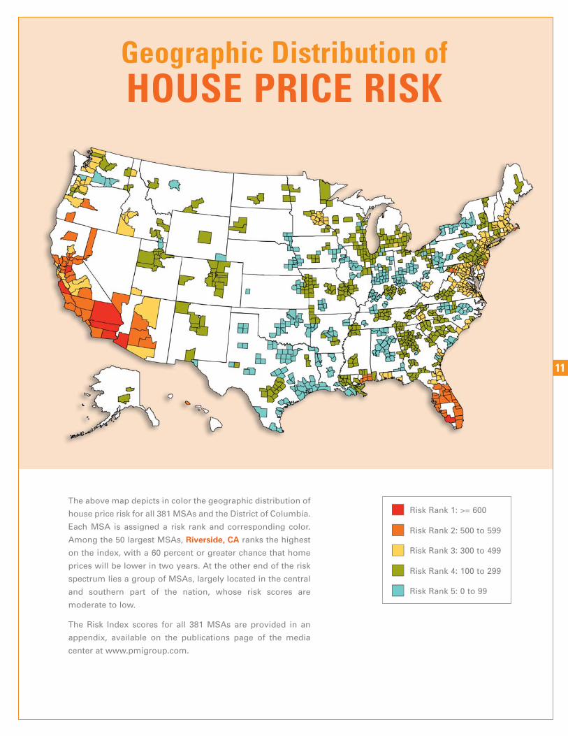
Geographic Distribution ofHOUSE PRICE RISK

Risk Rank 1: >= 600

Risk Rank 2: 500 to 599

Risk Rank 3: 300 to 499

Risk Rank 4: 100 to 299

Risk Rank 5: 0 to 99

The above map depicts in color the geographic distribution of

house price risk for all 381 MSAs and the District of Columbia.

Each MSA is assigned a risk rank and corresponding color.

Among the 50 largest MSAs, Riverside, CA ranks the highest

on the index, with a 60 percent or greater chance that home

prices will be lower in two years. At the other end of the risk

spectrum lies a group of MSAs, largely located in the central

and southern part of the nation, whose risk scores are

moderate to low.

The Risk Index scores for all 381 MSAs are provided in an

appendix, available on the publications page of the media

center at www.pmigroup.com.

800.966.4PMI (4764)

www.pmi-us.com

PMI 2

05 (1

0.07

)

07-0470

Please contact your PMI representativefor more information or printed versions.

The ERET report is produced quarterly.

You can download a PDF version online:http://www.pmi-us.com

METROPOLITAN AREA ECONOMICINDICATORS STATISTICAL MODEL OVERVIEW

The U.S. Market Risk Index is based on the results of

applying a statistical model to data on local economic

conditions, income, and interest rates, as well as

judgmental adjustments in order to reflect information

that goes beyond the Risk Index’s quantitative scope. For

each Metropolitan Statistical Area (MSA) or Metropolitan

Statistical Area Division (MSAD), the statistical model

estimates the probability that an index of metropolitan-

area-wide home prices will be lower in two years, with an

index value of 100 implying a 10% probability of falling

house prices.

Home prices are measured with a Repeat Sales Index

provided by the Office of Federal Housing Enterprise

Oversight (OFHEO). This method follows homes that are

sold repeatedly over the observation period and uses the

change in the purchase prices to construct a price index.

The index is based on data from Fannie Mae and Freddie

Mac and covers only homes financed with loans securitized

by these two companies. Consequently, this index does not

apply to high-end properties requiring jumbo loans.

Periodically, we may re-estimate our model to update the

statistical parameters with the latest available data. We

also may make adjustments from time to time to account

for general macroeconomic developments that are not

captured by our model.

Cautionary Statement: Statements in this document that are not historical facts or that relate to future plans, events or performance are ‘forward-looking’ statements within the

meaning of the Private Securities Litigation Reform Act of 1995. These forward-looking statements include, but are not limited to, PMI’s U.S. Market Risk Index and any related discussion,

and statements relating to future economic and housing market conditions. Forward-looking statements are subject to a number of risks and uncertainties including, but not limited to,

the following factors: changes in economic conditions, economic recession or slowdowns, adverse changes in consumer confidence, declining housing values, higher unemployment,

deteriorating borrower credit, changes in interest rates, the effects of natural disasters, or a combination of these factors. Readers are cautioned that any statements with respect to

future economic and housing market conditions are based upon current economic conditions and, therefore, are inherently uncertain and highly subject to changes in the factors

enumerated above. Other risk and uncertainties are discussed in the Company’s filings with the Securities and Exchange Commission, including our report on Form 10-K for the year ended

December 31, 2006 and Form 10-Q for the quarter ended June 30, 2007.

© 2007 PMI Mortgage Insurance Co.