Embed Size (px)
Citation preview
Hyd
rolo
gic
al S
ervi
ce M
ap
pin
g
Economic Valuation of Changes in the Amazon Forest Area
www.csr.ufmg.br/amazones
2017 Research Group on Atmosphere-Biosphere Interaction, Universidade Federal de Viçosa
Economic Valuation of Changes
in the Amazon Forest Area
Hydrological Service Mapping
Authors:
Marcos Heil Costa Gabrielle Ferreira Pires Vitor Cunha Fontes Fernando Martins Pimenta Livia Maria Brumatti de Souza Matheus Lucas da Silva
Publisher: Centro de Sensoriamento Remoto/Universidade Federal de Minas Gerais
Belo Horizonte
2017
3
© 2017 Centro de Sensoriamento Remoto, Universidade Federal de Minas
Gerais
Research Group on Atmosphere-Biosphere Interaction, UFV
www.biosfera.dea.ufv.br / +55 31 3899-1899 / [email protected]
Costa, Marcos Heil.
Economic Valuation of Changes in the Amazon Forest Area:
Hidrological Service Mapping / Marcos Heil Costa, Gabrielle Ferreira Pires,
Vitor Cunha Fontes, Fernando Martins Pimenta, Livia Maria Brumatti de
Souza, Matheus Lucas da Silva. 1. ed. - Belo Horizonte: Ed. IGC/UFMG,
2017. 38 p.
Include references.
ISBN: 978-85-61968-08-3
1. Amazon rainforest. 2. Economic activities. 3. Rainfall dynamics
Publisher: Centro de Sensoriamento Remoto/UFMG
Av. Antônio Carlos, 6.627 - Instituto de Geociências - Pampulha - CEP: 31270-
901, Belo Horizonte - MG, Brazil.
4
Index
1. Introduction .................................................................................................................. 5
2. Calculation of source and destination of water vapor precipitated and evaporated in
Amazonia, for different levels of Amazon forest cover ....................................................... 6
2.1. Data used and description of the scenarios of deforestation ...................................................... 6
2.2. Validation of the simulated climatology of precipitation patterns in South America..................7
2.3. Theory to compute the simulated source and destination of water vapor.................................. 8
2.4. Source of water vapor .................................................................................................................10
3. Revenue of the main economic activities that depend on climate and change due to
deforestation .................................................................................................................. 15
3.1. Soybeans .....................................................................................................................................17
3.1.1. Calculation .......................................................................................................................... 17
3.1.2. Results ................................................................................................................................. 19
3.2. Cattle beef ...................................................................................................................................22
3.2.1. Calculation .......................................................................................................................... 22
3.2.2. Results ................................................................................................................................. 24
3.3. Hydropower ................................................................................................................................26
3.3.1. Calculation .......................................................................................................................... 26
3.3.2. Results ................................................................................................................................. 27
3.4. Statistical significance of the results ...........................................................................................28
4. Estimation of the climate regulation service provided by the Amazon .......................... 29
4.1. Calculation ..................................................................................................................................29
4.2. Results .........................................................................................................................................30
5. Online Platforms .......................................................................................................... 34
6. Final Remarks .............................................................................................................. 37
7. References ................................................................................................................... 38
5
1. Introduction
This is the fourth deliverable of Output Category 2 of the project ‘Economic Valuation
of Changes in Amazon Forest Area’, executed by FUNARBE and UFV. At this point nearly all of
the results of this Output are complete, including new significance analyses of the results, and
the work integrating the hydrological analysis with the valuation platform. A manuscript
detailing the calculations of the climate regulation ecosystem service provided by the Amazon
rainforest is also completed, and is ready for submission to Environmental Research Letters.
At this point the only activities pending are the final training/outreach session and a summary
scientific paper, joint with the core team.
This report summarizes all of the work conducted by the FUNARBE/UFV team concerning the
Amazon Hydrological Service Mapping from the beginning of the project to its conclusion. The
report is divided in four Chapters. The results found in Chapters 2 and 3 have already
presented in previous reports (Deliverables 2 and 3, respectively). New results, not previously
presented, are found in Chapters 4 and 5.
Chapter 2 describes the work completed about the calculation of the sources and destination
of water vapor precipitated and evaporated in Amazonia, for different levels of Amazon forest
cover, presented in the Deliverable 2 document. Chapter 3 describes the calculations of the
effects of changes in climate (mainly rainfall, but also other climate variables) on the three
main economic activities in Amazonia that depend on climate: soybean production, cattle
beef production and hydropower generation, and the change in revenue due to climate
change, presented in the Deliverable 3 document. Chapter 4 presents new results on the
estimation of the climate regulation service provided by the Amazon Rainforest. Finally,
Chapter 5 describes the work done on the Deforestation and Rainfall platform, as well as on
the Amazon Rainforest Evaluation Platform.
6
2. Calculation of source and destination of water vapor
precipitated and evaporated in Amazonia, for different
levels of Amazon forest cover
2.1. Data used and description of the scenarios of deforestation
As previously specified in the project, the contribution of any given forest pixel for the
regional climate should be calculated. The role of each individual pixel for local climate is
small, and as pixels are aggregated, due to the non-linear nature of the climate system, they
usually are added non-linearly. A simulation of all the possible combination of deforested
pixels in Amazonia would require millions of climate simulations and would be impossible to
perform. The alternative used, which considerably simplifies the problem and follows a
plausible and realistic deforestation trajectory, is through the analyses of deforestation
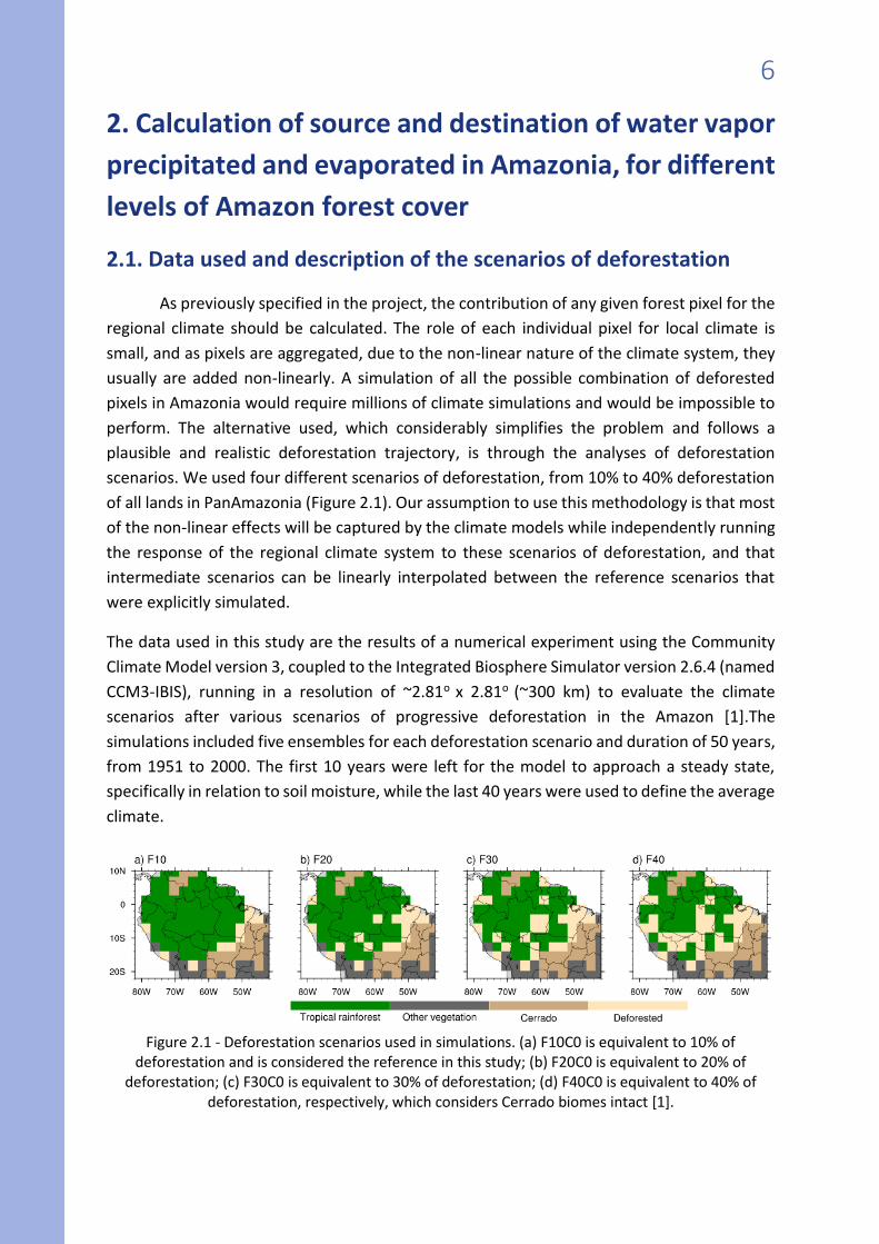
scenarios. We used four different scenarios of deforestation, from 10% to 40% deforestation
of all lands in PanAmazonia (Figure 2.1). Our assumption to use this methodology is that most
of the non-linear effects will be captured by the climate models while independently running
the response of the regional climate system to these scenarios of deforestation, and that
intermediate scenarios can be linearly interpolated between the reference scenarios that
were explicitly simulated.
The data used in this study are the results of a numerical experiment using the Community
Climate Model version 3, coupled to the Integrated Biosphere Simulator version 2.6.4 (named
CCM3-IBIS), running in a resolution of ~2.81o x 2.81o (~300 km) to evaluate the climate
scenarios after various scenarios of progressive deforestation in the Amazon [1].The
simulations included five ensembles for each deforestation scenario and duration of 50 years,
from 1951 to 2000. The first 10 years were left for the model to approach a steady state,
specifically in relation to soil moisture, while the last 40 years were used to define the average
climate.
Figure 2.1 - Deforestation scenarios used in simulations. (a) F10C0 is equivalent to 10% of
deforestation and is considered the reference in this study; (b) F20C0 is equivalent to 20% of deforestation; (c) F30C0 is equivalent to 30% of deforestation; (d) F40C0 is equivalent to 40% of
deforestation, respectively, which considers Cerrado biomes intact [1].
7
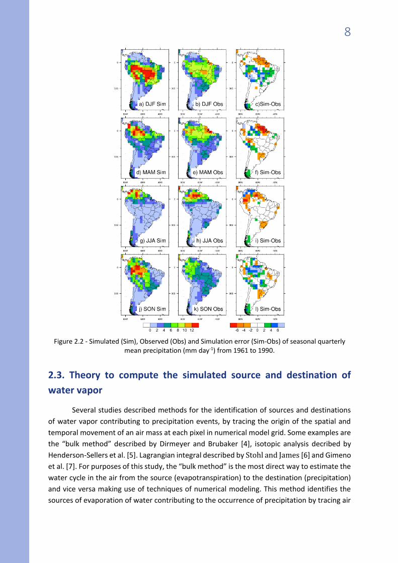
2.2. Validation of the simulated climatology of precipitation patterns
in South America
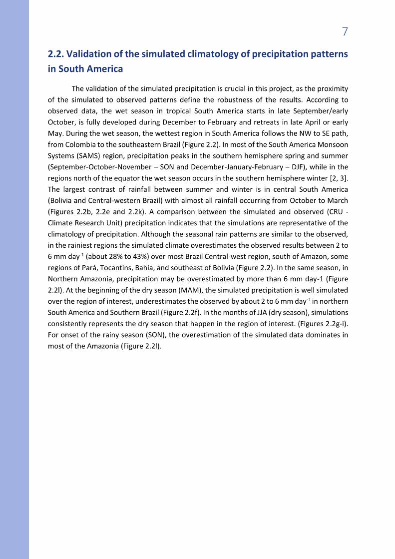
The validation of the simulated precipitation is crucial in this project, as the proximity
of the simulated to observed patterns define the robustness of the results. According to
observed data, the wet season in tropical South America starts in late September/early
October, is fully developed during December to February and retreats in late April or early
May. During the wet season, the wettest region in South America follows the NW to SE path,
from Colombia to the southeastern Brazil (Figure 2.2). In most of the South America Monsoon
Systems (SAMS) region, precipitation peaks in the southern hemisphere spring and summer
(September-October-November – SON and December-January-February – DJF), while in the
regions north of the equator the wet season occurs in the southern hemisphere winter [2, 3].
The largest contrast of rainfall between summer and winter is in central South America
(Bolivia and Central-western Brazil) with almost all rainfall occurring from October to March
(Figures 2.2b, 2.2e and 2.2k). A comparison between the simulated and observed (CRU -
Climate Research Unit) precipitation indicates that the simulations are representative of the
climatology of precipitation. Although the seasonal rain patterns are similar to the observed,
in the rainiest regions the simulated climate overestimates the observed results between 2 to
6 mm day-1 (about 28% to 43%) over most Brazil Central-west region, south of Amazon, some
regions of Pará, Tocantins, Bahia, and southeast of Bolivia (Figure 2.2). In the same season, in
Northern Amazonia, precipitation may be overestimated by more than 6 mm day-1 (Figure
2.2l). At the beginning of the dry season (MAM), the simulated precipitation is well simulated
over the region of interest, underestimates the observed by about 2 to 6 mm day-1 in northern
South America and Southern Brazil (Figure 2.2f). In the months of JJA (dry season), simulations
consistently represents the dry season that happen in the region of interest. (Figures 2.2g-i).
For onset of the rainy season (SON), the overestimation of the simulated data dominates in
most of the Amazonia (Figure 2.2l).
8
Figure 2.2 - Simulated (Sim), Observed (Obs) and Simulation error (Sim-Obs) of seasonal quarterly
mean precipitation (mm day-1) from 1961 to 1990.
2.3. Theory to compute the simulated source and destination of
water vapor
Several studies described methods for the identification of sources and destinations
of water vapor contributing to precipitation events, by tracing the origin of the spatial and
temporal movement of an air mass at each pixel in numerical model grid. Some examples are
the “bulk method” described by Dirmeyer and Brubaker [4], isotopic analysis decribed by
Henderson-Sellers et al. [5]. Lagrangian integral described by Stohl and James [6] and Gimeno
et al. [7]. For purposes of this study, the “bulk method” is the most direct way to estimate the
water cycle in the air from the source (evapotranspiration) to the destination (precipitation)
and vice versa making use of techniques of numerical modeling. This method identifies the
sources of evaporation of water contributing to the occurrence of precipitation by tracing air
9
flow backwards and / or forwards in time through the analysis of numerical grid model data.
The method is based on the use of two-dimensional data of precipitation and
evapotranspiration, and three-dimensional data of wind and water vapor and can be applied
to field data or data generated by a climate model. Ideally, data should be of high temporal-
resolution (hourly or less), however monthly fields can be used if the covariance terms are
available. This method assumes that:
every molecule of water vapor within the tropospheric column is equally likely to
precipitate;
the water evaporated from the surface mixes uniformly through the atmospheric column
and does not precipitate in the same pixel (the latter assumption may incur in an error
from 1.2 to 3.7% according to Dirmeyer and Brubaker [4];
the water vapor portion may fall from any level and can be back to a random level.
From the conservation of water vapor:
PEy
F
x
F vu
eq. (1)
Where Fu and Fv are the horizontal water vapor fluxes in the zonal and meridional directions
respectively, E is the evapotranspiration and P is the precipitation. The water vapor flux
integrated in the whole atmospheric column of each pixel is given by the following
expressions:
dpuqg
wF
ps
p
u
u 0
, where ´´q quuuq eq. (2)
dpvqg
wF
ps
p
v
v 0
, where ´´q qvvvq eq. (3)
u , v , q , ´´qv , ´´qu are the zonal and meridional mean wind speed, mean specific humidity and
their covariance, respectively [8]. wu and wv are the horizontal widths perpendicular to the
directions of the zonal and meridional moisture flux respectively, g is the acceleration due to
gravity (equal to 9.80616 m.s-2) and ps is the surface pressure. Isolating the precipitation P in
the water balance equation 1 we have:
y
F
x
FEP vu
eq. (4)
From equation 4 we could calculate the moisture proportions corresponding to each
contributing factor. The average flux of the neighbor pixels result in an average flux at the
interface of the pixel in question, which can be positive or negative, and by logical analysis
was the input or output of each grid pixel, thereby determining the sources and destinations
10
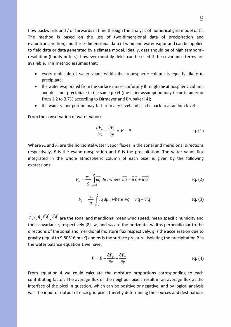
of precipitated and evaporated water vapor in the study region. From the 84 pixels of the
Amazon in our model, 8 deforestation scenarios and monthly average of water vapor flow in
40 years, 8,064 maps (84 × 8 × 12) were generated for South America. However, for purposes
of demonstration of the results, in this report we show only maps of source of water vapor to
the Mato Grosso state soybean productive region and to Xingu and Madeira basins (Figure
2.3). These regions were chosen mainly because they are located in or nearly recently
deforested areas and hold important economic activities that rely on rainfall, as hydropower
and agriculture.
Figure 2.3 - Orientation map showing the soybean area in Mato Grosso and the Madeira and Xingu
basins with potential for hydropower generation.
2.4. Source of water vapor
Here, our analysis is concentrated in the two quarters SON and DJF, when soybean
crops develop. SON are also the most critical months of expected change in the hydropower
generation. In the case of all three dams analyzed, the lakes formed are relatively small, and
insufficient to keep the hydropower plant running at maximum capacity during the dry
season. From previous studies using the same model [9] we expect a late onset of the rainy
season during the SON trimester, thus making the analysis of this period critical under
deforestation conditions.
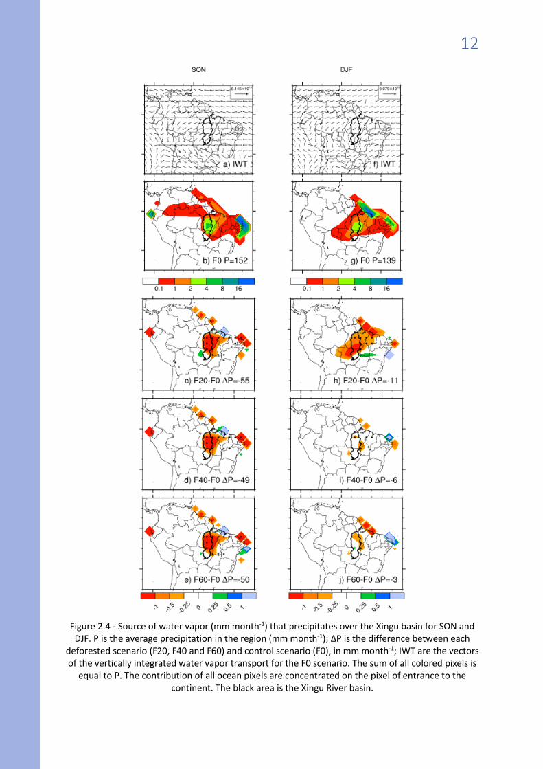
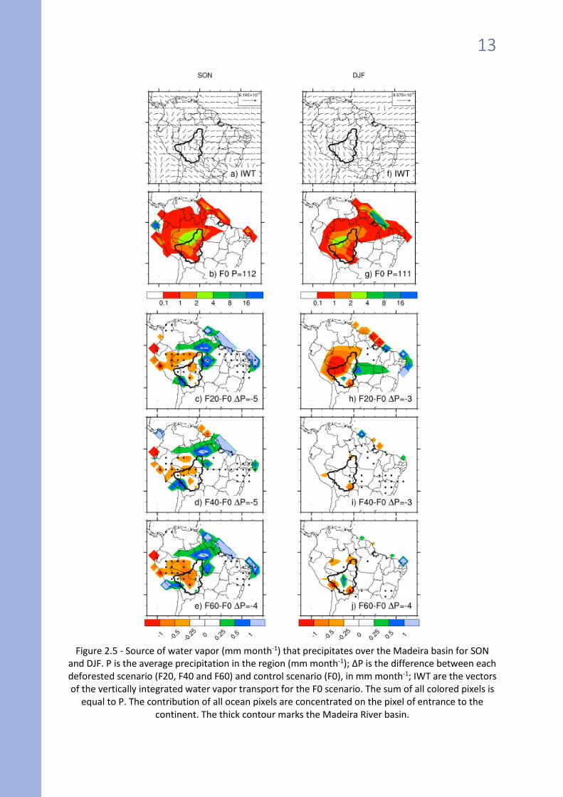
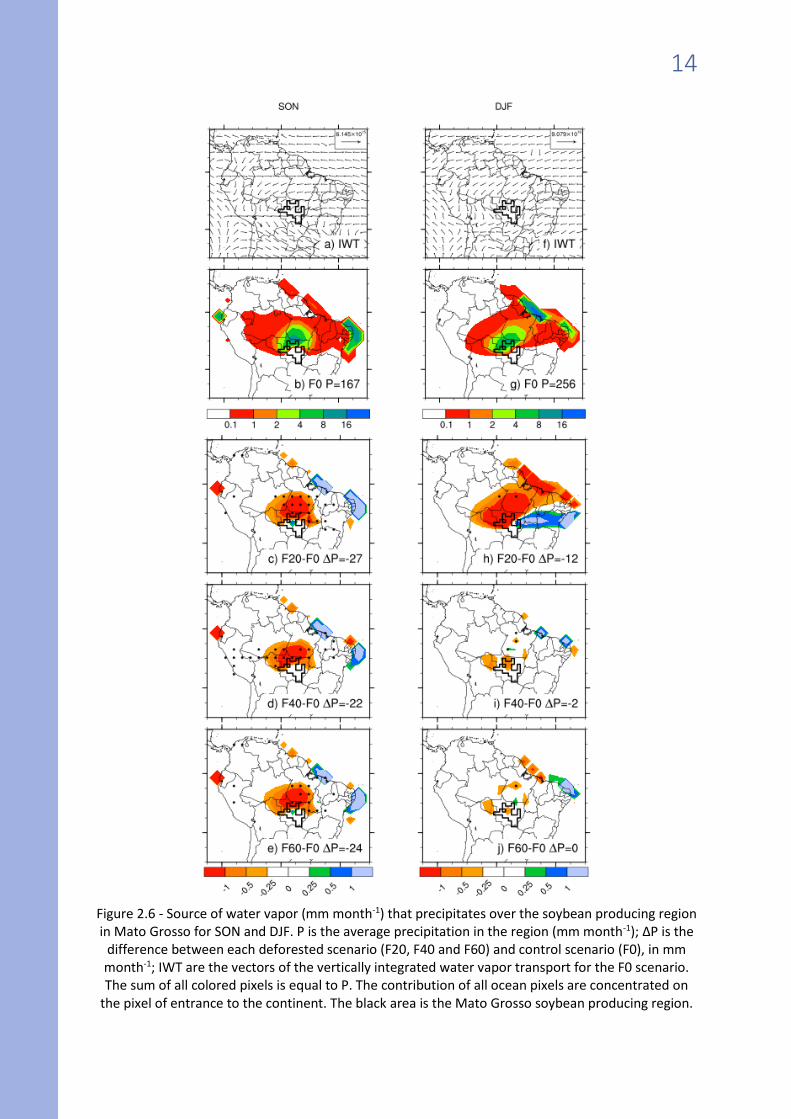
Figures 2.4, 2.5 and 2.6 show the vertically integrated water vapor transport for the F0
scenario, and the source of water vapor that precipitates on the Xingu, Madeira and soybean
producing regions, respectively, for the scenario F0, and anomalies for the scenarios F20, F40
and F60. In these figures, the sum of all pixels in the map is equal to the amount of
precipitation inside the basin.
11
The Xingu basin is relatively close to the ocean, which indicates that most of the water vapor
that precipitates inside the basin was evaporated from the Atlantic Ocean (Figures 2.4b and
2.4g). During SON, the wind and water vapor transport is typically easterly (Figure 2.4a), while
in DJF it is typically from Northeast (Figure 2.4f). However, in both cases, the air passes over
highly deforested land. Actually, most of deforestation on the 20% scenario happens upwind
of the Xingu basin (Figure 2.1). Consequently, the deforested regions contribute less water
vapor to the precipitation over the Xingu basin (Figures 2.4c and 2.4h). From the circulation
patterns, the additional deforestation in the F40 and F60 scenarios do not cause additional
reduction in rainfall over the Xingu basin (Figures 2.4d, 2.4e, 2.4i and 2.4j), as it happens
mostly downwind of the basin.
The Madeira basin is a large region located inland, on the southwest of the Amazon basin, and
relatively close to the Andes (Figure 2.5). Contrary to the Xingu basin, the humid air crosses a
large portion of the continent before precipitating on the Madeira basin (Figure 2.5a and 2.5f).
In SON, most of water vapor that precipitates in the basin has evaporated either inside it or
nearby (Figure 2.5b), while during DJF, the contribution from the Atlantic Ocean is larger. Most
importantly, the main air trajectory, mostly parallel to the equator and turning to SE before
arriving at the Madeira basin, crosses a region with little deforestation in all scenarios
analyzed. For all three deforestation levels and both seasons analyzed, reductions in rainfall
are in the range of 3-5 mm/month, or about 4%.
The soybean-producing region in Mato Grosso is to the south and to the west of the Xingu
River basin, and between the two other basins analyzed (Figure 2.3). Because of this
intermediary geographical position, the air trajectory to the region has elements from the two
previous cases. In SON, air comes mainly from the east, and turns to SW before entering the
soybean area (Figure 2.6a), and most of the water vapor that precipitates on this region has
evaporated either nearby or on the ocean. Decreases in P for the three deforested scenarios
are in the range of 22 to 27 mm/month (13-16%). Most of the decreases in the source of water
vapor that contributes to the precipitation over the region is from nearby pixels (Figures 2.6c-
2.6e). In scenario F20, half of these main contributing pixels are deforested and the other half
are still forested (Figure 2.1), but the fraction of deforested pixels increase proportionally in
the F40 and F60 scenarios. During DJF in the scenario F20, air comes mainly from northeast
and east, and crosses heavily deforested regions to the NE of the region. During this season,
the source of water vapor shifts, decreasing from the pixels NE of the region, but increasing
to the E of the region (Figure 2.6h), and the total change in rainfall is -12 mm/month (~5%).
For higher deforestation scenarios (F40 and F60), apparently competing mechanisms set in,
and although the same pattern of shifting the source of water vapor is still observed, the
magnitude of the changes is much smaller, and the change in precipitation is close to zero.
We should note, however, that in all three cases, the change in rainfall is very small (< 5%),
and we attribute this small change to the continentality of the soybean producing region.
12
Figure 2.4 - Source of water vapor (mm month-1) that precipitates over the Xingu basin for SON and
DJF. P is the average precipitation in the region (mm month-1); ∆P is the difference between each deforested scenario (F20, F40 and F60) and control scenario (F0), in mm month-1; IWT are the vectors of the vertically integrated water vapor transport for the F0 scenario. The sum of all colored pixels is
equal to P. The contribution of all ocean pixels are concentrated on the pixel of entrance to the continent. The black area is the Xingu River basin.
13
Figure 2.5 - Source of water vapor (mm month-1) that precipitates over the Madeira basin for SON
and DJF. P is the average precipitation in the region (mm month-1); ∆P is the difference between each deforested scenario (F20, F40 and F60) and control scenario (F0), in mm month-1; IWT are the vectors of the vertically integrated water vapor transport for the F0 scenario. The sum of all colored pixels is
equal to P. The contribution of all ocean pixels are concentrated on the pixel of entrance to the continent. The thick contour marks the Madeira River basin.
14
Figure 2.6 - Source of water vapor (mm month-1) that precipitates over the soybean producing region in Mato Grosso for SON and DJF. P is the average precipitation in the region (mm month-1); ∆P is the
difference between each deforested scenario (F20, F40 and F60) and control scenario (F0), in mm month-1; IWT are the vectors of the vertically integrated water vapor transport for the F0 scenario. The sum of all colored pixels is equal to P. The contribution of all ocean pixels are concentrated on
the pixel of entrance to the continent. The black area is the Mato Grosso soybean producing region.
15
3. Revenue of the main economic activities that
depend on climate and change due to deforestation
The revenue is calculated using the marginal production method, also referred to as
the net factor income or derived value method. It is used to estimate the revenue of
ecosystem products or services that contribute to the production of commercially marketed
goods. It is applied in cases where the products or services of an ecosystem are used, along
with other inputs, to produce a marketed good. Here, the revenue is calculated for the three
main economic activities that are heavily impacted by rainfall and we believe can be impacted
by the climate change due to deforestation: soybean, cattle beef, and hydropower.
Specifically to this project, the methodology is based on the assumption that the Amazon
region climate depends on the land cover, i.e., on the extension of the Amazon rainforest, and
that the revenue of these three economic activities depend on the regional climate. A
reference calculation is made for the reference scenario (10% deforestation), and for any
deforested scenario, deviations from the reference scenario define the loss of revenue due to
the deforestation, according to equation 5:
LU
C
C
RV
eq. (5)
Where V is the value of the climate regulation service provided by the Amazon rainforest
(US$/ha), R is the change in revenue (US$) from climate change (C) in each economic
activity (soybean, cattle beef or hydropower). LU is the change in land use, i.e., deforestation
of the Amazon rainforest (ha), and C/LU is the change in climate due to deforestation.
Climate (C) is a vector of six climate variables (rainfall, air temperature and humidity, wind
speed, and incoming solar and longwave radiation), which are known to affect vegetation
photosynthesis and evapotranspiration.
This method assigns a value to the use of the environmental resource considered (climate),
relating specific characteristics of climate (e.g., quantity and distribution of rainfall) directly
to the production of another product (soybeans, etc.) with market-defined price. The role of
the environmental resource in the production process is represented by a complex response
function (a computer model) that relates the level of providing the environmental resource
corresponding to the production level of the product on the market. This function measures
the impact of the marginal variation in the provision of environmental service (the climate
regulation service provided by the rainforest) on the production system (soybean,
hydropower, etc.) and, from this variation, estimate the revenue of the use of the
environmental resource.
However, the production function is not trivial, as the biological and technological
relationships are too complex. It is very difficult to determine the causal environmental
16
relationships. To gain knowledge on the benefits or damage caused by the loss of the forest,
it is necessary in depth knowledge of the climatological, hydrological and biological processes,
and specific data on the problem. The in depth knowledge for this project is reflected by our
20+ years of experience of this type of problem, and these calculations are made by well
tested models specific for each situation. Despite this, the marginal production method
estimates only a portion of the ecosystem services, and the final values may be
underestimated.
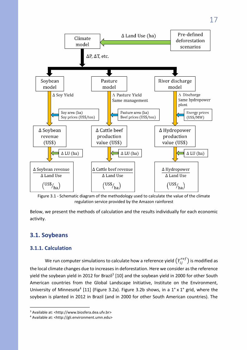
Each calculation makes use of specific models and depend on the availability of data (Figure
3.1). For soybeans, we use a soybean crop model, which uses weather information and
specific management information to calculate the soybean yield, in ton/ha. For the cattle
beef, we use a pasture growth model, which again uses weather information to calculate
pasture yield, in ton/ha. The pasture yield is converted to a production of weight of
beef/ha/year using a combination of regional and national data, depending on availability. For
calculation of the effect on hydropower energy, a river discharge model is used to convert
weather data in discharge data. Then, hydropower is calculated for the main hydropower
dams in Amazonia. All data of yearly production are converted to changes in revenue using
the average price of each commodity in the in a 12-month average (from June 2015 to May
2016): Soybean: US$ 338/ton; Beef: US$ 41/arroba1; electric energy: US$ 43/MWh2.
The change in revenue is calculated according to the availability of data. Impacts on soybean
production are calculated for the main producing regions in South America (Brazil, Argentina
and Paraguay). Impacts on cattle beef production are calculated for Brazil only, while impacts
on hydropower generation are calculated for the four main hydropower plants in operation
or under construction in Amazonia. The climate impacts caused by deforestation are more
important close to the deforested region, and decrease in magnitude with the distance to the
deforested region.
1 Arroba is a custom unit of weight for cattle in Brazil. 1 arroba = 32 lb (15 kg). 2 Sources: soybeans and cattle beef: www.cepea.org.br; electric energy: www.ccee.org.br.
17
Figure 3.1 - Schematic diagram of the methodology used to calculate the value of the climate
regulation service provided by the Amazon rainforest
Below, we present the methods of calculation and the results individually for each economic
activity.
3.1. Soybeans
3.1.1. Calculation
We run computer simulations to calculate how a reference yield (𝑌𝑖𝑗𝑟𝑒𝑓
) is modified as
the local climate changes due to increases in deforestation. Here we consider as the reference
yield the soybean yield in 2012 for Brazil3 [10] and the soybean yield in 2000 for other South
American countries from the Global Landscape Initiative, Institute on the Environment,
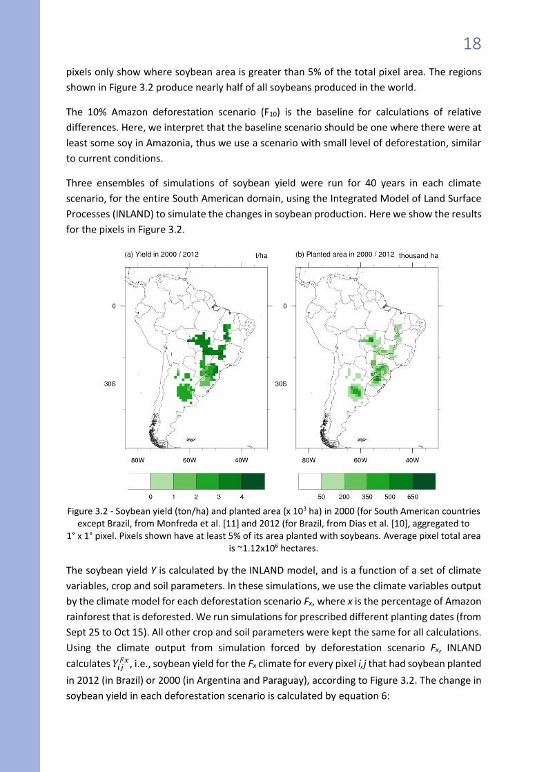
University of Minnesota4 [11] (Figure 3.2a). Figure 3.2b shows, in a 1° x 1° grid, where the
soybean is planted in 2012 in Brazil (and in 2000 for other South American countries). The
3 Available at: <http://www.biosfera.dea.ufv.br> 4 Available at: <http://gli.environment.umn.edu>
18
pixels only show where soybean area is greater than 5% of the total pixel area. The regions
shown in Figure 3.2 produce nearly half of all soybeans produced in the world.
The 10% Amazon deforestation scenario (F10) is the baseline for calculations of relative
differences. Here, we interpret that the baseline scenario should be one where there were at
least some soy in Amazonia, thus we use a scenario with small level of deforestation, similar
to current conditions.
Three ensembles of simulations of soybean yield were run for 40 years in each climate
scenario, for the entire South American domain, using the Integrated Model of Land Surface
Processes (INLAND) to simulate the changes in soybean production. Here we show the results
for the pixels in Figure 3.2.
Figure 3.2 - Soybean yield (ton/ha) and planted area (x 103 ha) in 2000 (for South American countries
except Brazil, from Monfreda et al. [11] and 2012 (for Brazil, from Dias et al. [10], aggregated to 1° x 1° pixel. Pixels shown have at least 5% of its area planted with soybeans. Average pixel total area
is ~1.12x10⁶ hectares.
The soybean yield Y is calculated by the INLAND model, and is a function of a set of climate
variables, crop and soil parameters. In these simulations, we use the climate variables output
by the climate model for each deforestation scenario Fx, where x is the percentage of Amazon
rainforest that is deforested. We run simulations for prescribed different planting dates (from
Sept 25 to Oct 15). All other crop and soil parameters were kept the same for all calculations.
Using the climate output from simulation forced by deforestation scenario Fx, INLAND
calculates 𝑌𝑖𝑗𝐹𝑥, i.e., soybean yield for the Fx climate for every pixel i,j that had soybean planted
in 2012 (in Brazil) or 2000 (in Argentina and Paraguay), according to Figure 3.2. The change in
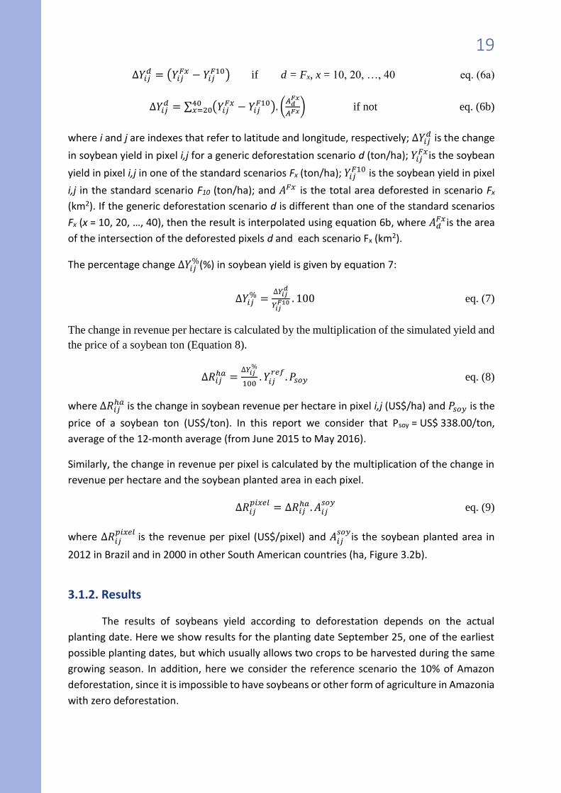
soybean yield in each deforestation scenario is calculated by equation 6:
19
∆𝑌𝑖𝑗𝑑 = (𝑌𝑖𝑗
𝐹𝑥 − 𝑌𝑖𝑗𝐹10) if d = Fx, x = 10, 20, …, 40 eq. (6a)
∆𝑌𝑖𝑗𝑑 = ∑ (𝑌𝑖𝑗
𝐹𝑥 − 𝑌𝑖𝑗𝐹10). (
𝐴𝑑𝐹𝑥
𝐴𝐹𝑥)40
𝑥=20 if not eq. (6b)
where i and j are indexes that refer to latitude and longitude, respectively; ∆𝑌𝑖𝑗𝑑 is the change
in soybean yield in pixel i,j for a generic deforestation scenario d (ton/ha); 𝑌𝑖𝑗𝐹𝑥 is the soybean
yield in pixel i,j in one of the standard scenarios Fx (ton/ha); 𝑌𝑖𝑗𝐹10 is the soybean yield in pixel
i,j in the standard scenario F10 (ton/ha); and 𝐴𝐹𝑥 is the total area deforested in scenario Fx
(km2). If the generic deforestation scenario d is different than one of the standard scenarios
Fx (x = 10, 20, …, 40), then the result is interpolated using equation 6b, where 𝐴𝑑𝐹𝑥 is the area
of the intersection of the deforested pixels d and each scenario Fx (km2).
The percentage change ∆𝑌𝑖𝑗%(%) in soybean yield is given by equation 7:
∆𝑌𝑖𝑗% =
∆𝑌𝑖𝑗𝑑
𝑌𝑖𝑗𝐹10 . 100 eq. (7)
The change in revenue per hectare is calculated by the multiplication of the simulated yield and
the price of a soybean ton (Equation 8).
∆𝑅𝑖𝑗ℎ𝑎 =
∆𝑌𝑖𝑗%
100. 𝑌𝑖𝑗
𝑟𝑒𝑓. 𝑃𝑠𝑜𝑦 eq. (8)
where ∆𝑅𝑖𝑗ℎ𝑎 is the change in soybean revenue per hectare in pixel i,j (US$/ha) and 𝑃𝑠𝑜𝑦 is the
price of a soybean ton (US$/ton). In this report we consider that Psoy = US$ 338.00/ton,
average of the 12-month average (from June 2015 to May 2016).
Similarly, the change in revenue per pixel is calculated by the multiplication of the change in
revenue per hectare and the soybean planted area in each pixel.
∆𝑅𝑖𝑗𝑝𝑖𝑥𝑒𝑙 = ∆𝑅𝑖𝑗
ℎ𝑎. 𝐴𝑖𝑗𝑠𝑜𝑦
eq. (9)
where ∆𝑅𝑖𝑗𝑝𝑖𝑥𝑒𝑙 is the revenue per pixel (US$/pixel) and 𝐴𝑖𝑗
𝑠𝑜𝑦is the soybean planted area in
2012 in Brazil and in 2000 in other South American countries (ha, Figure 3.2b).
3.1.2. Results
The results of soybeans yield according to deforestation depends on the actual
planting date. Here we show results for the planting date September 25, one of the earliest
possible planting dates, but which usually allows two crops to be harvested during the same
growing season. In addition, here we consider the reference scenario the 10% of Amazon
deforestation, since it is impossible to have soybeans or other form of agriculture in Amazonia
with zero deforestation.
20
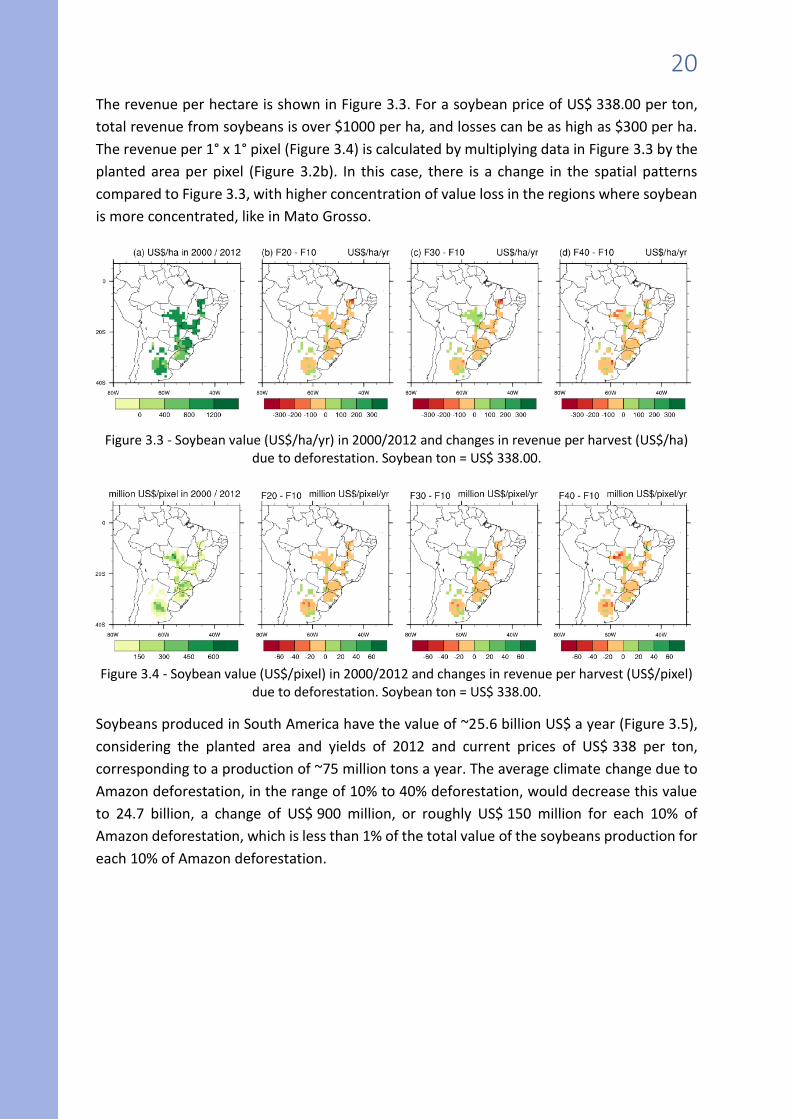
The revenue per hectare is shown in Figure 3.3. For a soybean price of US$ 338.00 per ton,
total revenue from soybeans is over $1000 per ha, and losses can be as high as $300 per ha.
The revenue per 1° x 1° pixel (Figure 3.4) is calculated by multiplying data in Figure 3.3 by the
planted area per pixel (Figure 3.2b). In this case, there is a change in the spatial patterns
compared to Figure 3.3, with higher concentration of value loss in the regions where soybean
is more concentrated, like in Mato Grosso.
Figure 3.3 - Soybean value (US$/ha/yr) in 2000/2012 and changes in revenue per harvest (US$/ha)
due to deforestation. Soybean ton = US$ 338.00.
Figure 3.4 - Soybean value (US$/pixel) in 2000/2012 and changes in revenue per harvest (US$/pixel)
due to deforestation. Soybean ton = US$ 338.00.
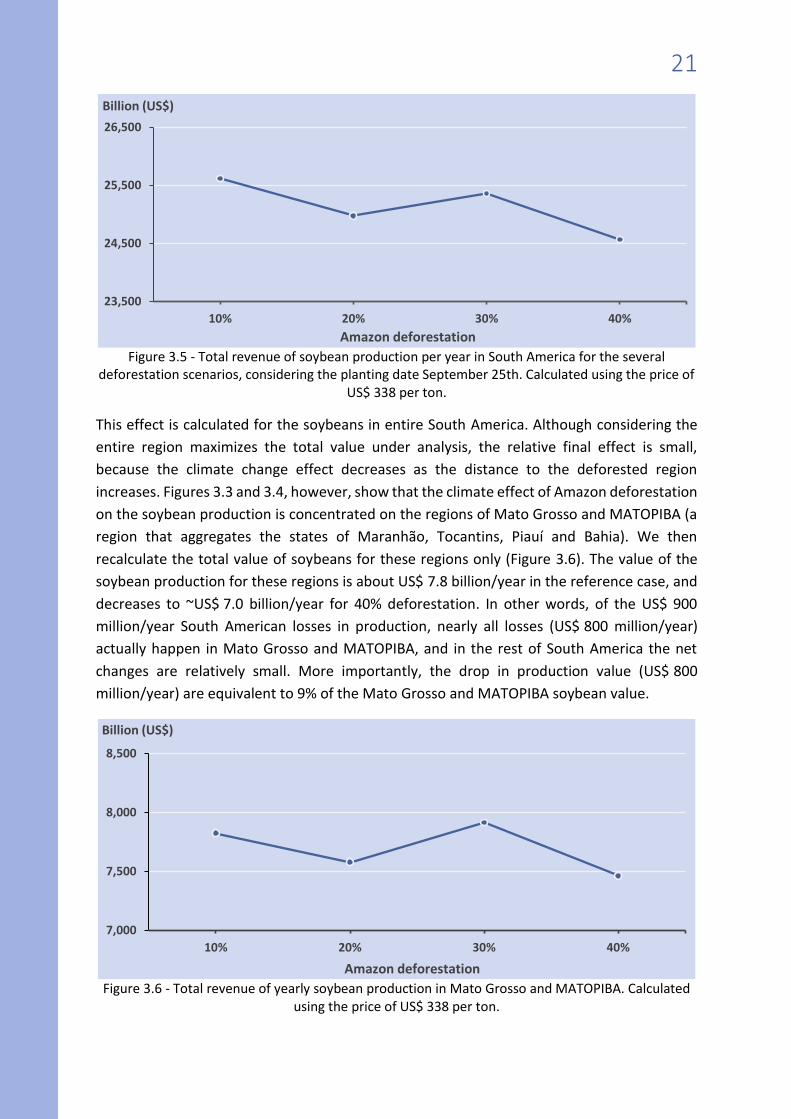
Soybeans produced in South America have the value of ~25.6 billion US$ a year (Figure 3.5),
considering the planted area and yields of 2012 and current prices of US$ 338 per ton,
corresponding to a production of ~75 million tons a year. The average climate change due to
Amazon deforestation, in the range of 10% to 40% deforestation, would decrease this value
to 24.7 billion, a change of US$ 900 million, or roughly US$ 150 million for each 10% of
Amazon deforestation, which is less than 1% of the total value of the soybeans production for
each 10% of Amazon deforestation.
21
Figure 3.5 - Total revenue of soybean production per year in South America for the several deforestation scenarios, considering the planting date September 25th. Calculated using the price of
US$ 338 per ton.
This effect is calculated for the soybeans in entire South America. Although considering the
entire region maximizes the total value under analysis, the relative final effect is small,
because the climate change effect decreases as the distance to the deforested region
increases. Figures 3.3 and 3.4, however, show that the climate effect of Amazon deforestation
on the soybean production is concentrated on the regions of Mato Grosso and MATOPIBA (a
region that aggregates the states of Maranhão, Tocantins, Piauí and Bahia). We then
recalculate the total value of soybeans for these regions only (Figure 3.6). The value of the
soybean production for these regions is about US$ 7.8 billion/year in the reference case, and
decreases to ~US$ 7.0 billion/year for 40% deforestation. In other words, of the US$ 900
million/year South American losses in production, nearly all losses (US$ 800 million/year)
actually happen in Mato Grosso and MATOPIBA, and in the rest of South America the net
changes are relatively small. More importantly, the drop in production value (US$ 800
million/year) are equivalent to 9% of the Mato Grosso and MATOPIBA soybean value.
Figure 3.6 - Total revenue of yearly soybean production in Mato Grosso and MATOPIBA. Calculated using the price of US$ 338 per ton.
23,500
24,500
25,500
26,500
10% 20% 30% 40%
Billion (US$)
Amazon deforestation
7,000
7,500
8,000
8,500
10% 20% 30% 40%
Billion (US$)
Amazon deforestation
22
3.2. Cattle beef
3.2.1. Calculation
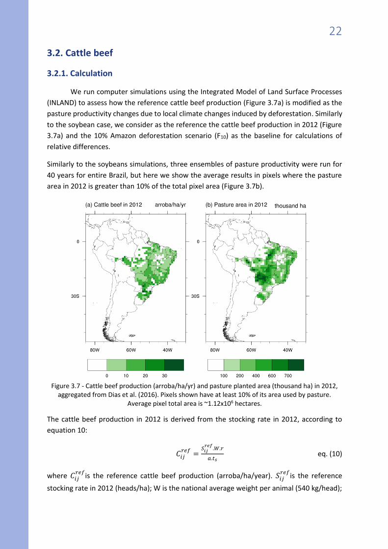
We run computer simulations using the Integrated Model of Land Surface Processes
(INLAND) to assess how the reference cattle beef production (Figure 3.7a) is modified as the
pasture productivity changes due to local climate changes induced by deforestation. Similarly
to the soybean case, we consider as the reference the cattle beef production in 2012 (Figure
3.7a) and the 10% Amazon deforestation scenario (F10) as the baseline for calculations of
relative differences.
Similarly to the soybeans simulations, three ensembles of pasture productivity were run for
40 years for entire Brazil, but here we show the average results in pixels where the pasture
area in 2012 is greater than 10% of the total pixel area (Figure 3.7b).
Figure 3.7 - Cattle beef production (arroba/ha/yr) and pasture planted area (thousand ha) in 2012,
aggregated from Dias et al. (2016). Pixels shown have at least 10% of its area used by pasture. Average pixel total area is ~1.12x10⁶ hectares.
The cattle beef production in 2012 is derived from the stocking rate in 2012, according to
equation 10:
𝐶𝑖𝑗𝑟𝑒𝑓
=𝑆𝑖𝑗
𝑟𝑒𝑓.𝑊.𝑟
𝑎.𝑡𝑠 eq. (10)
where 𝐶𝑖𝑗𝑟𝑒𝑓
is the reference cattle beef production (arroba/ha/year). 𝑆𝑖𝑗𝑟𝑒𝑓
is the reference
stocking rate in 2012 (heads/ha); W is the national average weight per animal (540 kg/head);
23
r is the average ratio dead weight/live weight (r = 0.41); a is the conversion factor from arroba
to kg (a = 15kg/arroba); and ts is the average animal age at slaughter (ts = 2 years).
The change in pasture productivity P in each deforestation scenario is calculated by equation
11:
∆𝑃𝑖𝑗𝑑 = (𝑃𝑖𝑗
𝐹𝑥 − 𝑃𝑖𝑗𝐹10) if d = Fx, x = 10, 20, …, 40 eq. (11a)
∆𝑃𝑖𝑗𝑑 = ∑ (𝑃𝑖𝑗
𝐹𝑥 − 𝑃𝑖𝑗𝐹10). (
𝐴𝑑𝐹𝑥
𝐴𝐹𝑥)40𝑥=20 if not eq. (11b)
where i and j are indexes that refer to latitude and longitude, respectively; ∆𝑃𝑖𝑗𝑑 is the change
in pasture productivity in pixel i,j (kg-C.m-2.yr-1); 𝑃𝑖𝑗𝐹𝑥 is the pasture productivity in pixel i,j
scenario Fx (kg-C.m-2.yr-1); 𝑃𝑖𝑗𝐹10 is the pasture productivity in pixel i,j in scenario F10 (kg-C.m-
2.yr-1) and 𝐴𝐹𝑥 is the total area of scenario Fx (km2). Similarly to the soybean case, if the generic
deforestation scenario d is different than one of the standard scenarios Fx (x = 10, 20, …, 40),
then the result is interpolated using equation 11b.
The percentage change ∆𝑃𝑖𝑗% (%) in pasture productivity is given by equation 12:
∆𝑃𝑖𝑗% =
∆𝑃𝑖𝑗𝑑
𝑃𝑖𝑗𝐹10 . 100 eq. (12)
Equation 13 then calculates the change in cattle beef production:
𝐶𝑖𝑗𝑑 =
𝐶𝑖𝑗𝑟𝑒𝑓
.∆𝑃𝑖𝑗%
100 eq. (13)
The revenue per hectare is calculated by the multiplication of the cattle beef production per
hectare per year and the price of the arroba (Equation 14).
𝐸𝑖𝑗ℎ𝑎 = 𝐶𝑖𝑗
𝑑 . 𝑃𝑎𝑟𝑟𝑜𝑏𝑎 eq. (14)
where 𝐸𝑖𝑗ℎ𝑎 is the cattle beef revenue per hectare per year in pixel i,j (US$/ha/yr) and 𝑃𝑎𝑟𝑟𝑜𝑏𝑎
is the price of an arroba of dead weight (US$/arroba). In this report we consider
Parroba = US$ 41, the 12-month average (from June 2015 to May 2016).
Similarly, the revenue per pixel is calculated by the multiplication of the revenue per hectare
and the pasture area (in hectares) (Equation 15).
𝐸𝑖𝑗𝑝𝑖𝑥𝑒𝑙 = 𝐸𝑖𝑗
ℎ𝑎 . 𝐴𝑖𝑗𝑝𝑎𝑠𝑡𝑢𝑟𝑒
eq. (15)
where 𝐸𝑖𝑗𝑝𝑖𝑥𝑒𝑙 is the revenue per pixel (US$/pixel) and 𝐴𝑖𝑗
𝑝𝑎𝑠𝑡𝑢𝑟𝑒is the pasture area per pixel i,j
in 2012 (ha, Figure 3.7b).
24
3.2.2. Results
The changes in production assumes that the changes in pasture yield (due to climate
change) are translated directly to the production of beef, without any measures of adaptation
by the cattle rancher, like reductions in the stocking rate (head/ha) or increases in animal age
at slaughter to accommodate the lower pasture yield. Production of cattle beef per unit area
per year is calculated by equation 10 using data from Figure 3.7a. Changes in production are
calculated using equation 12.
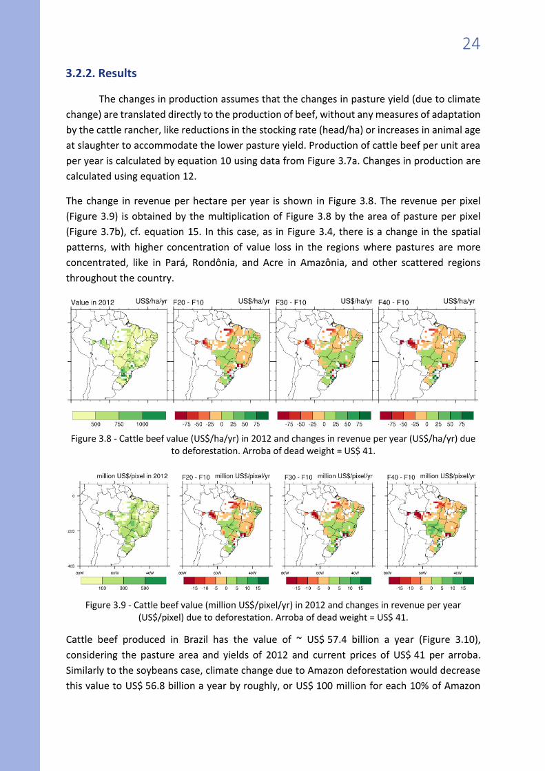
The change in revenue per hectare per year is shown in Figure 3.8. The revenue per pixel
(Figure 3.9) is obtained by the multiplication of Figure 3.8 by the area of pasture per pixel
(Figure 3.7b), cf. equation 15. In this case, as in Figure 3.4, there is a change in the spatial
patterns, with higher concentration of value loss in the regions where pastures are more
concentrated, like in Pará, Rondônia, and Acre in Amazônia, and other scattered regions
throughout the country.
Figure 3.8 - Cattle beef value (US$/ha/yr) in 2012 and changes in revenue per year (US$/ha/yr) due
to deforestation. Arroba of dead weight = US$ 41.
Figure 3.9 - Cattle beef value (million US$/pixel/yr) in 2012 and changes in revenue per year
(US$/pixel) due to deforestation. Arroba of dead weight = US$ 41.
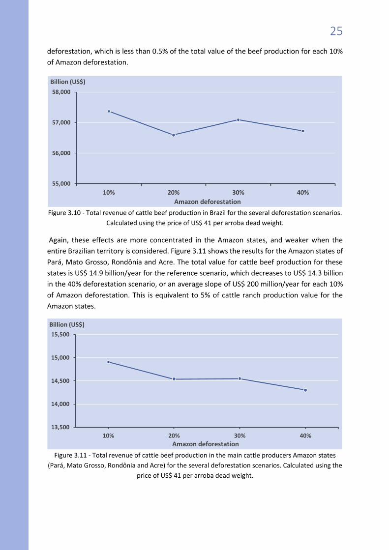
Cattle beef produced in Brazil has the value of ~ US$ 57.4 billion a year (Figure 3.10),
considering the pasture area and yields of 2012 and current prices of US$ 41 per arroba.
Similarly to the soybeans case, climate change due to Amazon deforestation would decrease
this value to US$ 56.8 billion a year by roughly, or US$ 100 million for each 10% of Amazon
25
deforestation, which is less than 0.5% of the total value of the beef production for each 10%
of Amazon deforestation.
Figure 3.10 - Total revenue of cattle beef production in Brazil for the several deforestation scenarios.
Calculated using the price of US$ 41 per arroba dead weight.
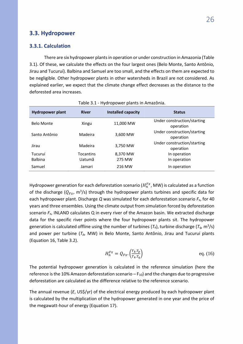
Again, these effects are more concentrated in the Amazon states, and weaker when the
entire Brazilian territory is considered. Figure 3.11 shows the results for the Amazon states of
Pará, Mato Grosso, Rondônia and Acre. The total value for cattle beef production for these
states is US$ 14.9 billion/year for the reference scenario, which decreases to US$ 14.3 billion
in the 40% deforestation scenario, or an average slope of US$ 200 million/year for each 10%
of Amazon deforestation. This is equivalent to 5% of cattle ranch production value for the
Amazon states.
Figure 3.11 - Total revenue of cattle beef production in the main cattle producers Amazon states
(Pará, Mato Grosso, Rondônia and Acre) for the several deforestation scenarios. Calculated using the
price of US$ 41 per arroba dead weight.
55,000
56,000
57,000
58,000
10% 20% 30% 40%
Billion (US$)
Amazon deforestation
13,500
14,000
14,500
15,000
15,500
10% 20% 30% 40%
Billion (US$)
Amazon deforestation
26
3.3. Hydropower
3.3.1. Calculation
There are six hydropower plants in operation or under construction in Amazonia (Table
3.1). Of these, we calculate the effects on the four largest ones (Belo Monte, Santo Antônio,
Jirau and Tucuruí). Balbina and Samuel are too small, and the effects on them are expected to
be negligible. Other hydropower plants in other watersheds in Brazil are not considered. As
explained earlier, we expect that the climate change effect decreases as the distance to the
deforested area increases.
Table 3.1 - Hydropower plants in Amazônia.
Hydropower plant River Installed capacity Status
Belo Monte Xingu 11,000 MW Under construction/starting
operation
Santo Antônio Madeira 3,600 MW Under construction/starting
operation
Jirau Madeira 3,750 MW Under construction/starting
operation Tucuruí Tocantins 8,370 MW In operation Balbina Uatumã 275 MW In operation
Samuel Jamari 216 MW In operation
Hydropower generation for each deforestation scenario (𝐻𝑛𝐹𝑥, MW) is calculated as a function
of the discharge (𝑄𝐹𝑥, m3/s) through the hydropower plants turbines and specific data for
each hydropower plant. Discharge Q was simulated for each deforestation scenario Fx, for 40
years and three ensembles. Using the climate output from simulation forced by deforestation
scenario Fx, INLAND calculates Q in every river of the Amazon basin. We extracted discharge
data for the specific river points where the four hydropower plants sit. The hydropower
generation is calculated offline using the number of turbines (Tk), turbine discharge (Tq, m3/s)
and power per turbine (Tp, MW) in Belo Monte, Santo Antônio, Jirau and Tucuruí plants
(Equation 16, Table 3.2).
𝐻𝑛𝐹𝑥 = 𝑄𝐹𝑥. (
𝑇𝑘.𝑇𝑝
𝑇𝑘.𝑇𝑞) eq. (16)
The potential hydropower generation is calculated in the reference simulation (here the
reference is the 10% Amazon deforestation scenario – F10) and the changes due to progressive
deforestation are calculated as the difference relative to the reference scenario.
The annual revenue (E, US$/yr) of the electrical energy produced by each hydropower plant
is calculated by the multiplication of the hydropower generated in one year and the price of
the megawatt-hour of energy (Equation 17).
27
𝐸 = 𝐻𝑛𝐹𝑥. 𝑛 . 𝑃𝑀𝑊ℎ eq. (17)
where n is the number of hours in one year (n = 8760) and 𝑃𝑀𝑊ℎis the price of a megawatt-
hour of energy (US$). In this report we use 𝑃𝑀𝑊ℎ = US$ 43/MWh, which is the average price
of liquidation of differences in a 12-month average (from June 2015 to May 2016) for the
northern region in Brazil, calculated during the period of the day of maximum demand.
Table 3.2 - Technical information of Belo Monte, Santo Antônio, Jirau and Tucuruí hydropower plants.
Hydroelectric Plant
Number of turbines
Turbine discharge (m3/s)
Turbine power (MW)
Installed capacity (MW)
Belo Monte 18 775 611 11,000
Santo Antônio 50 565 71.36 3,568
Jirau 50 541 75 3,750
Tucuruí 12 576 350
8,325 11 679 375
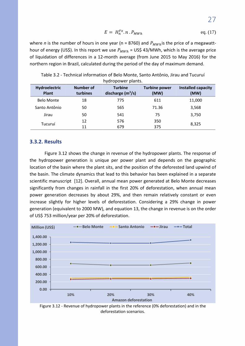
3.3.2. Results
Figure 3.12 shows the change in revenue of the hydropower plants. The response of
the hydropower generation is unique per power plant and depends on the geographic
location of the basin where the plant sits, and the position of the deforested land upwind of
the basin. The climate dynamics that lead to this behavior has been explained in a separate
scientific manuscript [12]. Overall, annual mean power generated at Belo Monte decreases
significantly from changes in rainfall in the first 20% of deforestation, when annual mean
power generation decreases by about 29%, and then remain relatively constant or even
increase slightly for higher levels of deforestation. Considering a 29% change in power
generation (equivalent to 2000 MW), and equation 13, the change in revenue is on the order
of US$ 753 million/year per 20% of deforestation.
Figure 3.12 - Revenue of hydropower plants in the reference (0% deforestation) and in the deforestation scenarios.
0.00
200.00
400.00
600.00
800.00
1,000.00
1,200.00
1,400.00
10% 20% 30% 40%
Million (US$)
Amazon deforestation
Belo Monte Santo Antonio Jirau Total
28
3.4. Statistical significance of the results
The revenue variables calculated in this project are, in general, not normally
distributed, which does not recommend the use of standard parametric statistics such as the
t-test. Instead, we used non-parametric statistics, which are more powerful when the
probability distribution of the data is unkown. The analysis presented here is based on the
work by Anderson [13].
Consider a random variable x with an unknown but continuous cumulative distribution F(x),
such that F(a) = 0 and F(b) = 1 for known finite numbers a and b (a < b). Let x(1) < x(2) < … < x(n)
be the ordered observations in the sample of size n from F(x), such that x(0) = a and x(n+1) = b.
The empirical cumulative distribution in [a,b] is
F(x) = j/n, x(j) ≤ x ≤ x(j+1), j = 0, 1, ... , n. eq. (18)
Let and be numbers such that the probability of
F(x) – ≤ F(x) ≤ F(x) + eq. (19)
is 1 – , i.e., the confidence interval of x. The confidence limits for the mean are given by the
interval
r
j
j
n
snj
j xrbn
xsaxn
x11
1,
1. For a bilateral test with = 0.05 and a
time series of n = 40, s = 1, so that = s/n = 0.025, and r = 39, so that = r/n = 0.975.
In this work, we calculated the statistical significance of the difference between two means,
the mean of the treatment T ( Tx ) and the mean of the control C ( Cx ). For a discrete time
series like the ones under study, the probability of Tx < Cx is smaller than the probability s/n,
where s is order of the first number of the control series so that Ts
C xx )( :
n
sxP CT x eq. (20)
Similarly, the probability of Tx > Cx is smaller than the probability 1-r/n, where r is the order
of the first number of the control series so that Tr
C xx )( :
n
rxP CT 1x eq. (21)
The online platform plots the differences of the means and their statistical significance is
available by clicking on any grid cell where the difference has been calculated. Typically, the
significance of the differences is higher for pixels close to Amazonia, where deforestation
happens. For these pixels, significance is higher for rainfall (P <0.1), intermediate for
hydropower generations (P~0.1-0.2) and smaller for agriculture (P~0.3-0.5). Please check the
online platform (described in Section 5) for the actual results.
29
4. Estimation of the climate regulation service provided
by the Amazon
4.1. Calculation
In brief, the changes in revenue (ΔR) in agricultural production and hydropower
generation are atributed to each pixel of the Amazon rainforest following the proportional
division of the changes in revenue for each economic activity by the number of pixels with
additional deforestation in each land use change scenario (s). We also calculated the changes
in revenue to each hectare (ha) of the foret area basically dividing these results by the pixel
area. These calculations are detailed as follows.
For soybeans and cattle beef, the revenue associated to the climate of each deforestation
scenario s ( s
agR , in US$) is calculated by summing the production output per pixel with
agricultural activity pxa ( s
pxaO , in tons per pixel) in all soy/cattle pixels in each scenario s. The
sum (in tons) is then converted to dollars using the market price (P, US$/ton) of each good,
according to equation 22.
Npxa
pxa
s
pxa
s
ag OPR1
eq. (22)
Where Npxv is the number of pixels whith soy/beef production in South America.
The change in agriculture revenue due to deforestation ( agR , US$) is then calculated
between two consecutive scenarios (s and s-1, Equation 23).
1
s
ag
s
agag RRR eq. (23)
The climate regulation ecosystem service provided to agriculture ( agV , US$) by each ha
located in each forest pixel (pxf) is then calculated by dividing the change in revenue by the
number of pixels with additional deforestation in each land use change scenario (Npxf) and the
forest pixel area (Apxf, in ha), as in equation 24.
pxfpxf
agag
agAN
R
LU
RV
eq. (24)
Similarly, for hydropower, the revenue associated to the climate of each deforestation
scenario ( s
hyR , in US$) is calculated by summing the power generated (W, in MW) by each
hydropower plant (h) in the scenario s and converted to dollars using the market price (PE,
US$/MW) according to equation 25.
30
Nh
h
s
hE
s
hy WPR1
eq. (25)
Where Nh is the number of hydropower plants considered in this study.
The change in revenue due to deforestation ( hyR , US$) is then calculated between two
consecutive scenarios (s and s-1, Equation 26).
1
s
hy
s
hyhy RRR eq. (26)
The climate regulation ecosystem service provided to hydropower generation ( hyV , US$) by
each ha located in each forest pixel (pxf) is then calculated by dividing the change in revenue
by the number of pixels with additional deforestation in each land use change scenario (Npxf)
and the forest pixel area (Apxf, in ha), as in equation 27.
pxfpxf
hyhy
hyAN
R
LU
RV
eq. (27)
Finally, the total climate regulation ecosystem service provided by the Amazon rainforest
totalV , US$) is then calculated by adding the values calculated in equations 24 and 28:
hyagtotal VVV eq. (28)
4.2. Results
Initially, it is important to highlight that atmospheric circulation and climate patterns
respond in a non-linear way to deforestation. Although the general trend is a decrease in
precipitation with the increase of deforestation, the rate of change is not constant [1]. In
addition, intermediate levels of deforestation can lead to enhanced convection and as a
result, local rainfall may increase [14].
The economic activities also respond non-linearly, according to the precipitation patterns and
to their geographic location and the characteristics of each activity. Soybeans production
depends on rainfall and other climate variables during the growing season only (four months).
Cattle beef production depends on yearly rainfall, but it is more sensitive in particular to dry
season rainfall. Hydropower generation, on the other hand, does not respond to changes in
rainfall during the rainiest months of the rainy season, when the plant is already working at
maximum capacity.
The revenue of the climate regulation ecosystem service provided by the Amazon rainforest
varies spatially in signal and magnitude over the forest area (Figure 4.1) and the service
31
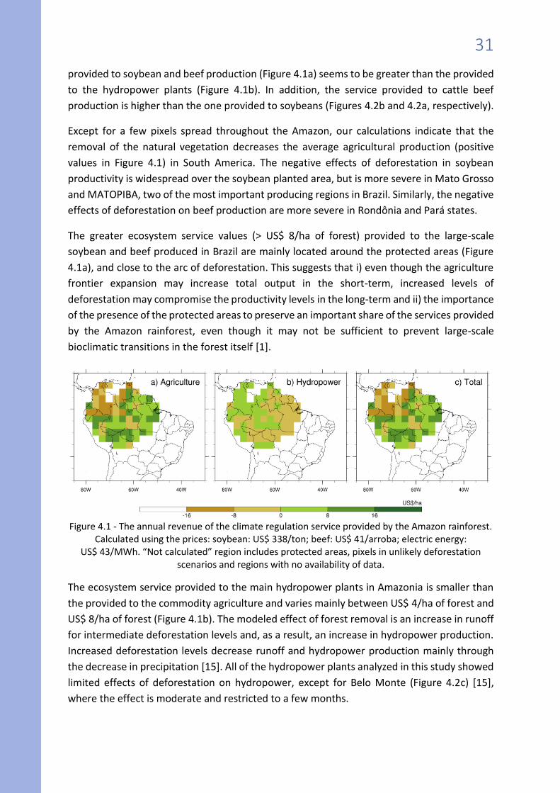
provided to soybean and beef production (Figure 4.1a) seems to be greater than the provided
to the hydropower plants (Figure 4.1b). In addition, the service provided to cattle beef
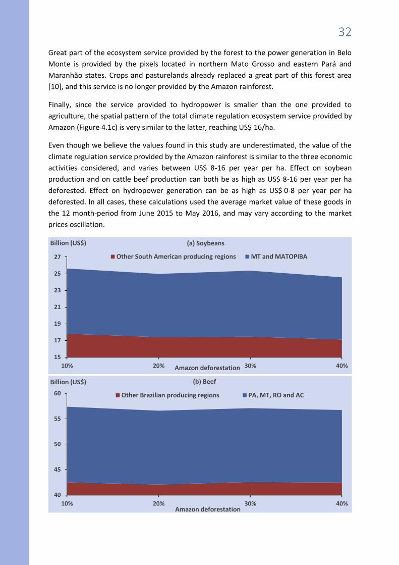
production is higher than the one provided to soybeans (Figures 4.2b and 4.2a, respectively).
Except for a few pixels spread throughout the Amazon, our calculations indicate that the
removal of the natural vegetation decreases the average agricultural production (positive
values in Figure 4.1) in South America. The negative effects of deforestation in soybean
productivity is widespread over the soybean planted area, but is more severe in Mato Grosso
and MATOPIBA, two of the most important producing regions in Brazil. Similarly, the negative
effects of deforestation on beef production are more severe in Rondônia and Pará states.
The greater ecosystem service values (> US$ 8/ha of forest) provided to the large-scale
soybean and beef produced in Brazil are mainly located around the protected areas (Figure
4.1a), and close to the arc of deforestation. This suggests that i) even though the agriculture
frontier expansion may increase total output in the short-term, increased levels of
deforestation may compromise the productivity levels in the long-term and ii) the importance
of the presence of the protected areas to preserve an important share of the services provided
by the Amazon rainforest, even though it may not be sufficient to prevent large-scale
bioclimatic transitions in the forest itself [1].
Figure 4.1 - The annual revenue of the climate regulation service provided by the Amazon rainforest.
Calculated using the prices: soybean: US$ 338/ton; beef: US$ 41/arroba; electric energy: US$ 43/MWh. “Not calculated” region includes protected areas, pixels in unlikely deforestation
scenarios and regions with no availability of data.
The ecosystem service provided to the main hydropower plants in Amazonia is smaller than
the provided to the commodity agriculture and varies mainly between US$ 4/ha of forest and
US$ 8/ha of forest (Figure 4.1b). The modeled effect of forest removal is an increase in runoff
for intermediate deforestation levels and, as a result, an increase in hydropower production.
Increased deforestation levels decrease runoff and hydropower production mainly through
the decrease in precipitation [15]. All of the hydropower plants analyzed in this study showed
limited effects of deforestation on hydropower, except for Belo Monte (Figure 4.2c) [15],
where the effect is moderate and restricted to a few months.
32
Great part of the ecosystem service provided by the forest to the power generation in Belo
Monte is provided by the pixels located in northern Mato Grosso and eastern Pará and
Maranhão states. Crops and pasturelands already replaced a great part of this forest area
[10], and this service is no longer provided by the Amazon rainforest.
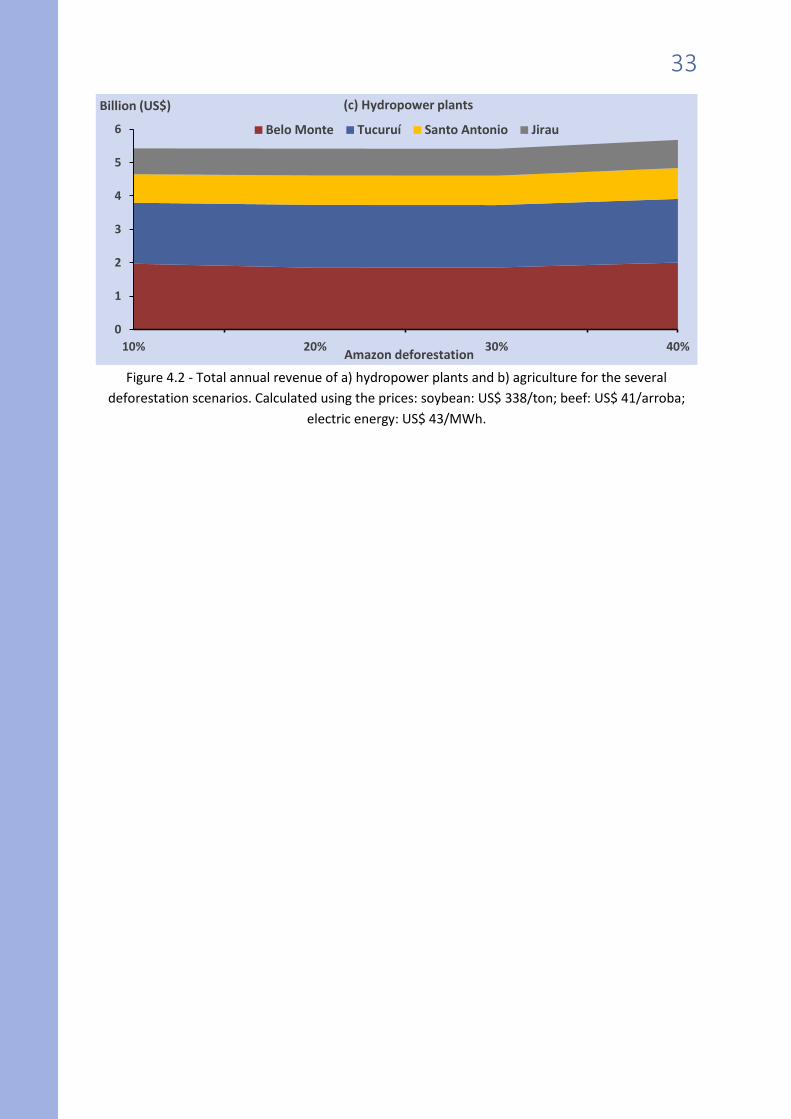
Finally, since the service provided to hydropower is smaller than the one provided to
agriculture, the spatial pattern of the total climate regulation ecosystem service provided by
Amazon (Figure 4.1c) is very similar to the latter, reaching US$ 16/ha.
Even though we believe the values found in this study are underestimated, the value of the
climate regulation service provided by the Amazon rainforest is similar to the three economic
activities considered, and varies between US$ 8-16 per year per ha. Effect on soybean
production and on cattle beef production can both be as high as US$ 8-16 per year per ha
deforested. Effect on hydropower generation can be as high as US$ 0-8 per year per ha
deforested. In all cases, these calculations used the average market value of these goods in
the 12 month-period from June 2015 to May 2016, and may vary according to the market
prices oscillation.
15
17
19
21
23
25
27
10% 20% 30% 40%
Billion (US$) (a) Soybeans
Other South American producing regions MT and MATOPIBA
Amazon deforestation
40
45
50
55
60
10% 20% 30% 40%
Billion (US$) (b) Beef
Other Brazilian producing regions PA, MT, RO and AC
Amazon deforestation
33
Figure 4.2 - Total annual revenue of a) hydropower plants and b) agriculture for the several
deforestation scenarios. Calculated using the prices: soybean: US$ 338/ton; beef: US$ 41/arroba;
electric energy: US$ 43/MWh.
0
1
2
3
4
5
6
10% 20% 30% 40%
Billion (US$)
Amazon deforestation
(c) Hydropower plants
Belo Monte Tucuruí Santo Antonio Jirau
34
5. Online Platforms
Two online platforms were developed for this project. The Deforestation and Rainfall
Platform was developed by the FUNARBE/UFV team and describes in detail the effects of the
deforestation on climate and on the economic activities. The main results of this platform is
then mirrored at the main Online Platform for this project, the Amazon Ecoservices Platform,
developed by the FUNDEP/UFMG team.
An online platform – Deforestation and Rainfall – (available at
http://www.biosfera.dea.ufv.br/en-US/deforestation-and-rainfall) was developed to include
the effects of Amazon deforestation on rainfall, soybean and cattle beef production and
hydropower according to the methodologies described above. In summary, we use the web
tools GDAL (Geospatial Data Abstraction Library) to process and the OpenLayers library to
visualize the data, and MapServer to draw the maps.
Deforestation and Rainfall has a responsive and intuitive interface that has been tested in
many browsers as Mozilla Firefox, Google Chrome, Opera, Apple Safari, Microsoft Internet
Explorer and Microsoft Edge. The platform works on PCs, Macs and tablets, as long as the
screen resolution is at least 1024 x 768 pixels (includes all iPads models). For better results we
recommend standard Full HD monitors (1920 x 1080 pixels).
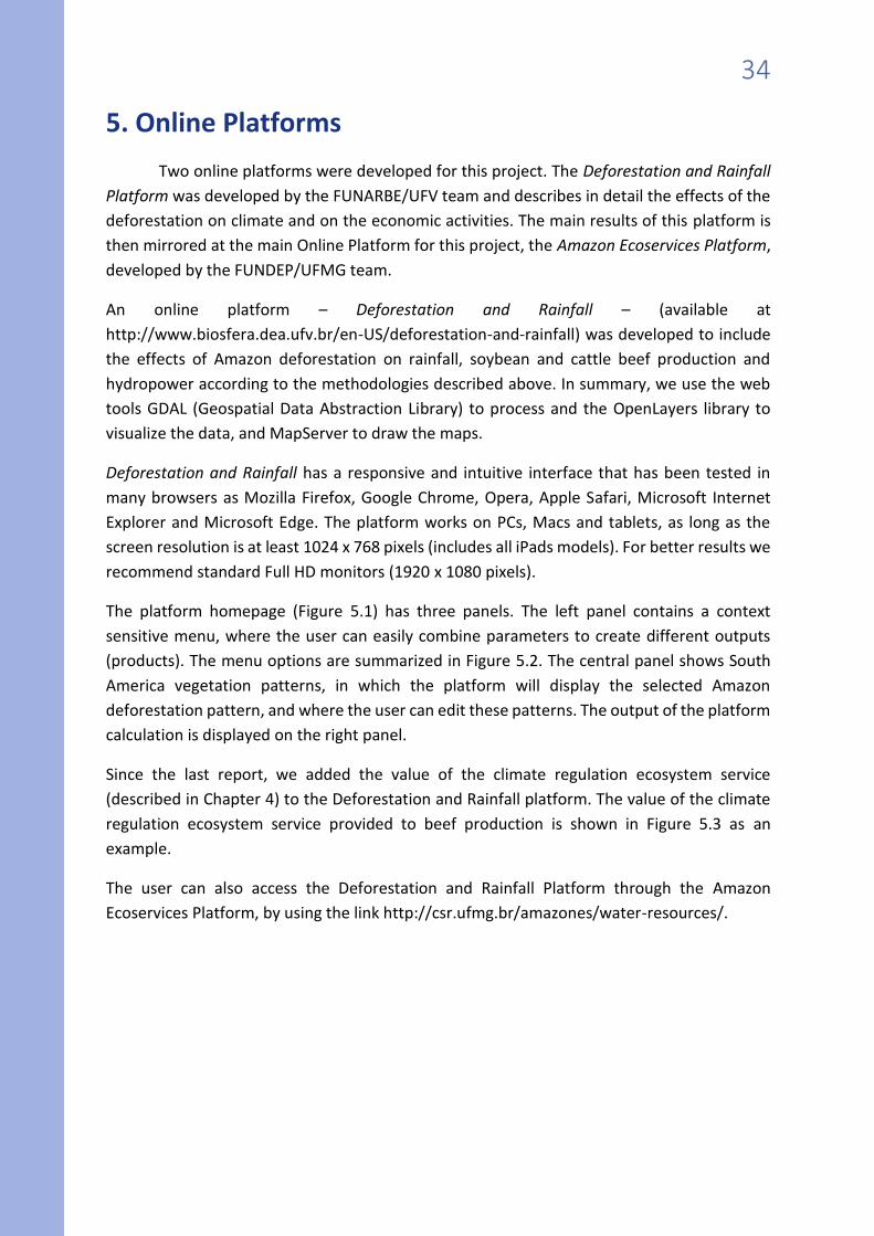
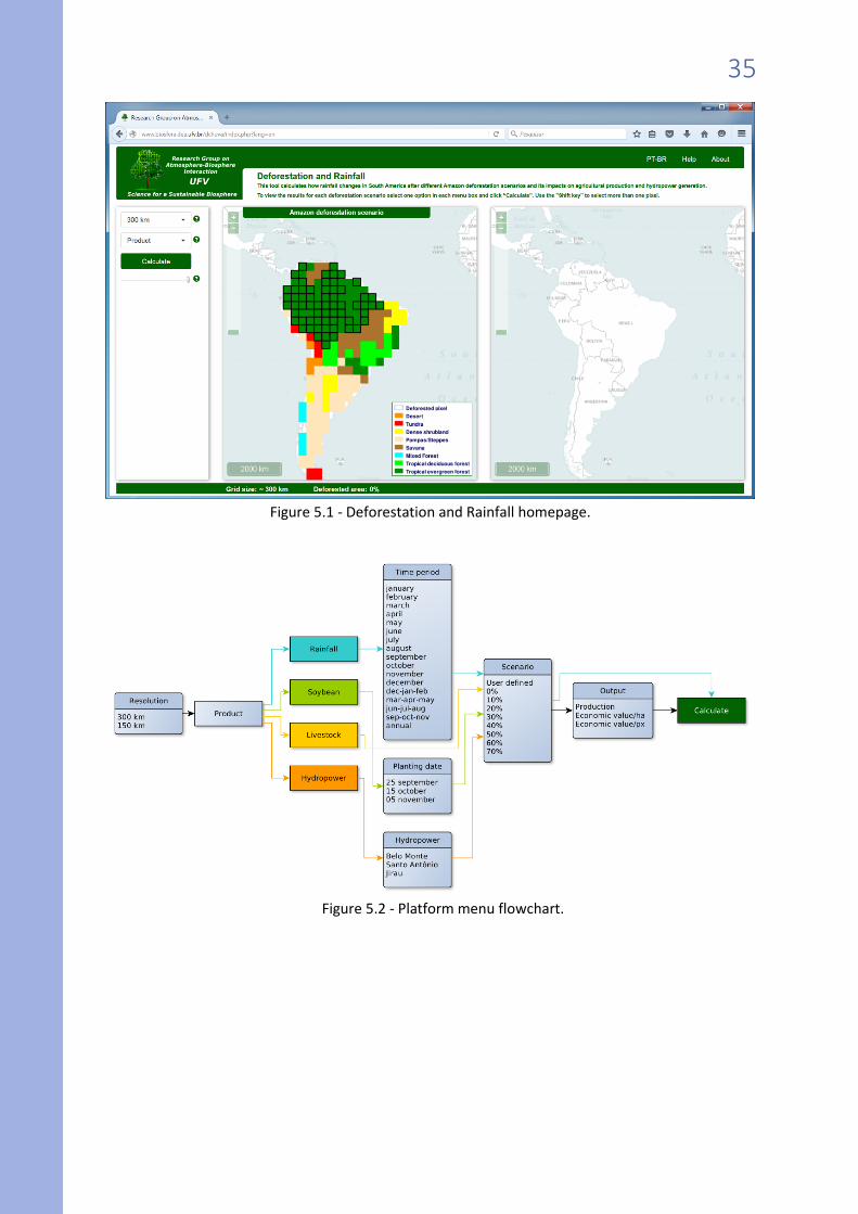
The platform homepage (Figure 5.1) has three panels. The left panel contains a context
sensitive menu, where the user can easily combine parameters to create different outputs
(products). The menu options are summarized in Figure 5.2. The central panel shows South
America vegetation patterns, in which the platform will display the selected Amazon
deforestation pattern, and where the user can edit these patterns. The output of the platform
calculation is displayed on the right panel.
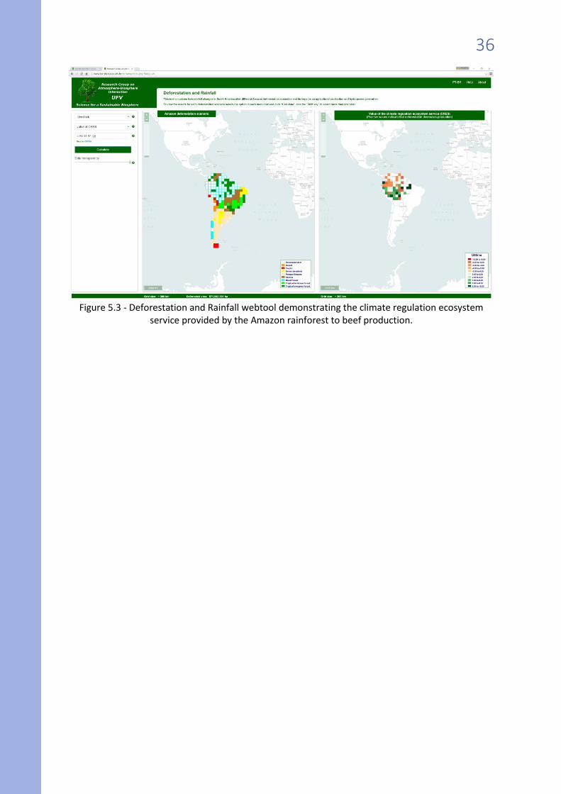
Since the last report, we added the value of the climate regulation ecosystem service
(described in Chapter 4) to the Deforestation and Rainfall platform. The value of the climate
regulation ecosystem service provided to beef production is shown in Figure 5.3 as an
example.
The user can also access the Deforestation and Rainfall Platform through the Amazon
Ecoservices Platform, by using the link http://csr.ufmg.br/amazones/water-resources/.
35
Figure 5.1 - Deforestation and Rainfall homepage.
Figure 5.2 - Platform menu flowchart.
36
Figure 5.3 - Deforestation and Rainfall webtool demonstrating the climate regulation ecosystem
service provided by the Amazon rainforest to beef production.
37
6. Final Remarks
The revenue estimates are subject to a few caveats. First, these can be considered
conservative estimates. The rainforest provides other services related to the hydrological
cycle, including maintain navigation year around and helping control floods. Considering these
additional services would increase the value of the hydrological cycle regulation service
provided by each unit of rainforest area.
Second, these values are not constant. They tend to be higher per ha for lower levels of
deforestation, decreasing per ha when deforestation increases. On the other hand, even if the
value per unit of area decreases, the total value tends to increase with the level of
deforestation, as it is the result of the value per unit of area multiplied by the total area
deforested.
Third, this a permanent service provided by the rainforest. Reducing this service by
deforestation has permanent effects. In a sense, this increases its relative value when
compared to other stock-type ecosystem services, such as preservation of biodiversity, that
are provided only once, and not every year.
Finally, the effects studied are stronger in Amazonia. The relative effect on the local economic
activities is a loss of 10-30%, depending on the economic activity considered. Policy makers
and other Amazon agriculture and energy businesses must be aware of these numbers, and
consider them while planning their activities. This is true particularly for the agribusiness
sector, at the same time the main sector responsible for deforestation and one of the main
sectors affected by the climate change introduced by deforestation.
38
7. References
1. Pires, G.F. and M.H. Costa, Deforestation causes different subregional effects on the Amazon bioclimatic equilibrium. Geophys. Res. Lett, 2013. 40(14): p. 3618-3623.
2. Vera, C.S., et al., Toward a Unified View of the American Monsoon Systems. Journal of Climate, 2006. 19: p. 4977-5000.
3. Marengo, J.A., et al., Recent developments on the South American monsoon system. Int. J. Climatol, 2012. 32(1): p. 1-21.
4. Dirmeyer, P.A. and K.L. Brubaker, Characterization of the Global Hydrologic Cycle from a Back-Trajectory Analysis of Atmospheric Water Vapor. Journal of Hydrometeorology, 2007. 8: p. 20-37.
5. Henderson-Sellers, A., K. McGuffie, and H. Zhang, Stable isotopes as validation tools for global climate model predictions of the impact of Amazonian deforestation. Journal of Climate, 2002. 15(18): p. 2664-2677.
6. Stohl, A. and P.A. James, Lagrangian Analysis of the Atmospheric Branch of the Global Water Cycle. Part I: Method Description, Validation, and Demonstration for the August 2002 Flooding in Central Europe. Journal of Hydrometeorology, 2004. 5(4): p. 656-678.
7. Gimeno, L., et al., On the origin of continental precipitation. Geophys. Res. Lett, 2010. 37(13). 8. Van der Ent, R.J., et al., Origin and fate of atmospheric moisture over continents. Water Resour.
Res., 2010. 46(9): p. 1-12. 9. Costa M.H. and Pires G.F, Effects of Amazon and Central Brazil deforestation scenarios on the
duration of the dry season in the arc of deforestation. International Journal of Climatology, 2010. 30(13): p. 1970-1979.
10. Dias, L.C.P., et al., Patterns of land use, extensification and intensification of Brazilian agriculture. Global Change Biology, 2016. 22(8): p. 2887-2903.
11. Monfreda, C., N. Ramankutty, and J.A. Foley, Farming the planet: 2. Geographic distribution of crop areas, yields, physiological types, and net primary production in the year 2000. Global Biogeochemical Cycles, 2008. 22(1).
12. Sumila, T.C.A., Sources of water vapor to economically relevant regions in Amazonia and the effect of deforestation, P.d.P.-G.e.M.A.-U.F.d. Viçosa, Editor. 2016.
13. Anderson, T., Confidence Limits for the Expected Value of an Arbitrary Bounded Random Variable with a Continuous Distribution Function. 1969.
14. Lawrence, D. and K. Vandecar, Effects of tropical deforestation on climate and agriculture. Nature Clim. Change, 2015. 5: p. 27-36.
15. Stickler, C.M., et al., Dependence of hydropower energy generation on forests in the Amazon Basin at local and regional scales. Proc Natl Acad Sci USA, 2013. 110(23): p. 9601-9606.

39