Embed Size (px)
Citation preview
Economics 3070 Fall 2014
Problem Set 6 Answers
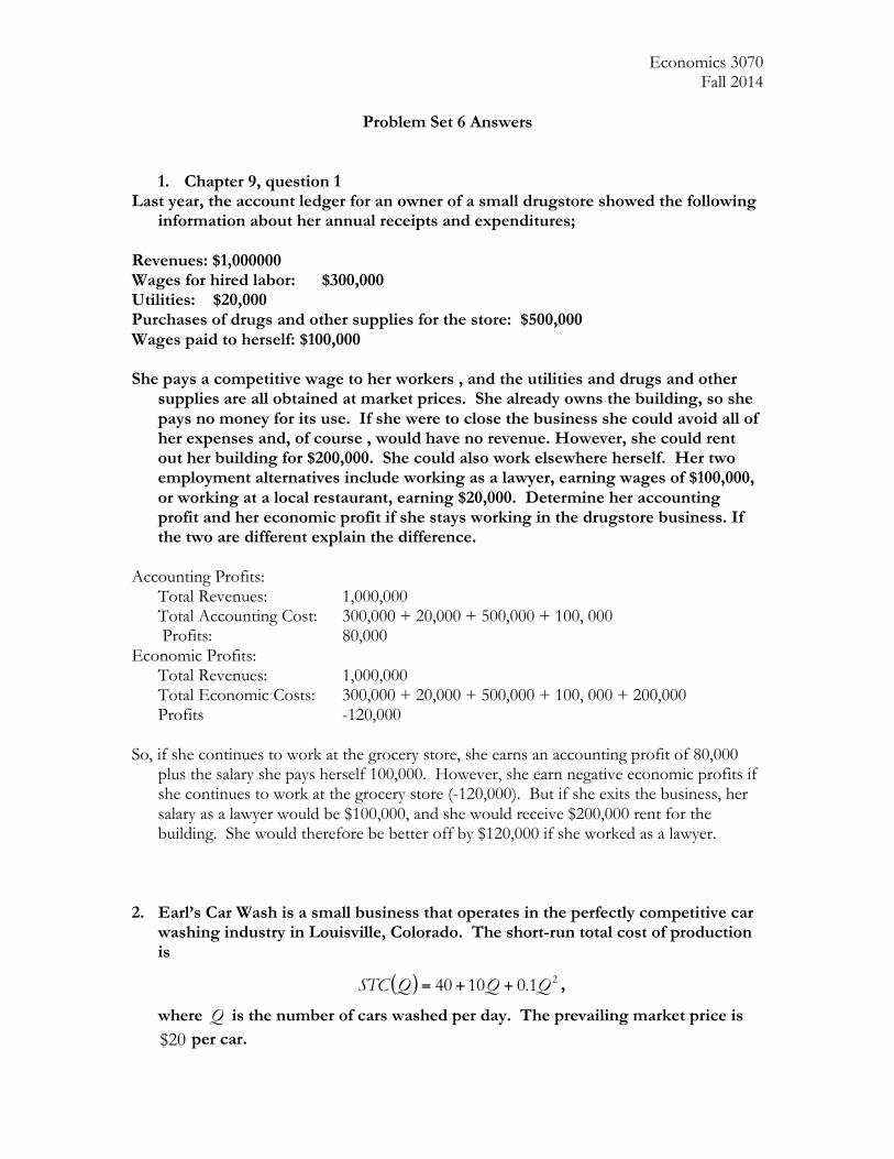
1. Chapter 9, question 1 Last year, the account ledger for an owner of a small drugstore showed the following
information about her annual receipts and expenditures; Revenues: $1,000000 Wages for hired labor: $300,000 Utilities: $20,000 Purchases of drugs and other supplies for the store: $500,000 Wages paid to herself: $100,000 She pays a competitive wage to her workers , and the utilities and drugs and other
supplies are all obtained at market prices. She already owns the building, so she pays no money for its use. If she were to close the business she could avoid all of her expenses and, of course , would have no revenue. However, she could rent out her building for $200,000. She could also work elsewhere herself. Her two employment alternatives include working as a lawyer, earning wages of $100,000, or working at a local restaurant, earning $20,000. Determine her accounting profit and her economic profit if she stays working in the drugstore business. If the two are different explain the difference.
Accounting Profits: Total Revenues: 1,000,000 Total Accounting Cost: 300,000 + 20,000 + 500,000 + 100, 000 Profits: 80,000 Economic Profits: Total Revenues: 1,000,000 Total Economic Costs: 300,000 + 20,000 + 500,000 + 100, 000 + 200,000 Profits -120,000 So, if she continues to work at the grocery store, she earns an accounting profit of 80,000
plus the salary she pays herself 100,000. However, she earn negative economic profits if she continues to work at the grocery store (-120,000). But if she exits the business, her salary as a lawyer would be $100,000, and she would receive $200,000 rent for the building. She would therefore be better off by $120,000 if she worked as a lawyer.
2. Earl’s Car Wash is a small business that operates in the perfectly competitive car
washing industry in Louisville, Colorado. The short-run total cost of production is
( ) 21.01040 QQQSTC ++= ,
where Q is the number of cars washed per day. The prevailing market price is 20$ per car.
Economics 3070 Fall 2014
a. How many cars should Earl wash to maximize profit?
Earl needs to maximize the profit function:
2. (40 10 0.1 )
10 .2 0
10 .2
QMax P Q Q Q
P QQP Q
π
π
= − + +
∂= − − =
∂
= +
If price equals 20 then:
50
2.01020
=
+=
Q
Q
Therefore, Earl should wash 50 cars to maximize profit. b. What is Earl’s maximum daily profit?
Earl’s profit is given by TCTR −=π .
( )( )( ) ( )( ) ( )( )[ ]210
501.05010405020
1.01040
2
2
=
++−=
++−= QQPQπ
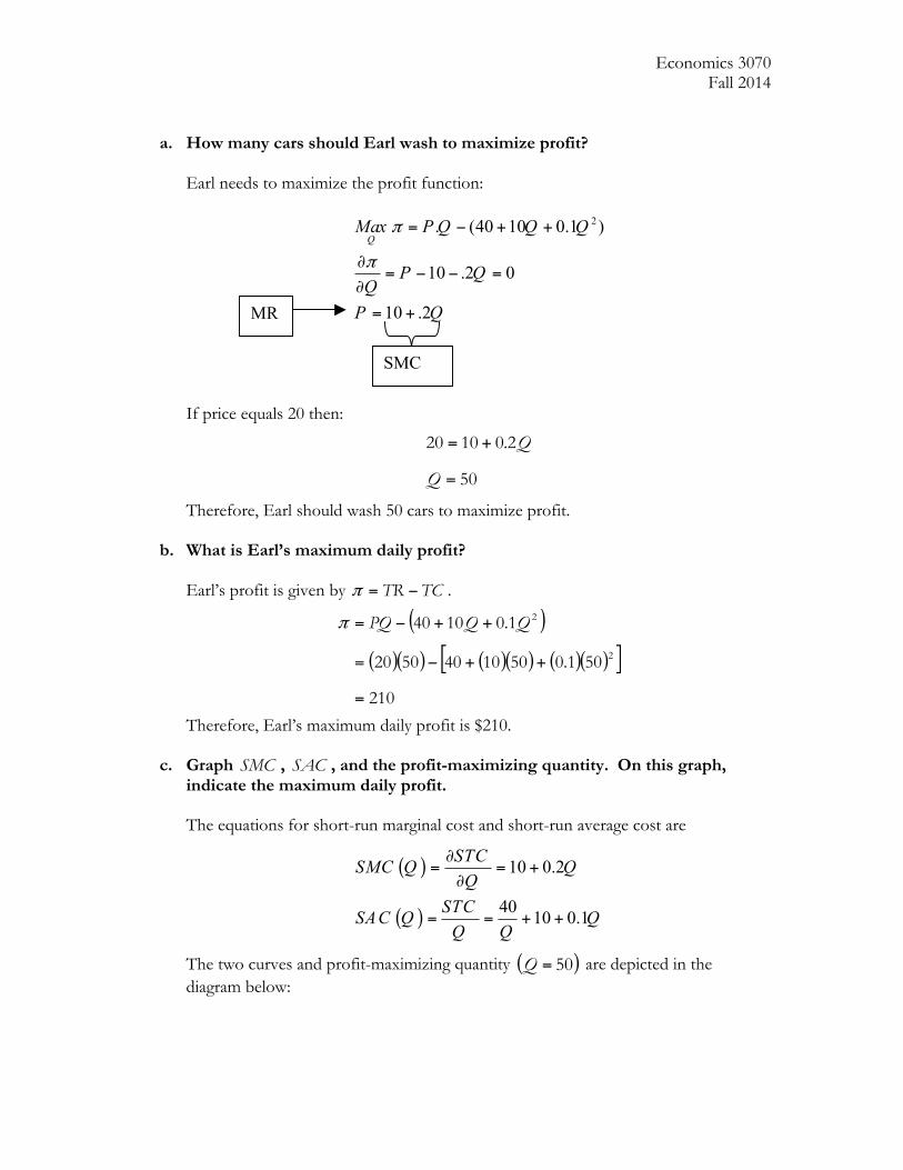
Therefore, Earl’s maximum daily profit is $210. c. Graph SMC , SAC , and the profit-maximizing quantity. On this graph,
indicate the maximum daily profit. The equations for short-run marginal cost and short-run average cost are
( )
( )
10 0.2
40 10 0.1
STCSMC Q QQ
STCSAC Q QQ Q
∂= = +
∂
= = + +
The two curves and profit-maximizing quantity ( )50=Q are depicted in the diagram below:
MR
SMC
Economics 3070 Fall 2014
The shaded area represents the Earl’s profit. It is a rectangle whose height is the difference between the market price ( )20=P and the average cost of the 50th unit
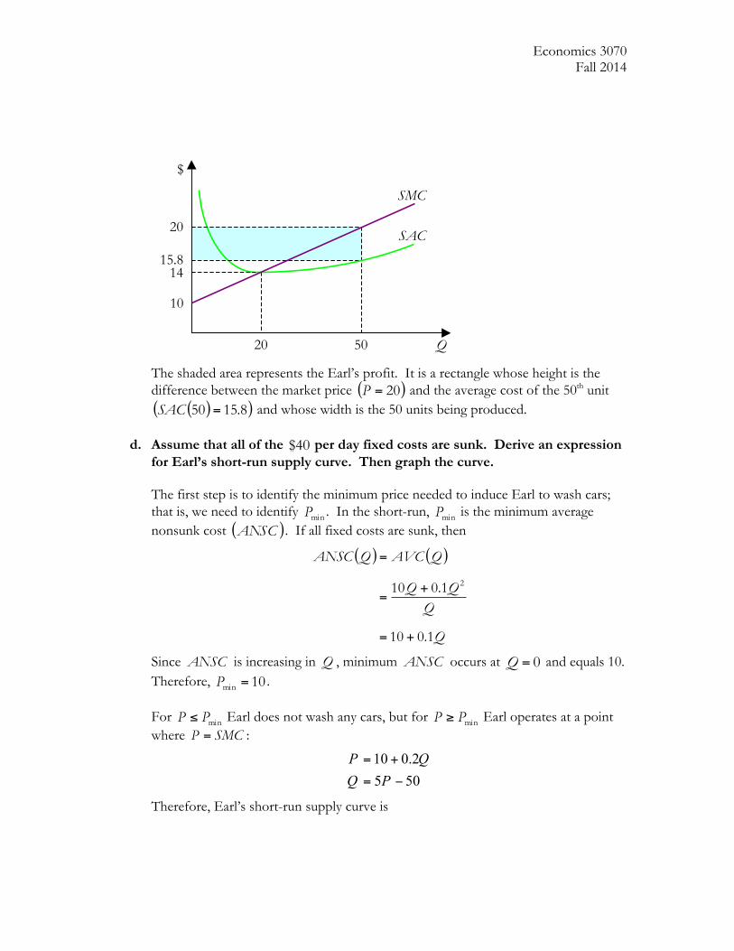
( )( )8.1550 =SAC and whose width is the 50 units being produced. d. Assume that all of the 40$ per day fixed costs are sunk. Derive an expression
for Earl’s short-run supply curve. Then graph the curve.
The first step is to identify the minimum price needed to induce Earl to wash cars; that is, we need to identify minP . In the short-run, minP is the minimum average nonsunk cost ( )ANSC . If all fixed costs are sunk, then
( ) ( )
Q
QQQ
QAVCQANSC
1.010
1.010 2
+=
+=
=
Since ANSC is increasing in Q , minimum ANSC occurs at 0=Q and equals 10. Therefore, 10min =P . For minPP ≤ Earl does not wash any cars, but for minPP ≥ Earl operates at a point where SMCP = :
10 0.25 50
P QQ P= +
= −
Therefore, Earl’s short-run supply curve is
Q
$
SAC
SMC
10
14
20
50 20
15.8
Economics 3070 Fall 2014
( )⎪⎩
⎪⎨⎧
≥−
≤=
10 if505
10 if0
PP
PPs
The graph below depicts this supply curve:
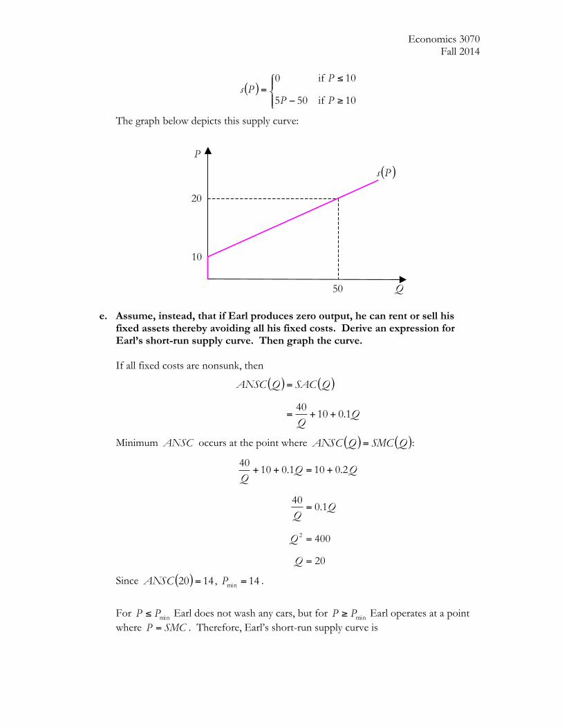
e. Assume, instead, that if Earl produces zero output, he can rent or sell his
fixed assets thereby avoiding all his fixed costs. Derive an expression for Earl’s short-run supply curve. Then graph the curve. If all fixed costs are nonsunk, then
( ) ( )
QSACQANSC
1.01040
++=
=
Minimum ANSC occurs at the point where ( ) ( )QSMCQANSC = :
20
400
1.040
2.0101.01040
2
=
=
=
+=++
Q
Q
QQQ
Since ( ) 1420 =ANSC , 14min =P .
For minPP ≤ Earl does not wash any cars, but for minPP ≥ Earl operates at a point where SMCP = . Therefore, Earl’s short-run supply curve is
Q
P
( )Ps
10
20
50
Economics 3070 Fall 2014
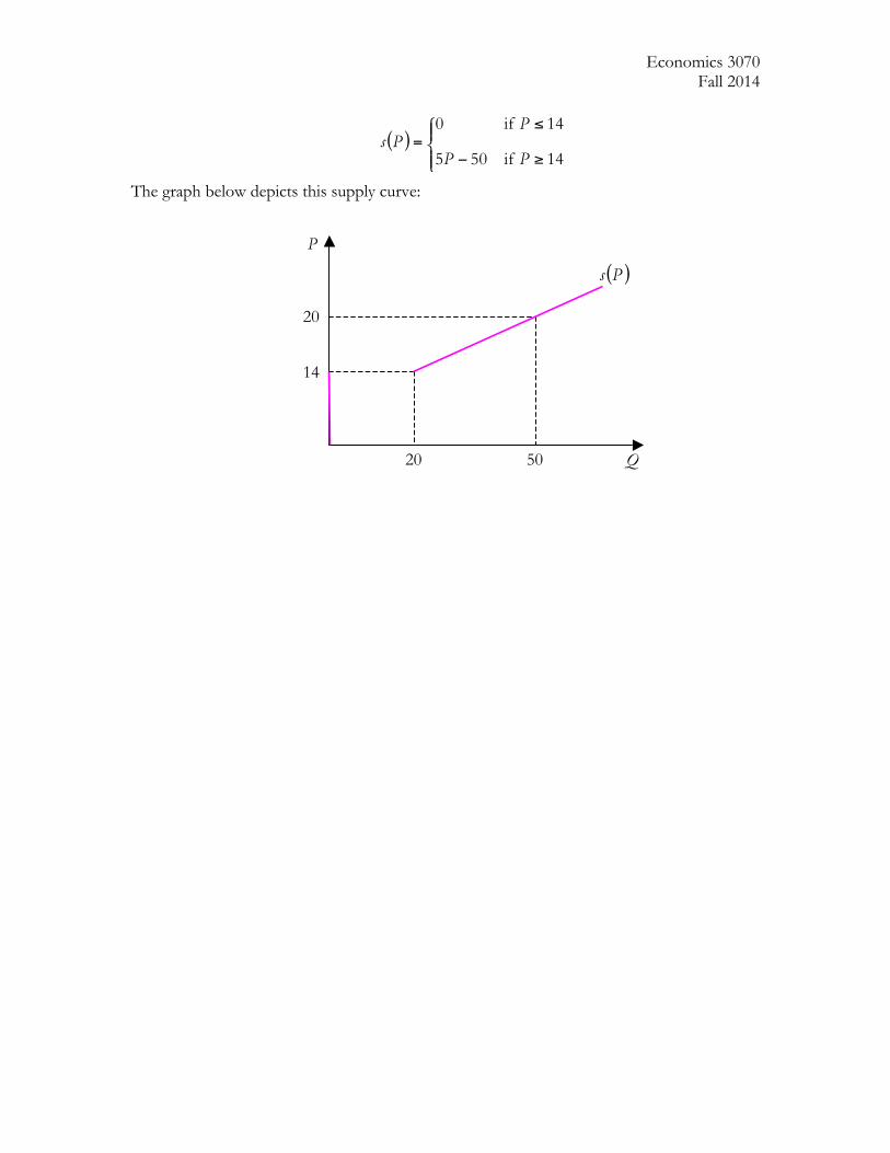
( )⎪⎩
⎪⎨⎧
≥−
≤=
14 if505
14 if0
PP
PPs
The graph below depicts this supply curve:
Q
P
( )Ps
14
20
50 20
Economics 3070 Fall 2014
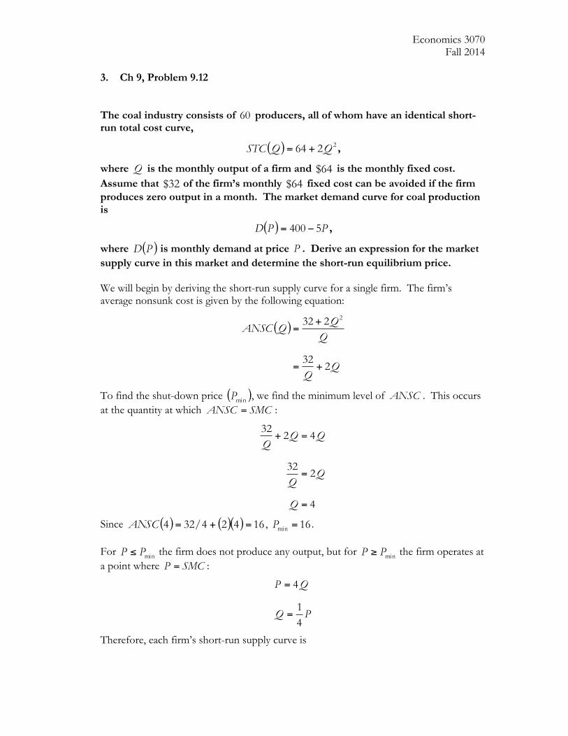
3. Ch 9, Problem 9.12 The coal industry consists of 60 producers, all of whom have an identical short-
run total cost curve,
( ) 2264 QQSTC += ,
where Q is the monthly output of a firm and 64$ is the monthly fixed cost. Assume that 32$ of the firm’s monthly 64$ fixed cost can be avoided if the firm produces zero output in a month. The market demand curve for coal production is
( ) PPD 5400 −= ,
where ( )PD is monthly demand at price P . Derive an expression for the market supply curve in this market and determine the short-run equilibrium price. We will begin by deriving the short-run supply curve for a single firm. The firm’s average nonsunk cost is given by the following equation:
( )
QANSC
232
232 2
+=
+=
To find the shut-down price ( )minP , we find the minimum level of ANSC . This occurs at the quantity at which SMCANSC = :
4
232
4232
=
=
=+
Q
QQQ
Since ( ) ( )( ) 16424/324 =+=ANSC , 16min =P . For minPP ≤ the firm does not produce any output, but for minPP ≥ the firm operates at a point where SMCP = :
PQ
QP
41
4
=
=
Therefore, each firm’s short-run supply curve is
Economics 3070 Fall 2014
( )⎪⎩
⎪⎨⎧
≥
≤=
16 if
16 if0
41 PP
PPs
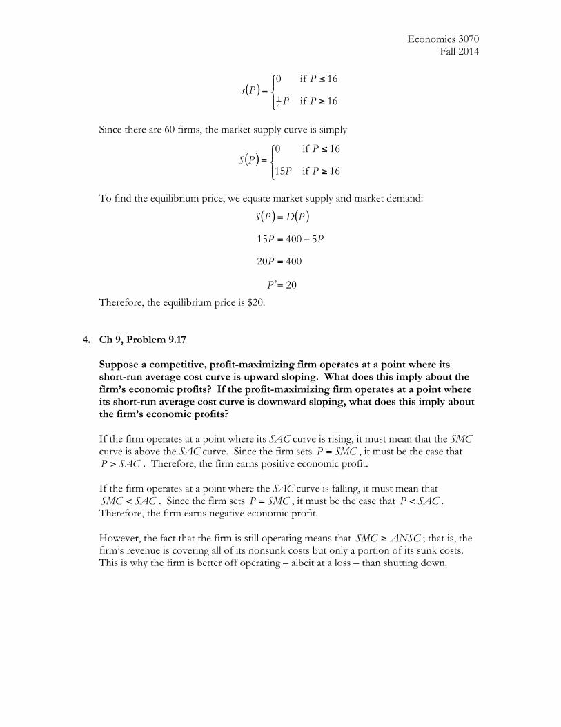
Since there are 60 firms, the market supply curve is simply
( )⎪⎩
⎪⎨⎧
≥
≤=
16 if15
16 if0
PP
PPS
To find the equilibrium price, we equate market supply and market demand:
( ) ( )
20
40020
540015
=
=
−=
=
∗P
P
PP
PDPS
Therefore, the equilibrium price is $20. 4. Ch 9, Problem 9.17
Suppose a competitive, profit-maximizing firm operates at a point where its short-run average cost curve is upward sloping. What does this imply about the firm’s economic profits? If the profit-maximizing firm operates at a point where its short-run average cost curve is downward sloping, what does this imply about the firm’s economic profits? If the firm operates at a point where its SAC curve is rising, it must mean that the SMC curve is above the SAC curve. Since the firm sets SMCP = , it must be the case that
SACP > . Therefore, the firm earns positive economic profit. If the firm operates at a point where the SAC curve is falling, it must mean that
SACSMC < . Since the firm sets SMCP = , it must be the case that SACP < . Therefore, the firm earns negative economic profit. However, the fact that the firm is still operating means that ANSCSMC ≥ ; that is, the firm’s revenue is covering all of its nonsunk costs but only a portion of its sunk costs. This is why the firm is better off operating – albeit at a loss – than shutting down.
Economics 3070 Fall 2014
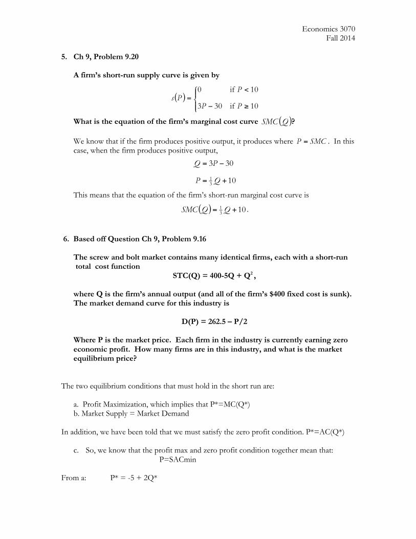
5. Ch 9, Problem 9.20 A firm’s short-run supply curve is given by
( )⎪⎩
⎪⎨⎧
≥−
<=
10 if303
10 if0
PP
PPs
What is the equation of the firm’s marginal cost curve ( )QSMC ? We know that if the firm produces positive output, it produces where SMCP = . In this case, when the firm produces positive output,
10
303
31 +=
−=
QP
PQ
This means that the equation of the firm’s short-run marginal cost curve is
( ) 1031 += QQSMC .
6. Based off Question Ch 9, Problem 9.16 The screw and bolt market contains many identical firms, each with a short-run total cost function
STC(Q) = 400-5Q + Q2 , where Q is the firm’s annual output (and all of the firm’s $400 fixed cost is sunk). The market demand curve for this industry is
D(P) = 262.5 – P/2
Where P is the market price. Each firm in the industry is currently earning zero economic profit. How many firms are in this industry, and what is the market equilibrium price?
The two equilibrium conditions that must hold in the short run are: a. Profit Maximization, which implies that P*=MC(Q*) b. Market Supply = Market Demand In addition, we have been told that we must satisfy the zero profit condition. P*=AC(Q*)
c. So, we know that the profit max and zero profit condition together mean that: P=SACmin From a: P* = -5 + 2Q*
Economics 3070 Fall 2014
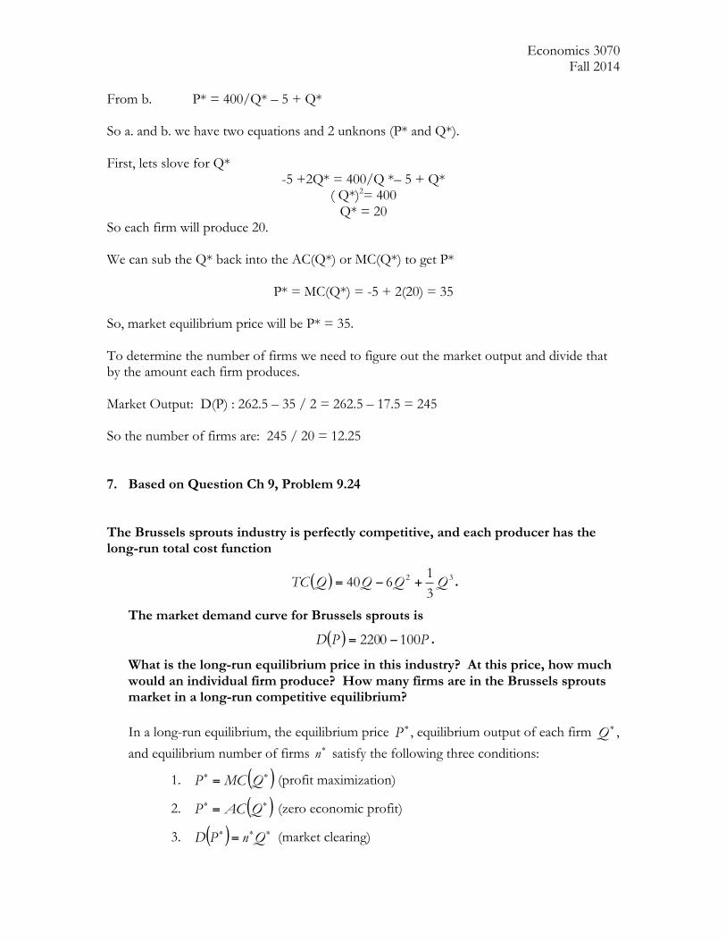
From b. P* = 400/Q* – 5 + Q* So a. and b. we have two equations and 2 unknons (P* and Q*). First, lets slove for Q*
-5 +2Q* = 400/Q *– 5 + Q* ( Q*)2= 400
Q* = 20 So each firm will produce 20.
We can sub the Q* back into the AC(Q*) or MC(Q*) to get P*
P* = MC(Q*) = -5 + 2(20) = 35 So, market equilibrium price will be P* = 35. To determine the number of firms we need to figure out the market output and divide that by the amount each firm produces. Market Output: D(P) : 262.5 – 35 / 2 = 262.5 – 17.5 = 245 So the number of firms are: 245 / 20 = 12.25 7. Based on Question Ch 9, Problem 9.24 The Brussels sprouts industry is perfectly competitive, and each producer has the long-run total cost function
( ) 32
31
640 QQQQTC +−= .
The market demand curve for Brussels sprouts is
( ) PPD 1002200 −= .
What is the long-run equilibrium price in this industry? At this price, how much would an individual firm produce? How many firms are in the Brussels sprouts market in a long-run competitive equilibrium? In a long-run equilibrium, the equilibrium price ∗P , equilibrium output of each firm ∗Q ,
and equilibrium number of firms ∗n satisfy the following three conditions:
1. ( )∗∗ = QMCP (profit maximization)
2. ( )∗∗ = QACP (zero economic profit)
3. ( ) ∗∗∗ = QnPD (market clearing)

Economics 3070 Fall 2014
The first step is to apply conditions 1 and 2 by setting ( ) ( )∗∗ = QACQMC :
9
182
6
6401240
2
232
2312
=
=
=
+−=+−
∗Q
QQQQ
Therefore, each individual firm produces 9=∗Q units of Brussels sprouts. To find the equilibrium price, we simply plug 9=∗Q into ( )∗QMC :
( ) ( ) ( )
13
8110840
9912409 2
=
+−=
+−=MC
Therefore, the long-run equilibrium price is 13=∗P . To find the equilibrium number of firms, we apply condition 2 by plugging 13=∗P into the market demand curve:
( )
( ) ( )( )
( )
100
9009
13002200
13100220013
1002200
=
=
−=
−=
−=
∗
∗
∗∗
n
n
Qn
D
PPD
Therefore, the equilibrium number of firms is 100=∗n . 8. Based on Question Ch 9, Problem 9.32 The long-run total cost for production of exam booklets is given by
2 3(120 20 )TC wr Q Q Q= − + ,
Where Q is the annual output of a firm, w is the wage rate for skilled assembly labor, and r is the price of capital services. The demand for labor for an individual firm is
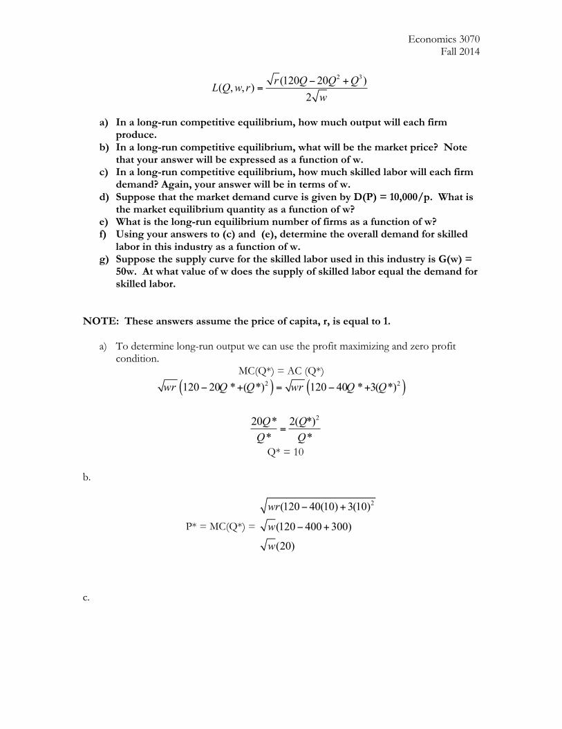
Economics 3070 Fall 2014
2 3(120 20 )( , , )2
r Q Q QL Q w rw
− +=
a) In a long-run competitive equilibrium, how much output will each firm
produce. b) In a long-run competitive equilibrium, what will be the market price? Note
that your answer will be expressed as a function of w. c) In a long-run competitive equilibrium, how much skilled labor will each firm
demand? Again, your answer will be in terms of w. d) Suppose that the market demand curve is given by D(P) = 10,000/p. What is
the market equilibrium quantity as a function of w? e) What is the long-run equilibrium number of firms as a function of w? f) Using your answers to (c) and (e), determine the overall demand for skilled
labor in this industry as a function of w. g) Suppose the supply curve for the skilled labor used in this industry is G(w) =
50w. At what value of w does the supply of skilled labor equal the demand for skilled labor.
NOTE: These answers assume the price of capita, r, is equal to 1.
a) To determine long-run output we can use the profit maximizing and zero profit condition.
MC(Q*) = AC (Q*)
( ) ( )2 2120 20 * ( *) 120 40 * 3( *)wr Q Q wr Q Q− + = − +
220 * 2( *)* *Q QQ Q
=
Q* = 10
b.
P* = MC(Q*) =
2(120 40(10) 3(10)
(120 400 300)
(20)
wr
w
w
− +
− +
c.

Economics 3070 Fall 2014
2 3120*10 20*10 10( , , )2
200 1002
L Q w rw
w w
− +=
= =

Economics 3070 Fall 2014
d.
10,000 10,000 500( *)* 20
D PP w w
= = =
e.
500( *) 50** 10
D P wnQ w
= = =
f. Demand for skilled labor: Demand for Lobor by each firm * number of firms.
100 50 5000*w w w
=
g.
2
5000 50
10010
L LD S
wwww
=
=
=
=