Economics 310

Lecture 27Distributed Lag Models

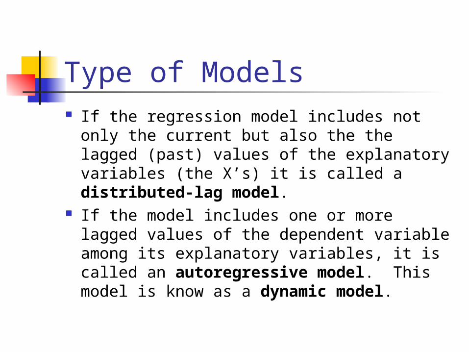
Type of Models If the regression model includes not only

the current but also the the lagged (past) values of the explanatory variables (the X’s) it is called a distributed-lag model.

If the model includes one or more lagged values of the dependent variable among its explanatory variables, it is called an autoregressive model. This model is know as a dynamic model.

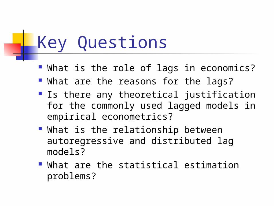
Key Questions What is the role of lags in economics? What are the reasons for the lags? Is there any theoretical justification for the

commonly used lagged models in empirical econometrics?

What is the relationship between autoregressive and distributed lag models?

What are the statistical estimation problems?

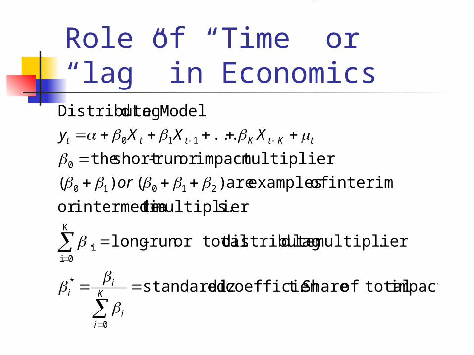
Role of “Time” or “lag” in Economics

impact. totalof Share t.coefficien edstandardiz

.multiplier lag ddistribute or totalrun -long.

s.multiplier teintermediaor

interim of examples are )()(

multiplierimpact or run -short the

...

Model Lag dDistribute

0

*

K

0ii

21010

0

110

K

ii

ii

tKtKttt

or

XXXy

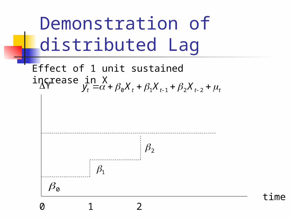
Demonstration of distributed Lag

Effect of 1 unit sustained increase in X

time

Y

0 1 2

ttttt XXXy 22110

01

2

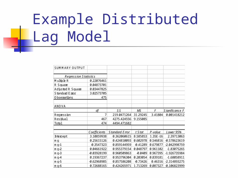
Example Distributed Lag Model

SUMMARY OUTPUT

Regression StatisticsMultiple R 0.22076461R Square 0.04873701Adjusted R Square 0.03447825Standard Error 3.02573705Observations 475

ANOVAdf SS MS F Significance F

Regression 7 219.0471264 31.29245 3.41804 0.001418212Residual 467 4275.424556 9.155085Total 474 4494.471682

Coefficients Standard Error t Stat P-value Lower 95%Intercept 3.10859938 0.362060615 8.585853 1.35E-16 2.39713063mg 0.25615126 0.424810093 0.602978 0.546816 -0.578623619mg-1 -0.3547323 0.859144959 -0.41289 0.679877 -2.042998759mg-2 0.04661922 0.955379154 0.048797 0.961102 -1.83075265mg-3 -0.03928199 0.960509863 -0.0409 0.967395 -1.926735984mg-4 0.19367237 0.953796304 0.203054 0.839181 -1.68058911mg-5 -0.62968985 0.857586208 -0.73426 0.46316 -2.314893275mg-6 0.72688165 0.424265971 1.713269 0.087327 -0.106823999

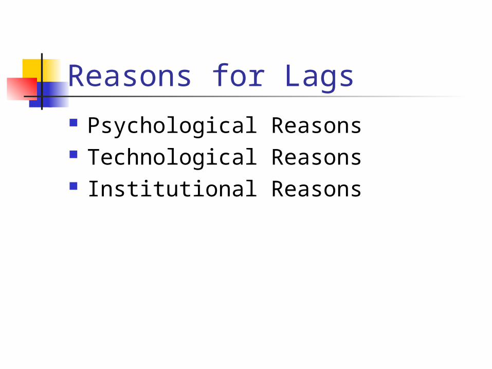
Reasons for Lags Psychological Reasons Technological Reasons Institutional Reasons

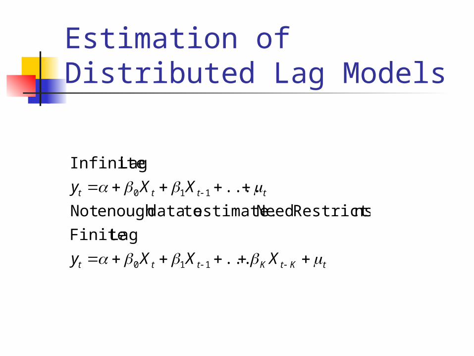
Estimation of Distributed Lag Models

tKtKttt

tttt

XXXy

XXy

...

Lag Finite

nsRestrictio Need estimate. todataenough Not

....

Lag Infinite

110

110

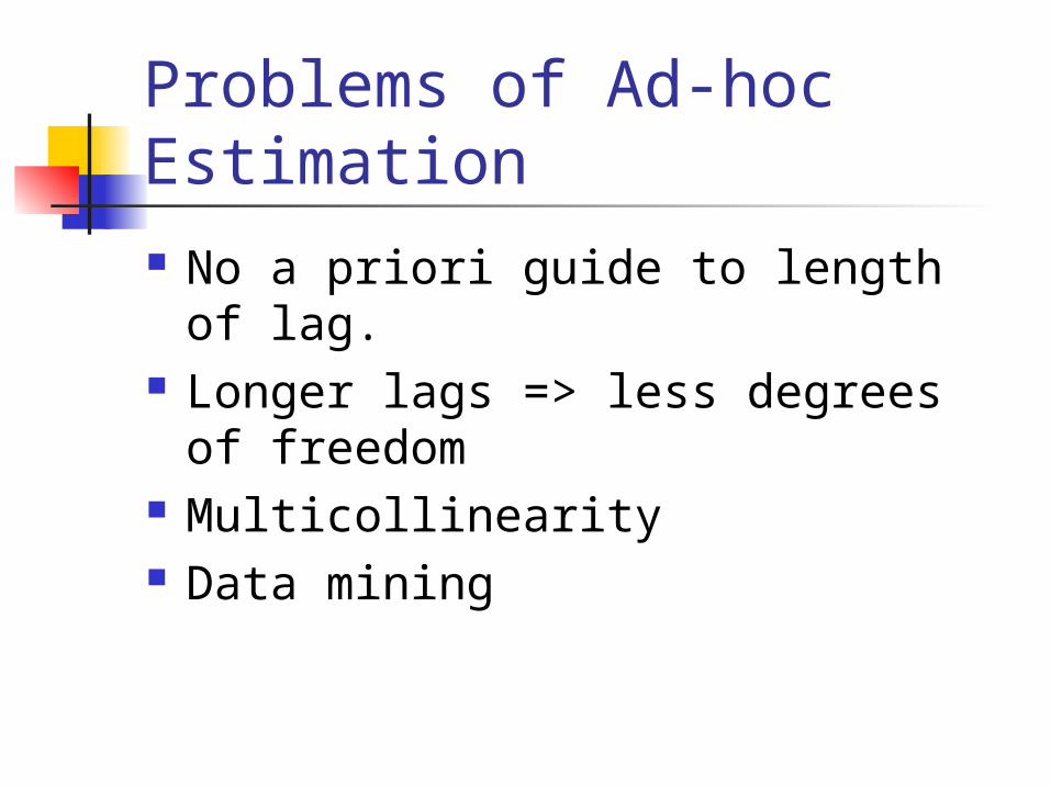
Problems of Ad-hoc Estimation No a priori guide to length of lag. Longer lags => less degrees of

freedom Multicollinearity Data mining

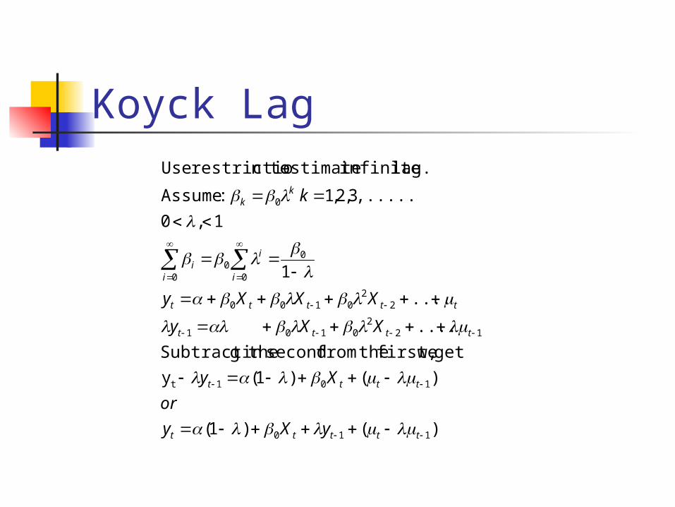
Koyck Lag

)()1(

)()1(y

get wefirst, thefrom second thegSubtractin

....

....

1

1,0

,.....3,2,1 :Assume

lag. infinite estimate tonrestrictio Use

110

101t

122

0101

22

0100

0

0

00

0

ttttt

tttt

tttt

ttttt

i

i

ii

kk

yXy

or

Xy

XXy

XXXy

k

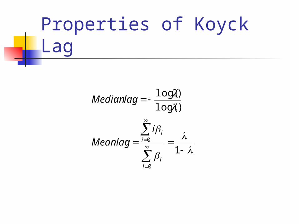
Properties of Koyck Lag

1

)log(

)2log(

0

0

ii

iii

lagMean

lagMedian

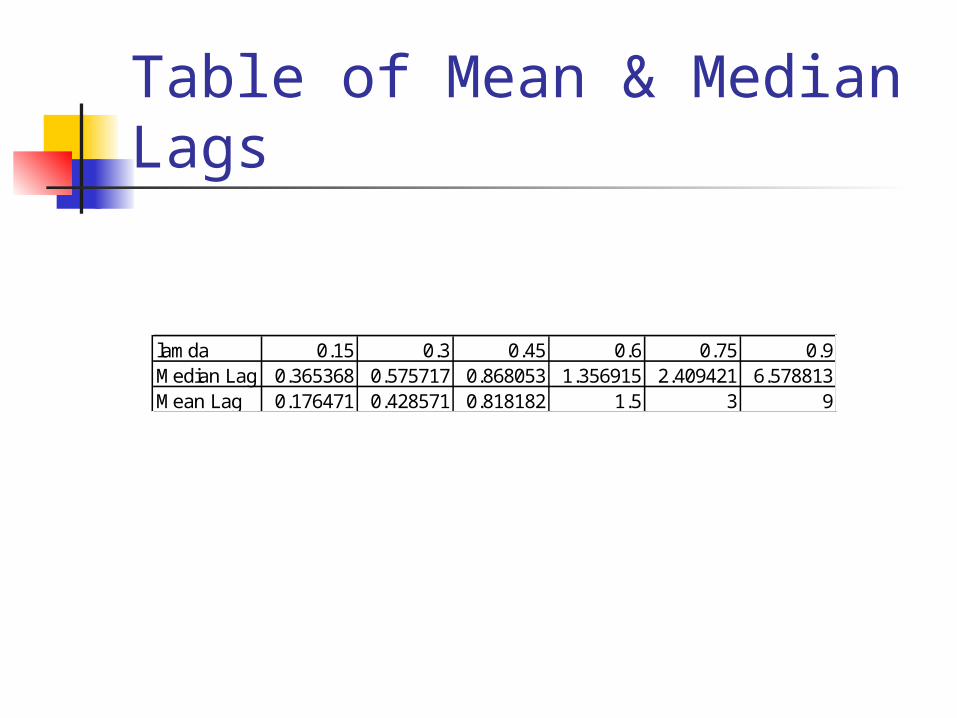
Table of Mean & Median Lags

lamda 0.15 0.3 0.45 0.6 0.75 0.9Median Lag 0.365368 0.575717 0.868053 1.356915 2.409421 6.578813Mean Lag 0.176471 0.428571 0.818182 1.5 3 9

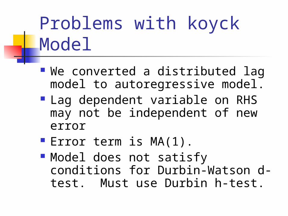
Problems with koyck Model We converted a distributed lag

model to autoregressive model. Lag dependent variable on RHS may

not be independent of new error Error term is MA(1). Model does not satisfy conditions for

Durbin-Watson d-test. Must use Durbin h-test.

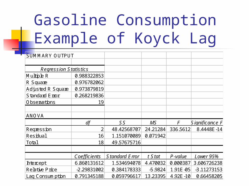
Gasoline Consumption Example of Koyck Lag

SUMMARY OUTPUT

Regression StatisticsMultiple R 0.988322853R Square 0.976782062Adjusted R Square 0.973879819Standard Error 0.268219836Observations 19

ANOVAdf SS MS F Significance F

Regression 2 48.42568707 24.21284 336.5612 8.4448E-14Residual 16 1.151070089 0.071942Total 18 49.57675716

Coefficients Standard Error t Stat P-value Lower 95%Intercept 6.860131612 1.534694078 4.470032 0.000387 3.606726238Relative Price -2.29831002 0.384178333 -5.9824 1.91E-05 -3.11273153Lag Consumption 0.791345188 0.059796617 13.23395 4.92E-10 0.66458205

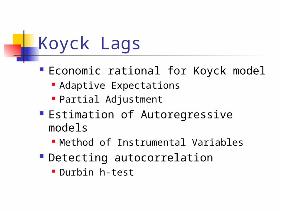
Koyck Lags Economic rational for Koyck model

Adaptive Expectations Partial Adjustment

Estimation of Autoregressive models Method of Instrumental Variables

Detecting autocorrelation Durbin h-test

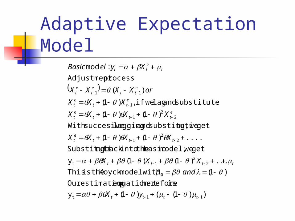
Adaptive Expectation Model

))1(()1(y

is hereforeequation t estimatingOur

)1( with modelKoyck theis This

...)1()1(y

get wemodel, basic theintoback ngSubstituti

....)1()1(

get weng,substituti and lagging succesiveWith

)1()1(

substitute and lag weif ,)1(

)(

process Adjustment

:mod

11t

0

22

1t

22

1

22

1

1

11

tttt

tttt

tttet

ettt

et

ett

et

ett

et

et

tett

yX

and

XXX

XXXX

XXXX

XXX

orXXXX

XyelBasic

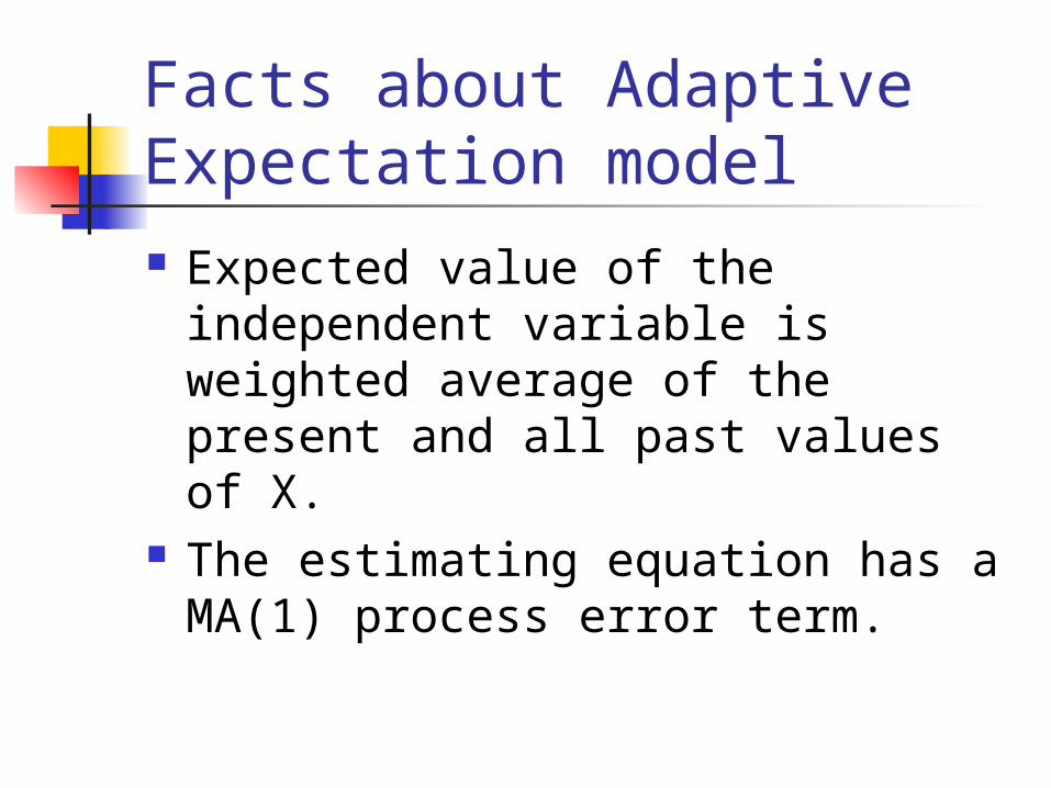
Facts about Adaptive Expectation model Expected value of the independent

variable is weighted average of the present and all past values of X.

The estimating equation has a MA(1) process error term.

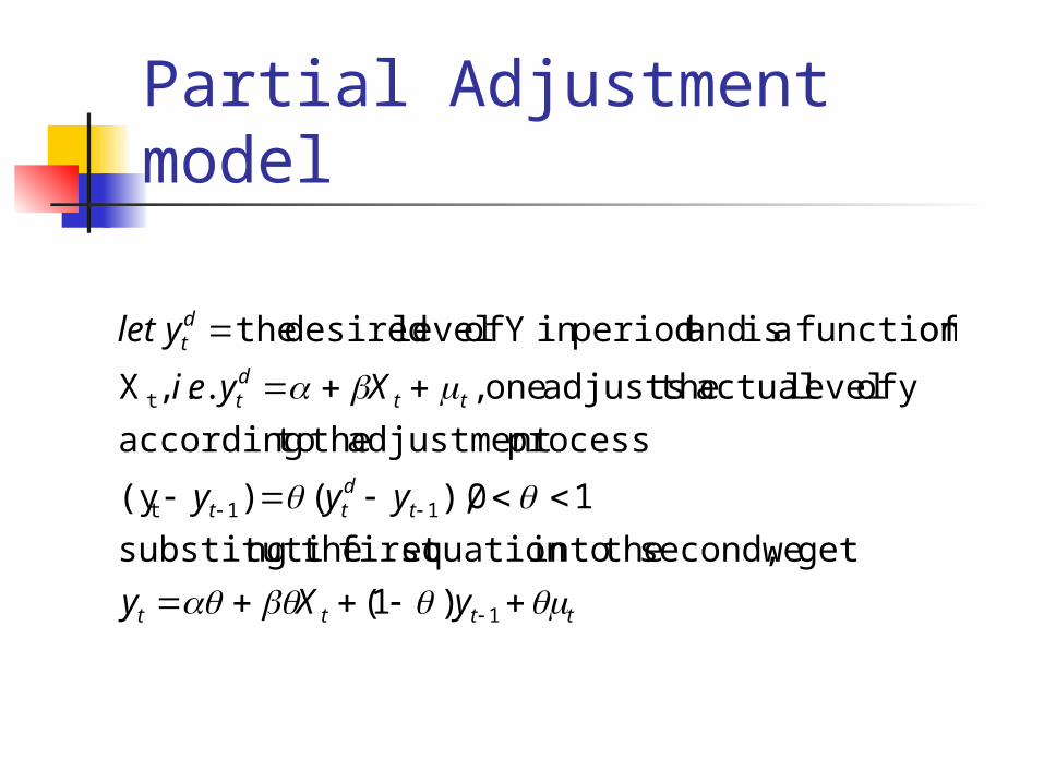
Partial Adjustment model

tttt

tdtt

ttdt

dt

yXy

yyy

Xyei

ylet

1

11t

t

)1(

get wesecond, theintoequation first thengsubstituti

10),()(y

process adjustment the toaccording

y of level actual theadjusts one ,..,X

offunction a is and t periodin Y of level desired the

Properties of partial adjustment model Estimating equation looks like Koyck but

is different as far as estimation is concerned

Error term is well behaved In the limit the lagged dependent

variable is uncorrelated with the error term

model can be estimated consistently by OLS

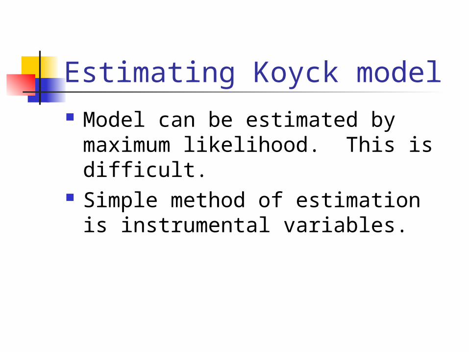
Estimating Koyck model Model can be estimated by

maximum likelihood. This is difficult.

Simple method of estimation is instrumental variables.

Instrumental Variable Estimation

12101

11-t

1-t

t

t

ˆ

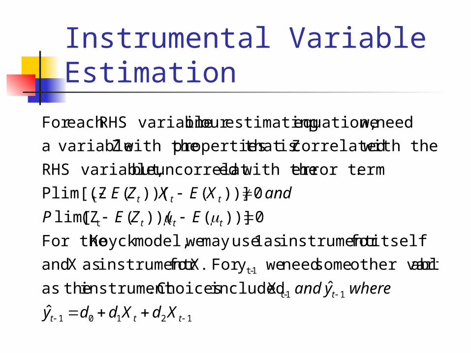
ˆX included Choices .instrument theas

ableother vari some need weyFor X.for instrument as X and

itselffor instrument as 1 usemay wemodel,Koyck For the

0))]())(((Zlim[

0))]())((Plim[(Z

.error term with theeduncorrelatbut variable,RHS

with thecorrelated is that Zproperties with the Z variablea

need weequation, estimatingour in variableRHSeach For

ttt

t

ttt

ttt

XdXddy

whereyand

EZEP

andXEXZE

Instrumental Variable Estimation Continued

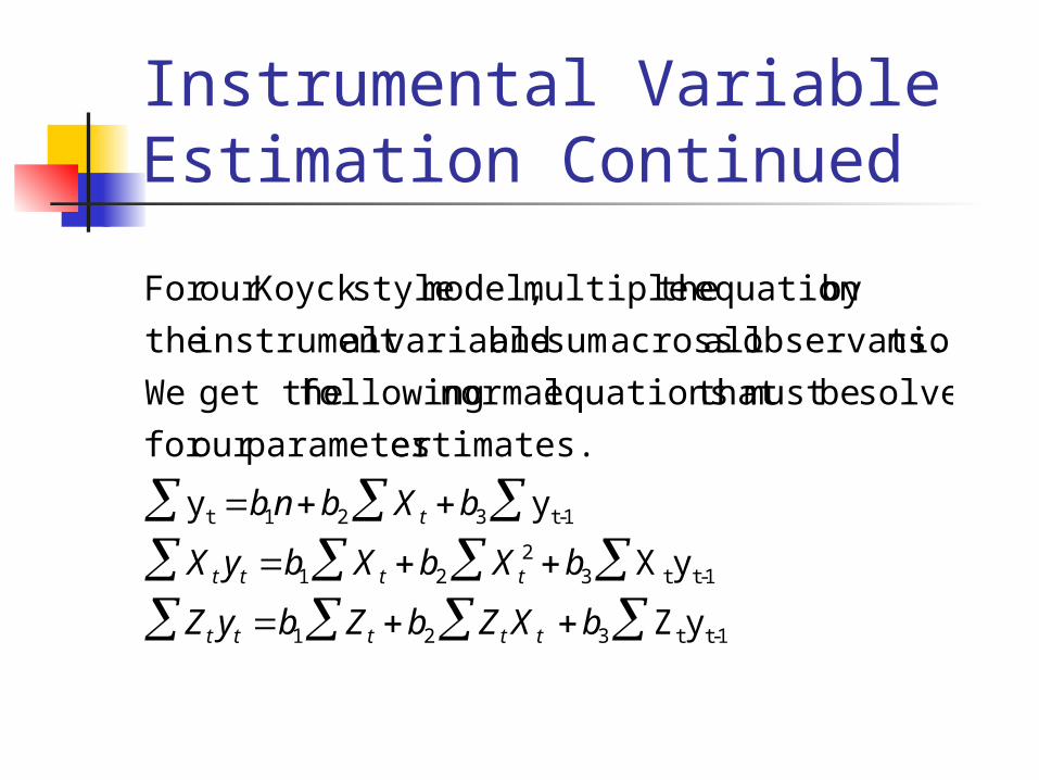
1-tt321

1-tt32

21

1-t321t

yZ

yX

yy

estimates.parameter our for

solved bemust that equations normal following get the We

ns.observatio all across sum and variablealinstrument the

byequation themultiple model, styleKoyck our For

bXZbZbyZ

bXbXbyX

bXbnb

ttttt

tttt

t

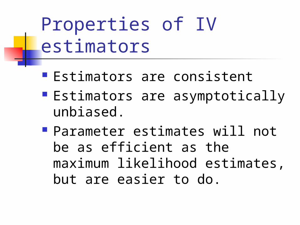
Properties of IV estimators Estimators are consistent Estimators are asymptotically

unbiased. Parameter estimates will not be as

efficient as the maximum likelihood estimates, but are easier to do.

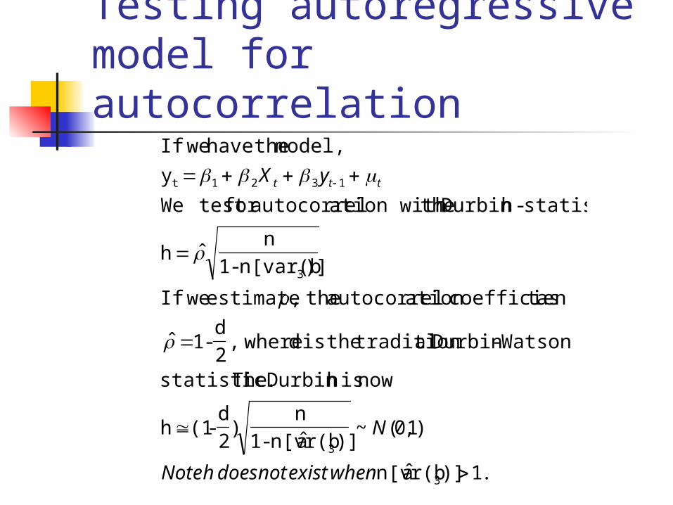
Testing autoregressive model for autocorrelation

.1)]r(ban[v

)1,0(~)]r(ban[v-1

n)

2

d-(1h

now ish Durbin The statistic.

Watson-Durbin al tradition theis d where,2

d-1ˆ

ast coefficienation autocorrel the, estimate weIf

)]n[var(b-1

nˆh

statistic-hDurbin theation withautocorrelfor test We

y

model, thehave weIf

3

3

3

1321t

whenexistnotdoeshNote

N

yX ttt

Adaptive expectations example

))1((t)Investmen-(1

)1(

))1(1(by through gmultiplyin

))1(1(

))1(1(

ithequation wfirst in theinterest expected replaced

..,

))1(1(

)()(

1t1-t

1221

21

1

11

21

t

tttt

ttt

t

tet

tt

tet

ett

et

et

ttett

salessalesInterestInvestment

givesL

SalesL

InterestInvestment

givesL

InterestInterest

xLxeioperatorlagLWhere

InterestInterestL

InterestInterestInterestInterest

SalesInterestInvestment

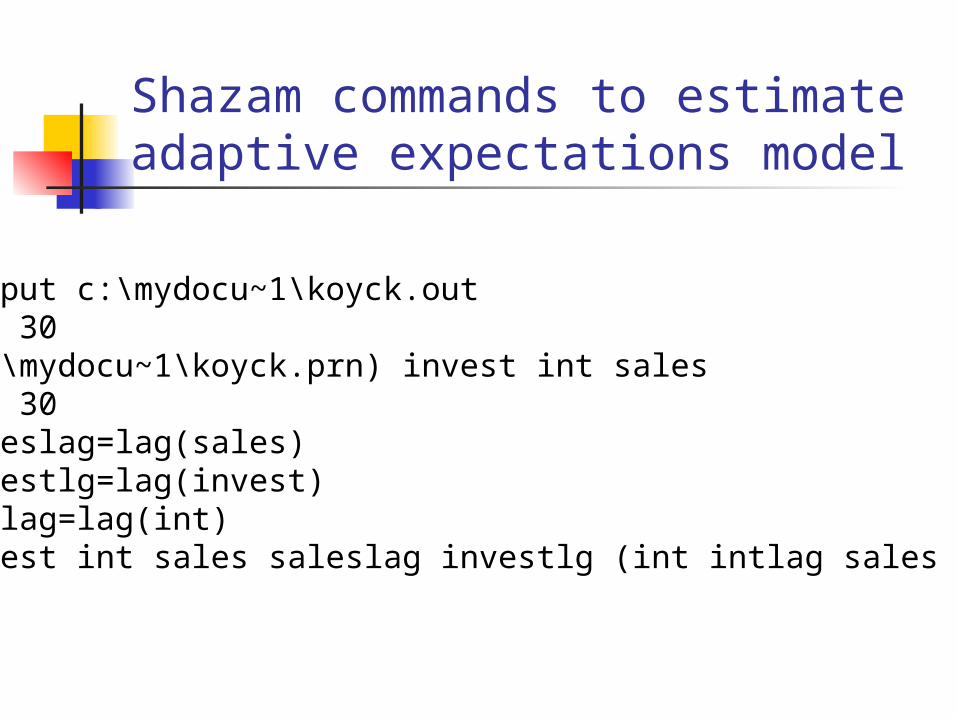
Shazam commands to estimate adaptive expectations model

file output c:\mydocu~1\koyck.outsample 1 30read (c:\mydocu~1\koyck.prn) invest int salessample 2 30genr saleslag=lag(sales)genr investlg=lag(invest)genr intlag=lag(int)inst invest int sales saleslag investlg (int intlag sales saleslag)stop

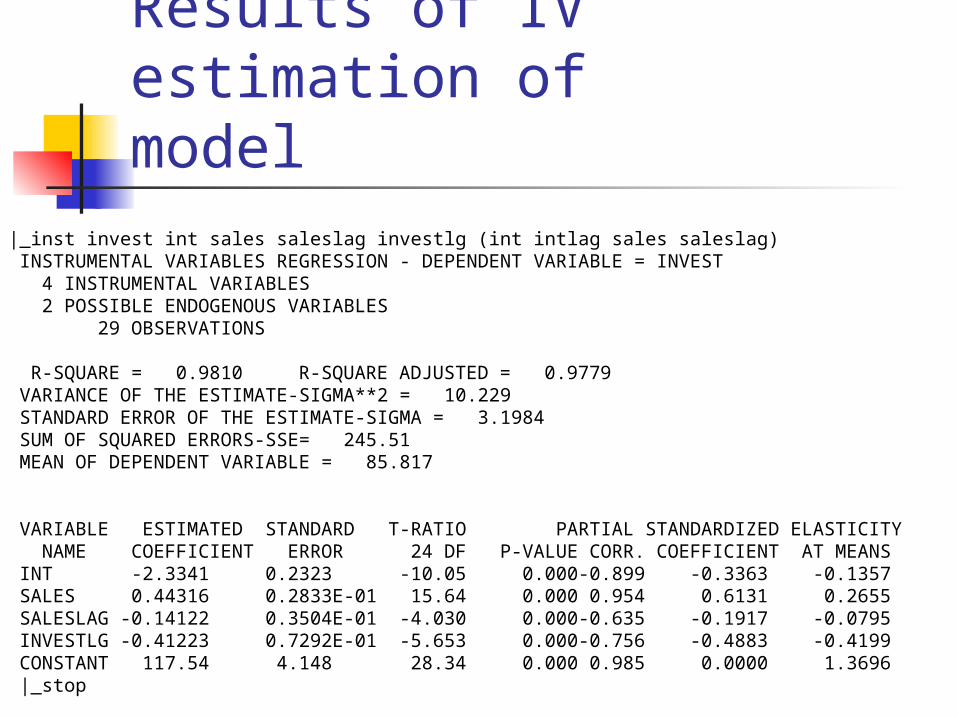
Results of IV estimation ofmodel

|_inst invest int sales saleslag investlg (int intlag sales saleslag) INSTRUMENTAL VARIABLES REGRESSION - DEPENDENT VARIABLE = INVEST 4 INSTRUMENTAL VARIABLES 2 POSSIBLE ENDOGENOUS VARIABLES 29 OBSERVATIONS R-SQUARE = 0.9810 R-SQUARE ADJUSTED = 0.9779 VARIANCE OF THE ESTIMATE-SIGMA**2 = 10.229 STANDARD ERROR OF THE ESTIMATE-SIGMA = 3.1984 SUM OF SQUARED ERRORS-SSE= 245.51 MEAN OF DEPENDENT VARIABLE = 85.817 VARIABLE ESTIMATED STANDARD T-RATIO PARTIAL STANDARDIZED ELASTICITY NAME COEFFICIENT ERROR 24 DF P-VALUE CORR. COEFFICIENT AT MEANS INT -2.3341 0.2323 -10.05 0.000-0.899 -0.3363 -0.1357 SALES 0.44316 0.2833E-01 15.64 0.000 0.954 0.6131 0.2655 SALESLAG -0.14122 0.3504E-01 -4.030 0.000-0.635 -0.1917 -0.0795 INVESTLG -0.41223 0.7292E-01 -5.653 0.000-0.756 -0.4883 -0.4199 CONSTANT 117.54 4.148 28.34 0.000 0.985 0.0000 1.3696 |_stop

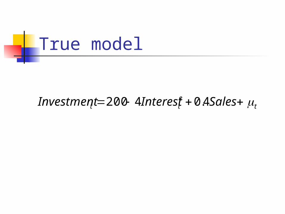
True model

tett SalesInterestInvestment 4.04200