Embed Size (px)
Citation preview

Economics 310Price Theory
Chapters 5 and 6.
Department of Economics
College of Business and Economics
California State University-Northridge
Professor Kenneth Ng
Wednesday, April 19, 2023

The Behavior of Firms. In Chapter 5 and 6 will take a detailed look at the Supply Curve,
i.e. production decision. – Want to answer the question, “ at any given price, how much
will a firm produce and why?”

Efficient production in the multiple input case. If a firm is going to produce a certain
quantity of a good, what is the best, i.e. most efficient method of production.
Consider the two input case, where two inputs, capital and labor are used to produce a given quantity of a good.
Will use two theoretical constructs—iso-cost curve and iso-output curve.
Iso Cost Curves
An isocost curve shows combinations of two inputs (labor and capital) that can be purchased for a given amount.
Similar to a budget line from the discussion about consumer behavior.
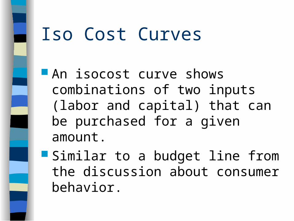
Isocost Curve: $10,000 budget, Price of Labor =$50, Price of Capital=$25
Labor
Capital
0
400
200
$10,000
Any combination of inputs on the iso-cost curve can be purchased for $10,000.

Position of the Isocost curve represents Total Cost: Consider an increase in expenditures on inputs to $15,000. How will this shift the iso-cost curve?
Labor
Capital
0
400
200
$15,000$10,000
300
600 A parallel shift in the isocost curve represents and increase in total cost.
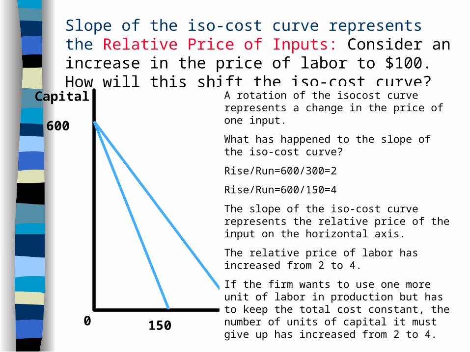
Slope of the iso-cost curve represents the Relative Price of Inputs: Consider an increase in the price of labor to $100. How will this shift the iso-cost curve?
Labor
Capital
0
$15,000
300
600
A rotation of the isocost curve represents a change in the price of one input.
What has happened to the slope of the iso-cost curve?
Rise/Run=600/300=2
Rise/Run=600/150=4
The slope of the iso-cost curve represents the relative price of the input on the horizontal axis.
The relative price of labor has increased from 2 to 4.
If the firm wants to use one more unit of labor in production but has to keep the total cost constant, the number of units of capital it must give up has increased from 2 to 4. 150

Iso output Curves An iso-output curve shows
combinations of two inputs (labor and capital) that produce the same amount of the good.
Similar to an indifference curve from consumer choice discussion.

Movement along the iso-output curve represents a change in the way goods are produced.
Labor
Capital
0
100 Units
A
At points A and B, the firm is producing 100 units of the good but in different ways.
Which represents a more capital intensive production process? A or B?
Answer: B
B

Position of the iso output curve represents the amount of the good produced: the farther out from the origin, the greater the output produced.
Labor
Capital
0 500
750
1000
250
100 Units
200 Units
B
A
C
Moving from A to C the firm increases production from 100 to 200 units.
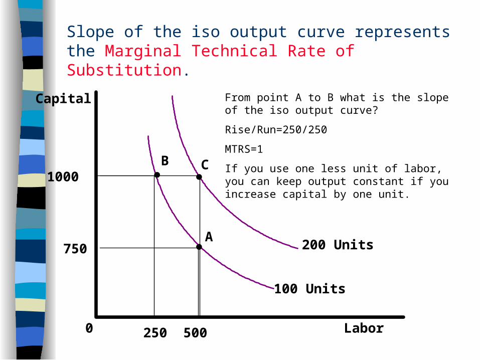
Slope of the iso output curve represents the Marginal Technical Rate of Substitution.
Labor
Capital
0 500
750
1000
250
100 Units
200 Units
From point A to B what is the slope of the iso output curve?
Rise/Run=250/250
MTRS=1
If you use one less unit of labor, you can keep output constant if you increase capital by one unit.
B
A
C

Efficient Production. Once the firm has chosen how much to produce, it will produce
that amount in the most efficient way. Efficient production can be described three alternative but
equivalent ways:– The firm is producing efficiently if the firm is producing at a
point where the iso-output and iso-cost curve is tangent.– The firm is producing efficiently if it is on the highest iso-
output curve that has at least one point in common with an iso cost curve.
– The firm is producing efficiently where the slope of the iso cost curve and the iso output curve are equal.
Examine the intuition behind each way of describing efficient production.

Efficient Production
Labor
Capital
0 500
750
1000
400
100 Units
A
At point A, the firm is producing efficiently because its’ iso-cost and iso-output curve are tangent.
At point A, what is total cost if capital costs $25 and labor costs $50?
$750*$25+$500*$50=$18,750+$25,000=$43,750
What is the average cost of production?
$43,750/100=$437.50
B
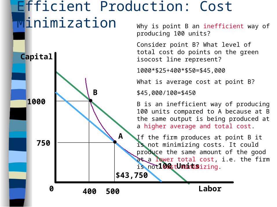
Efficient Production: Cost Minimization
Labor
Capital
0 500
750
1000
400
100 Units
A
Why is point B an inefficient way of producing 100 units?
Consider point B? What level of total cost do points on the green isocost line represent?
1000*$25+400*$50=$45,000
What is average cost at point B?
$45,000/100=$450
B is an inefficient way of producing 100 units compared to A because at B the same output is being produced at a higher average and total cost.
If the firm produces at point B it is not minimizing costs. It could produce the same amount of the good at a lower total cost, i.e. the firm is not cost minimizing.
$43,750
B

Efficient Production: Output Maximization
Labor
Capital
0 500
750
1000
400
100 Units
A
$43,750
B
C
150 Units
$45,000
Consider point C. How much capital is the firm using at point C?
($45,000-(500*50))/25=800 units
If the firm chooses to produce at point C, what is total cost?
1000*$25+400*$50=$45,000
What is average cost at point C?
$45,000/150=$300
If the firm changes how it produces the good from point B to C, it could produce more output for the same total cost.
Moving from B to C the firm is output maximizing—producing the most output given the amount being spent on inputs.
This would lower the average cost of production from $450 to $300.

Efficient Production: MTRS = Relative Price of inputs.
Labor
Capital
0 500
750
1000
400
100 Units
A
$43,750
B
At point D, how much capital is the firm using?
(43,750-(400*50))/25=950
Suppose the firm is producing at B. What is the MTRS and Relative Price of Labor.
MTRS=rise/run=250/100=2.5
Relative price of Labor=1000/500=2
At point B, MTRS>Relative Price of Labor.
If the firm used one 2.5 less units of capital it could keep production constant by using one more unit of labor.
If the firm used 2 units less capital it could buy one more unit of labor.
Therefore at point B, where the MTRS>Relative Price of Labor, the firm is not producing efficiently. It could reduce the amount of capital, use the money to buy more labor, keep output constant, and reduce total cost.
D

Efficient Production Revisited.
A firm is producing efficiently if it is:– Minimizing costs for the amount of the
good it is producing.– Maximizing output for the amount it is
expending on inputs.– Using a combination of inputs where
reducing the amount of one input, taking the saved money, and buying more of the other input, would not increase output.

Using iso-cost and iso-output curves to analyze two changes.
Suppose the price of an input changed.– How would this affect the production
decision of the firm? Suppose there was a change in
technology.– How would this affect the production
decision of the firm?

Analyzing a change in the price of inputs.
Labor
Capital
0 50
100
100 Units
A
$100,000
Consider a firm which has a total cost of $100,000, and produces 100 units of a good using 100 units of capital and 50 units of labor. Depict the situation on the graph below. If Capital costs $250 per unit, how much does labor cost?
Total Cost=Capital Cost +Labor Cost$100,000=100*250+50*Labor CostLabor Cost=($100,000-$25,000)/50=$1500
Suppose the price of Capital were to fall to $200 per unit. Draw the new iso-cost curve through A. How will it adjust it’s production process?
Once the price of capital has change, is the firm producing efficiently at A?

Analyzing a change in the price of inputs (2).
Labor
Capital
0 50
100
100 Units
A
$100,000
Before the drop in the price of capital, what is the total cost of production?
Total Cost =100*$250+50*$1500=$100,000
Average Total Cost=$100,000/100=$1,000
If the firm produces at A, what is the total and average total cost of production?
Total Cost =100*$200+50*$1500=$95,000
Average Total Cost=$95,000/100=$950
What has happened to ATC and TC after the drop in the price of capital?
TC has fallen from $100,000 to $95,000.
ATC has fallen from $1000 to $950.
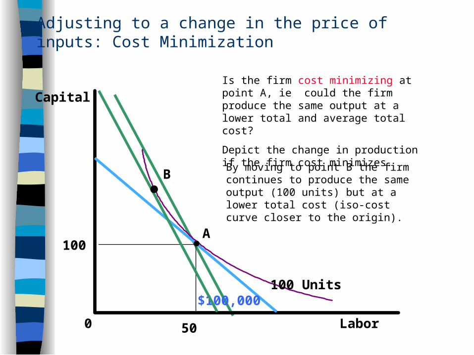
Adjusting to a change in the price of inputs: Cost Minimization
Labor
Capital
0 50
100
100 Units
A
$100,000
Is the firm cost minimizing at point A, ie could the firm produce the same output at a lower total and average total cost?
Depict the change in production if the firm cost minimizes.
BBy moving to point B the firm continues to produce the same output (100 units) but at a lower total cost (iso-cost curve closer to the origin).

Adjusting to a change in the price of inputs: Output Maximization
Labor
Capital
0 50
100
100 Units
A
$100,000
Is the firm output maximizing at point A, i.e. could the firm produce more output for the same total cost?
Depict the change in production if the firm output maximizes.
CBy moving to point C the firm keeps total cost constant (stays on the same iso-cost curve) but increase output (moves to a higher iso-output curve).
Explain using MTRS and relative price why the firm is not producing efficiently at A after the price of capital has changed.
The firm could reduce the amount of labor, take the money saved, spend it on capital and increase output.

Analyzing a change in technology.
Labor
Capital
0 50
100
100 Units
A
$100,000
Consider the same firm which has a total cost of $100,000, and produces 100 units of the good using 100 units of capital and 50 units of labor. Capital costs $250 per unit and labor costs $1500 per unit.
200 Units
Suppose an improvement in technology occurred which allowed the firm to produce twice as much output with the same labor and capital.
Depict such a change on the graph.

Analyzing a different change in technology.
Labor
Capital
0 50
100
100 Units
A
$100,000
Consider the same firm which has a total cost of $100,000, and produces 100 units of the good using 100 units of capital and 50 units of labor. Capital costs $250 per unit and labor costs $1500 per unit.
25
B
Suppose someone invented a machine which costs the same as the machines in use now but could produce the same output with half as much labor.
Draw the iso-output curve for 100 units of output.
Advanced question: Is the MTRS (the slope of the iso-output curve) at B greater or less than at A? Explain.
Variable and Fixed Costs Iso-cost and iso-output curves can be used to
analyze the difference between fixed and variable costs.
The short and long run.– The short run is period so short that the amount of
some inputs cannot be changed,i.e. some inputs are fixed.
– The long run is a period long enough that all inputs are changed i.e. all inputs become variable.
Consider how a firm adjusts production to vary input in the short and long run. – For examples, capital is the fixed input and labor is
the variable input.

Changing output in the short and long run.
Labor
Capital
0 50
100
100 Units
A
$100,000
Suppose the firm is considering a short run change in output, i.e. the amount of capital is fixed.
Depict the change in output if the firm increases output to 110 units in the short run.
110 UnitsB
75
Consider the same firm which has a total cost of $100,000, and produces 100 units of the good using 100 units of capital and 50 units of labor. Capital costs $250 per unit and labor costs $1500 per unit.

Changing output in the short and long run.
Labor
Capital
0 50
100
100 Units
A
$100,000
Suppose the firm is considering a long run change in output, i.e. the amount of capital and labor are variable.
Depict the change in output if the firm increases output to 110 units in the long run.
110 UnitsB
75
Consider the same firm which has a total cost of $100,000, and produces 100 units of the good using 100 units of capital and 50 units of labor. Capital costs $250 per unit and labor costs $1500 per unit.
C
55
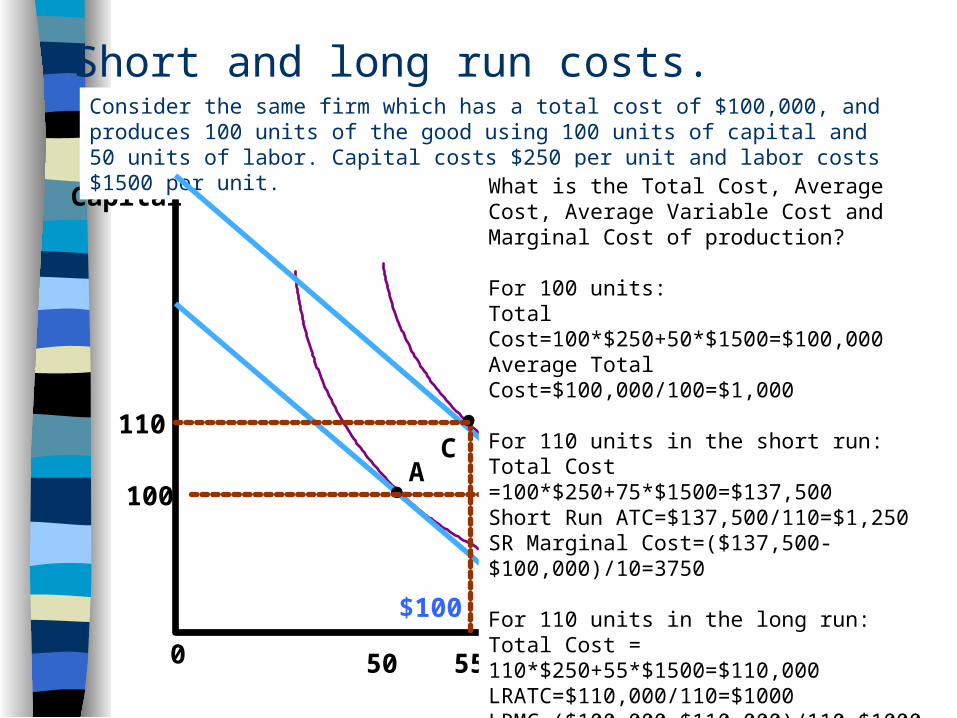
Short and long run costs.
Labor
Capital
0 50
100
100 Units
A
$100,000
110 UnitsB
75
Consider the same firm which has a total cost of $100,000, and produces 100 units of the good using 100 units of capital and 50 units of labor. Capital costs $250 per unit and labor costs $1500 per unit.
C
55
110
What is the Total Cost, Average Cost, Average Variable Cost and Marginal Cost of production?
For 100 units:Total Cost=100*$250+50*$1500=$100,000Average Total Cost=$100,000/100=$1,000
For 110 units in the short run:Total Cost =100*$250+75*$1500=$137,500Short Run ATC=$137,500/110=$1,250SR Marginal Cost=($137,500-$100,000)/10=3750
For 110 units in the long run:Total Cost = 110*$250+55*$1500=$110,000LRATC=$110,000/110=$1000LRMC=($100,000-$110,000)/110=$1000
Sample Exam Question: Can you explain, without using technical jargon, why
the MC is greater in the short run than in the long run?
Answer: – In the long run, the firm has the ability to vary all
inputs to the production process. – In the short run, the firm can only vary its’ variable
inputs. – The greater degree of flexibility in the long run
allows the firm to adjust better to changes in output.
– Therefore, its’ MC , the cost of producing more output, and ATC are generally lower in the long run than in the short run.
Cost Curves and the Output Decision of the Firm
To properly make the decision how much to produce (as opposed to the question of how to produce) the firm must measure the unit cost of production in four ways.– Average Short Run Total Cost– Average Long Run Total Cost– Average Variable Cost– Marginal Cost
Each of these measures of unit cost can be derived using iso-cost/iso-output analysis. – Be able to do this for exam.
A firm can use these measures of unit cost to decide how much to produce in a competitive market.
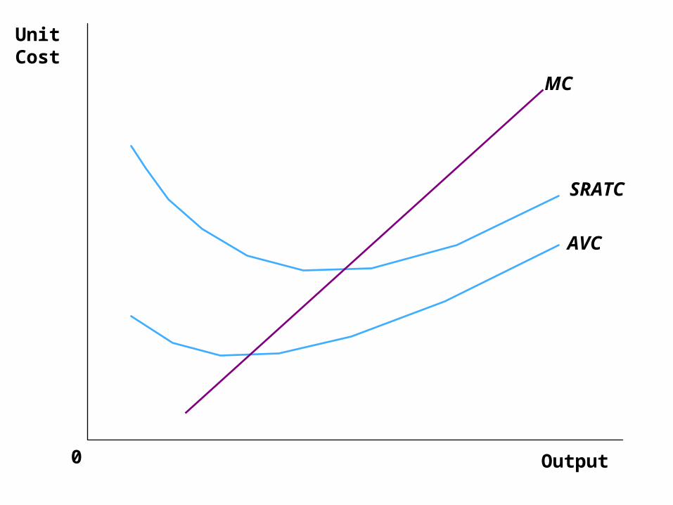
Output0
Unit Cost
MC
SRATC
AVC

The Meaning of Competition
A perfectly competitive market has the following characteristics:– There are many buyers and sellers in the market.– The goods offered by the various sellers are
largely the same-homogeneous good.– Firms can freely enter or exit the market.– The individual firm produces a small portion of
total market output.– The firm cannot have any influence over the price
it charges

The Meaning of Competition
The individual firm in a perfectly competitive market is a price taker.– It takes the price determined by the market
as the price that it will receive for its output.– When making decisions, the price taking
firm can assume that it can sell as much of the good as it wants at the market price.
Profit Maximization for the Competitive Firm
The goal of a competitive firm is to maximize profit. The firm in a competitive market can maximize profits
by applying the 3-part output rule of a price taking firm.– Shutdown Decision: Should if produce at all?– Short Run Output Decision: If the firm is going to
produce how much should it produce in the short run?
– Long Run Entry and Exit Decision: In the long run, should the firm stay in business?
Examine each of these three decision in detail.
The Firm’s Decision to Shut Down
The firm should shutdown in the short run, i.e. produce nothing if the price is below the minimum AVC of production.– If the price is below the min. AVC, the firm would lose less by
shutting down. • If the firm shutdown, it would lose only its’ fixed costs. • If it produced, it would lose its’ fixed costs and a portion of its’
variable costs. • Therefore, it would lose less in the short run by shutting down.
– If the price is between the min. AVC and the min. ATC, the firm should produce even though it loses money by doing so.
• The price it is getting is sufficient to cover its variable costs and a portion of its’ fixed costs.
• Therefore the firm will lose less by producing than it would be shutting down.
– If the price is above the min. ATC, the the firm can produce at a profit.
• The price it is getting is sufficient to cover all of its’ costs.

The Firm’s Decision to Shut Down
Quantity
MC
ATC
AVC
0
CostsIf P > min ATC, The firm is covering its’ fixed and variable costs, is Earning a profit and should continueProducing.
If min AVC<P <min ATC, The firm should keep producing in the short run. It is covering its’ variablecosts and a portion of its’ fixed costs. Therefore,It loses less by producing than shutting down.

The Firm’s Decision to Shut Down
Quantity
MC
ATC
AVC
0
CostsIf P < min AVC then the firm should shut down.
If it produces, the price it is getting will not coverEven its’ variable costs.
If it produces the firm will lose its fixed costs plus a portion of its variable costs.
Therefore, it loses less by shutting down.
The Firm’s Decision to Shut Down The portion of the marginal-cost curve
that lies above average variable cost is the competitive firm’s short-run supply curve.

The Firm’s Decision to Shut Down
Quantity
MC
ATC
AVC
0
Costs
Firm’s short-runsupply curve

Profit Maximization for the Competitive Firm If the firm has made the shutdown decision and
decided not to shutdown, the next decision the firm must make is how much to produce.
The firm can determine the profit maximizing (or loss minimizing) level of output by setting P=MC.
An alternative way of determining the profit maximizing level of output is to use the following rule:– If P>MC increase output.– If P<MC decrease output.– If P=MC leave output unchanged.

Profit Maximization for the Competitive Firm
Quantity0
Costsand
RevenueMC
ATC
AVC P P = AR = MR

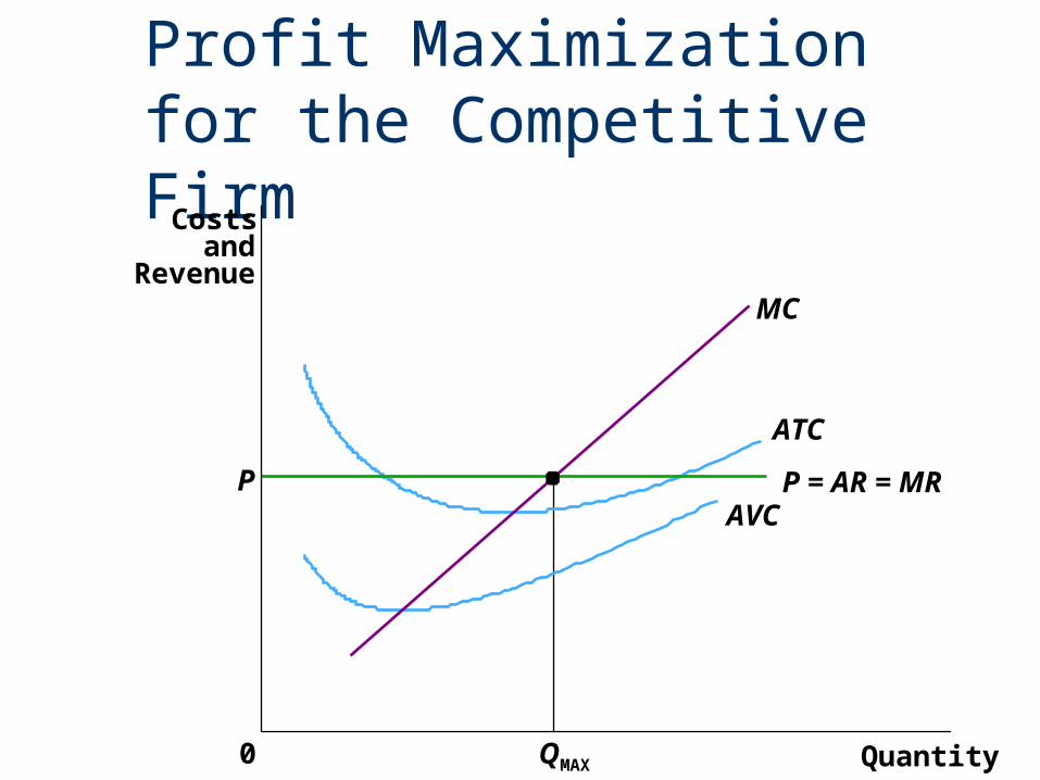
Profit Maximization for the Competitive Firm
Quantity0
Costsand
RevenueMC
ATC
AVC
QMAX
P = AR = MR
The firm maximizesprofit by producingthe quantity at whichmarginal cost equalsmarginal revenue.
P

Profit Maximization for the Competitive Firm A competitive firm will adjust its
production level until quantity reaches QMAX where profit is maximized.
Profit Maximization for the Competitive Firm
Quantity0
Costsand
RevenueMC
ATC
AVC
QMAX
P = AR = MR P

Profit Maximization for the Competitive Firm
Quantity0
Costsand
RevenueMC
ATC
AVC
MC1
Q1 QMAX
P = MR1 P = AR = MR
If the firm is producing Q1 when the P=MR1, the firm is not maximizing profit.
What could the firm do to increase profits? Why?
If it increased output by one unit, the extra cost the firm would incur (its MC) would be less than the extra revenue it would receive from selling that one extra unit produced (the price or marginal revenue).
Therefore, the firm would increase its’ profit or reduce its’ loss by expanding output.

Profit Maximization for the Competitive Firm
Quantity0
Costsand
RevenueMC
ATC
AVC
MC1
Q1 QMAX
P = MR1 P = AR = MR
P > MC,
increase Q

Profit Maximization for the Competitive Firm
Quantity0
Costsand
RevenueMC
ATC
AVC
MC2
Q2QMAX
P = MR2 P = AR = MR
If the firm is producing Q2 when the P=MR1, the firm is not maximizing profit.
What could the firm do to increase profits? Why?
If it decreased output by one unit, the extra cost the firm would save (its MC) would be more than the extra revenue it would forego from selling one fewer unit (the price).
Therefore, the firm would increase its’ profit or reduce its’ loss by reducing output.

Profit Maximization for the Competitive Firm
Quantity0
Costsand
RevenueMC
ATC
AVC
MC2
Q2QMAX
P = MR2 P = AR = MR
P < MC,
decrease Q
The Long-Run Decision to Exit an Industry In the long-run, the firm exits if the
revenue it would get from producing is less than its total cost.– Exit if P<min ATC.
New firms will enter the industry if such an action would be profitable.– Enter if P >min ATC
The Competitive Firm’s Long-Run Supply Curve
Quantity
MC
ATC
AVC
0
Costs

The Competitive Firm’s Long-Run Supply Curve
Firm enters if P > ATC
Quantity
MC
ATC
AVC
0
Costs

The Competitive Firm’s Long-Run Supply Curve
Firm enters if P > ATC
Firm exitsif P < ATC
Quantity
MC
ATC
AVC
0
Costs

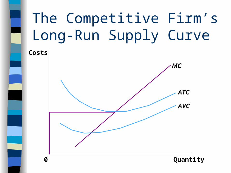
The Competitive Firm’s Long-Run Supply Curve The competitive firm’s long-run supply
curve is the portion of its marginal-cost curve that lies above average total cost.

The Competitive Firm’s Long-Run Supply Curve
Quantity
MC
ATC
AVC
0
Costs
Firm’s long-runsupply curve
The competitive firm’s long-run supply curve is the portion of its marginal-cost curve that lies above average total cost.

The Firm’s Short-Run and Long-Run Supply Curves Short-Run Supply Curve The portion of its marginal cost curve that
lies above average variable cost. Long-Run Supply Curve The marginal cost curve above the
minimum point of its average total cost curve.

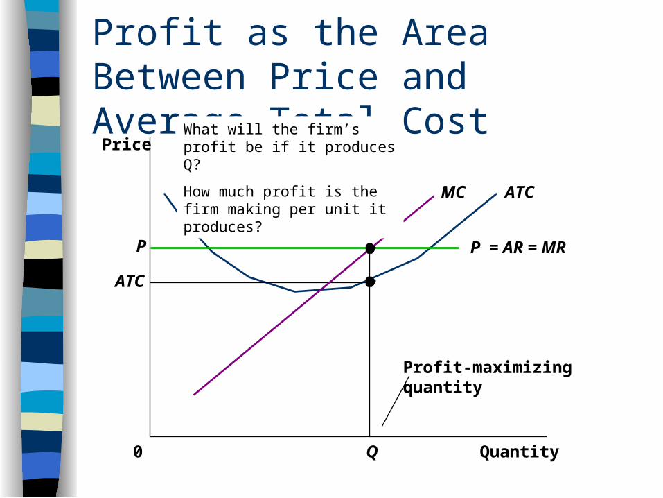
Profit as the Area Between Price and Average Total Cost
Quantity0
Price
P = AR = MR
ATCMC
P
At this price, how much will the firm produce?
Profit as the Area Between Price and Average Total Cost
Quantity0
Price
ATCMC
P
ATC
Q
Profit-maximizingquantity
P = AR = MR
What will the firm’s profit be if it produces Q?
How much profit is the firm making per unit it produces?
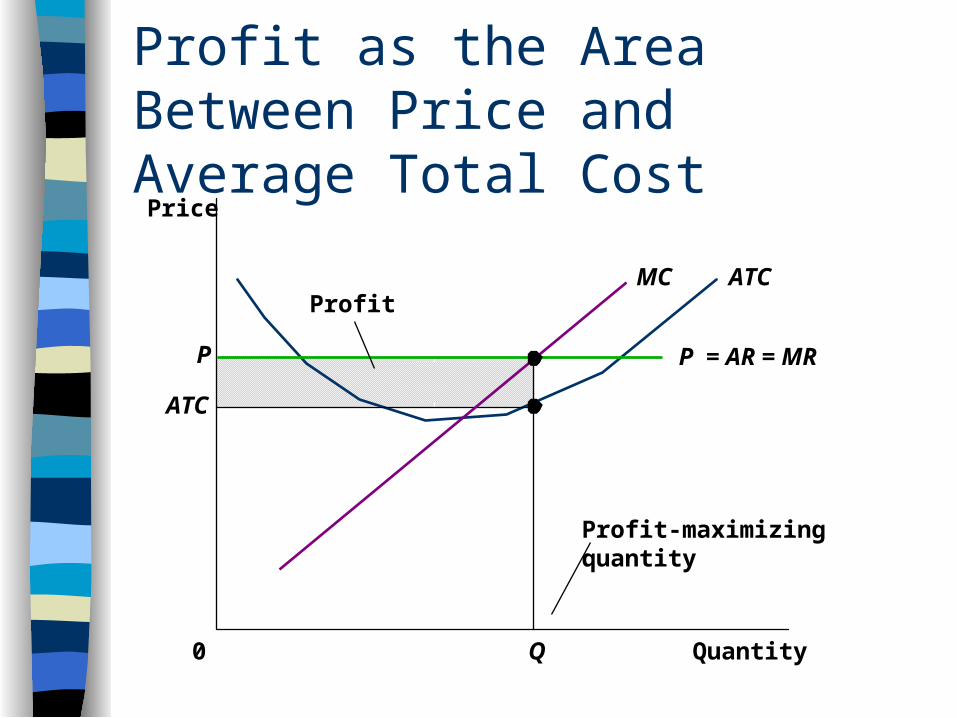
Profit as the Area Between Price and Average Total Cost
Quantity0
Price
ProfitATCMC
P
ATC
Q
Profit-maximizingquantity
P = AR = MR

Loss as the Area Between Price and Average Total Cost
Quantity0
Price
ATCMC
P P = AR = MR
AVC
If the price is P, will the firm shutdown?
If it produces, how much should it produce?
Will it be earning a profit?
What will its’ loss be?
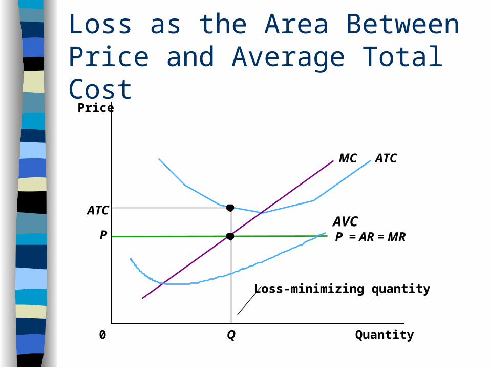
Loss as the Area Between Price and Average Total Cost
Quantity0
Price
ATC
ATCMC
Q
Loss-minimizing quantity
P P = AR = MRAVC
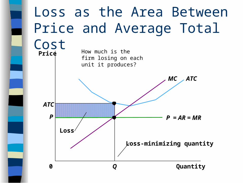
Loss as the Area Between Price and Average Total Cost
Quantity0
Price
ATC
Loss
ATCMC
Q
Loss-minimizing quantity
P P = AR = MR
How much is the firm losing on each unit it produces?
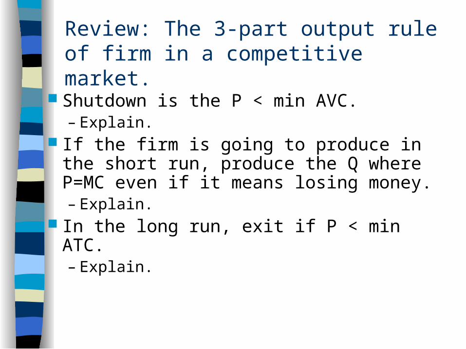
Review: The 3-part output rule of firm in a competitive market.
Shutdown is the P < min AVC.– Explain.
If the firm is going to produce in the short run, produce the Q where P=MC even if it means losing money.– Explain.
In the long run, exit if P < min ATC. – Explain.
Market Supply in a Competitive Market
Market supply equals the sum of the quantities supplied by the individual firms in the market.
Market Supply with a Fixed Number of Firms (Short Run Supply Curve).– For any given price, each firm supplies a quantity of output so that
price equals its marginal cost. – The market supply curve reflects the individual firms’ marginal cost
curves. Market Supply with Entry and Exit (Long Run Supply Curve).
– Firms will enter or exit the market until profit is driven to zero.– In the long-run, price equals the minimum of average total cost.– The long-run market supply curve is horizontal at this price
(constant cost industry).

The Supply Curve in a Competitive Market(a) Firm’s Zero-Profit Condition
Quantity(firm)
0
Price
P =minimum
ATC
(b) Market Supply
Quantity(market)
Price
0
Long RunSupply
MC
ATC

Initial Condition
MarketFirm
Quantity(firm)
0
Price
MC ATC
P1
Quantity(market)
Price
0
D1
P1
Q1
A
S1
Long-runsupply

Short-Run Response to an increase in Demand
MarketFirm
Quantity(firm)
0
Price
P1
Quantity(market)
Price
0
D1
D2
P1
Q1
A
S1
Long-runsupply
MC ATC
P1
B
The increase in demand (D1 to D2) causes the price in to increase.
At current output levels (Q1) the existing firms are producing where P >MC.
Therefore, they can increase profits by increasing output.
The increase in output by existing firms causes a movement along the short run supply curve (S1) from A to B.
Short-Run Response to an increase in Demand
MarketFirm
Quantity(firm)
0
Price
MC ATC
P1
P2
Quantity(market)
Price
0
D1
D2
P1
Q1 Q2
P2 A
B S1
Long-runsupply
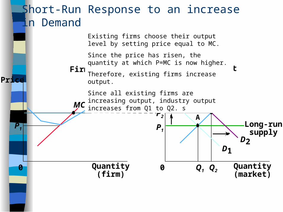
Existing firms choose their output level by setting price equal to MC.
Since the price has risen, the quantity at which P=MC is now higher.
Therefore, existing firms increase output.
Since all existing firms are increasing output, industry output increases from Q1 to Q2. s

Short-Run Response to an increase in Demand
MarketFirm
Quantity(firm)
0
Price
MC ATCProfit
P1
P2
Quantity(market)
Price
0
D1
D2
P1
Q1 Q2
P2 A
B S1
Long-runsupply

Increase in Demand in the Long Run Over time, the short-run supply curve shifts
as profits encourage new firms to enter the market.
Price falls as new firms enter the market In the new long-run equilibrium profits return
to zero and price returns to minimum average total cost.
The market has more firms to satisfy the greater demand.

Long-Run Response
MarketFirm
Quantity(firm)
0
Price
MC ATCProfit
P1
P2
Quantity(market)
Price
0
D1
D2
P1
Q1 Q2
P2 A
B S1
Long-runsupply
At price P2, existing firms are earning a profit.
Entrepreneurs see the profit earned by existing firms and open new firms (enter the industry).
Long-Run Response
MarketFirm
Quantity(firm)
0
Price
MC ATCProfit
P1
P2
Quantity(market)
Price
0
P1
Q1 Q2
P2 A
B
Long-runsupply
S2
D1
D2
S1
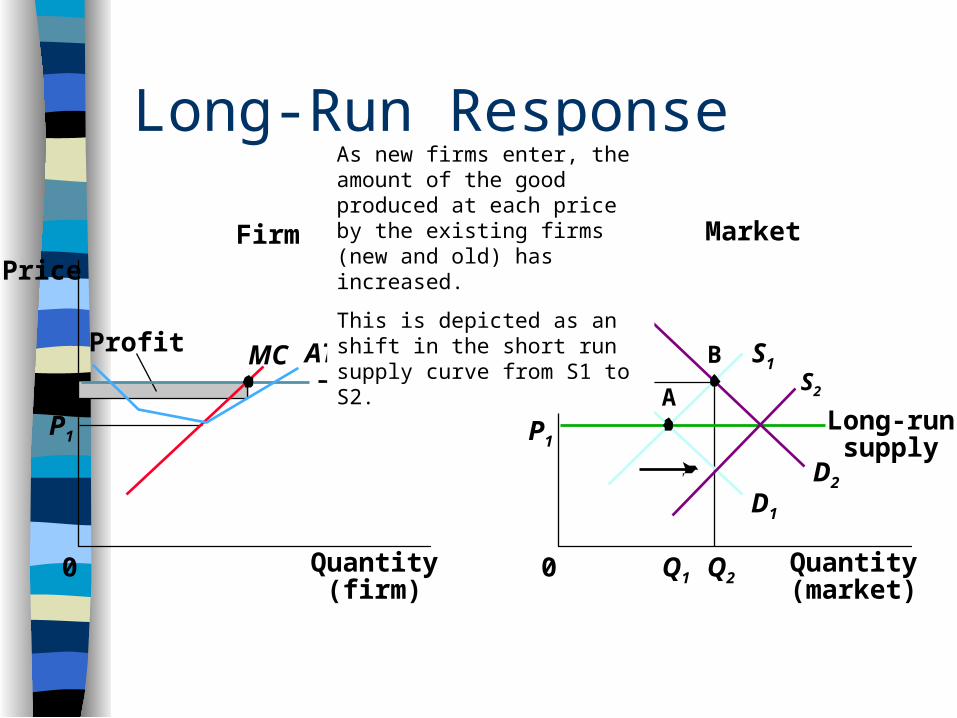
As new firms enter, the amount of the good produced at each price by the existing firms (new and old) has increased.
This is depicted as an shift in the short run supply curve from S1 to S2.
Long-Run Response
MarketFirm
Quantity(firm)
0
Price
MC ATC
P1
Quantity(market)
Price
0
D1
D2
P1
Q1 Q2
P2 A
B S1
Long-runsupply
S2
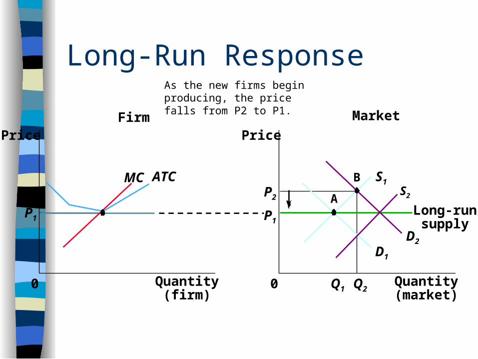
As the new firms begin producing, the price falls from P2 to P1.

Increase in Demand in the Short and Long Run
MarketFirm
Quantity(firm)
0
Price
MC ATC
P1
Quantity(market)
Price
0
D2
P1
Q1
D1
Q2
A
B S1
Long-runsupply
S2
Q3
C
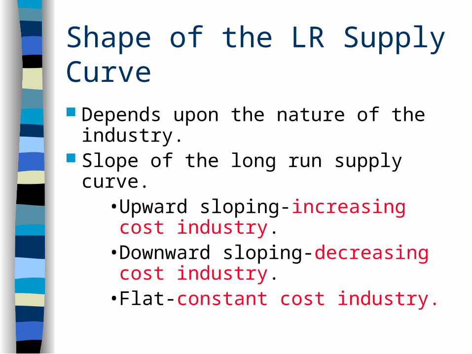
Shape of the LR Supply Curve
Depends upon the nature of the industry.
Slope of the long run supply curve.• Upward sloping-increasing cost
industry.• Downward sloping-decreasing cost
industry.• Flat-constant cost industry.

Market for Fatburgers. What is takes to own a Fatburger.
– Net Worth of $250,000 with $150,000 in liquid assets.– $30,000 franchise fee.– $370,000-$730,000 startup costs.– 25% of startup costs funded from personal resources.– Pay 5% of net sales.
Example of business in a box. Invest $500,000 and earn $200,000 in first year profits.

Long Run Supply Curve in Fatburger Market.

Basics of Oil Exploration
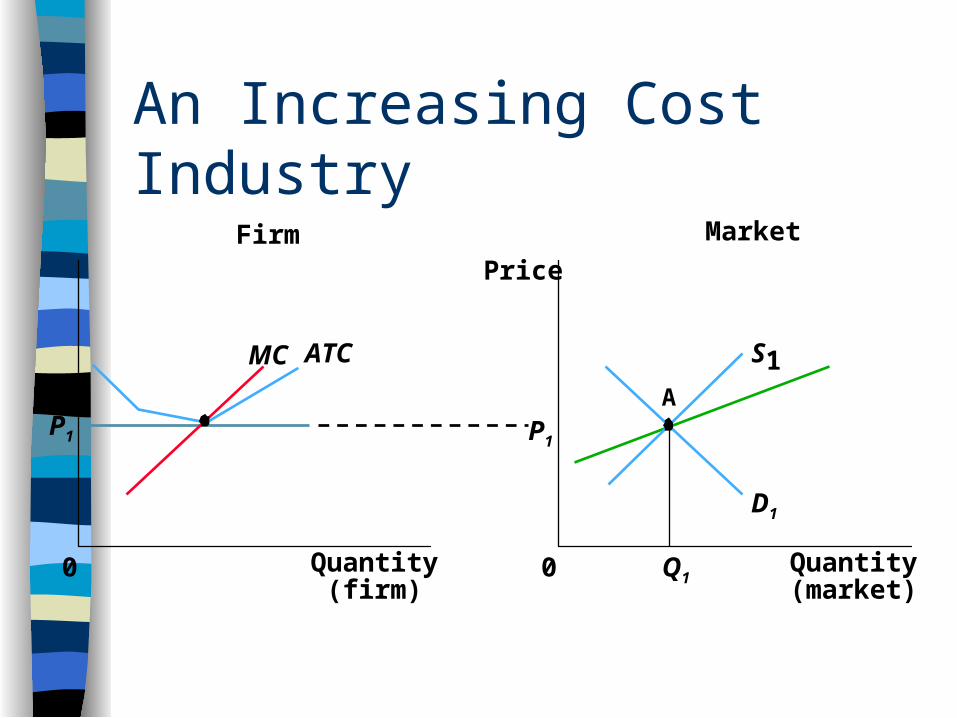
An Increasing Cost Industry
MarketFirm
Quantity(firm)
0
MC ATC
P1
Quantity(market)
Price
0
D1
P1
Q1
A
S1

Shape of the LR Supply Curve
The shape of the long run supply curve is determined by the min ATC of potential entrants.– If potential entrants have higher costs than
existing firms, the LR supply curve will be upward sloping (oil industry example).
– If potential entrants have the same costs as existing firms, the LR supply curve will be flat (business in a box example).

Constant Cost and Increasing Cost Industries. A constant cost industry is an industry
where potential entrants face the same unit costs as existing firms. – Example: Business in a box.
An increasing cost industry is an industry where potential entrants face higher unit costs than existing firms. – Example: Oil Industry

Administrative Details
Homework due Monday October 23.– Production and Cost Homework.
• Porsche homework.
Second Exam on Friday, November 3rd.– Chapters 5, 6, and 7 in Landsburg.

This graph shows changes in the market price and industry output of a good over time. Assume that by D all short and long run adjustments have been made. 1. What could cause the market price and output to change in the manner depicted below? Depict such a change on your graph. (hint: more than one thing may happen).2. Label points A, B, C and D on both graphs.Provide a brief narrative of the short and long run changes among firms. 3. Draw the long run industry supply curve. Is the industry an increasing cost or decreasing cost industry? Explain.

Answer A
MarketFirm
Quantity(firm)
0
Price
P1
Quantity(market)
Price
0
D1D 2
P1
Q1
S1
Long-runsupply
MC ATC
P1
A
P2
Demand shifts to the left, the market price falls, the existing firms reduce output by setting output where the new price, P2, equals MC. The existing firms are losing money but keep producing in the short run as long as P > min AVC.

Answer B
MarketFirm
Quantity(firm)
0
Price
P1
Quantity(market)
Price
0
D1D
2
P1
Q1
A
S1MC ATC
P1
P2
Because the existing firms are losing money by selling at a price P2, some firms exit the market. As firms exit the market, the short run supply curve shifts to the left from S1 to S2. Because there are fewer firms, less output is produced at every price and the price rises. At point B, the long run adjustment in the the number of firms has begun but has not been completed.
S2
B
S3
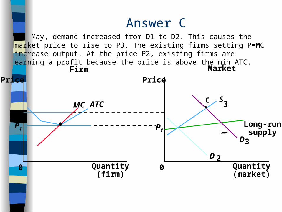
Answer C
MarketFirm
Quantity(firm)
0
Price
P1
Quantity(market)
Price
0
D 2
P1
D3
S3
Long-runsupply
MC ATC
P1
C
P3
In May, demand increased from D1 to D2. This causes the market price to rise to P3. The existing firms setting P=MC increase output. At the price P2, existing firms are earning a profit because the price is above the min ATC.

Answer DBecause existing firms are earning a profit, new firms will enter the industry. As news firms enter, the short run supply curve shifts to the right. At any price more is produced because there are more firms in the industry. The extra production lowers price.
MarketFirm
Quantity(firm)
0
Price
P1
Quantity(market)
Price
0
D 2
D3
P1
S3
Long-runsupply
MC ATC
P1
C
P3S4
D

Production with One Variable Input
Take an alternative look at the production process—short and long run output decisions, fixed and variable inputs, etc.
Look at the problem of efficient production from the point of view of a firm which only has control over one input. The other inputs to the production process are fixed.
Consider an example: – A hog farm where the number of pigs is the fixed input and
the amount of corn the pigs are fed is the variable input. – Assume that pork can be sold for $.75 and corn costs $10
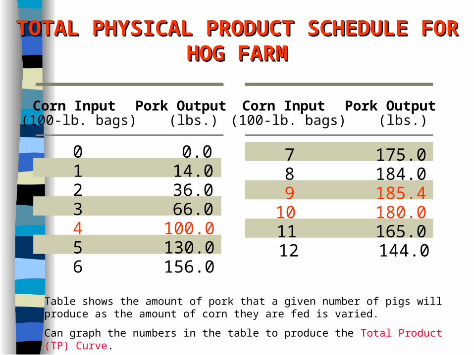
per bag. Total physical product = the amount of output that can be
produced as one input changes, with all other inputs held constant.
TOTAL PHYSICAL PRODUCT SCHEDULE TOTAL PHYSICAL PRODUCT SCHEDULE FOR HOG FARMFOR HOG FARM
7 8 9
10 11 12
0 1 2 3 4 5 6
0.0 14.0 36.0 66.0
100.0 130.0 156.0
175.0 184.0 185.4 180.0 165.0 144.0
Corn Input (100-lb. bags)
Pork Output (lbs.)
Corn Input (100-lb. bags)
Pork Output (lbs.)
Table shows the amount of pork that a given number of pigs will produce as the amount of corn they are fed is varied.
Can graph the numbers in the table to produce the Total Product (TP) Curve.

0
20
40
60
80
100
120
140
160
180
200
2 4 6 8 10 12
Quantity of Corn (bags per week)
Tota
l Ou
tpu
t (p
ou
nd
s o
f p
ork
per
wee
k)
9
AB
C
D
E
F
G
HI J
K
L
M
TPP
TOTAL TOTAL PHYSICALPHYSICALPRODUCTPRODUCTWITHWITHDIFFERENTDIFFERENTQUANTITIESQUANTITIESOF CORNOF CORNFORFORPIGPIGFARMFARM
Production with One Variable Input
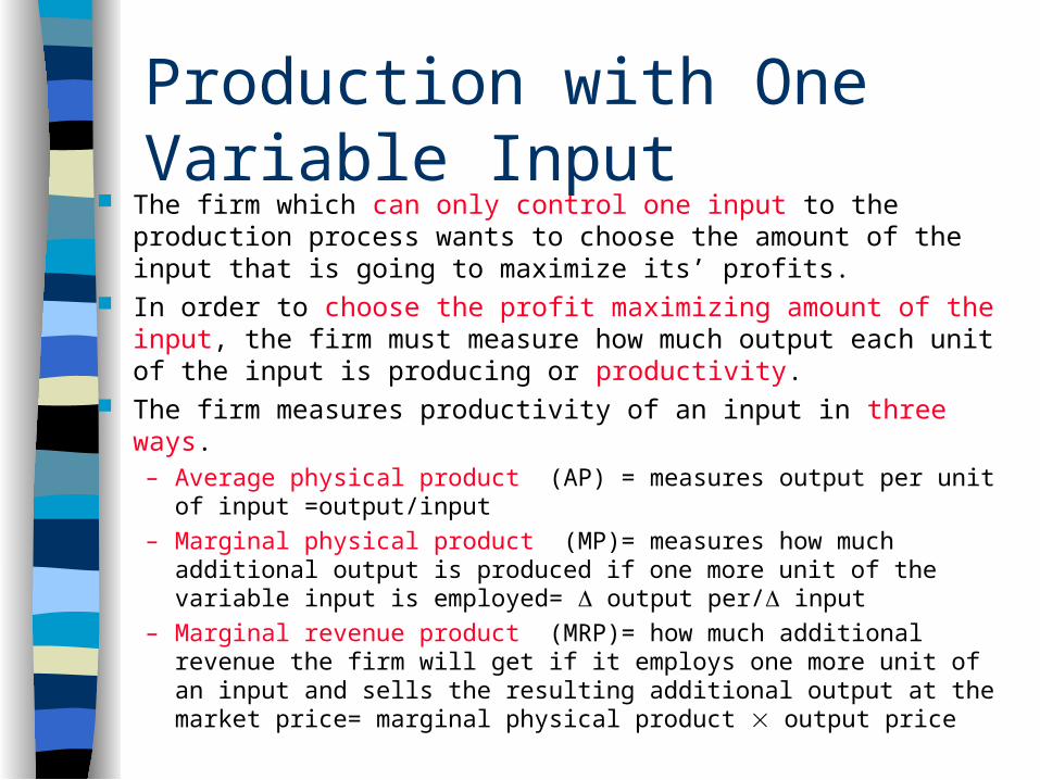
The firm which can only control one input to the production process wants to choose the amount of the input that is going to maximize its’ profits.
In order to choose the profit maximizing amount of the input, the firm must measure how much output each unit of the input is producing or productivity.
The firm measures productivity of an input in three ways. – Average physical product (AP) = measures output per unit of input
=output/input
– Marginal physical product (MP)= measures how much additional output is produced if one more unit of the variable input is employed= output per/ input
– Marginal revenue product (MRP)= how much additional revenue the firm will get if it employs one more unit of an input and sells the resulting additional output at the market price= marginal physical product output price
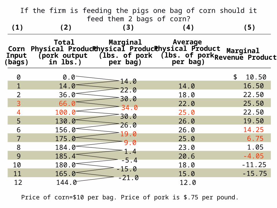
Marginal Revenue Product
(5)
0 1 2 3 4 5 6 7 8 9
10 11 12
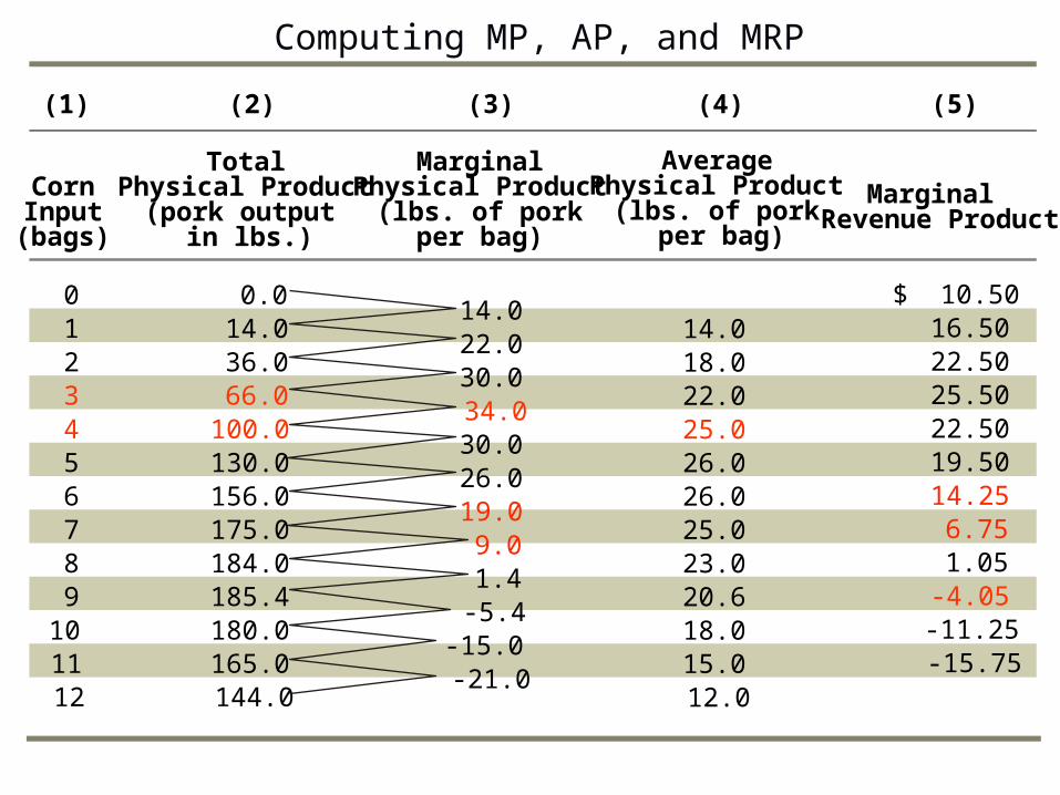
Corn Input
(bags)
(1)
Total Physical Product
(pork output in lbs.)
0.0 14.0 36.0 66.0
100.0 130.0 156.0 175.0 184.0 185.4 180.0 165.0 144.0
(2)
Average Physical Product
(lbs. of pork per bag)
14.0 18.0 22.0 25.0 26.0 26.0 25.0 23.0 20.6 18.0 15.0 12.0
(4)
Marginal Physical Product
(lbs. of pork per bag)
14.0 22.0 30.0 34.0 30.0 26.0 19.0 9.0 1.4
-5.4 -15.0 -21.0
(3)
$ 10.50 16.50 22.50 25.50 22.50 19.50 14.25 6.75 1.05
-4.05 -11.25 -15.75
Computing MP, AP, and MRP
0
20
40
60
80
100
120
140
160
180
200
2 4 6 8 10 12
Quantity of Corn (bags per week)
Tota
l Ou
tpu
t (p
ou
nd
s o
f p
ork
per
wee
k)
9
AB
C
D
E
F
G
HI J
K
L
M
TPP
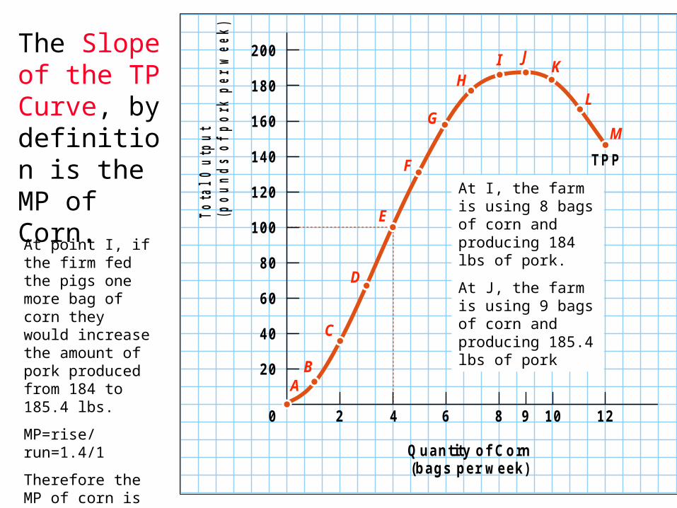
The Slope of the TP Curve, by definition is the MP of Corn.
At point I, if the firm fed the pigs one more bag of corn they would increase the amount of pork produced from 184 to 185.4 lbs.
MP=rise/run=1.4/1
Therefore the MP of corn is 1.4 lbs of pork.
At I, the farm is using 8 bags of corn and producing 184 lbs of pork.
At J, the farm is using 9 bags of corn and producing 185.4 lbs of pork

-240
MP
P
(po
un
ds
of
po
rk p
er
we
ek)
-20-16-12
-8-4048
12162024283236
2 4 6 8 10 12
Quantity of Corn Input (bags per week)
Increasing marginal returns
Diminishing marginal returns
Negative marginal returns
MPP
9
MARGINAL PHYSICAL PRODUCT MARGINAL PHYSICAL PRODUCT FOR PIG FARMFOR PIG FARM

Relationship between TP, AP, MP curves
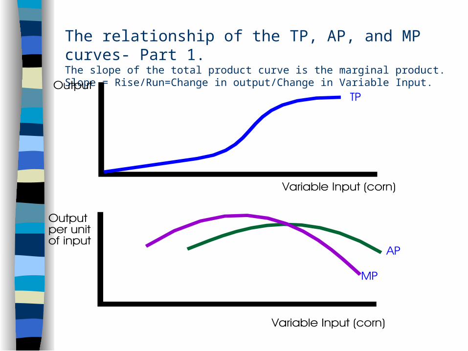
The relationship of the TP, AP, and MP curves- Part 1.The slope of the total product curve is the marginal product.Slope = Rise/Run=Change in output/Change in Variable Input.

The relationship of the TP, AP, and MP curves- Part 2.The point of inflection on the TP curve is the point of maximum MP.
To the left of the inflection point, the slope of the TP curve is increasing as the amount of the variable input is increased.
Since the slope of the TP curve is MP and the slope is increasing, MP must be increasing.
On the lower graph, to the left of the inflection point, the MP is increasing.

The relationship of the TP, AP, and MP curves- Part 3.When MP > AP, AP must be increasing as output increases.
When MP<AP, AP must be decreasing as output increases.

The Relationship Between Marginal and AverageAn Example.
When marginal is greater than average, average in increasing.
Consider the average height of a family.
Mommy-5 ft. tall
Daddy 6 ft. tall
Junior 7 ft. tall
Sister 6’1” ft. tall
What happens to the average height of the family as Sister is added?
Average height increases because before Sister arrived the average height of the family is 6 ft. and Sister is 6’1”.
Therefore the height of the marginal person is greater than the height of the people already in the group so average must be increasing.

The Relationship Between Marginal and Average-Second Example.
•What does GPA stand for?
•Grade Point Average
•What does AP stand for?
•Academic Probation
•If a student has a 1.8 GPA at CSUN what will happen to them.
•One semester to remedy.
•Academic Contracts, allocation of scarce class seats, and time to graduation.
•Expulsion or Concurrent Enrollment.
•If a student has an average GPA of 1.8 in all the class he has already taken, what grade point must he earn in the next class he takes if he is to increase his GPA?
•Answer: greater than 1.8, i.e. the marginal grade must be greater than the average grade in order for the average to rise.

An Alternative Way of Thinking About the Short Run Output Decision.
Marginal revenue product = marginal physical product output price
The amount of an input is optimal when marginal revenue product = price of the input.
The the MRP of an input is greater than the price of the input use more of the input.
Marginal Revenue Product
(5)
0 1 2 3 4 5 6 7 8 9
10 11 12
Corn Input
(bags)
(1)
Total Physical Product
(pork output in lbs.)
0.0 14.0 36.0 66.0
100.0 130.0 156.0 175.0 184.0 185.4 180.0 165.0 144.0
(2)
Average Physical Product
(lbs. of pork per bag)
14.0 18.0 22.0 25.0 26.0 26.0 25.0 23.0 20.6 18.0 15.0 12.0
(4)
Marginal Physical Product
(lbs. of pork per bag)
14.0 22.0 30.0 34.0 30.0 26.0 19.0 9.0 1.4
-5.4 -15.0 -21.0
(3)
$ 10.50 16.50 22.50 25.50 22.50 19.50 14.25 6.75 1.05
-4.05 -11.25 -15.75
If the firm is feeding the pigs one bag of corn should it feed them 2 bags of corn?
Price of corn=$10 per bag. Price of pork is $.75 per pound.

Computing Unit Cost- Fill in AVC, ATC, and MC
Variable Input Ouput MP AP
Fixed Cost
Variable Cost Total Cost AVC ATC MC
0 0 $201 14 14 14 $202 36 22 18 $203 66 30 22 $204 100 34 25 $205 130 30 26 $206 156 26 26 $207 175 19 25 $208 184 9 23 $209 185.4 1.4 20.6 $20
Price of the Variable Input=$10, Fixed Cost =$20

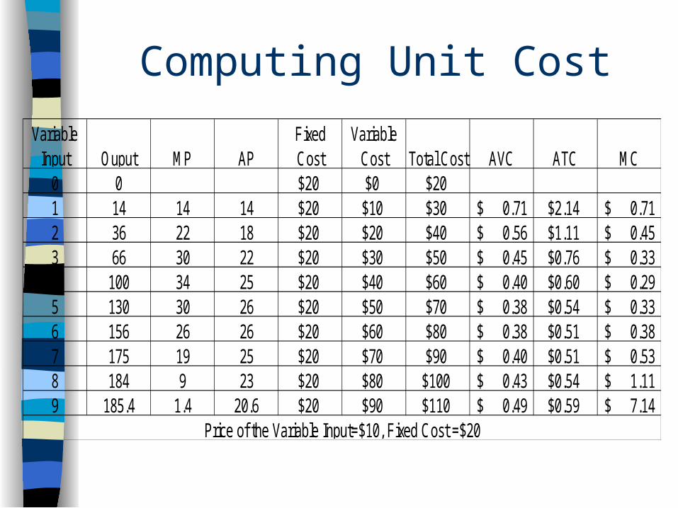
Computing Unit Cost
Variable Input Ouput MP AP
Fixed Cost
Variable Cost Total Cost AVC ATC MC
0 0 $20 $0 $201 14 14 14 $20 $10 $30 0.71$ $2.14 0.71$ 2 36 22 18 $20 $20 $403 66 30 22 $20 $30 $504 100 34 25 $20 $40 $605 130 30 26 $20 $50 $706 156 26 26 $20 $60 $807 175 19 25 $20 $70 $908 184 9 23 $20 $80 $1009 185.4 1.4 20.6 $20 $90 $110
Price of the Variable Input=$10, Fixed Cost =$20
Computing Unit Cost
Variable Input Ouput MP AP
Fixed Cost
Variable Cost Total Cost AVC ATC MC
0 0 $20 $0 $201 14 14 14 $20 $10 $30 0.71$ $2.14 0.71$ 2 36 22 18 $20 $20 $40 0.56$ $1.11 0.45$ 3 66 30 22 $20 $30 $50 0.45$ $0.76 0.33$ 4 100 34 25 $20 $40 $60 0.40$ $0.60 0.29$ 5 130 30 26 $20 $50 $70 0.38$ $0.54 0.33$ 6 156 26 26 $20 $60 $80 0.38$ $0.51 0.38$ 7 175 19 25 $20 $70 $90 0.40$ $0.51 0.53$ 8 184 9 23 $20 $80 $100 0.43$ $0.54 1.11$ 9 185.4 1.4 20.6 $20 $90 $110 0.49$ $0.59 7.14$
Price of the Variable Input=$10, Fixed Cost =$20
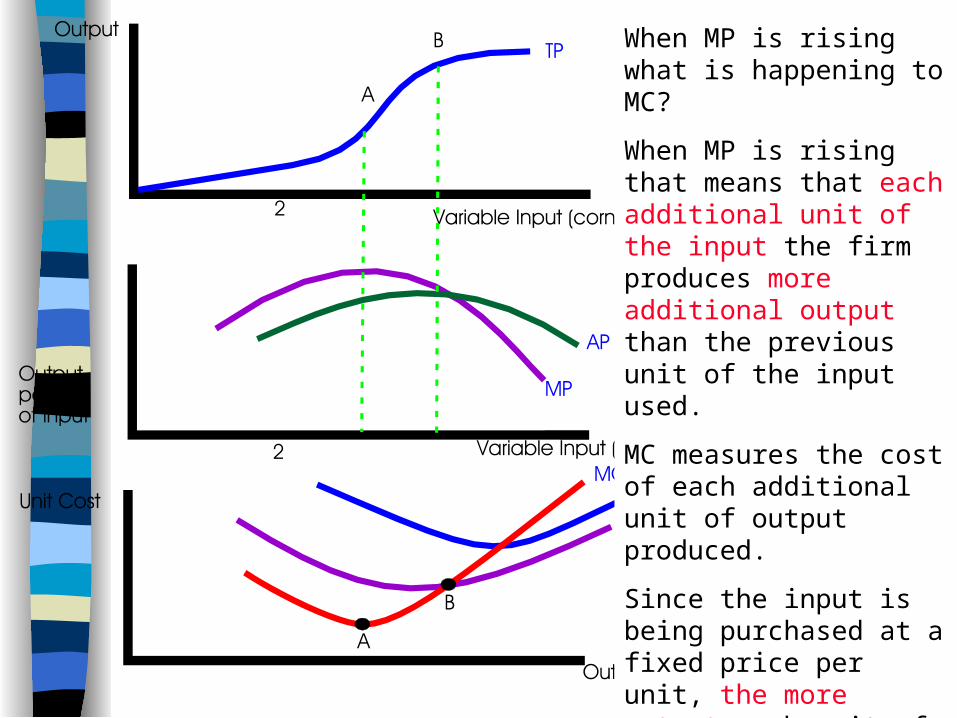
When MP is rising what is happening to MC?
When MP is rising that means that each additional unit of the input the firm produces more additional output than the previous unit of the input used.
MC measures the cost of each additional unit of output produced.
Since the input is being purchased at a fixed price per unit, the more output each unit of the input is producing the cheaper each unit of output.
Therefore, when MP is rising, MC must be falling.

When MP is at a maximum, what is happening to MC?
If MC is rising to the left of point A, MC must be falling to the left of point A.
IF MC is falling to the right of point A, MC must be rising to the right of point A.
Therefore, MC must be at a minimum at point A.

When AP is rising, what is happening to AVC?
AP measures the average amount of a good that is being produced per unit of the variable input used.
When AP is rising, the amount of the good being produced for each unit of the variable input being used is rising.
Since each unit of the variable input is being purchased at a constant price, the more that each unit of input produces the lower the average variable cost.
When AP is at a maximum, what is happening to AVC?

When AP is at a maximum, what is happening to AVC?
To the left of B, AP is rising as output increases.
Therefore AVC is falling to the left of B.
To the right of B, AP is falling as output increases.
Therefore AVC is rising to the right of B.
If AVC is falling to the left of B and rising to the right of B, then AVC must be at a minimum at point B.

A Change in Demand-The Complete Analysis
Suppose the market starts off in long run equilibrium.– The existing firms are earning a normal rate of
return at the market price.– The situation is depicted in the following graph. – The Industry consists of 10 firms producing a
homogeneous good.• Suppose capital costs $20 per unit.
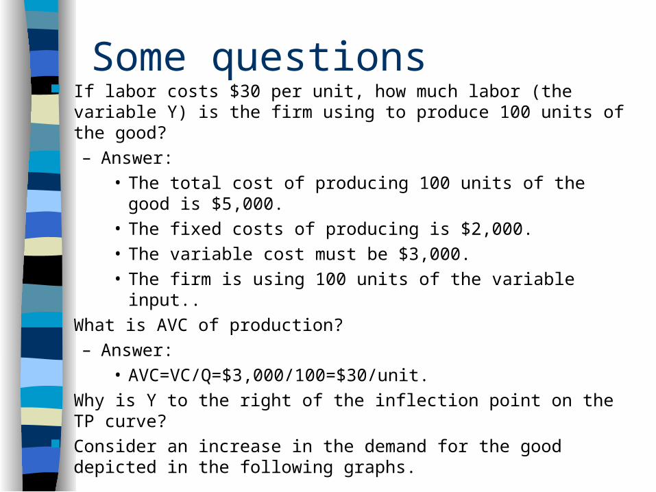
Some questions If labor costs $30 per unit, how much labor (the variable Y) is the firm
using to produce 100 units of the good?– Answer:
• The total cost of producing 100 units of the good is $5,000.• The fixed costs of producing is $2,000.• The variable cost must be $3,000.• The firm is using 100 units of the variable input..
What is AVC of production?– Answer:
• AVC=VC/Q=$3,000/100=$30/unit. Why is Y to the right of the inflection point on the TP curve? Consider an increase in the demand for the good depicted in the
following graphs.
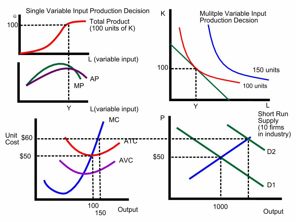
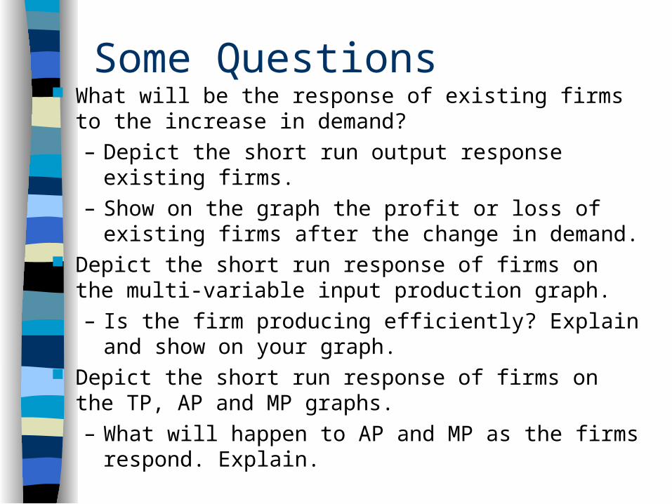
Some Questions What will be the response of existing firms to the
increase in demand?– Depict the short run output response existing firms.– Show on the graph the profit or loss of existing firms
after the change in demand. Depict the short run response of firms on the multi-
variable input production graph.– Is the firm producing efficiently? Explain and show on
your graph. Depict the short run response of firms on the TP, AP and
MP graphs.– What will happen to AP and MP as the firms respond.
Explain.

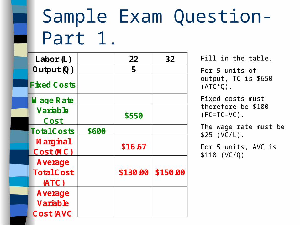
Sample Exam Question-Part 1.
Fill in the table.
For 5 units of output, TC is $650 (ATC*Q).
Fixed costs must therefore be $100 (FC=TC-VC).
The wage rate must be $25 (VC/L).
For 5 units, AVC is $110 (VC/Q)
Labor (L) 22 32Output (Q) 5
Fixed Costs
Wage RateVariable
Cost$550
Total Costs $600Marginal
Cost (MC)$16.67
Average Total Cost
(ATC)$130.00 $150.00
Average Variable
Cost (AVC

Sample Exam Question-Part 1.
Labor (L) 22 32Output (Q) 5
Fixed Costs
$100 $100 $100
Wage Rate $25 $25 $25Variable
Cost$550
Total Costs $600 $650Marginal
Cost (MC)$16.67
Average Total Cost
(ATC)$130.00 $150.00
Average Variable
Cost (AVC$110.00
Answer:
For the first column, VC is $500 (TC-FC).
Because VC increased by $50 from the first column to the second column and MC is 16.67, the output in the first column must be 2.
Labor in the first column is 20 (VC/wage rate).
ATC for 2 units is $300
AVC is $250.

Sample Exam Question-Part 1.
Answer:
For the third column, VC is $800 (L*wage rate).
TC is $900 (VC+FC).
Output must be 6 (TC/ATC).
Graph output levels of 2, 5, and 6 on the graph.
Labor (L) 20 22 32Output (Q) 2 5 6
Fixed Costs
$100 $100 $100
Wage Rate $25 $25 $25Variable
Cost$500 $550 $800
Total Costs $600 $650 $900Marginal
Cost (MC)$16.67 $250.00
Average Total Cost
(ATC)$300.00 $130.00 $150.00
Average Variable
Cost (AVC$250.00 $110.00 $133.33

Sample Exam Question-Part 2
Labor (L) 20 22 32Output (Q) 2 5 6
Fixed Costs
$100 $100 $100
Wage Rate $25 $25 $25Variable
Cost$500 $550 $800
Total Costs $600 $650 $900Marginal
Cost (MC)$16.67 $250.00
Average Total Cost
(ATC)$300.00 $130.00 $150.00
Average Variable
Cost (AVC$250.00 $110.00 $133.33
Locate 2, 5 and 6 units of output on the graph.

Sample Exam Questions.
Consider the following article – Economics 310, Second Exam, Summer 1997
about Japanese car companies and American Suppliers.
Depict the changes described in the article on the following graph and describe what happened.

The New York Times
June 19, 1994, Sunday, Late Edition - Final
HEADLINE: Detroit Struggles to Learn Another Lesson From Japan
BYLINE: By JAMES BENNET
BODY:
CLOSE to half a million times a year, a freshly minted, glistening Altima sedan, Sentra subcompact or pickup truck rolls out the northern doors of the mammoth Nissan assembly plant here. But to understand the continuing impact that Nissan and other Japanese transplants have on American auto making, it helps to start elsewhere, on the northeast side of the plant, where grimy tractor trailers back up to unload transmissions, truck frames, wiper blades and bucket seats.
Detroit has made great strides in catching up to its Japanese rivals in production efficiency, partly by studying and learning the lessons of Japanese car-assembly techniques. Today, though, the focus is farther down the manufacturing chain -- the payoff Japanese companies get from close relationships with their suppliers. The companies believe the benefits will include improved quality, faster development of new models and lower costs.
Yet changing the old, arms-length relations between car companies -- Japanese or American -- and American suppliers is proving to be a gradual process at best. In the traditional model, dating back the 1920's, the Big Three held control, designing their own parts and treating their suppliers as second-class industrial citizens competing for their business based on price.
But the car makers want to target their investment on engines, assembly and new-model design, while farming out the design of parts to the some 6,000 suppliers who sell to the American auto industry. For suppliers, the new arrangement means investing more money and acquiring new skills, especially the engineering expertise needed to design parts. For the car makers, it means giving up some control, sharing their skills and treating suppliers as partners and equals.

"What you've got is a massive cultural change," said David C. Eisenhart, a partner at Coopers & Lybrand, who heads the accounting firm's automotive industry group.
Mr. Eisenhart recently surveyed more than 140 Midwest automotive suppliers who sell both to the Big Three and the Japanese transplants. The American companies in general, he says, remain more focused on squeezing their suppliers for price concessions. The transplants, by contrast, show more patience and work to eliminate the forces that push up costs for their suppliers and prices for them.
"The Japanese have been willing to work with their vendors much more closely," Mr. Eisenhart said.
The Japanese plants in America have plenty of reason these days to work closely with American suppliers. Politically, they are under pressure to increase the domestic content of the cars they assemble here. Several plants claim to have slowly raised the share of components produced in North America to more than 60 percent. Nissan said its purchases of parts and materials in America for the fiscal year ended in March 1993, the most recent calculation, rose 67 percent to $2.35 billion from a year earlier.
The Japanese are being pushed in Washington for further progress. <Toyota> last week told its American suppliers at a gathering in San Francisco that their quality ratings were below the levels of Japanese suppliers. And the company also said that additional purchases in America will depend on improvements in quality, cost and development-time on the part of the suppliers.
Economically, the strong yen raises the price of cars and parts imported from Japan. So the Japanese companies must make the difficult choice of raising car prices sharply or absorbing big losses. Last month, Nissan reported a pretax loss of nearly $2 billion in the fiscal year ended last March.
THE strong yen places a greater burden on Nissan's Tennessee transplant. "Because of the change in the environment, our vehicles have to carry a lot more of the load," said Jerry L. Benefield, president and chief executive of the Nissan Motor Manufacturing Corporation U.S.A. Still, despite the political and economic incentives to buy made-in-America parts, Nissan has found that nurturing Japanese-style supplier relationships in America is slow going.
Nissan started hunting for American suppliers even before it opened in Smyrna in 1983. Repeatedly, Mr. Benefield said, Nissan was disappointed because most prospective suppliers lacked the engineering skills the Japanese company had grown to expect. Again, auto industry traditions in America were to blame. For decades, Mr. Benefield explained, "the Big Three handed them a set of designs and said, 'Do it this way. Don't vary.' "
Detroit's centralized design programs slowed the development of new cars and trucks. While Japanese producers, like Nissan, developed new vehicles in four years, the Big Three typically operated on five-year cycles. Not until the late 1980's did the American companies really start to close that gap.
Nissan and the other transplants had prodded their American suppliers to build up the needed research and development skills in-house.
The Big Three, once again, are following Japan's lead. And suppliers point to the Chrysler Corporation as the American company that has made the most progress. For its new compact sedans, the Chrysler Cirrus, due in showrooms this fall, and Dodge Stratus, due early next year, 95 percent of the parts were "presourced." That is, the suppliers were chosen before the parts were even designed, which meant Chrysler virtually eliminated traditional supplier bidding. By contrast, for Chrysler's line of LH cars -- the vehicles for which Chrysler began using a Japanese-style development approach -- only 50 percent of the parts were presourced.

Chrysler is also adopting the traditional Japanese form of price pressure on its suppliers -- lengthy contracts, extending at least the life of the model, that call for step-by-step price reductions. The contracts assume that suppliers, helped by the car makers, will steadily find ways to improve efficiency and reduce waste. Such contracts are one of the tenets of so-called <lean manufacturing,> a system developed by Taiichi Ohno, <Toyota's> longtime chief production engineer, during the postwar years.
AT Nissan's plant here, imported parts and components still represent more than 30 percent of the total value of the company's cars and trucks. Yet Nissan has steadily increased its use of American suppliers like the Davis Tool and Engineering Company, a privately owned, $80 million-a-year producer of oil pans and other metal stampings. The Davis Tool experience with Nissan shows how the transplants work with their suppliers. When Davis Tool bid five years ago to supply parts to the Smyrna plant, Nissan sent engineers from Smyrna and Japan to examine the Davis Tool factory in Detroit, before awarding the company a contract.
Then, as it has done with two dozen suppliers across the United States, Nissan dispatched a pair of engineers from Smyrna for five days to help workers at Davis Tool's factory rethink their jobs.
THE results astounded the managers at Davis Tool. At the end of five days, two workers were churning out 800 oil pans each shift, where four workers used to make 500 each shift. At Nissan's urging, Davis Tool assured its workers that they would not lose their jobs because of efficiency gains. Any displaced workers would be moved elsewhere in the Detroit plant.
Some of the changes seemed obvious, like raising parts bins to hip level so that workers were not forever bending all the way over and straining their backs. The team broke down each workers job, timing each activity to identify any waste. The company then was able to combine tasks, saving time and space. The company had never before been prodded into such thorough scrutiny of its practices, explained Richard L. Davis 2d, president of Davis Industries, the parent for Davis Tool. The Japanese, he said, are "bringing these skills to their new supply base." He added, "Nissan encouraged us to apply the techniques to our other customers."

To help suppliers, Nissan has also created a training program in Smyrna. Managers from supplier companies are brought in for courses that last about 16 days and range from problem solving to W. Edwards Deming techniques for improving quality. And Nissan has divided its suppliers into regional groups. Suppliers from each region tour each other's factories to examine efficiency-enhancing tactics on everything from layout to lighting.
Yet working with companies that ship their parts and components directly to the Nissan plant is really the last leg of the supply chain. For every so-called first-tier supplier shipping straight to the auto makers, there are several second- and third-tier suppliers whose quality is also crucial to the vehicle, and whose efficiency is critical to the auto makers' financial performance.
Here again, the Japanese companies appear to have an edge over the Big Three, partly because the transplants brought some of their Japanese suppliers with them. Grand Rapids Spring and Wire Products Inc. is one of the second-tier American suppliers that has managed to adapt to the Japanese methods. The $13 million-a-year, Michigan company sells springs and clips to the Calsonic Corporation, an American subsidiary of one of Nissan's stable of Japanese suppliers. The Calsonic plant, near Smyrna, makes air-conditioners, heaters and exhaust systems used in Nissan cars and trucks.
While tiny, Grand Rapids Spring and Wire considered itself a high-quality producer. So it was confident when it approached Calsonic in 1987, recalled Larry Beurkens, the company's general manager. Its performance ratings from its American customers were consistently high. So when Calsonic gave Grand Rapids a marginal score, "we were in a state of shock," he said.
Still, Calsonic offered the company a contract in 1988. But Grand Rapids Spring and Wire, despite its big investment in production for Calsonic, kept falling short of the company's quality and other standards. Finally, by 1990, Mr. Beurkens was frustrated with trying to satisfy Calsonic, which only accounted for a tiny proportion of its business. "I just said, 'Let's get rid of them -- it's not worth it,' " he recalled. But then, he said, Calsonic did something unusual. The day after Mr. Beurkens's company called and said it wanted out, Calsonic officials were at his Grand Rapids plant, coaching Mr. Beurkens and others, and the company's scores began to rise. Since then, Grand Rapids's business with transplants has risen to 15 percent of its annual revenue.
Calsonic's approach, Mr. Beurkens said, was a sharp break from his experience with American suppliers to the Big Three. "If I've got a problem," he said, "They say, 'Yeah? What are you going to do about it?' "
And when it came to pricing, Mr. Beurkens added, his company has a real partnership with Calsonic, far more so than with domestic companies. "In the other world, it's domination," he said. " 'If you don't like what I say, there are a hundred suppliers just like you.' The hammer, we call it."

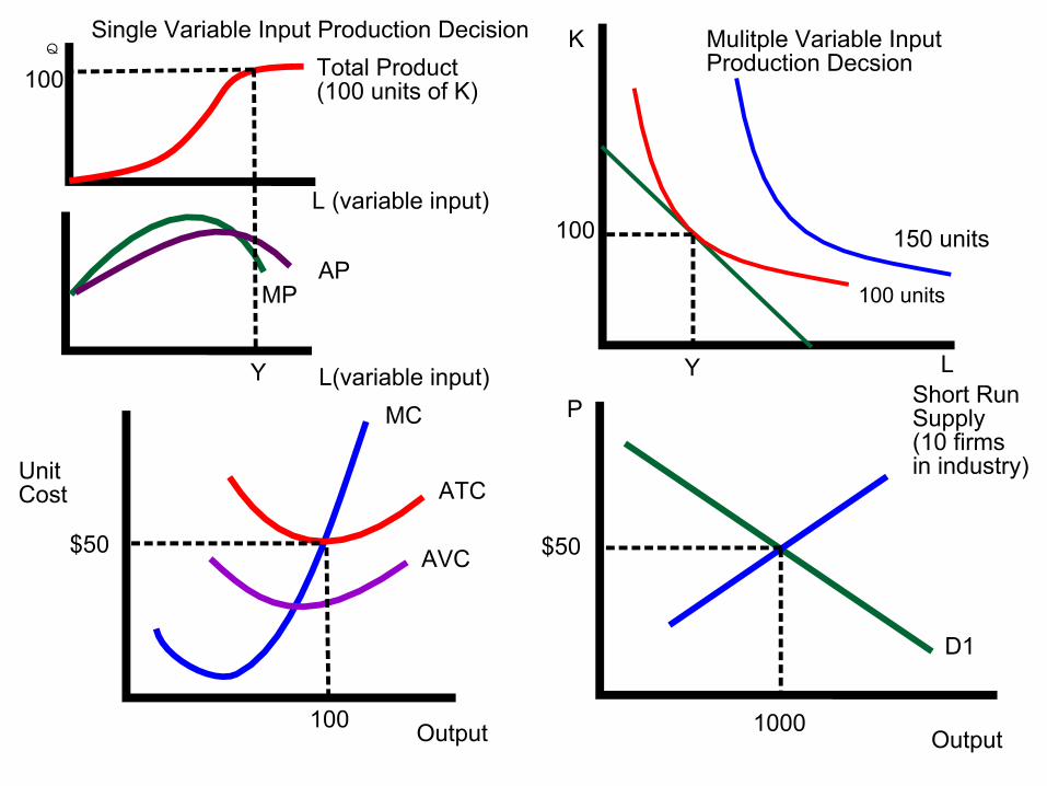
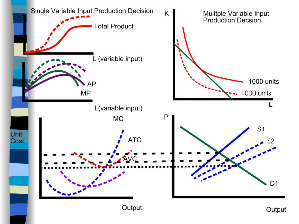
Begin with the Multiple Variable Input Production Decision.
How will the technological change effect the iso-output curve for a given quantity?
It will shift it in—the same output can be produced with less capital and labor.
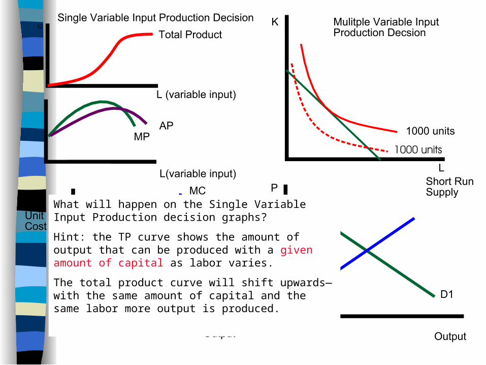
What will happen on the Single Variable Input Production decision graphs?
Hint: the TP curve shows the amount of output that can be produced with a given amount of capital as labor varies.
The total product curve will shift upwards—with the same amount of capital and the same labor more output is produced.

Given the shift in the TP curve, what will happen to the MP and AP curve?
The slope of the TP has generally increased so MP has increased at each point.
Also, because more out put is being produced at each combination of capital and labor, the AP curve will also shift upward.
What will happen to the unit cost curves—ATC, AVC, and MC?
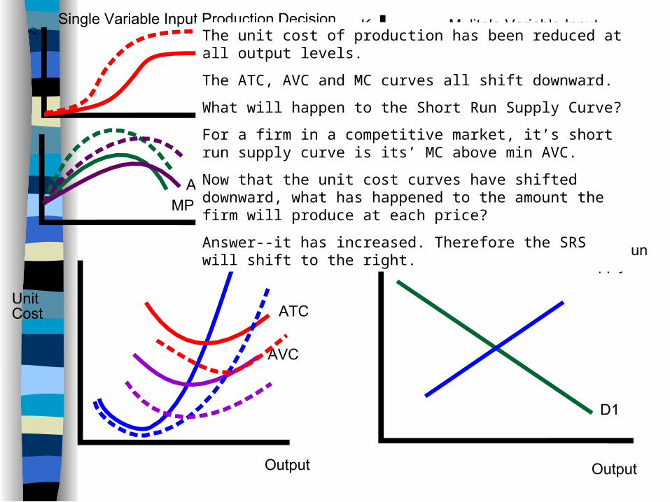
The unit cost of production has been reduced at all output levels.
The ATC, AVC and MC curves all shift downward.
What will happen to the Short Run Supply Curve?
For a firm in a competitive market, it’s short run supply curve is its’ MC above min AVC.
Now that the unit cost curves have shifted downward, what has happened to the amount the firm will produce at each price?
Answer--it has increased. Therefore the SRS will shift to the right.

The shift of the SRS to S2 has increased the amount produced and lowered the price.
What will happen in the long run?
Are the existing firms earning a profit at the new short run equilibrium price?

At the new price, the existing firms are earning a profit so there will be entry of new firms.
As new firms enter the market, the short run supply curve will continue to shift out until the equilibrium price is equal to the new min ATC.

Notes for Exam
Calculator allowed. No blue book. Bring pen.