Economics 407: Topics in Macroeconomics Problem Set #1: Answers

These problems are due on Tuesday, January 28th

.

1. Consider the following equations describing the supply-side of a macroeconomy:

21

L800Y = 2

s

P

WL

=

Here Y represents total output, L the quantity of labor, Ls labor supply, W the nominal wage, and

P the price level.

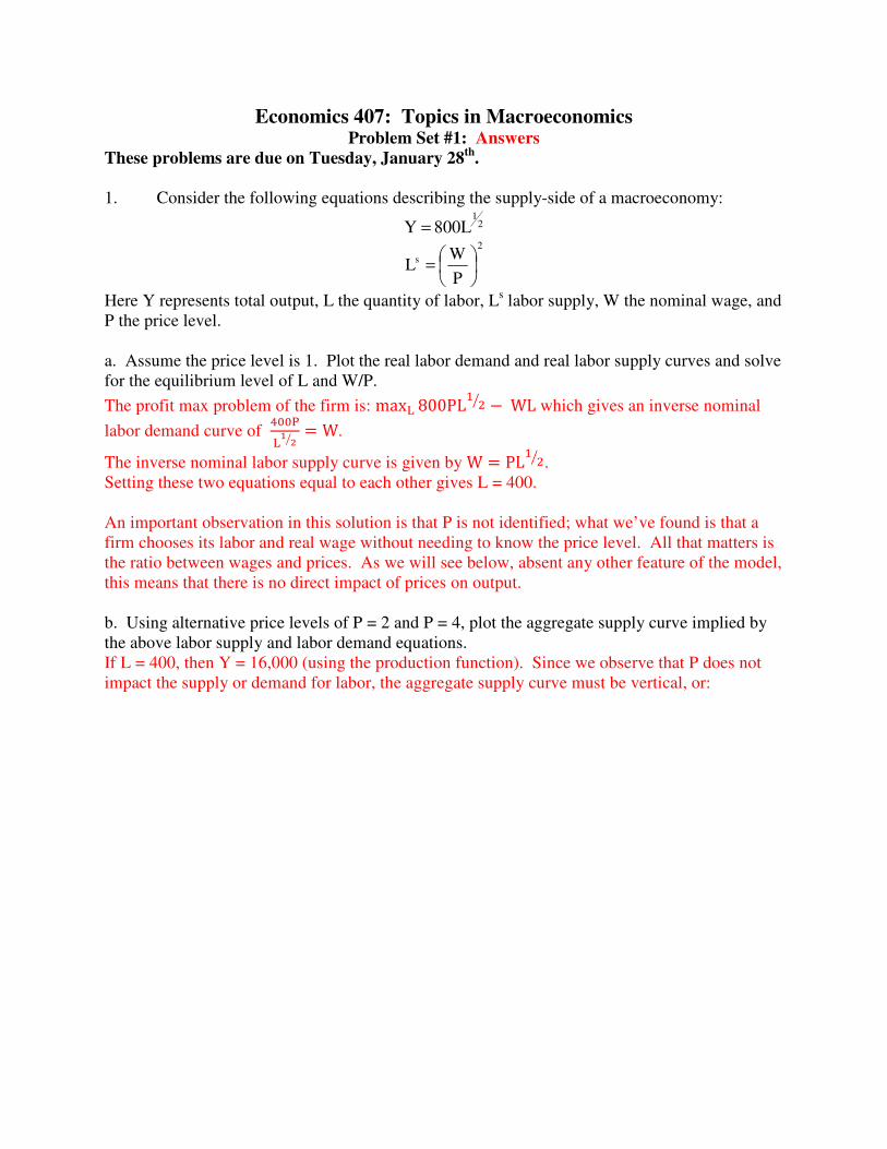
a. Assume the price level is 1. Plot the real labor demand and real labor supply curves and solve

for the equilibrium level of L and W/P.

The profit max problem of the firm is: max� 800PL� − WL which gives an inverse nominal

labor demand curve of ����

��

��= W.

The inverse nominal labor supply curve is given by W = PL� .

Setting these two equations equal to each other gives L = 400.

An important observation in this solution is that P is not identified; what we’ve found is that a

firm chooses its labor and real wage without needing to know the price level. All that matters is

the ratio between wages and prices. As we will see below, absent any other feature of the model,

this means that there is no direct impact of prices on output.

b. Using alternative price levels of P = 2 and P = 4, plot the aggregate supply curve implied by

the above labor supply and labor demand equations.

If L = 400, then Y = 16,000 (using the production function). Since we observe that P does not

impact the supply or demand for labor, the aggregate supply curve must be vertical, or:

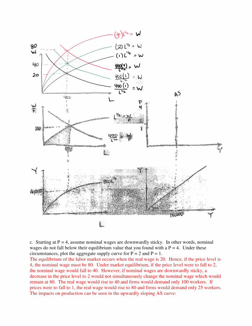
c. Starting at P = 4, assume nominal wages are downwardly sticky. In other words, nominal

wages do not fall below their equilibrium value that you found with a P = 4. Under these

circumstances, plot the aggregate supply curve for P = 2 and P = 1.

The equilibrium of the labor market occurs when the real wage is 20. Hence, if the price level is

4, the nominal wage must be 80. Under market equilibrium, if the price level were to fall to 2,

the nominal wage would fall to 40. However, if nominal wages are downwardly sticky, a

decrease in the price level to 2 would not simultaneously change the nominal wage which would

remain at 80. The real wage would rise to 40 and firms would demand only 100 workers. If

prices were to fall to 1, the real wage would rise to 80 and firms would demand only 25 workers.

The impacts on production can be seen in the upwardly sloping AS curve:

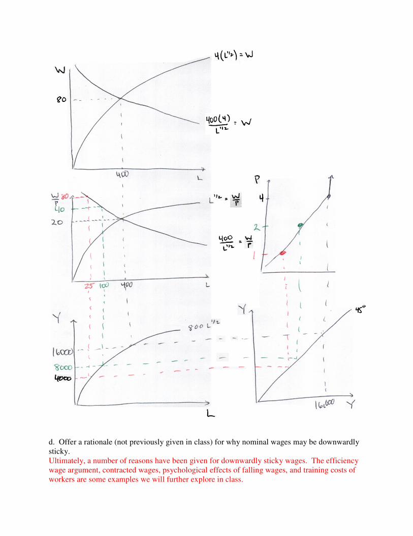
d. Offer a rationale (not previously given in class) for why nominal wages may be downwardly

sticky.

Ultimately, a number of reasons have been given for downwardly sticky wages. The efficiency

wage argument, contracted wages, psychological effects of falling wages, and training costs of

workers are some examples we will further explore in class.

2. Consider the following equations representing a typical Keynesian model of aggregate

demand:

Y = C + I + G

C = a + b(Y – T)

I = c – eR

G = g

Where lower case letters represent parameters and R represents the real interest rate.

a. Using the total derivative technique discussed in class, find dg

dY. Think carefully about the

IS/LM diagram, what did you just find?

We know that because every expenditure must be another person’s income, Y = C + I + G + NX.

Since NX = 0 in this case, it must be that Y = C + I + G or: Y = a + b(Y – T) + c – eR + g.

Taking the total derivative of this expression gives:

dY = da + db(Y – T) + bdY – bdT + dc – Rde – edR + dg

Since the question asks for dY/dg, we can assume that there are no other changes in any of the

variables. Variables that do not change necessarily have values d(·) = 0. In this case, that leaves:

dY = bdY + dg. Solving for dg

dY gives

bdg

dY

−

=

1

1, or what we call the spending multiplier.

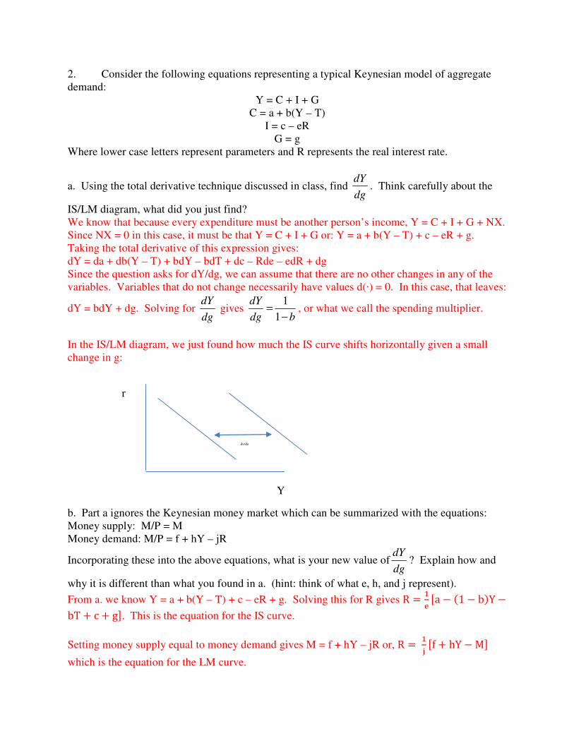
In the IS/LM diagram, we just found how much the IS curve shifts horizontally given a small

change in g:

b. Part a ignores the Keynesian money market which can be summarized with the equations:

Money supply: M/P = M

Money demand: M/P = f + hY – jR

Incorporating these into the above equations, what is your new value ofdg

dY? Explain how and

why it is different than what you found in a. (hint: think of what e, h, and j represent).

From a. we know Y = a + b(Y – T) + c – eR + g. Solving this for R gives R =

��a − �1 − b�Y −

bT + c + g!. This is the equation for the IS curve.

Setting money supply equal to money demand gives M = f + hY – jR or, R =

"�f + hY − M!

which is the equation for the LM curve.

r

Y

dy/dg

Setting the IS and LM equations equal gives:

��a − �1 − b�Y − bT + c + g! =

"�f + hY − M!

Solving for Y gives:

Y = ja − jbT + jg − ef + eM

eh + j�1 − b�

From this equation it is clear that: dY

)*=

j

eh + j�1 − b�=

1eh

+� + �1 − b�

The introduction of the LM curve changes our estimate of the spending multiplier because

changes in spending how have an equilibrium impact on interest rates which has a “feedback”

effect on income. In this case, because eh/j > 0, the spending multiplier is smaller than we first

estimated in part a. The basic story is as follows:

An increase in government spending stimulates income and others to consume (the traditional

spending multiplier story). However, as incomes rise, individuals begin to hold money

(governed by the parameter h) which shifts the money demand curve upward. As money

demand increases, so do interest rates (governed by parameter j). As interest rates rise,

investment spending falls (governed by parameter e) and this fall reduces government spending’s

impact on Y.

c. Some economists argue that Investment is a positive function of income (higher incomes

might induce firms to increase spending on capital). Replace the Investment demand equation

with I = c – eR + mY where m could be thought of as the marginal propensity to invest and is

constrained to be larger than zero and m + b < 1. Solve for dg

dY and explain why it differs from

what you found earlier.

Under this setup, the new IS curve is R =

��a − �1 − b −m�Y − bT + c + g!

Setting this equal to the LM curve gives an equilibrium quantity of Y as:

Y = ja − jbT + jg − ef + eM

eh + j�1 − b − m�

The spending multiplier is now: ,-

./=

"

�01"�23�=

�0

4� 1�2325�.

Notice, this is larger than the one found in part c.

In this case, an increase in government spending raises income through the traditional multiplier

process AND as income grows, so does investment (at rate m). This increase in investment also

raises income and perpetuates the increased growth in Y.

d. Returning to the economy described by parts A and B, I would like you to think through a

different argument that mitigates the spending multiplier you found in parts a, b and even c. The

following is termed “Ricardian Equivalence.” We will completely develop the Ricardian

Equivalence argument during Interlude #2 of this course. For now, consider a government who

wishes to increase spending by one dollar. Even absent the interest rate effect found in part B,

one might imagine that tax payers realize that higher government spending today requires

increased future taxes (either immediately to pay off the higher spending or in the future to pay

off the bonds associated with that spending). As a result, consumers increase their savings

immediately so as to be prepared for those future taxes. One might model this as:

C = a + b(Y – T) – qG

where 0 < q ≤ 1 is a parameter that indicates how much consumers decrease their spending for

each additional dollar spending by the government. Alternatively, one might imagine that

government purchases serve as substitutes for household purchases at rate q.

Solve for dg

dY if C = a + b(Y – T) – qG. What happens to the spending multiplier as q goes to

one. Explain.

Under this scenario, the new IS curve is given by R =

��a − �1 − b�Y − bT + c + �1 − q�g!.

Setting this IS curve equal to the LM curve and solving for Y, gives

Y = ja − jbT + j�1 − q�g − ef + eM

eh + j�1 − b�

In this case, dY

)*=

j�1 − q�

eh + j�1 − b�=

1 − qeh

+� + �1 − b�

An increase in government spending leads to a smaller increase in output because, in this case,

government spending substitutes for consumption; an increase in g causes a partial reduction in

C.