Embed Size (px)
DESCRIPTION
Economics study book USQ
Citation preview
ECO1000
EconomicsFaculty of Business and Law
Study book
Published byUniversity of Southern QueenslandToowoomba Queensland 4350Australiahttp://www.usq.edu.au
© University of Southern Queensland, 2013.2.
Copyrighted materials reproduced herein are used under the provisions of the Copyright Act 1968 as amended, or as a result of application to the copyright owner.
No part of this publication may be reproduced, stored in a retrieval system or transmitted in any form or by any means electronic, mechanical, photocopying, recording or otherwise without prior permission.
Produced by Learning Resources Development using the ICE Publishing System.
Table of contentsPage
Module 1 – Introduction to economics 1Learning objectives 1Learning resources 1
Text 1Essential 1
1.1 Introduction 11.1.1 The economic way of thinking 21.1.2 The language of economics 3
1.2 Thinking like an economist 31.2.1 Economic models 4
1.3 Using graphs in economics 51.4 Production economics 6
1.4.1 Scarcity and opportunity cost 6Summary 9
Module 2 – How the market works 11Learning objectives 11Learning resources 11
Text 11Essential 11
2.1 Introduction 112.2 Tools of analysis: demand 12
2.2.1 The concept of demand 122.2.2 The demand curve 122.2.3 The downward-sloping demand curve 142.2.4 Movements along and shifts of the demand curve 142.2.5 Reasons for the demand curve to shift 15
2.3 Tools of analysis: supply 152.3.1 The concept of supply 152.3.2 A single firm’s supply 162.3.3 Market supply 172.3.4 Movements along and shifts of the supply curve 182.3.5 Reasons for the supply curve to shift 18
2.4 Tools of analysis: market equilibrium 182.5 Elasticity 20
2.5.1 Introduction 202.5.2 The concept of elasticity 212.5.3 Price elasticity of demand 212.5.4 Cross-price elasticity of demand 212.5.5 Income elasticity of demand 212.5.6 Price elasticity of supply 22
2.6 Economic efficiency and market failure 232.6.1 Consumer and producer surplus and economic efficiency 232.6.2 Price floors and price ceilings 242.6.3 The economic impact of taxes 24
Summary 25
Module 3 – Firms and market structure 27Learning objectives 27Learning resources 27
Text 27Essential 27
3.1 Introduction 273.2 The concept of cost revisited 283.3 The short run production function 293.4 Short run cost functions 303.5 Long run average cost 303.6 The model of perfect competition 32
3.6.1 Introduction 323.6.2 The perfectively competitive model: in the short run 323.6.3 The entry and exit of firms in the long run and efficiencies in perfect competition 32
3.7 Monopoly markets 353.7.1 Monopoly model 353.7.2 Economic efficiency and government regulation in monopoly market 36
Summary 37
Module 4 – Macroeconomic Foundations 39Learning objectives 39Learning resources 39
Text 39Essential 39
4.1 Introduction 404.2 GDP measures total production 40
4.2.1 Measuring the size of the total production 404.2.2 The circular flow model of an economy 414.2.3 Economic growth 42
4.3 Unemployment and inflation 434.3.1 Unemployment 434.3.2 Inflation 44
4.4 The business cycle 454.5 Aggregate demand and aggregate supply 45Summary 47
Module 5 – Monetary and Fiscal policy 49Learning objectives 49Learning resources 49
Text 49Essential 49
5.1 Introduction 505.2 Money, banks and the Reserve Bank of Australian 515.3 Monetary policy 525.4 Fiscal policy 54Summary 55Appendix 5.1 (optional reading, and not examinable) 59
Epilogue: brief review of selected schools of thought in economics 59
ECO1000 – Economics 1
Module 1 – Introduction to economics
Learning objectivesOn successful completion of this module, you should be able to:
● discuss the three important ideas: people are rational; people respond to incentives; optimal decisions are made at the margin
● understand the issues of scarcity, and trade-offs
● understand the concepts of opportunity cost, the difference between centrally planned economy and market economy, and the issues associated with efficiency and equity
● understand the role of models in economic analysis
● understand normative and positive analysis, and distinguish between microeconomics and macroeconomics
● apply graphical techniques in economic analysis and understand their interpretations
● apply the model of the ‘production possibilities frontier’ to illustrate the concepts of opportunity cost and economic growth
● understand comparative advantage and explain how it is the basis for trade
● explain the basic idea of how a market system works.
Learning resources
TextHubbard, Garnett, Lewis, and O'Brien, 2013, Economics, chapters 1 and 2 ; appendix to chapter 1.
EssentialStudy book: module 1.
1.1 IntroductionThis module introduces you to the study of the social science of economics. As a social science, economics provides an orderly approach to theory development, to the construction and testing of models, and to the analysis of economic policy. Practical economics seeks to focus the power of reason on the economic issues of our times.
© University of Southern Queensland
2 ECO1000 – Economics
When starting the study of economics, you have to learn the assumptions and language of this new way of thinking. One of the difficulties with learning economics is that it can take some time to get used to this approach to everyday life. Some people are fortunate, in that they grasp the principles quite quickly; however, for most, it takes some time. Therefore, the course team believes that it is best to start slowly with a few concepts and then add to them as you work through the course.
As with learning another language, you first learn very basic words, then you move to phrases, and then you ‘learn sentences’. Finally, you learn how to be ‘grammatically accurate’; but this can take many years. Due to time constraints, this course can only take you to the very early stage of ‘learning sentences’ or, in this case, applying concepts.
1.1.1 The economic way of thinkingEconomics provides a set of analytical tools, but it is also a way of thinking. In this course we are showing you some of those basic tools and trying to encourage you to understand the ‘economic way of thinking’. This way of thinking is characterised by a ‘language’ in which words have a meaning specific to economics. As with any language, you need to understand the terms and their definitions. However, economics is most importantly a particular way of looking at individual, group and national behaviour. In other words, economics provides another way of looking at our domestic lives, our working lives and national and international politics. Some economists have argued that even marriage, crime and human life can be analysed in terms of economic choices.
It may help you to understand the main concepts in this course if you keep posing the question ‘how would an economist interpret this?’ It may also help to relate the concepts to everyday situations; indeed, newspaper discussions on economics can provide some good material for consideration. However, remember that this is an introductory course, and we use a lot of assumptions to simplify the concepts for teaching purposes. Therefore, you cannot always get the ideas and examples to exactly conform to real-world situations. Try to think of the concepts presented at this level as being limited to the illustration of general tendencies.
An important part of the language of economics is maths. This course has been designed to de-emphasise the maths (believe it or not), but some knowledge of maths is useful. Apart from the use of simple algebraic formulae in economics, there are various ‘tools’ to show data and to illustrate or represent concepts. Economic data is presented in three main ways:
● descriptive prose (written work). Economics, as with any social science, relies heavily on descriptions of what has happened and what is happening
● tables of numbers that can be used to identify trends or points of note. Tables are used throughout the text and it is important that you learn to interpret information from them
● graphs of key indicators and measures, usually over time or in relation to each other. These are usually based on tables and are really a variation of the above.
Most of the course is based on written explanation, as you would expect when learning a social science. While there are other ways of representing economic ideas, this remains one of the most fundamental. Being able to explain an idea or concept is still a real test of understanding. That is why we use assessment, such as the written assignment and the extended response questions, in the exam.
© University of Southern Queensland
ECO1000 – Economics 3
There are also algebraic equations, where symbols are used to represent variables. These are occasionally used to calculate real numbers, for example calculating the size of an economy, but they are often symbolic. That is, the equation is just a shorthand way of explaining a relationship.
While the obvious focus of the course is on content, we also want you to develop skills in description and interpretation. Therefore, it is very important that you take the opportunity to develop the capacities to interpret data and to identify concepts as they are variously expressed.
1.1.2 The language of economicsYou will come across many terms used throughout this course and also in your career. Economics is the language used in politics, the media, and in business. It will be everywhere in your daily lives. The level of wages you receive, your job security and the interest you pay on a home loan are all indicators of economic activity and they will all be discussed in economic terms. If you want to interpret what is happening to you, you must be able to speak the language. You may find it useful to refer frequently to the glossary of terms at the back of the text.
1.2 Thinking like an economistEconomists get ‘bad press’. At best they are often portrayed as people who deal entirely with the abstract, having little or no experience of the ‘real world’. At worst, they are portrayed as hard-hearted, narrow people, seeking to reduce human activities to monetary values, and proposing policies that add to human misery. However, many economists are engaged with questions of poverty, development, fairness, distribution, the environment and so on and they do wish to make the world a better place, though often disagreeing with each other about how that might be achieved. At the heart of the activity of the economist lies the development of theories and models. In developing these theories and models, economists have sought to bring a particular way of thinking, which is really common sense plus careful reasoning and the use of data, to make the world a better place. It is a difficult task.
People must make choices as they try to attain their goals. These choices reflect trade-offs people make because we live in a world of scarcity; although our wants are unlimited, the resources available to satisfy our wants are limited. Economic models are simplified versions of some aspects of economic life. Economists construct models and use them to analyse economic issues. Economics focuses on the decisions buyers and sellers make through markets. Economists assume people (1) are rational, (2) respond to economic incentives, and (3) make optimal decisions at the margin.
Economists often focus on decision-making ‘at the margin’ on the grounds that when making choices, economic agents (be they consumers, firms or governments) focus on the benefits and costs associated with the extra, or marginal, activity. For example, when considering whether or not to buy another pizza, a consumer would calculate (however roughly) the marginal cost and the marginal consumption benefit; a business when considering whether or not to hire another saleswoman would calculate the marginal cost of employing the worker and the marginal revenue to be gained from her services; and a government when considering whether or not to build another hospital, would consider the extra costs and extra benefits
© University of Southern Queensland
4 ECO1000 – Economics
from constructing and running another hospital. For economists, economic agents will only make decisions to undertake the extra activity if the marginal benefit is equal to, or greater than, the marginal cost. Try a little introspection on this point; ask yourself if this what ‘goes through your mind’ when you make consumption choices (for example, to have another drink; to buy another loaf of bread; or to spend an extra week on holiday).
Each society faces the economic problem of having a limited amount of resources, and so can produce a limited amount of goods and services. Each society faces trade-offs, particularly when answering three questions: (1) What goods and services will be produced? (2) How will the goods and services be produced? (3) Who will receive the goods and services produced? Societies organise their economies in two main ways to answer these questions. A society can have a centrally planned economy characterised by extensive government decision making. Or a society can have a market economy in which the decisions of households and firms interacting in markets allocate resources. Most developed countries have predominately market economies with some central government regulation or control. Market economies tend to allocate resources more efficiently than do centrally planned economies, but efficient outcomes may not be perceived as fair. Determining what is a fair or equitable outcome calls for the application of normative economic analysis – what ought to be. Positive economic analysis is concerned with what is. While most or all economists can agree on the results of positive economic analysis, they may disagree widely on normative economic issues.
Microeconomics is the study of how individual choices are made by households, business firms, and government. Macroeconomics is the study of the economy as a whole.
1.2.1 Economic modelsIt is important to realise that economics is a social science, not a natural science. In other words, the ‘economy’ is not like a mechanical system, even though some economists and politicians speak as if it were. Economics is about the study of human activity in relation to the production, distribution and exchange of goods and services. The behaviour of humans is not always, or perhaps ever, scientifically predictable; however, economists have developed a range of techniques for trying to make sense of economic activity.
The ‘real’ world, that is, the world in which you live, is very complicated. Consequently, economists have to use ‘pretend economies’ to simplify it. These pretend economies, or models, are simplifications of the real world. From the models, you can derive general propositions about the relationships and the behaviour of groups of individuals. Such propositions are developed using economic theories. Remember, you are taking an introductory course and simplification is required; don’t try to make everything fit neatly into real world situations.
Theoretical reasoning, followed by data analysis, helps economists to explain the operation of the economy and to develop solutions to economic problems. An economic model cannot be so simple that it is completely unrealistic, but neither must it be so complex that important interrelationships are lost in the detail.
Finally, while the models and graphs might seem scientific and objective, it is important to note that they are very much based on certain assumptions about how people do, or will, behave in particular circumstances. When studying a model, always look for the assumptions, be they explicit or implicit, the logical reasoning used, and the conclusions reached.
© University of Southern Queensland
ECO1000 – Economics 5
Reading activity 1.1Study chapter 1 of the text (Hubbard et al.).
Make sure that you can:
● Discuss the three important economic ideas: people are rational; people respond to incentives; optimal decisions are made at the margin
● explain the social science of economics as the study of scarcity and choice
● understand the role of models in economic analysis
● distinguish between ‘positive’ and ‘normative’ economics
● distinguish between microeconomics and macroeconomics.
Learning activity 1.1NB: This is the essential set of exercises. If you have additional time, you should practise the quizzes and tests in MyEconlab (Check the StudyDesk on how to access MyEconlab).
1.1.1 Answer Review Questions 1-10 and Problems and Applications 2, 3, 4, 5, 11, 12, 14, 15, 16, 17, 20 at the end of chapter 1 (check your answers with those from the StudyDesk).
1.3 Using graphs in economicsIt is common practice in economics to use graphs to illustrate relationships among economic variables and to work out the effects of changes in economic circumstances. Accordingly, it is necessary that we pause to ensure that the essential aspects of graphical analysis are understood.
Reading activity 1.2Study Appendix to chapter 1 of the text (Hubbard et al.).
Make sure that you can:
● plot graphs of economic data to show the relationship between two variables
● use graphs to illustrate positive and negative relationships between economic variables
● calculate the slopes of a straight line and a curved line
© University of Southern Queensland
6 ECO1000 – Economics
Learning activity 1.2NB: This is the essential set of exercises. If you have additional time, you should practise the quizzes and tests in MyEconlab.
1.2.1 Answer all questions in 'Problems and Applications' for the appendix to chapter 1 (check your answers with those from the StudyDesk).
1.4 Production economics
1.4.1 Scarcity and opportunity costIn our previous study, we introduced economics as the science of scarcity and choice. The problem of scarcity is often developed in terms of the three fundamental economic questions: ‘what to produce’, ‘how to produce it’, and ‘for whom to produce it’? In this presentation of the problem of scarcity, two very important economic concepts emerge: ‘opportunity cost’ and ‘marginal analysis’.
Opportunity costOne of the most important concepts in economics is that of opportunity cost. This is a concept that has application in many aspects of our lives. Indeed, for every action we undertake, there is an opportunity cost (or something foregone). Every time you spend time or money, you make a choice and you forego all other opportunities. For example, if you go out in the evening to socialise, you forego the opportunity to watch television, or to study or to spend time with your family. You cannot claim you will catch up on those things later, because of the time factor. In economics, there is always scarcity. For humans, time is limited and the hours used cannot be recaptured. It is the same with spending. If you buy movie tickets, you cannot use that money for a meal, savings or for the purchase of DVD. You are making choices all the time and the cost is to be thought of in terms of what has been foregone. Accordingly, opportunity cost may be defined as:
The value of that which must be given up to acquire or achieve something.
Opportunity cost is therefore expressed in the terms of what is ‘given up’. Strictly speaking, opportunity cost is to be thought of in terms of the next best option that has been given up.
Here is an example:
● A visit to the movies. You go to the movies instead of studying. The financial cost is the entry fee (say $10) but an additional opportunity cost of going to the movies is the foregone 2 hours of study. Thus, the opportunity cost of going to the movies is $10 + the value of 2 hours of study.
© University of Southern Queensland
ECO1000 – Economics 7
Production possibilities frontier (PPF)Illustrating the concept of opportunity cost, the production possibility frontier is a valuable tool used to examine the consequences of production initiatives, changes in the resource mix and developments in technology. It is our first example of an economic model.
Production possibility frontiers may be used to graphically demonstrate the impact of inefficiency within the economy. In Australia, during the 1980s and the 1990s, an appreciation of this inefficiency led to the introduction of widespread industrial reform measures designed to deliver better work practices and, consequently, improvements to net community welfare. These changes, taken together, became known as microeconomic reform.
The PPF delineates what it is possible to produce from what it is not possible to produce. Individuals have PPFs in relation to particular goods that they can produce. That is, each of you has a limit to what you could produce, within a particular time frame, whether that is pages of typing, sales of goods or house painting. In similar fashion, we can think of the PPF for any economy. Given a number of assumptions, the PPF for an economy shows the combinations of goods that can be produced with full and efficient use of available resources.
The PPF is an example of an economic model that has been constructed to show the key relationships that underlie production in any economy. It is usually represented in terms of a graph with two goods shown on the axes, and is shown as a ‘bowed outwards’ curve. Essentially, it shows the production ‘boundary’ for an economy and the fact that, if the economy is producing efficiently, it can only produce more of one good by giving up increasing amounts of the other good (the ‘law of increasing opportunity costs’).
Note that, conceptually, we can apply the PPF to many resource-use questions (for example, the production of ‘defence’ or ‘peacetime’ goods; the production of a ‘clean environment’ or ‘ordinary’ industrial output; and the production of ‘health goods’ or ordinary consumer goods).
Note, also, that we may consider a change (such as an increase in the output of one good at the expense of the output of another) that is modelled by a movement along a given PPF, or a change that is modelled by a shift of the PPF (such as a change in technology that enables more of all goods to be produced from a given quantity of resources.
Specialisation and the gains from tradeThe logic that flows from the concept of opportunity cost is that if we, as individuals, business, people and citizens, want economic efficiency and to maximise the outcomes of our economic efforts, then both individuals and nations should ‘specialise’. Specialisation is the cornerstone of the modern economy. The principle is that it is theoretically more efficient to specialise in production and then exchange or trade, than to try and be fully self-sufficient.
The argument that nations gain by specialising in production and trading is based on the theory of comparative advantage. Essentially, this says that a country with a comparative advantage in the production of a good or service should specialise in the production of that good or service and exchange it for goods and services from other countries. A country is
© University of Southern Queensland
8 ECO1000 – Economics
said to have a comparative advantage when it has a lower opportunity cost of production than do its trading partners.
It is important to distinguish between ‘comparative advantage’ and ‘absolute advantage’. Whereas comparative advantage exists when a country has a lower opportunity cost of production, absolute advantage refers to the situation in which a country has a lower absolute cost of production in terms of resources used.
The market systemHubbard et al. (2013, pp. 40–45) have a good discussion of the following basic concepts. It is essential to understand them before we move on to modules 2 and 3.
A market is a group of buyers and sellers of a good or service and the institution or arrangement by which they come together to trade. Product markets are markets for goods – such as computers – and services – such as medical treatment. Factor markets are markets for the factors of production, such as labour, capital, natural resources, and entrepreneurial ability.
A free market is a market with few government-imposed restrictions on how a good or service can be produced or sold, or on how a factor of production can be employed.
The market mechanism refers to the inherent forces in the market that will allocate resources in a way that maximises consumer satisfaction. The assumption is that individuals are rational and self-interested. Therefore producers will produce and sell what consumers want to buy, so that the producers can maximise their own profits. These inherent forces are what Adam Smith referred to as the ‘invisible hand’ of the market.
The price mechanism is the signalling device between consumers and producers; if consumers are willing to pay a higher price due to strong demand, this will signal producers to supply more; if demand for a product is low at the current price, the product won’t sell and producers will need to lower the price.
Entrepreneurs are an essential part of a market economy. An entrepreneur is someone who operates a business, bringing together the factors of production – labour, capital, and natural resources – in order to produce goods and services. Entrepreneurs often risk their own funds to start businesses and organise factors of production to produce those goods and services consumers want.
Reading activity 1.3Study chapter 2 of the text (Hubbard et al.).
Make sure that you can:
● define the term ‘opportunity cost’
● explain and apply the concept of the ‘production possibilities frontier’
● distinguish between the concepts of ‘absolute’ and ‘comparative’ advantage
● use the concept of the production possibilities frontier, and theory of comparative advantage, to explain the gains from trade.
● Explain the basic idea of how a market system works
© University of Southern Queensland
ECO1000 – Economics 9
Learning activity 1.3NB: This is the essential set of exercises. If you have additional time, you should practise the quizzes and tests in MyEconlab.
1.3.1 Answer Review Questions 1-10 and Problems and Applications 1, 2, 3, 4, 5, 6, 8, 9, 10, 11, 12, 14, 15, 16, 17, 19 at the end of chapter 2 (check your answers with those from the StudyDesk).
SummaryThis module introduced the study of economics and explored briefly some of the essential concepts and methods used by economists in their professional work. Economists seek to use the economic way of thinking to develop answers to a wide range of questions arising from the general problem of relative scarcity. Its methods are applicable to the analysis of the choices of households, businesses and governments. They are applicable, also, at the level of a region, a nation, or the world.
In this module, we explored the economic way of thinking, the use by economists of graphical analysis, a number of key concepts, and the model of the production possibilities frontier. We saw how this model enabled us to consider the decision problem faced by a country (or a person or business at the micro level) as it sought to use its resources efficiently. We saw also that the model can be used to explain the gains that a country may capture by engaging in specialisation and trade. We also acknowledged that Entrepreneurs, those who own and operate businesses, are critical to the working of a market system. They produce goods and services consumers want and decide how these goods and services should be produced to yield the most profit.
We will introduce a number of additional concepts and models in subsequent modules as we develop our understanding of the importance of economics for the welfare of people.
© University of Southern Queensland

10 ECO1000 – Economics
© University of Southern Queensland
ECO1000 – Economics 11
Module 2 – How the market works
Learning objectivesOn successful completion of this module, you should be able to:
● explain the concepts of demand, supply, and market equilibrium
● explain the concept of elasticity
● calculate and interpret price, income and cross-price elasticity of demand
● calculate and interpret price elasticity of supply.
● understand the concepts of consumer surplus and producer surplus
● use demand and supply graphs to analyse the economic impact of price ceiling and price floors
● use demand and supply graphs to analyse the economic impact of taxes
Learning resources
TextHubbard et al., 2013, Economics, chapters 3, 4 and 5.
EssentialStudy book: module 2.
2.1 IntroductionThis module introduces the well-known economic concepts (tools) of supply and demand, and their use in market analysis. The ‘supply-demand’ model of a market provides us with important insights into the use of resources in a market economy, largely a response to the signals conveyed to decision-makers by prices in an economy. Using this model, we are able to predict the general direction of changes in prices and quantities resulting from changes in the market-place (for example, those arising from the imposition of a sales tax on goods purchased by consumers, or from the payment of a subsidy to producers).
Before the ‘market’ model can be used, it is necessary to have a sound grasp of the concepts of supply and demand and of a measure of responsiveness to a given change in the market, known as elasticity.
© University of Southern Queensland
12 ECO1000 – Economics
Once the mechanics of the model have been mastered, you will find that you can use it to analyse contemporary economic issues, for example, the move to deregulate the Australian labour market. Our focus in this module is on the operation of particular markets (such as the market for unleaded petrol); this is the field of microeconomics as distinct from macroeconomics.
In the previous module, we introduced a number of concepts used by economists and also spent some time looking at what is means to ‘think like an economist’. In this module, we continue that pattern when we turn our attention to the economic analysis of markets.
We are aware, of course, that markets and trading in markets are as old as human history. Some markets are readily observable, such as those for fruit and vegetables, while others are quite obscure, such as those for futures and share options. Despite the legality, or otherwise, of markets, we should be able to apply our tools of market analysis to any market situation.
Our aim is to understand how markets work and to predict the direction of change in market prices and quantities traded that are likely to follow some change in the economy. For example, in Australia at the moment, many people are very concerned about the rising price of fuel for motor vehicles. As economists, we would like to use the tools of market analysis to predict the likely change in the price of fuel over the next month, or year. In this module, we will see how economists develop their predictions.
2.2 Tools of analysis: demand
2.2.1 The concept of demandEconomists define market demand as the set of possible prices per unit of the good and the quantities that would be demanded at each of those prices (other things remaining the same; the ‘ceteris paribus’ assumption). If we knew the set of prices and associated quantities, we could show this information in a table, or plot it to represent a market demand curve (more specifically, the price demand curve). This is usually drawn as a downward-sloping curve.
Individual demand is defined in the same way. It is the set of possible prices and the associated quantities demanded by a consumer (other things remaining equal: that is, ceteris paribus). As for market demand, we an represent individual demand in a table of data or by a plot of the price-quantity information contained in the table.
2.2.2 The demand curveSuppose we have the following price and quantity demanded information for a consumer. Table 2.1 is Peter’s demand for hamburgers (ceteris paribus).
Table 2.1: Peter’s demand for hamburgers
Price per hamburger ($) 1.50 2 2.50 3 3.50 4 4.50 5 5.50
Quantity demanded/wk 9 8 7 6 5 4 3 2 1
© University of Southern Queensland
ECO1000 – Economics 13
This table shows the quantity demanded by Peter at each and every possible price. That is, if the price were $1.50, he would buy nine hamburgers per week and so on. Note that this information tells us what Peter would purchase if the price were, $1.50, $2.00 etc., and that the ceteris paribus assumption applies.
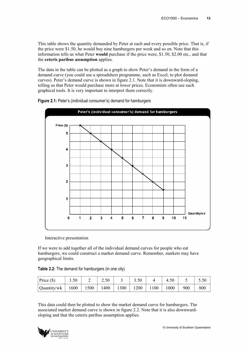
The data in the table can be plotted as a graph to show Peter’s demand in the form of a demand curve (you could use a spreadsheet programme, such as Excel, to plot demand curves). Peter’s demand curve is shown in figure 2.1. Note that it is downward-sloping, telling us that Peter would purchase more at lower prices. Economists often use such graphical tools. It is very important to interpret them correctly.
Figure 2.1: Peter’s (individual consumer’s) demand for hamburgers
Interactive presentation
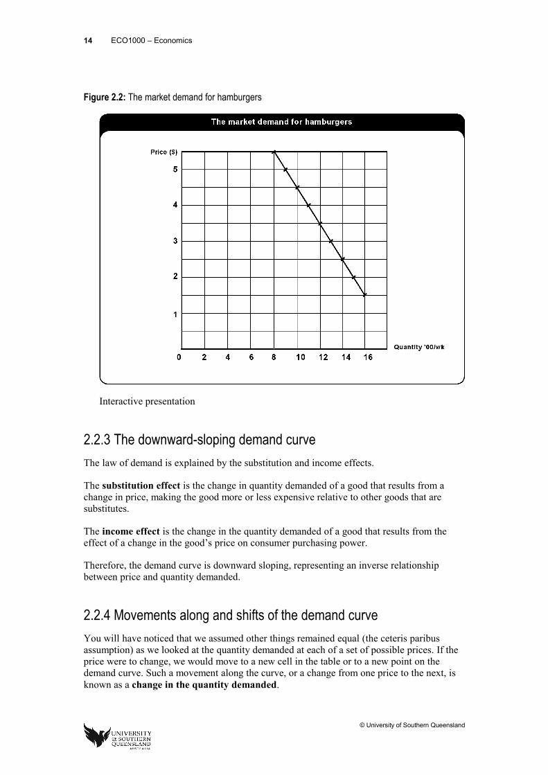
If we were to add together all of the individual demand curves for people who eat hamburgers, we could construct a market demand curve. Remember, markets may have geographical limits.
Table 2.2: The demand for hamburgers (in one city)
Price ($) 1.50 2 2.50 3 3.50 4 4.50 5 5.50
Quantity/wk 1600 1500 1400 1300 1200 1100 1000 900 800
This data could then be plotted to show the market demand curve for hamburgers. The associated market demand curve is shown in figure 2.2. Note that it is also downward-sloping and that the ceteris paribus assumption applies.
© University of Southern Queensland
14 ECO1000 – Economics
Figure 2.2: The market demand for hamburgers
Interactive presentation
2.2.3 The downward-sloping demand curveThe law of demand is explained by the substitution and income effects.
The substitution effect is the change in quantity demanded of a good that results from a change in price, making the good more or less expensive relative to other goods that are substitutes.
The income effect is the change in the quantity demanded of a good that results from the effect of a change in the good’s price on consumer purchasing power.
Therefore, the demand curve is downward sloping, representing an inverse relationship between price and quantity demanded.
2.2.4 Movements along and shifts of the demand curveYou will have noticed that we assumed other things remained equal (the ceteris paribus assumption) as we looked at the quantity demanded at each of a set of possible prices. If the price were to change, we would move to a new cell in the table or to a new point on the demand curve. Such a movement along the curve, or a change from one price to the next, is known as a change in the quantity demanded.
© University of Southern Queensland
ECO1000 – Economics 15
If, however, the price remained the same and some other economic variable that affects demand changed (for example, income), we would get a whole new set of price-quantity data. This would be shown by a shift of the demand curve, to the left or the right. A rightward shift represents an increase in demand (more is demanded at each and every price); a leftward shift represents a decrease in demand (less is demanded at each and every price).
2.2.5 Reasons for the demand curve to shiftWhen the demand curve is drawn, we assume that only the price of the good changes; all the other demand determining variables remain unchanged (this is what the ceteris paribus assumption means). If we subsequently let any of these other economic variables change, we show the effect by a shift of the demand curve. The economic variables ‘captured’ in the ceteris paribus pond are:
● the price of related goods
● the income
● the tastes
● population and demographics
● expected future prices
For example, consider the effect on the demand for fuel efficient dual-engine motor vehicles of an increase in consumer incomes. Assuming these are normal goods (more are purchased at higher income levels), more vehicles would be purchased at each and every price. Thus, we would show this by a rightward movement of the market demand curve.
You should make sure that you can reason through the effect of changes in the other variables on the demand for a good or service. When undertaking such analysis, however, it is best to begin by changing one variable at a time. Otherwise, things become rather complex.
2.3 Tools of analysis: supply
2.3.1 The concept of supplyEconomists define market supply as the quantity that would be supplied to the market at each and every price, other things remaining equal (the ceteris paribus assumption). As for demand, if we knew the set of prices and associated quantities, we could show this in a table or plot the data on a graph. Such a plot would give us what is known as the supply curve. It is usually drawn as upward-sloping, although there are some special cases.
© University of Southern Queensland
16 ECO1000 – Economics
Essentially, market supply is an aggregation of the supply of single firms in that market-place. We can think of single firm’s supply in the same way as we do market supply. It is the quantities the firm would be willing to supply at each of a possible set of prices, other things remaining equal (the ceteris paribus assumption). A single firm’s supply may be shown in a table or graph.
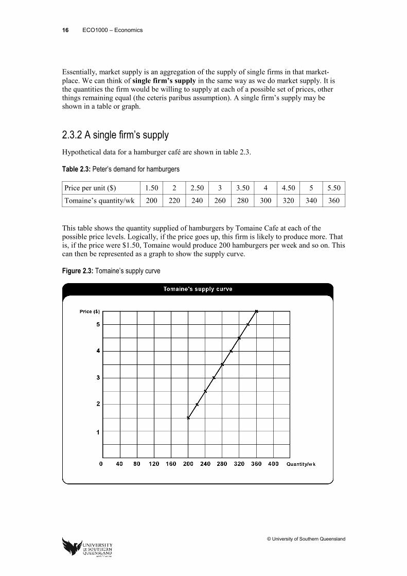
2.3.2 A single firm’s supplyHypothetical data for a hamburger café are shown in table 2.3.
Table 2.3: Peter’s demand for hamburgers
Price per unit ($) 1.50 2 2.50 3 3.50 4 4.50 5 5.50
Tomaine’s quantity/wk 200 220 240 260 280 300 320 340 360
This table shows the quantity supplied of hamburgers by Tomaine Cafe at each of the possible price levels. Logically, if the price goes up, this firm is likely to produce more. That is, if the price were $1.50, Tomaine would produce 200 hamburgers per week and so on. This can then be represented as a graph to show the supply curve.
Figure 2.3: Tomaine’s supply curve
© University of Southern Queensland
ECO1000 – Economics 17
Interactive presentation
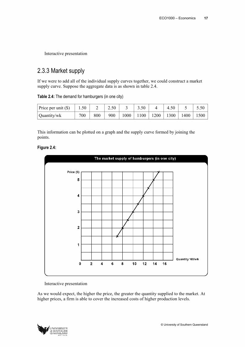
2.3.3 Market supplyIf we were to add all of the individual supply curves together, we could construct a market supply curve. Suppose the aggregate data is as shown in table 2.4.
Table 2.4: The demand for hamburgers (in one city)
Price per unit ($) 1.50 2 2.50 3 3.50 4 4.50 5 5.50
Quantity/wk 700 800 900 1000 1100 1200 1300 1400 1500
This information can be plotted on a graph and the supply curve formed by joining the points.
Figure 2.4:
Interactive presentation
As we would expect, the higher the price, the greater the quantity supplied to the market. At higher prices, a firm is able to cover the increased costs of higher production levels.
© University of Southern Queensland
18 ECO1000 – Economics
2.3.4 Movements along and shifts of the supply curveAs for the treatment of demand curves, we need to distinguish between a movement along a given supply curve and a shift of that curve. If we allow price of the good to vary, and keep all other determining economic variables constant (the ceteris paribus assumption), as price changes we move along the supply curve. This is known as a change in quantity supplied.
If we hold price constant and let any of the other determining economic variables change (such as input prices), we have a new set of price-quantity data. This change is known as a change in supply. If there is an increase in supply (more would be supplied at each and every price) the supply curve shifts to the right. If there is a decrease in supply (less would be supplied at each and every price) the supply curve shifts to the left.
2.3.5 Reasons for the supply curve to shiftAs for the treatment of demand, there are a number of ‘non-price’ determining variables of supply. When we construct the supply curve, these are held constant (the ceteris paribus assumption). If we relax that assumption and allow one of them to change, we have a change in supply (show by a shift of the curve). It is important that we can explain the effect of a change in these variables on supply. The variables include:
● prices of inputs
● technology
● prices of substitutes in production
● number of firms in the market
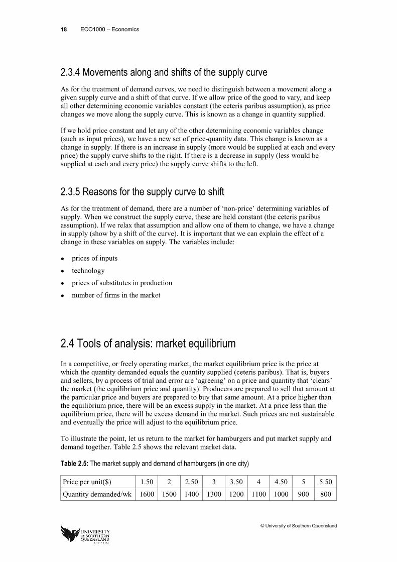
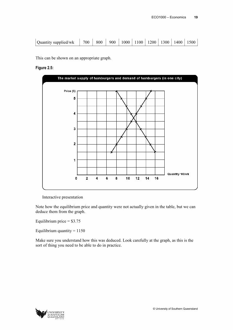
2.4 Tools of analysis: market equilibriumIn a competitive, or freely operating market, the market equilibrium price is the price at which the quantity demanded equals the quantity supplied (ceteris paribus). That is, buyers and sellers, by a process of trial and error are ‘agreeing’ on a price and quantity that ‘clears’ the market (the equilibrium price and quantity). Producers are prepared to sell that amount at the particular price and buyers are prepared to buy that same amount. At a price higher than the equilibrium price, there will be an excess supply in the market. At a price less than the equilibrium price, there will be excess demand in the market. Such prices are not sustainable and eventually the price will adjust to the equilibrium price.
To illustrate the point, let us return to the market for hamburgers and put market supply and demand together. Table 2.5 shows the relevant market data.
Table 2.5: The market supply and demand of hamburgers (in one city)
Price per unit($) 1.50 2 2.50 3 3.50 4 4.50 5 5.50
Quantity demanded/wk 1600 1500 1400 1300 1200 1100 1000 900 800
© University of Southern Queensland
ECO1000 – Economics 19
Quantity supplied/wk 700 800 900 1000 1100 1200 1300 1400 1500
This can be shown on an appropriate graph.
Figure 2.5:
Interactive presentation
Note how the equilibrium price and quantity were not actually given in the table, but we can deduce them from the graph.
Equilibrium price = $3.75
Equilibrium quantity = 1150
Make sure you understand how this was deduced. Look carefully at the graph, as this is the sort of thing you need to be able to do in practice.
© University of Southern Queensland
20 ECO1000 – Economics
Reading activity 2.1Study chapter 3 of the text (Hubbard et al.).
Make sure that you can:
● explain the ‘law of demand’
● explain why the demand curve is downward-sloping
● distinguish between a movement along and a shift of a demand curve
● explain and illustrate the effect on demand of changes in non-price determinants of demand
● illustrate the concept of demand using either a table or a demand curve.
● explain the ‘law of supply’
● distinguish between a movement along and a shift of a supply curve
● explain and illustrate the effect on supply of changes in non-price determinants of supply
● illustrate the concept of supply using either a table or a supply curve.
● explain the concepts of equilibrium price and quantity
● explain the concepts of market ‘surplus’ and market ‘shortage’
● explain and illustrate the effect of a market shortage on market price
● explain and illustrate the effect of a market surplus on market price.
Learning activity 2.1NB: This is the essential set of exercises. If you have additional time, you should practise the quizzes and tests in MyEconlab.
2.3.1 Answer Review Questions 1-10 at the end of chapter 3 (check your answers with those from the StudyDesk).
2.3.2 Answer Problems and Applications 1, 2, 3, 4, 6, 9, 10, 11, 12, 13, 14, 15, 16, 17, 18, 19, 20 at the end of chapter 3 (check your answers with those from the StudyDesk).
2.5 Elasticity
2.5.1 IntroductionIn our development of the tools of analysis above, we have used a downward-sloping demand curve and an upward-sloping supply curve. When changes in price or other economic variables occurred, we focussed on the direction of the resulting effect on prices and
© University of Southern Queensland
ECO1000 – Economics 21
quantities, rather than on the responsiveness of the dependent economic variable. If we had a measure of responsiveness of one economic variable to a change in another (for example, the responsiveness of quantity demanded to a price change), we could take out analysis to the next level and reach more useful conclusions.
Elasticity is a measure of responsiveness. In this section of the module, we introduce the concept of elasticity, study the calculation and interpretation of various elasticity measures, and see how knowledge of elasticity can be used in market analysis.
2.5.2 The concept of elasticityElasticity is a measure of responsiveness. It is a measure of the responsiveness in one economic variable (the dependent variable) to a change in another economic variable (the independent variable). For example, consider the ‘own-price’ elasticity of demand; this is a measure of the responsiveness in the quantity demanded of a good to a change in its price. Or, consider the price elasticity of supply; this is a measure of the responsiveness in quantity supplied of a good to a change in the price of the good. Clearly, the responsiveness in either case could be high or low. The measure that we calculate for the elasticity indicates to us the relative size of the responsiveness. There are many measures of elasticity that we could calculate using appropriate economic variable. Here we focus on some of the most common ones.
2.5.3 Price elasticity of demandPrice elasticity of demand is a measure of the responsiveness in quantity demanded of a good to a change in the price of that good. The calculation is straightforward, but the resultant elasticity does require correct interpretation.
2.5.4 Cross-price elasticity of demandCross-price elasticity of demand is defined as the responsiveness in the quantity demanded of a good to a change in the price of another good. The value calculated for the cross-price elasticity of demand may be positive or negative, and high or low. If the value calculated is positive, the goods are substitutes; if the value is negative, the goods are complements. Knowledge of cross-price elasticities may help in defining industries and seeing the strength of the cross-price link between goods. For example, the cross-price elasticity of demand between Toyota four-wheel drives and Mitsubishi four wheel drives would be of interest to firms producing those vehicles as they determine their pricing policy.
2.5.5 Income elasticity of demandIncome elasticity of demand is defined as the responsiveness in quantity demanded of a good to a change in money income. The value calculated for income elasticity of demand may be positive or negative, and high or low. The sign for the calculated value tells whether the good is a normal one (positive value) or an inferior one (negative value). Knowledge of
© University of Southern Queensland
22 ECO1000 – Economics
this elasticity would be of use to business and governments seeking to cater for populations with rising incomes.
2.5.6 Price elasticity of supplyThe price elasticity of supply (often just the elasticity of supply) is defined as the responsiveness in quantity supplied of a good to a change in the price of that good. This elasticity may be of high or low value, and various cases are distinguished in terms of that value. It is of interest to market analysts as they consider supply responses; for example, the change in the quantity of oil supplied to the world market as the price of oil rises.
Reading activity 2.2Study chapter 4 of the text (Hubbard et al.).
Make sure that you can:
● define and calculate ‘price elasticity of demand’
● explain the midpoint formula for the calculation of price elasticity of demand
● distinguish among elastic demand, inelastic demand and unit elastic demand
● outline the determinants of price elasticity of demand
● interpret calculated price elasticities of demand
● explain why price elasticity of demand varies along a straight line demand curve and the relationship between price elasticity and total revenue
● define ‘cross-price elasticity of demand’
● define the terms ‘complements’ and ‘substitutes’ in terms of the cross-price elasticity of demand
● interpret calculated cross-price elasticities.
● define ‘income elasticity of demand’
● define the terms ‘normal’ and ‘inferior’ goods in terms of income elasticity of demand
● interpret calculated income elasticities of demand.
● define price elasticity of supply
● understand the determinants of the price elasticity of supply
● distinguish and illustrate the various cases of elastic and inelastic supply
● interpret calculated supply elasticities.
© University of Southern Queensland
ECO1000 – Economics 23
Learning activity 2.2NB: This is the essential set of exercises. If you have additional time, you should practise the quizzes and tests in MyEconlab.
2.7.1 Answer Review Questions 1-12 for chapter 4 (check your answers with those from the StudyDesk).
2.7.2 Answer Problems and Applications 1, 2, 3, 4, 5, 6, 7, 8, 9, 10, 12, 13, 15, 17, 18, 19 for chapter 4 (check your answers with those from the StudyDesk).
2.6 Economic efficiency and market failure Now that we have developed a number of the tools used by economists, let us turn our attention to the use of those tools. In this section of the module, we explore the effects of government policy to control prices in a market, the economic impact of taxes and the interesting question of why markets may fail to provide desirable outcomes in an economy. Before we go into all these applications, we introduce the concepts of consumer and producer surplus first.
2.6.1 Consumer and producer surplus and economic efficiencyConsumer surplus is the difference between the highest price a consumer is willing and able to pay and the price the consumer actually pays.
Producer surplus is the difference between the lowest price a firm would have been willing and able to accept and the price it actually receives.
When equilibrium is reached in a competitive market, the marginal benefit from the last unit sold will equal the marginal cost of producing that last unit. This is an economically efficient outcome.
If less than the equilibrium output were produced, the marginal benefit of the last unit bought would exceed its marginal cost.
If more than equilibrium quantity were produced, the marginal benefit of this last unit would be less than its marginal (opportunity) cost.
Economic surplus is the sum of consumer and producer surplus. Economic surplus, or the net benefit to society from the production of a good or service, is maximised at equilibrium in a competitive market (when there are no externalities).
A deadweight loss is the reduction in economic surplus resulting from a market not being in competitive equilibrium.
© University of Southern Queensland
24 ECO1000 – Economics
Economic efficiency is a market outcome in which the marginal benefit to consumers of the last unit produced is equal to its marginal cost of production, and where the sum of consumer and producer surplus is at a maximum.
2.6.2 Price floors and price ceilingsThough the total benefit to society is maximised at a competitive market equilibrium, individual consumers would be better off if they could pay a lower than equilibrium price, and individual producers would be better off if they could sell at a higher than equilibrium price.Consumers and producers sometimes lobby government to legally require a market price different from the equilibrium price. These lobbying efforts are sometimes successful.
A price floor is a legally determined minimum price that sellers may receive.
Price floors were established in agricultural markets in the USA, European Union (EU) and in many other countries in response to pleas from farmers who could sell their product only at low prices.
A price ceiling is a legally determined maximum price that sellers may charge.
It is reported that Venezuelan President Hugo Chavez's policy of keeping a tight control on food retail prices have caused severe food shortage in recent years.
2.6.3 The economic impact of taxesWe are now in a position to return to market analysis and to see how knowledge of elasticity enables us to draw useful conclusions about market changes. Here we focus on the effects of a tax (such as a sales tax) imposed on the sale or the production of goods and services.
A tax on the sale of a good or service also results in a reduction of economic efficiency. For example, if the federal government were to impose an additional tax on cigarettes of $1.00 per pack, this would decrease the supply (shift the supply curve of cigarettes to the left, or shift it up by $1.00). The tax would result in a loss of consumer and producer surplus. Some of the reduction of consumer and producer surplus becomes government revenue and the rest is a deadweight loss, which is referred to as the excess burden of the tax.
The incidence of a tax is the actual division of the excess burden between producers and consumers in the market. The tax incidence varies depending on how responsive producers and consumers are to the price change caused by the tax (ie, elasticities of demand and supply).
© University of Southern Queensland
ECO1000 – Economics 25
Reading activity 2.3Study chapter 5 of the text (Hubbard et al.).
Make sure that you can:
● explain the concepts of consumer surplus and producer surplus
● explain the concepts of marginal benefit and marginal cost
● explain and illustrate the concept of economic efficiency
● explain and illustrate the effect of the policy of setting a price floor in a market
● explain and illustrate the effect of the policy of setting a price ceiling in a market.
● illustrate the effect of taxes on economic efficiency
● define the term ‘tax incidence’
● use a supply and demand diagram to illustrate the tax incidence of a unit tax (tax placed on each unit of a good) in terms of prices paid and received, and in terms of tax paid by buyers and sellers
● discuss the importance of demand and supply elasticity for the determination of the tax paid by buyers and sellers when a unit tax is imposed.
Learning activity 2.3NB: This is the essential set of exercises. If you have additional time, you should practise the quizzes and tests in MyEconlab.
2.8.1 Answer Review Question 1-12 at the end of chapter 5 (check your answers with those from the StudyDesk).
2.8.2 Answer Problems and Applications 1, 2, 3, 4, 5, 7, 8, 9, 10, 11, 14, 17, 19, 20 at the end of chapter 5 (check your answers with those from the StudyDesk).
SummaryIn this module, we introduced a number of important tools for use in economic analysis. These were the concepts of demand, supply, market equilibrium, consumer surplus, producer surplus and elasticity. Use of these concepts, often in terms of graphical analysis, enables us to work out the effects of changes in a competitive market in terms of changes in prices, quantities, and revenues. We are now able to use the economic way of thinking to analyse a wide range of market situations.
© University of Southern Queensland

26 ECO1000 – Economics
© University of Southern Queensland
ECO1000 – Economics 27
Module 3 – Firms and market structure
Learning objectivesOn successful completion of this module, you should be able to:
● explain the concepts of ‘explicit’ and implicit’ costs
● use the law of diminishing returns to explain and illustrate the short-run production function
● explain the relationship between short run costs and output in terms of total, average, and marginal cost curves
● explain the relationship between marginal and average cost and between marginal product and marginal cost
● explain the construction and shape of the firm’s long run average cost curve
● explain the model of perfect competition.
● explain the model of monopoly
● discuss the efficiency issues in both perfectly competitive market and monopoly market.
Learning resources
TextHubbard et al. 2013, Economics, chapters 6, 7 and 8.
EssentialStudy book: module 3.
3.1 IntroductionIn modules 1 and 2, we used the concepts of the production possibilities frontier, the supply curve, and market equilibrium without going into much detail about the underlying economics. In this module, we will explore the economics of production, costs and the market structures of perfect competition and monopoly.
Our earlier analysis of market equilibrium assumed a market structure of perfect competition: one in which there are many buyers and sellers and in which no individual buyer or seller has any market power over price.
© University of Southern Queensland
28 ECO1000 – Economics
In this module, we add to our study of economic models by examining the model of perfect competition. This is the well-known model of the ‘free market’; a model which lies at the heart of much of the argument about the need to make actual markets more competitive.
To understand the operation of this model, we need to consider carefully the relationships between production and cost in both the short run time period and the long-run time period. Once we know a typical firm’s short run and long run cost functions (the relationships between cost and output), we can combine this information with information about the revenue function (the relationship between output and revenue) to work out how much output a firm will be willing to supply. From this, we can deduce the shape of the market supply curve which is used in market analysis.
A monopoly is a firm that is the only seller of a good or service that does not have a close substitute. For a monopoly to exist barriers to entering the market must be so high that no other firms can enter. A monopolist will produce less and charge a higher price than would a perfectly competitive industry producing the same good. The monopolist’s profit-maximising price exceeds marginal cost. The monopoly equilibrium is neither productively efficient nor allocatively efficient.
There are a number of production, cost and revenue concepts to be understood in this module. We begin with production and costs in the two time periods and then turn to the analysis of the perfectly competitive firm and market.
3.2 The concept of cost revisitedIn module one, we introduced the concept of opportunity cost. Opportunity cost is an important consideration when business decisions are made. Most people would be familiar with the basic idea of business costs, which would include wages for workers, materials, other production costs, and capital costs for buildings and equipment. Think of these as accounting costs, or the payments for actual things; that is think of them as explicit costs. Business profit is calculated as:
Revenue (or income) – accounting costs = profit.
Audio: explicit costs explicit costs
This seems quite simple, but economists believe that such a simple calculation misleads the business person. The economic question is: what has the business owner foregone in order to be in a particular business?
Suppose that Sally earns $100 000 a year as a corporate economist, but like many people she wants to ‘be her own boss’. She buys a small business for $300 000, using funds she inherited. However, she realises the new business can only afford to pay her a managing director’s salary of $80 000. Sally is ‘paying’ an implicit cost for her decision to be an owner operator. This implicit cost is the $20 000 a year in her personal income ($100 000 – $80 000) that she foregoes.
© University of Southern Queensland
ECO1000 – Economics 29
She also foregoes interest income by investing her funds in the business, rather than in financial assets. Suppose that the current interest rate is 10%. This is taken to be the return on the best alternative use of her funds. Sally could be earning $30 000 a year from a financial investment of $300 000 at 10% per year.
In total, the annual implicit cost she incurs by investing in the business is:
$20 000 + $30 000 = $50 000 per year
This cost should be added to the explicit accounting cost to give the economic cost of choosing the business option. That is:
Economic cost = accounting cost (explicit costs) + implicit cost (implicit costs).
Audio: economic costs economic costs
Audio: implicit costs implicit costs
This does not mean that business people should slavishly follow such a principle and always pursue the alternative yielding the highest return. People go into business for all sorts of reasons, including job satisfaction, the desire for independence and to create family assets. In addition, in some years, profits will be down compared to other investments, so the opportunity cost will be higher, but you would not necessarily sell out to pursue always the short term best option. There are costs in transferring assets and skills. There may also be taxation benefits in having a business which yields a better return than salaries, although this can be overestimated. The important point to note is that as a business person, you should know what the options are and how much your choices really ‘cost’. Harsh as it may seem, if you stay in an enterprise that has a persistent negative economic profit, you might have difficulty. Over time, the temptation to pursue better options will increase.
In summary, in economics we measure costs as opportunity costs including explicit costs and implicit costs. Explicit costs are the payments to non-owners of a firm for their resources, e.g., wages, lease payments, cost of materials, etc. Implicit costs are the opportunity costs that do not require an outlay of money by the firm, e.g., the use of the owner's time, money and car for production.
© University of Southern Queensland
30 ECO1000 – Economics
3.3 The short run production functionEconomists usually consider the economics of a firm’s production in two time periods. The short run is that time period in which at least one of the firm’s inputs is fixed in quantity. The long run time period is that time period in which all of a firm’s inputs can be considered to be variable in quantity. This leads to the classification of inputs as variable or fixed, depending on the time period in question.
Given this time period distinction, we can speak of the firm’s short and long run production functions, where a production function refers to the relationship between the inputs used by a firm and the output it produces. These production functions become the basis for the firm’s cost functions in the long and short run time periods.
If we assume that labour and machine capital are the only two inputs for a firm and the number of machines is fixed. The marginal product of labour is the additional output the firm produces as a result of hiring one more worker. The law of diminishing returns states that at some point, adding more of a variable input, such as labour, to the same amount of a fixed input, such as capital, will cause the marginal product of the variable input to decline.
The average product of labour is the total output produced by a firm divided by the quantity of workers. When the average product is rising, the marginal product is above the average product; when the average product is falling, the marginal product is below the average product. Therefore, the marginal product curve cuts the average product curve at the point where the average product is at its maximum.
3.4 Short run cost functionsWith our knowledge of the short run production function, we can turn to a consideration of a firm’s short run cost function. This is the relationship between a firm’s output and costs. The cost function can be displayed in terms of its output and total costs (total fixed cost, total variable cost and total cost), or in terms of its output and its average costs (average fixed cost, average variable coast, and marginal cost). We need to understand the shape of the typical cost curves (functions) and to appreciate that there are geometrical relationships between the various cost curves that need to be observed when we draw and interpret the cost relationships.
Marginal cost is the change in a firm’s total cost from producing one more unit of a good or service. The law of diminishing returns explains why the marginal cost curve is U-shaped. The relationship between marginal cost and average total cost can be explained as: when MC is below ATC, ATC will fall; when MC is above ATC, ATC will rise; MC curve cuts ATC curve when ATC is at its lowest point; the ATC curve is U-shaped because MC is U-shaped. The same reasoning applies to the relationship between MC and AVC.
© University of Southern Queensland
ECO1000 – Economics 31
3.5 Long run average costIn the long run period, all inputs are variable. Consequently, all costs are variable as well. For this time period, economists use the concept of long run average cost to represent the long run cost function. This cost function is typically U-shaped and is formed by the lowest portions of the set of short run cost functions that enable production at least cost as output is increased. As we explore the long run cost function, we need to note that the long run is essentially a firm’s planning period. Once a decision has been made to build a certain size of plant, the firm is operating in the short run.
Reading activity 3.1Study chapter 6 of the text (Hubbard et al.).
Make sure that you can:
● understand the concepts of 'short run' and 'long run'
● define total cost, variable cost and fixed cost
● define the terms ‘explicit’ and ‘explicit cost’
● explain the concept of a ‘production function’
● calculate average cost
● explain the concepts of ‘marginal product’ and 'average product'
● state the law of diminishing returns
● explain the relationship between marginal and average product.
● define and calculate average marginal cost, fixed cost, average variable cost, and average total cost
● explain and illustrate the relationship between marginal cost and average cost
● interpret graphs showing either total cost curves, or average cost curves
● explain and illustrate a firm’s long run average cost curve in terms of a series of short average run cost curves
● explain the typical shape of the long run average cost curve in terms of ‘economies’ of scale; ‘diseconomies’ of scale and ‘constant returns’ to scale.
© University of Southern Queensland
32 ECO1000 – Economics
Learning activity 3.1NB: This is the essential set of exercises. If you have additional time, you should practise the quizzes and tests in MyEconlab.
3.4.1 Answer Review Questions 1-10 for chapter 6 (check your answers with those from the StudyDesk).
3.4.2 Answer the study questions and problems 1, 3, 4, 5, 6, 7, 8, 10, 11, 12, 13, 14, 15, 18, 20 for chapter 6 (check your answers with those from the StudyDesk).
3.6 The model of perfect competition
3.6.1 IntroductionThis is one of the most well-known models of the standard microeconomics literature. It deals with a market structure in which there are many buyers and sellers, and in which no buyer or seller has any power over the price in the market. Like all models, there are a number of assumptions made about this market structure. Given these assumptions, a number of important conclusions about firm and industry pricing and production follow. We will find that, although it might be somewhat unrealistic in terms of typical market structures in existence today, it still provides a very useful beginning to our study of the way in such competitive forces work.
In our study of this model, we will look at the firm and the market (industry) in both the short and the long run periods. We will use our knowledge of cost functions for these periods to see how firm’s decide on their choice of output, and how these choices flow into industry supply. This will complete our understanding of the economics ‘beneath’ the market supply curve that we have met already in the previous module.
3.6.2 The perfectively competitive model: in the short runIn a perfectly competitive market, each individual firm is a price taker and its demand curve is horizontal, which is different from the downward-sloping market demand curve. The individual firm cannot decide the market price, but it can decide its optimal output level based on its marginal cost information to maximise the profit.
The profit is maximised at the output where the difference between total revenue (TR) and total cost (TC) is the largest. It is equivalent to say that the profit is maximised at the level of output where the firm's marginal cost equals the market price.
The firm will make an economic profit if P > ATC. The firm will break even if P = ATC. The firm will experience a loss if P < ATC.
In the short run, the firm will stay in the business if P>AVC. The firm will shut down if P<AVC. There is no difference for the firm to shut down or to continue to operate if
© University of Southern Queensland
ECO1000 – Economics 33
P=AVC. So the firm's marginal cost curve is its supply curve only for prices at or above average variable cost. The market supply curve is the horizontal sum of the individual firms' supply curves.
3.6.3 The entry and exit of firms in the long run and efficiencies in perfect competition While entry into, and exit from, the industry is not possible in the short run (firms adjust by changing their output), in the long run firms may exit the industry and new firms may enter. If a firm cannot make a normal profit (a term that means zero economic profit or break even), it will leave the industry. If firms outside the industry observe that more than normal profits are made within it, they will seek to enter the industry. Consequently, in the long run there are both industry and firm adjustments to consider. This makes the analysis slightly more complicated.
A long-run supply curve represents the relationship between market price and the quantity supplied. Its position is determined by the minimum point of the ATC curve. In the long run, the ATC could increase, decrease or remain constant. Therefore, the long-run supply curve could be upward sloping, downward sloping or horizontal.
Perfect competition can be used as a benchmark to compare with other market structures such as monopoly. In the absence of external cost or benefits a perfectly competitive market can achieve allocative efficiency in both short run and long run as the price is equal to the marginal cost(P=MC), meaning that the scarce resources are allocated in accordance with the wishes of consumers. Productive efficiency also occurs when price equals the minimum of average total cost (P=minATC). This may not be achieved in the short run, but productive efficiency is attained in the long run in perfect competition.
Productive efficiency is the situation in which a given quantity of a good or service is produced using the least amount of inputs (P=min ATC).
Allocative efficiency is a state of the economy in which production reflects consumer preferences; in particular, every good or service is produced up to the point where the last unit produced provides a marginal benefit to consumers equal to the marginal cost of producing it (P=MC).
Dynamic efficiency is the ability for firms over time to develop and utilise technological innovation, and to adapt their product to changes in consumer preferences and tastes. However, it is debatable whether a firm in a competitive environment is more innovative or a monopoly firm tends to be more innovative.
© University of Southern Queensland
34 ECO1000 – Economics
Reading activity 3.2Study chapter 7 of the text (Hubbard et al.).
Make sure that you can:
● describe the characteristics of the market structure of perfect competition
● explain why a perfectly competitive firm is a ‘price-taker’ and that its demand curve is perfectively elastic
● explain and illustrate why a perfectly competitive firm maximises profit (or minimises losses) when marginal revenue is equal to marginal cost, or total revenue minus total cost is a maximum
● explain why a perfectly competitive firm will ‘shut down’ if the price falls below average variable cost
● explain and illustrate the construction of perfectly competitive firm’s short run supply curve
● explain and illustrate the construction of the perfectly competitive industry’s supply curve.
● explain why a perfectly competitive firm in long run equilibrium makes zero economic profit (normal profit)
● explain why a perfectly competitive industry is in long run equilibrium when each firm is producing an output for which price is equal to short run marginal cost, short run average total cost and long run average cost
● explain productive, allocative and dynamic efficiencies.
Learning activity 3.2NB: This is the essential set of exercises. If you have additional time, you should practise the quizzes and tests in MyEconlab.
3.6.1 Answer Review Questions 1-12 for chapter 7 (check your answers with those from the StudyDesk).
3.6.2 Answer Problems and Applications 1, 2, 3, 5, 6, 7, 8, 9, 10, 11, 12, 13, 14, 16, 17, 18, 19 for chapter 7 (check your answers with those from the StudyDesk).
3.7 Monopoly markets
3.7.1 Monopoly modelA monopoly is a firm that is the only seller of a good or service that does not have close substitutes. Although few firms are monopolies, the economic model of monopoly can still
© University of Southern Queensland
ECO1000 – Economics 35
be very useful. As with the perfect competition model, which provides a benchmark for how a firm acts in an industry where many firms supply identical product, monopoly provides a benchmark for the other extreme, where a firm is the only supplier and faces no competition from other firms.
There are higher barriers in the monopoly market which prevent other firms from entering. The barrier could be created by the government, for example, blocking the entry of more than one firm into a market, or because the firm controls over a material necessary to produce a product. The barriers could also result from important network externalities and economies of scale.
The monopoly firm is a price maker. But it is constrained by the downward-sloping demand curve. A monopoly firm’s demand curve is the market demand curve. A monopoly firm maximises profit by producing the level of output where marginal revenue equals marginal cost.
Please note that profit is not guaranteed in a monopoly market. If the demand is very low while the firm's ATC is very high, the firm could make a loss. However, if the monopolist’s price exceeds its average total cost at the output where marginal revenue equals marginal cost, it will earn an economic profit. Because of high entry barriers new firms will not be able to enter the market, so if other things remain the same, the firm will be able to continue to earn economic profits, even in the long run.
A monopolist will produce less and charge a higher price than would a perfectly competitive industry producing the same good. The monopolist’s profit-maximising price exceeds marginal cost (P>MC) and the firm does not produce at the minimum point of ATC (P>min ATC). Thus the monopoly equilibrium is neither productively efficient nor allocatively efficient.
3.7.2 Economic efficiency and government regulation in monopoly market Compared to equilibrium in a perfectly competitive market, which results in the maximum amount of economic surplus, a monopoly will produce less and charge a higher price, resulting in reduction in consumer surplus and allocative efficiency. This is actually another form of market failure. Therefore, government plays an important role in such markets to promote competition, thereby improving efficiency.
The Australian Competition and Consumer Commission (ACCC) monitors competitive behaviour in Australia, and enforces the Competition and Consumer Act 2010 (CCA), which contains laws against anti-competitive actions by firms.
The ACCC cracks down price-fixing activities (collusion) and regulates business mergers.
Federal, state or territory government regulatory commissions usually set prices for natural monopolies.
However, given the important role played by the application of new production methods and equipment in the productive growth of industrial countries, some economists argue that
© University of Southern Queensland
36 ECO1000 – Economics
dynamic efficiency should be given the highest priority, followed by productive efficiency. As a result, allocative efficiency is said to be of less policy importance (a normative statement!). Having done this module, students should be able to formulate their own argument on this issue.
Reading activity 3.3Study chapter 8 of the text (Hubbard et al.).
Make sure that you can:
● explain entry barriers created by government action, control of key resources, network externalities and natural monopoly
● explain and illustrate how a monopoly firm determines its output and price
● explain and illustrate consumer surplus, producer surplus and deadweight loss in a monopoly market
● Understand the concept of 'market power'
● explain why there is a need to regulate collusive behaviour and merger activities
● Understand the practices in regulating natural monopolies
Learning activity 3.3NB: This is the essential set of exercises. If you have additional time, you should practise the quizzes and tests in MyEconlab.
3.6.1 Answer Review Questions 1-12 for chapter 8 (check your answers with those from the StudyDesk).
3.6.2 Answer Problems and Applications 1, 2, 3, 4, 7, 8, 9, 10, 11, 12, 13, 14, 15, 16, 17, 19, 20 for chapter 8 (check your answers with those from the StudyDesk).
SummaryIn this module, we have explored the concepts of short and long run production and cost functions and used these in the analysis of two extreme market structures: perfect competition and monopoly. We have seen how a firm’s short run cost curves may be displayed in terms of total or average costs and that there are definite geometric relationships between the various cost curves. The long run cost curve was displayed in terms of the long run average cost curve. In the short run, the shape of the cost curves (apart from the fixed cost curve) reflects the operation of the law of diminishing returns. In the long run, it is the presence of economies and diseconomies of scale that determines the shape of the average cost curve.
© University of Southern Queensland
ECO1000 – Economics 37
Combining our knowledge of short and long run costs with the revenue function of a firm in the market structure of perfect competition, we developed the firm’s, and industry’s, short run supply curve and explored the long run adjustment of the firm and the industry. This analysis of the perfectly competitive market has given us insight into the operation of a competitive firm and the implications of this operation for the supply curve in a competitive market. This is the supply curve we used in module two when exploring market analysis in terms of demand and supply. We now know something about the economics of supply.
In a monopoly market, we have shown that deadweight loss is created as a result of higher price and lower output than those in a perfectly competitive market. Therefore, government plays an important role in safeguarding consumer welfare and promoting competition in an imperfectly competitive market.
© University of Southern Queensland

38 ECO1000 – Economics
© University of Southern Queensland
ECO1000 – Economics 39
Module 4 – Macroeconomic Foundations
Learning objectivesOn successful completion of this module, you should be able to:
● explain how total production in an economy is measured
● discuss problems encountered in the measurement of economic activity
● calculate nominal and real values of selected economic variables
● understand how the economic growth rate is measured
● discuss the importance of long-run economic growth and its impact on living standards
● define and calculate the unemployment rate and the labour fore participation rate
● explain the economic costs of unemployment
● identify the types of unemployment and explain what factors determine the natural rate of unemployment
● define the price level and the inflation rate, and understand how they are calculated
● discuss the measurement and causes of inflation.
● Understand the difference between demand-pull and cost-push
● understand what happens during business cycles and their relationship to long-run economic growth
● discuss the determinants of aggregate demand and aggregate supply.
● use the aggregate demand and aggregate supply mode to illustrate the difference between short-run and long-run macroeconomic equilibrium
● use the dynamic aggregate demand and aggregate supply model to analyse macroeconomic conditions
Learning resources
TextHubbard et al. 2013, Economics, chapters 9, 10 and 11.
EssentialStudy book: module 4.
© University of Southern Queensland
40 ECO1000 – Economics
4.1 IntroductionIn this module, we swing our attention to the economy as a whole. In the previous modules, we considered the activities of single markets that exist within a much larger set of markets and associated economic activity. This is something like flying over a forest and looking at its wide extent, rather than being inside the forest and looking at the individual trees. Now we are concerned with the overall size of the forest and at the rate at which it is changing in size. However, we will speak of the rate of economic activity, and the rate of growth of that activity, rather than size and growth of a forest.
This field of economics is often called macroeconomics, to distinguish it from the field known as microeconomics which deals with specific product, service or factor markets. We need to be aware, however, that this distinction is a modern one, and that the two fields of economics are really different ways of considering the same economy. It does not do to put these fields into separate, never to be linked, compartments. After all, the forest is made up of separate trees, and the separate trees are parts of a much larger whole.
In dealing with the economy as a whole, we have to think about the totality of economic activity and to develop ways of making sense of it. It is a rather sobering to be reminded that prior to the 1930s there were few measurements available of the size of an economy. It is only since then, and after the pioneering work of John Maynard Keynes (The General Theory of Employment, Interest and Money 1937) that more refined tools of economic analysis were available. Today, we speak of GDP and rates of growth of GDP with almost no appreciation of what these terms really mean and what pitfalls await the unwary as they use them very casually. Perhaps the protestors against globalisation have a point: what is the purpose of trying to grow as fast as possible in terms of GDP growth? Is the measure, and the underlying concept of macroeconomic activity, valid?
We turn to an examination of key macroeconomic performance data and its potential use for the design of macroeconomic policy in this module.
4.2 GDP measures total production
4.2.1 Measuring the size of the total productionFollowing the experience of the Great depression of the 1930s, when world economic activity fell to very low levels and high levels of unemployment were widespread, the need for macroeconomic data was obvious. This ushered in the development of national accounting systems; systems which enabled the consistent measurement of macroeconomic variables, such as Gross Domestic Product (GDP). It was thought that if reliable measures of the size and growth of the economic activity were available, policy-makers would be able to ensure that another great depression did not occur. Data available today for many countries is the result of the theoretical and statistical work in the field of macroeconomics. While there has not been another great depression, there has been much debate on the question of the appropriate measurement of economic activity. As a result, we are in a much better position today in our endeavour to ‘take the pulse’ of the economy.
© University of Southern Queensland
ECO1000 – Economics 41
In this section of the module, we consider the components and the measurement of GDP. These are important building blocks for our later work in which we seek to explain how the size of the circular flow changes over time.
4.2.2 The circular flow model of an economyEarly economists talked about the idea of a ‘wheel of circulation’. Perhaps they had in mind something like the great rotations of the planets, as did early viewers of the cosmos. Latter-day economists have fashioned this idea into that of the circular flow of economic activity. It is an intuitively appealing idea for we all have some appreciation of it. We know that income is earned in various ways in various activities, and that income is spent in turn on a range of goods and services, themselves the output of countless other economic activities. So, it makes some sense to us to speak of a circular flow of activity within an economy with easily recognised boundaries. We can sit back, close our eyes, and think of all the many activities that go to make up the finished goods and services and make them available to final purchasers. It is a very complex mosaic; but the idea of the circular flow helps to make sense of the overall activity that goes on every hour in any economy.
The circular flow is usually represented by a simple diagram that shows the major, aggregate flows in an economy. These diagrams can be made very complex; but that might defeat the purpose of the exercise. Our aim is to develop a workable understanding so that we can measure the size of the flow and its rate of growth. We note that underlying this idea of the flow lies that of the economy as a system. That is, of something that is characterised by input-output relations. This is very convenient for mathematicians and modellers, and has much to offer us. However, we must ask at some stage about the validity of the mathematical analogy. We might note that implied recognition of the environment as a ‘sink’, into which waste is channelled, maintains this essential ‘input-output’ conception of overall economic activity.
Therefore, when we measure the value of total production in the economy by calculating GDP, we are simultaneously measuring the value of total income. GDP is the market value of all final goods and services produced in an economy during a period of time. There are three methods to calculate GDP: the production method, the expenditure method and the income method. In this course, we place the emphasis on the expenditure method. There are four major categories of expenditures: consumption, investment, government purchases, and net exports.
GDP is not a perfect measure of total production, nor a perfect measure of wellbeing. Household production and the black economy are excluded from GDP. The GDP measure does not give us the information of the distribution of the income and output among the population. The value of leisure is not included in GDP. It does not contain the information about the level and quality of health care and education. Finally, GDP is not adjusted for pollution or other negative effects of production, changes in crime and other social problem.
Nominal GDP grows over time not only as result of increases in output but also as a result of general price rises. Changes in nominal GDP that result from price changes do not tell us anything about the performance of the economy in producing goods and services. To get a clearer picture of how much an economy is growing over time, it is necessary to adjust nominal GDP so that it reflects only changes in output and not changes in prices. This adjusted GDP allows meaningful comparisons of aggregate economic activity over time when prices are changing and is referred to as real GDP. Real GDP is the value of all final
© University of Southern Queensland
42 ECO1000 – Economics
goods and services produced during a given period based on the prices existing in a selected reference year.
4.2.3 Economic growthLong-run economic growth is the key to rising living standards. The issues of growth rates and living standards are of considerable importance in the contemporary world. With much of the world’s population in relative, if not absolute, poverty the need to understand the causes of economic growth, and to implement effective growth policy, is urgent.
Many economists have turned their attention to the causes of economic growth. One of the most well-known models of economic growth is the ‘Solow’ model, developed by Robert Solow. This model focuses upon the roles of expenditure, saving, the capital stock and technological change in the determination of an economy’s rate of economic growth. In this section of the module, we explore the main causes of economic growth and consider their implications for economic policy to promote economic growth.
Increases in real GDP per capita depend on increases in labour productivity. Labour productivity is the quantity of goods and services that can be produced by one worker or by one hour of work. Two key factors determine labour productivity: the quantity of capital per hour worked and the level of technology. Therefore, economic growth occurs if the quantity of capital per hour worked increases and if technological change occurs.
One important concept here is potential GDP, which is the level of GDP attained when all firms are producing at maximum capacity. We will frequently use this concept in the following chapters when we study macroeconomics.
Reading activity 4.1Study chapter 9 of the text (Hubbard et al.).
Make sure that you can:
● define the term ‘GDP’,
● understand the three methods of measuring GDP
● understand the four components of GDP in the expenditure method
● discuss limitations of GDP as a measure of total production and a measure of wellbeing
● calculate nominal GDP to real GDP
● calculate the economic growth
● calculate the GDP deflator
● explain the determinants of the rate of long-run growth
● use the economic growth model to explain why economic growth rates differ between countries.
© University of Southern Queensland
ECO1000 – Economics 43
Learning activity 4.1NB: This is the essential set of exercises. If you have additional time, you should practise the quizzes and tests in MyEconlab.
4.1.1 Answer Review Questions 1–12 for chapter 9 (check your answers with those from the StudyDesk).
4.1.2 Answer Problems and Applications 2, 3, 4, 5, 6, 7, 8, 9, 11, 13, 14, 17, 18, 19, 20 for chapter 9 (check your answers with those from the StudyDesk).
4.3 Unemployment and inflation
4.3.1 UnemploymentAs most people earn their livelihoods from employment, the rate of unemployment in an economy is of considerable interest to citizens and economists alike. Many people remember the economic depression of the 1930s when there was large scale unemployment across the world. The suffering and poverty that resulted sparked the desire to attempt to manage economies so that the rate of unemployment remained at acceptable levels. Success has been elusive and, at the start of the 21st century, governments still tussle with the policy mix that will provide desired rates of unemployment. In this section of the module, we consider the concept and measurement of unemployment, and the classification of unemployment by economists.
We have strict definitions for employed and unemployed for statistical purpose. People are considered employed if they worked for at least one hour in paid employment in the week before the survey. Only those who have actively looked for work in the previous four weeks and are available to work are classified as ‘unemployed’. Discouraged workers are defined as people who are available for work but have given up looking for a job during the previous four weeks because they believe no jobs are available for them. The labour force is the sum of the employed and employed. Discouraged workers are measured as ‘not in the labour force’.
There are several types of unemployment: cyclical unemployment, frictional unemployment and structural unemployment. Structural unemployment is long-term unemployment and possibly even permanent unemployment because workers need time to learn new skills and some may never learn these. The government should indeed be concerned about it since such unemployment can lead to permanent unemployment. On the other hand, cyclical unemployment is caused by lack of jobs during a recession.
Full employment occurs when the unemployment rate is equal to the total of the frictional and structural unemployment rates. Full employment, therefore, defines the rate of unemployment that exists without cyclical unemployment. The full employment rate of unemployment is also referred to as the ‘natural rate of unemployment’.
© University of Southern Queensland
44 ECO1000 – Economics
4.3.2 InflationWe are all aware that the overall price level in an economy changes from time to time, usually in an upward direction (although declines are possible). We recognise this when we speak of the rate of inflation: an inflation rate of 5% means that the overall, or general, level of prices is rising at 5%. Economists have been interested for a long time in the development of measures of the change in the overall price level. Today, such changes are measured using a price index (several indices are usually published by a country’s statistics bureau).
The most familiar price index (in Australia and many other countries) is known as the Consumer Price Index (CPI). However, CPI has some biases as a measure of inflation, which include substitution bias, increase in quality bias, new product bias and outlet bias.
Anticipated inflation does not reduce the affordability of goods and services to the average consumer, but it still imposes costs on the economy. When inflation is anticipated, its main costs are that paper money loses some of its value and firms incur menu costs. Menu costs are the costs to firms of changing prices on products and printing new catalogues. By contrast, when inflation is unanticipated, the actual inflation rate can turn out to be different from the expected inflation rate. As a result, some people gain and some people lose. Inflation affects the distribution of income, as some people will find their purchasing power is rising while other people will find their purchasing power is falling.
Inflation can be caused either by an increase in aggregate demand or by a decrease in aggregate supply. In Chapter 11, we will use the AD-AS model to illustrate demand-pull inflation and cost-push inflation.
Reading activity 4.2Study chapter 10 of the text (Hubbard et al.).
Make sure that you can:
● define the terms: ‘unemployment rate’, ‘labour force’; ‘discouraged worker’, and 'labour force participation rate'.
● discuss limitations of the unemployment rate as a measure of economic performance
● discuss the costs of unemployment
● distinguish among the four types of unemployment identified by economists
● discuss the concept of ‘full employment’
● explain what factors determine the natural rate of unemployment
● define the term: ‘inflation’
● explain how inflation is calculated using a consumer price index
● discuss limitations of using a consumer price index to measure inflation
● use price indexes to adjust for the effects of inflation
● discuss the costs of inflation to the economy
● outline the cause of inflation in terms of ‘demand pull’ and ‘cost-push’ theories of inflation.
© University of Southern Queensland
ECO1000 – Economics 45
Learning activity 4.2NB: This is the essential set of exercises. If you have additional time, you should practise the quizzes and tests in MyEconlab.
4.4.1 Answer Review Questions 1-14 for chapter 10 (check your answers with those from the StudyDesk).
4.4.2 Answer Problems and Applications 1, 2, 3, 4, 5, 6, 7, 8, 10, 12, 13, 14, 17, 18, 19, 20 for chapter 10 (check your answers with those from the StudyDesk).
4.4 The business cycleEconomists refer to the concept of the business cycle when observing the short run performance of an economy. Research has shown that, typically, the economy traces out a cyclical path of peaks and troughs separated by recession and expansion periods. Knowledge of the economy’s position in the cycle is important for the design of macroeconomic policy to ‘smooth’ the cycle.
4.5 Aggregate demand and aggregate supplyIn this section we build a macroeconomic model of the economy which may be used for macroeconomic analysis. The purpose of such analysis is to explain the current performance of the economy and to work through the effects on macroeconomic performance of possible policy changes.
We begin with some reflections on the 1930s depression and the radical work of Keynes; Keynes suggested the policy-makers should focus on aggregate demand in the economy if they wished to ‘manage’ the business cycle. We then move from the early Keynes’ model to a more recent aggregate demand (AD) and aggregate supply (AS) model which captures some of Keynes’ insights as well as those of other noted macroeconomists. This model provides quite a powerful tool for macroeconomic analysis.
Three theories can be used to explain why the AD curve is downward sloping: the wealth effect, the interest-rate effect and the international-trade effect.
We need to pay special attention to the variables that shift the AD curve: changes in government policies, changes in the expectations of households and firms and changes in foreign variables.
If there is an increase in resources such as workers, new mineral discoveries, quantity of capital and advance in new technology, the long-run AS will increase, shifting to the right. These factors also increases short-run AS. Other variables that can shift SRAS include
© University of Southern Queensland
46 ECO1000 – Economics
expected changes in the future price level, adjustments of workers and firms to errors in past expectations about the price level, and unexpected changes in the price of an important natural resource.
The LRAS is vertical while the SRAS is upward sloping because the wages and prices are 'sticky' in the short run.
The AD-AS model can be used to illustrate the effects of an decrease/increase in AD/AS on the price level and real GDP.
Reading activity 4.3Study chapter 11 of the text (Hubbard et al.).
Make sure that you can:
● define the terms: ‘peak’, ‘recession’, ‘trough’, ‘expansion’
● explain what happens during a business cycle
● explain why the aggregate demand curve downward slopping
● discuss the variables that shift the aggregate demand curve
● discuss and illustrate the shapes of the long-run and short-run aggregate supply curves
● discuss the factors that shift long-run and short-run aggregate supply curves
● understand why some firms and workers fail to predict accurately changes in the price level.
● illustrate the difference between long-run and short-run macroeconomic equilibrium using AD-AS model
● use AS-AS model to illustrate recession, expansion and supply shock
● use the dynamic AD-AS model to analyse macroeconomic conditions
Learning activity 4.3NB: This is the essential set of exercises. If you have additional time, you should practise the quizzes and tests in MyEconlab.
4.3.1 Answer Review Questions 1-14 for chapter 11 (check your answers with those from the StudyDesk).
4.3.2 Answer Problem and Applications 1, 2, 3, 4, 5, 7, 8, 11, 12, 13, 14, 15, 16, 17, 18, 19, 20 for chapter 11 (check your answers with those from the StudyDesk).
Summary
© University of Southern Queensland
ECO1000 – Economics 47
In this module, we have explored the circular flow model of the macroeconomy and used it to consider how economic activity might be measured. Any description or analysis of an economy relies upon a concept of the economy and on measurement of the economy’s rate of economic activity. The circular flow model provides one way of thinking about the activity that goes on in an economy. It also provides suggestions as to how the flow of economic activity could be measured. The concept of GDP (and related concepts) enables us to measure changes in economic activity over time, to make comparisons among countries and to explore the outcomes of policies designed to affect the rate of economic performance. While suggestions for improved concepts are often discussed, the framework for national accounting that is currently used provides a consistent method of measuring economic activity.
Production, productivity of inputs, and economic growth are very important topics in the discipline of economics and for the people of the world. Discussion about economic growth involves issues such as the rate and type of growth that is desired, ways to achieve that growth, and economic performance over a relatively long period of time. Living standards are dependent on the rate of and type of growth. Consequently, it is important that there be careful analysis of the causes of growth and of policy to promote growth.
The AD-AS model enables us to work out the effects on the price level and GDP of changes that affect either or both of the AD and AS curves. The AD curve shows the relationship between the price level and the quantity of real GDP demanded by households, firms and the government, while the short-run AS shows the relationship between the price level and the quantity of real GDP supplied by firms. The long-run AS is vertical as in the long run, real GDP is always at its potential level and is unaffected by the price level. The short-run aggregate supply curve is upward sloping because the workers and firms fail to predict accurately the future price level.
Unemployment remains a very important issue in most economies, though in some instances it appears to be surprisingly low in the order of policy objectives. Despite advances in economic understanding over the last century, there is considerable controversy over the policy a government should pursue to achieve ‘full’ employment.
Because of the existence of inflation (and sometimes deflation), it is necessary to distinguish nominal and real values of economic variables, such as GDP. Price indices, such as the CPI, are used for this purpose. These are constructed to show changes in the general price level from one period to another.
© University of Southern Queensland

48 ECO1000 – Economics
© University of Southern Queensland
ECO1000 – Economics 49
Module 5 – Monetary and Fiscal policy
Learning objectivesOn successful completion of this module, you should be able to:
● understand the definition of money and its functions
● understand the definitions of money supply
● explain how financial institutions create money
● describe the Australian financial system as an example of a typical financial system in the 21st century
● explain monetary policy and the main goal of monetary policy in Australia
● discuss how the Reserve Bank of Australia influences interest rates
● explain fiscal policy and how the government can use it to stabilise the economy
● explain the multiplier process
● understand ‘automatic stabilisers’.
● demonstrate the effects of monetary and fiscal policy using the dynamic AD-AS model
Learning resources
TextHubbard et al. 2013, Economics, chapters 12, 13 and 14.
EssentialStudy book: module 5.
© University of Southern Queensland
50 ECO1000 – Economics
5.1 IntroductionThe study of macroeconomic policy can be a frustrating experience for students. It takes some time to understand the concepts because the operations of the economy are not easily observed and understood. At least with microeconomics, students can relate the relevant concepts to specific markets they are familiar with, such as the market for CDs, or the particular labour market in which they operate. In addition, there is considerable disagreement about how an economy works, let alone how it should be managed, or even if it should be managed. Third, the relationships within the economy are highly interconnected, so that whenever one variable is changed to try and achieve a positive outcome there are many potential side-effects, some of which in turn, have negative consequences for the economy. Finally, macroeconomic policy, and the politics associated with it, seems to be far removed from the lives of students and working folk. However, while micro economic factors seem to have the most immediate effects on our lives, in relation to the cost of living and our incomes, macroeconomic factors can have a great impact on us.
Governments of differing persuasions and in different time periods try to achieve different things but, in liberal democratic countries, there are some generally agreed policy goals. These include:
● keeping inflation down
● keeping the growth rate up
● keeping unemployment down
● keeping the economy stable, so growth is relatively steady, rather than fluctuating wildly
● encouraging an increase in net exports (exports – imports).
In addition to all that, some governments also want to:
● assist the disadvantaged or, in some cases, to try and ensure a more equal distribution of income and/or wealth
● maximise economic freedom within the economy (a political principle)
● provide opportunities for people to participate in the market economy.
As might be observed, many of these goals are potentially contradictory, and the pursuit of one can compromise another.
In this module, we focus on the main types of macroeconomic policy: monetary and fiscal policy. Although we will treat them separately, we need to note that they both operate at the same time, although with different emphases. We need to note, also, that there is considerable debate among economists about how the macroeconomy works and what are the best policy settings for the purpose of achieving the policy goals.
© University of Southern Queensland
ECO1000 – Economics 51
5.2 Money, banks and the Reserve Bank of AustralianIn modern economies, the financial sector, and the financial markets associated with it, provides an essential institutional structure for the operation of the economy. The financial sector includes the banking system, a number of financial markets (such as the money market and the stock market), and a set of policy institutions (such as the central bank). It is necessary that we have a sound understanding of the nature and operation of the financial sector for our study of macroeconomic policy.
Money is any asset that people are generally willing to accept in exchange for goods and services or for payment of debts. Whether an asset can be used as money depends on whether it can fulfil the following 4 functions: medium of exchange, unit of account, store of value, standard of deferred payment.
Economists have developed several different definitions of the money supply. The narrowest definition of the money supply is M1, which includes currency in circulation and demand account balances. A broader definition of the money supply is M3, which includes M1, plus all other deposits with domestic and foreign-owned banks operating in Australia, including certificates of deposit, term deposits, and deposits with banks from building societies, credit unions and other authorised deposit-taking institutions. Broad money is the widest measure of Australia's money supply, and includes M3 plus deposits into non-bank deposit-taking financial institutions less holdings of currency and deposits of non-bank depository corporations such as finance companies, money market corporations and cash management funds.
A bank balance sheet lists a firm’s assets on the left and its liabilities and stockholders’ equity on the right. Reserves and loans are assets and deposits are liabilities. When a commercial bank receives a deposit, it keeps a part of the funds (say, 10% which is called reserve ratio determined by the central bank) as reserves and loans out the remainder. When the loan borrower buys something with the loan, the seller will deposit the payment in a bank. The seller's bank will keep a fraction of the deposit (say 10%) as reserves and loan out the remainder. The process will continue until no banks have excess reserves. In this way, the volume of deposits is created and according to the definitions of money discussed above, money supply increases.
The financial system facilitates the flow of funds from savers to borrowers. The Reserve Bank of Australia (RBA) is the central bank of Australia. Its main roles are to maintain the integrity and stability of the financial system and to manage and implement monetary policy. The RBA influences financial liquidity and interest rates through the use of open market operations.
© University of Southern Queensland
52 ECO1000 – Economics
Reading activity 5.1Study chapter 12 of the text (Hubbard et al.).
Make sure that you can:
● define money and discuss its functions.
● discuss the definitions of the money supply
● explain how financial institutions create money
● understand the role of the RBA
● explain the terms ‘simple deposit multiplier’, ‘cash rate’, and ‘open market operations’.
Learning activity 5.1NB: This is the essential set of exercises. If you have additional time, you should practise the quizzes and tests in MyEconlab.
5.1.1 Answer Review Questions 1-10 for chapter 12 (check your answers with those from the StudyDesk).
5.1.2 Answer Problems and Applications 1, 2, 4, 5, 8, 9, 10, 11, 14, 15, 17, 18, 19, 20 for chapter 12 (check your answers with those from the StudyDesk).
5.3 Monetary policyAs noted earlier, monetary policy is implemented by a country’s central bank and is concerned with the availability and price of money. The major objective of monetary policy in many countries is now seen to be the control of inflation. The actual implementation of monetary policy is a complex process, involving the monetary transmission mechanism in a country, appropriate policy choices by the monetary authorities, and the actions and reactions of consumers and firms to announced policy changes. In this section of the module, we will examine a number of key aspects of monetary policy.
The RBA is responsible for carrying out monetary policy, which in Australia refers to the actions taken by the Reserve Bank of Australia (RBA) to affect interest rates to enable it to target the rate of inflation. The RBA and the federal government have agreed that the RBA will target an inflation rate in the range of 2-3% per annum on average over the business cycle.
Money demand curve is downward sloping. When the interest rates fall, households and firms switch from holding interest-bearing financial assets to holding money. The interest rate is the opportunity cost of holding money. When the interest rates are high, firms and
© University of Southern Queensland
ECO1000 – Economics 53
households will lose if they hold too much money. Therefore, they will reduce the amount of money and switch to financial assets.
Factors that can cause the money demand curve to shift are real GDP and the price level. An increase in real GDP and price level will shift the money demand curve to the right.
It was believed that the central bank could be able to control the supply and availability of money. However, these days, the money supply has become increasingly difficult to target due to financial innovation, the huge growth of credit and the growth of the private sector's ability to affect the money supply via private bonds, securities and loans. Therefore, today the RBA has given up targeting money supply and interest rate targeting is now used. The RBA sets the cash rate on overnight loans in the money market. Other interest rates in the economy are influenced by the cash rate (usually move in the same direction). Changes in interest rates affect aggregate demand through influencing consumption, investment and net exports.
The AD-AS model can be used to demonstrate the effect of expansionary/contractionary monetary policy on the price level and real GDP. An expansionary monetary policy lowers interest rates to increase C, I and NX. This causes a rightward shift of the AD curve, leading to a higher level of price (inflation rate) and real GDP. A contractionary monetary policy works in the opposite direction.
Reading activity 5.2Study chapter 13 of the text (Hubbard et al.).
Make sure that you can:
● state the goals of monetary policy
● describe how the Reserve Bank of Australia affects interest rates
● understand the difference between nominal and real rates
● use AS-AS model to show the effects of monetary policy on real GDP and the price level.
● understand the arguments for and against the independence of the Reserve Bank of Australia.
Learning activity 5.2NB: This is the essential set of exercises. If you have additional time, you should practise the quizzes and tests in MyEconlab.
5.2.1 Answer Review Questions 1-10 for chapter 13 (check your answers with those from the StudyDesk).
5.2.2 Answer Problems and Applications 1–10, 12-20 for chapter 13 (check your answers with those from the StudyDesk).
© University of Southern Queensland
54 ECO1000 – Economics
5.4 Fiscal policyThe other major type of macroeconomic policy is fiscal policy. This is the responsibility of the Treasury in most countries and is most readily seen in the design and implementation of annual budgets.
Following the work of Keynes, for some time it was thought that governments could use fiscal policy to maintain their employment, growth and price stability objectives. This was especially so in the period immediately after the Second World War (post 1945 period). However, subsequent economic experience showed that fiscal policy may not be as useful as originally thought for economic management. Today, many commentators see economic virtue in a surplus budget. Here, we will examine the nature, implementation and possible effectiveness of fiscal policy.
Discretionary fiscal policy stems from Keynes’ argument that a government could increase aggregate demand in times of recession to stabilise the economy at a desirable level of economic activity. This would involve the government running a deficit budget (spending more than it received in revenues). Conversely, it could dampen an ‘overheated’ economy by reducing aggregate demand by running a budget surplus. In an attempt to develop successful fiscal policy, economists have explored the economic impacts of deficit and surplus budgets, the role of expenditure multipliers, and the reliance on automatic stabilisers.
Expansionary fiscal policy involves increasing government purchases or decreasing taxes, while contractionary fiscal policy involves decreasing government purchases or increasing taxes. The AD-AS model can be used to demonstrate the effects of the fiscal policy on price level and real GDP.
The multiplier effect amplifies the effect of an increase/decrease in government purchases or a cut/rise in taxes. The government purchases multiplier is the change in equilibrium real GDP divided by the change in government purchases. The tax multiplier is the change in equilibrium real GDP divided by the change in taxes. The larger the Marginal Propensity to Consume (MPC), the larger the multiplier.
However, the multiplier effect might be offset by the crowding out effect. Since the government competes with other borrower for available savings, interest rates experience upward pressure as the government seeks to borrow funds from the financial markets. The result of this rise in interest rates may be lower consumption and business investment, which would act to offset the boost in AD from the increased government spending.
The government may go into budget deficit during economic downturn and into budget surplus during economic expansion without taking any action because of the effects of automatic stabilisers. The former is caused by a drop in government tax revenue (eg, fewer wages and profits mean fewer tax revenues for the government) and an increase in transfer payments (eg, more people lose jobs and apply for unemployment benefits). The latter is caused by an increase in tax revenue and a decrease in transfer payments due to the economic expansion.
Some fiscal policies have long-run effects by expanding the productive capacity of the economy and increasing the rate of economic growth. These policies can shift the long-run AS curve to the right.
© University of Southern Queensland
ECO1000 – Economics 55
Reading activity 5.3Study chapter 14 of the text (Hubbard et al.).
Make sure that you can:
● define the term ‘discretionary fiscal policy’
● distinguish between expansionary and contractionary fiscal policies
● explain the role of the ‘multiplier’ in fiscal policy
● explain the role played by ‘automatic stabilisers’ in fiscal policy
● discuss the long-run effects of fiscal policy
Learning activity 5.3NB: This is the essential set of exercises. If you have additional time, you should practise the quizzes and tests in MyEconlab.
5.3.1 Answer Review Questions 1–10 for chapter 14 (check your answers with those from the StudyDesk).
5.3.2 Answer Problems and Applications 1–20 for chapter 14 (check your answers with those from the StudyDesk).
SummaryIn this module, we have explored the important area of macroeconomic policy. Our focus was on monetary and fiscal policy and the use of macroeconomic theory to explain policy choice and to predict the macroeconomic effects of that choice. Designing and implementing macroeconomic policy is a complex task. We should now be in a position to use available data and policy information to explain and critique contemporary macroeconomic policy. Tables 5.1 and 5.2 summarise the consequences of policy and monetary policy (some points are not covered by our text, so just for your interest) which can help you to better understand the content of this module.
© University of Southern Queensland
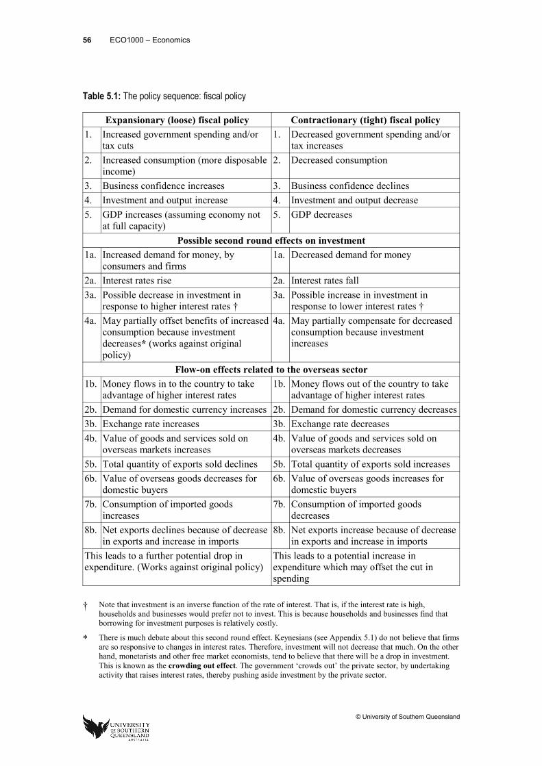
56 ECO1000 – Economics
Table 5.1: The policy sequence: fiscal policy
Expansionary (loose) fiscal policy Contractionary (tight) fiscal policy1. Increased government spending and/or
tax cuts1. Decreased government spending and/or
tax increases2. Increased consumption (more disposable
income)2. Decreased consumption
3. Business confidence increases 3. Business confidence declines4. Investment and output increase 4. Investment and output decrease5. GDP increases (assuming economy not
at full capacity)5. GDP decreases
Possible second round effects on investment1a. Increased demand for money, by
consumers and firms1a. Decreased demand for money
2a. Interest rates rise 2a. Interest rates fall3a. Possible decrease in investment in
response to higher interest rates †3a. Possible increase in investment in
response to lower interest rates †4a. May partially offset benefits of increased
consumption because investment decreases* (works against original policy)
4a. May partially compensate for decreased consumption because investment increases
Flow-on effects related to the overseas sector1b. Money flows in to the country to take
advantage of higher interest rates1b. Money flows out of the country to take
advantage of higher interest rates2b. Demand for domestic currency increases 2b. Demand for domestic currency decreases3b. Exchange rate increases 3b. Exchange rate decreases4b. Value of goods and services sold on
overseas markets increases4b. Value of goods and services sold on
overseas markets decreases5b. Total quantity of exports sold declines 5b. Total quantity of exports sold increases6b. Value of overseas goods decreases for
domestic buyers6b. Value of overseas goods increases for
domestic buyers7b. Consumption of imported goods
increases7b. Consumption of imported goods
decreases8b. Net exports declines because of decrease
in exports and increase in imports8b. Net exports increase because of decrease
in exports and increase in importsThis leads to a further potential drop in expenditure. (Works against original policy)
This leads to a potential increase in expenditure which may offset the cut in spending
† Note that investment is an inverse function of the rate of interest. That is, if the interest rate is high, households and businesses would prefer not to invest. This is because households and businesses find that borrowing for investment purposes is relatively costly.
* There is much debate about this second round effect. Keynesians (see Appendix 5.1) do not believe that firms are so responsive to changes in interest rates. Therefore, investment will not decrease that much. On the other hand, monetarists and other free market economists, tend to believe that there will be a drop in investment. This is known as the crowding out effect. The government ‘crowds out’ the private sector, by undertaking activity that raises interest rates, thereby pushing aside investment by the private sector.
© University of Southern Queensland
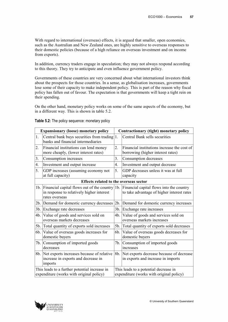
ECO1000 – Economics 57
With regard to international (overseas) effects, it is argued that smaller, open economies, such as the Australian and New Zealand ones, are highly sensitive to overseas responses to their domestic policies (because of a high reliance on overseas investment and on income from exports).
In addition, currency traders engage in speculation; they may not always respond according to this theory. They try to anticipate and even influence government policy.
Governments of these countries are very concerned about what international investors think about the prospects for those countries. In a sense, as globalisation increases, governments lose some of their capacity to make independent policy. This is part of the reason why fiscal policy has fallen out of favour. The expectation is that governments will keep a tight rein on their spending.
On the other hand, monetary policy works on some of the same aspects of the economy, but in a different way. This is shown in table 5.2.
Table 5.2: The policy sequence: monetary policy
Expansionary (loose) monetary policy Contractionary (tight) monetary policy1. Central bank buys securities from trading
banks and financial intermediaries1. Central Bank sells securities
2. Financial institutions can lend money more cheaply, (lower interest rates)
2. Financial institutions increase the cost of borrowing (higher interest rates)
3. Consumption increases 3. Consumption decreases4. Investment and output increase 4. Investment and output decrease5. GDP increases (assuming economy not
at full capacity)5. GDP decreases unless it was at full
capacityEffects related to the overseas sector
1b. Financial capital flows out of the country in response to relatively higher interest rates overseas
1b. Financial capital flows into the country to take advantage of higher interest rates
2b. Demand for domestic currency decreases 2b. Demand for domestic currency increases3b. Exchange rate decreases 3b. Exchange rate increases4b. Value of goods and services sold on
overseas markets decreases4b. Value of goods and services sold on
overseas markets increases5b. Total quantity of exports sold increases 5b. Total quantity of exports sold decreases6b. Value of overseas goods increases for
domestic buyers6b. Value of overseas goods decreases for
domestic buyers7b. Consumption of imported goods
decreases7b. Consumption of imported goods
increases8b. Net exports increases because of relative
increase in exports and decrease in imports
8b. Net exports decrease because of decrease in exports and increase in imports
This leads to a further potential increase in expenditure (works with original policy)
This leads to a potential decrease in expenditure (works with original policy)
© University of Southern Queensland
58 ECO1000 – Economics
You can see from this how governments must try to anticipate the possible outcomes. There are many variables, and responses will often depend on the situation.
In general, the theory and recent practice favours monetary policy. However, there are political pressures for governments to spend money, though not always just to influence the state of the economy. Tax cuts are thought to be a popular policy, so there is always pressure for some stimulation.
© University of Southern Queensland
ECO1000 – Economics 59
Appendix 5.1 (optional reading, and not examinable)
Epilogue: brief review of selected schools of thought in economicsIt has become apparent as we have progressed through the course that economists disagree about both theory and policy prescriptions. Essentially, it is argued that they disagree because:
● at the most fundamental level, they disagree about the assumptions in economic models, including what motivates people and how economies work. In other words, they disagree about what is really going on and, if you start with a different set of assumptions, then you are bound to finish with different conclusions about what ‘should be done’
● like all of us, economists’ views of the world and advocacy for certain courses of action are influenced by their fundamental values. For example, someone who strongly believes in economic equity is going to have greater reservations about a market system, than someone who strongly believes in the principle of individual freedom.
Much of this course has been taught as if there is not too much disagreement about economic theories and it is fair to say that much of what has been taught is considered mainstream economics. However, the reason for having limited discussion of the key debates in economics is not so much a commitment to the mainstream, as a problem of time and teaching restrictions. In a relatively short course, the idea is to teach some major principles and models from economics; there is little time to critique them. The ‘opportunity cost’ of trying to cover so many basic economic concepts is the incapacity to delve into the major economic debates. Nonetheless, in this epilogue to the course, we do consider an area where there are some important debates going on. To better understand the origins of these debates, it is necessary to consider the diversity of opinion within economics.
The development of the economics discipline has been illuminated by the publication of great and lasting works such as Adam Smith’s, Wealth of Nations (1776), Karl Marx’s, Capital (1887), Alfred Marshall’s, Principles of Economics (1890), John Maynard Keynes’, Theory of Interest, Employment and Money (1937) and Paul Samuelson’s, Foundations of Economic Analysis (1947). The ideas in texts such as these, and the results of new investigations, have led to the development of a diverse range of schools of thought in economics. These include the: Classical, Marxian, Neoclassical, Keynesian, Post-Keynesian, Institutional and Radical schools.
Attempts to explain the operation of economies in the 21st century and to find ways of achieving countries’ economic objectives draw on one or more of these schools of thought. Economic policy often reflects the temporary dominance of one of these schools; for example, the drive for microeconomic reform in Australia is a reflection of the neo-Classical teaching that a free market system is more efficient than a highly regulated economy. However, it is possible to see that modern economics is also heavily influenced by the ideas of the classical economists.
The classical economists
© University of Southern Queensland
60 ECO1000 – Economics
Classical economics was a school of thought that emerged in Western Europe, especially Britain, in the late 1600s, and was influential until late in the 1800s. The classical economists are considered the immediate forerunners of modern economics because they focused on the outcomes from the sum of individual decisions, rather than thinking only about the actions of the rulers of nations. The classical economists included Adam Smith (1723–1790), David Ricardo (1772–1823) and John Stuart Mill (1806–1873). The ideas of the classical economists now seem very orthodox, but they were radical at the time. From that era, key ideas included:
● Smith’s notion of the role of specialisation in driving economic growth
● Ricardo’s analysis of comparative advantage and the consequent advantage of free trade
● Mill’s argument for the need for a high degree of individual freedom, both for economic and moral reasons.
The classical economists saw the economy as a system that could largely operate effectively without the need for much government intervention. Freedom in the market place was efficient and desirable. Some of the classical economists were rather gloomy about the long-term prospects for growth; indeed some predicted an eventual steady state (no growth). However, they generally thought that even if this were the case, there was little a government could do to improve the situation. Markets could not really be managed.
Marxian economicsPerhaps the most radical challenge to Classical economics was from Karl Marx (1818–1883). While Marx’s work is well out of the ‘mainstream’ now, his political and economic thought had a major impact on economic development throughout much of the world in the 20th century.
‘The history of all hitherto existing society is the history of class struggles’. Thus wrote Karl Marx in the Communist Manifesto (1888) – a small polemical work that reflected the essence of his understanding of the capitalist economy of the time and his prediction of its violent replacement by communism, according to the operation of the forces of history. Marx offers an alternative explanation of how the capitalist system works as well as being a formidable critic of the political economy of the classical school. Despite his failure to predict the nature of mature capitalist economies and despite the recent collapse of many communist economies, it is important that we give serious consideration to his teaching – his doctrine has been a powerful force in world history and still influences economic, political and social thought and action.
Marx presents his understanding and rejection of the economics of the classical school in his famous work, Capital (first English edition published in 1887). While he builds on the work of economists such as Smith and Ricardo, he rejects their system with its acceptance of profit. For Marx, all is flux and motion and the categories of political economy (such as exchange), can be seen in the sequence of affirmation (thesis), negation (antithesis) and negation of negation (synthesis), a pattern which, for Marx, reflected the universal law of motion or history. That is, there is inevitable change to social and economic systems.
© University of Southern Queensland
ECO1000 – Economics 61
The mode of production in society provides the driving force of ‘dialectic’ and, therefore, the basis for explaining the history of society. Indeed, the material conditions of life (the production system) determine all aspects of life – social, economic and religious. As Marx notes, ‘the hand mill gives you society with the feudal land; the steam mill society with the industrial capitalist’.
Dialectical materialism’ comes to light as a linking of the dialectic sequence and the mode of production. Contradictions (negations of the thesis) in this mode, such as those visible in class conflict, bring about a new society (synthesis) via revolution and the sweeping away of the old modes and their social and political superstructures.
Marx explained capitalism as a system of capital accumulation based on the generation of profit from the employment of labour by the resource owner (capitalist). For Marx, the capitalist system was one of exploitation whereby those who generated the surplus value did not retain it. The emergence of contradiction in the system would lead eventually, via the operation of the dialectic process, to its overthrow and replacement by communism.
In the capitalist mode of production, the capitalist hires labour power (the ability to work for a given number of hours) and pays for it at a value given by the hours of labour (labour time) needed to provide the sustenance of that labour power. For example, a capitalist might hire ten hours of labour power for the output produced by six hours of labour. In doing so, she gains a surplus value of the output from four hours of labour – this is the source of the capitalist’s profit.
Here is one of the many contradictions of capitalism noted by Marx. The employer pays ‘correct’ value for the labour power, yet ‘cheats’ the worker by retaining the extra four hours’ output – the system is one of ‘cheating’ and ‘not cheating’. Another contradiction lies in the capitalist’s desire to raise productivity (through new technology). This has the effect of reducing labour requirements, thereby reducing surplus value. To counter this, the capitalist will seek to lengthen the working day.
Thus, capitalism is a system characterised by a restless struggle for profit. This, according to Marx, inevitably leads to competition, unemployment and poverty. Capitalism contains within itself the seeds of its own destruction.
Marx provides a very different explanation of the operation of capitalism to that presented in the text. The scope of this work goes far beyond economics but has economic conditions as the driving force in the history of society. While drawing on earlier economists’ ideas, Marx breaks completely from them and presents a radical account of society. Marx’s work, or at least various interpretations of it, was to be adopted in much of Eastern Europe, China and some countries in South East Asia. His ideas now appear to be falling into the ‘dustbin of history’, but they were influential.
Neo-classical economicsNeo-classical economics is the basis for the microeconomics you studied earlier in the course. In the late 19th century, William Jevons, Carl Menger, Leon Walras and Alfred Marshall independently developed ideas relating to the role of marginal utility in economic activity. The classical economists had generally assumed that the price of goods was set by the cost of labour. However, the neo-classical economists set the case for the price being the result of the interaction of supply and demand, with those in turn determined by marginal utility and the marginal cost of production. Effectively they developed modern market theory.
© University of Southern Queensland
62 ECO1000 – Economics
The neo-classical economists retained many of the underlying assumptions of the classical era; the emerging orthodox microeconomics was based on the following:
● the individual is the ‘building block’ of the community and governments. The latter may impinge ‘too much’ on the freedom of the individual in the interests of some idea of ‘the common good’.
● people are basically rational and will generally act to maximise their own ‘happiness’. Therefore, governments that limit individual autonomy should be viewed as inefficient, paternalistic and, for some, ‘immoral’
● individuals acting in a market, from motives of self-interest, will produce ‘progress’, as denoted by increased material comfort and consumer goods. Attempts to control or regulate such individual initiative will tend to lower economic welfare.
The key neoclassical tools of analysis include the familiar supply and demand curves and the development of sophisticated econometric models based on the assumption of the maximisation of utility. It took some time for neo-classical thinking to dominate the mainstream; indeed, for much the 20th century, prescriptions for no government intervention were largely ignored. In addition, in the mid 20th century, there was an increased interest in macroeconomic management.
The Keynesian revolutionJohn Maynard Keynes (1883–1946) revolutionised economics. He graduated in mathematics and then studied economics and philosophy. Keynes was both a theoretical and applied economist. He served in the British Treasury during both World Wars and wrote one of the most famous of economics books, The General Theory of Employment, Interest and Money, commonly known as The General Theory. As we have seen, Keynes challenged some of the key assumptions of the classical school of economics. The classical economists believed that in a ‘trade cycle’ (an early version of the business cycle, as it was called at the time), wages and interest would fall and rise with the cycle. In a downturn, once they both fell low enough, businesses would become profitable again and there would be an expansion or upturn. The solution to a downturn, therefore, was to cut wages. Remember, the early part of this century saw the rise of trades unions, and the classical economists believed that the best policy was to persuade the unions to accept a wage cut.
Keynes argued that if there was a general cut in wages, consumption would drop and this could have a further negative impact on the economy. As we have noted, the ideas of Keynes have been strongly attacked in recent years.
The revival of neo-classical economicsDuring the later half of the 20th century, following the expansion in democratic demands, two world wars and a major depression, governments tended to adopt a more interventionist line. Keynesian analysis, or a version of it, was adopted as the basis for macroeconomic management by many post-war governments.
© University of Southern Queensland
ECO1000 – Economics 63
However, with the social unrest of the 1960s and the stagflation of the 1970s, interventionist policies were seen to have ‘failed’. The welfare state did not deliver universal prosperity. Governments sought ‘new ideas, and found an old one that would allow them to say ‘no’ to what seemed an endless list of demands. Anti-interventionist ideas were, at first, promoted in the USA and the UK by privately run think tanks’. Later, these ideas filtered into the mainstream media and academia and in the early to mid–1980s, some governments started to adopt more market orientated policies, including:
● The privatizations of government enterprises, such as airlines and telephone companies, in order to try and make those sectors more efficient (the assumption being that government enterprises are protected from market forces and are therefore inefficient).
● Services to government were ‘contracted out’ so the provider became part of the private sector.
● Users of public goods, such as tertiary students and visitors to national parks, were asked to pay for at least some of the presumed private benefits.
● The labour market started to become more ‘flexible’ so demand for labour would supposedly match supply (wages, and the associated hiring costs, were reduced by way of workplace ‘reform’).
● Tariffs were scaled down, so that domestic industries become more internationally competitive (according to the rationalists, this would increase trade and, thereby, increase overall welfare).
● Industry assistance measures were cut.
● Welfare was reduced.
● Policies to encourage competition in markets were introduced.
Once again, ‘mainstream’ of economics was back to the market focus, including the importance of markets within macroeconomic policy.
Radical political economyWhile Marxian economics has tended to lose its influence, the ideas from Marx have influenced the later Radical School, in which it’s ‘members’ continue the critique of capitalism and of mainstream economics. According to Stilwell (1988, pp. 16–17) the mainstream approach is inadequate because of the:
● rude positivistic methodology of positive economics
● excessive emphasis on the exchange relationship and on resource allocation at the expense of production relationships and resource creation activities
● use of ‘Restrictive Axioms’ – the analysis leads to a ‘distorted view of economic behaviour’
● ideological bias of market theory leading to neglect of ‘command and coercion’ as important aspects of economic activity – harmonious market outcomes are unrealistic
● flawed theory – for example, in the treatment of capital
● failure of welfare economics to link neoclassical economics and policy advice
● poor analysis of the State and its role in the economy.
© University of Southern Queensland
64 ECO1000 – Economics
Radical political economy emphasises a number of aspects not included in neoclassical theory. These include:
● a conception of class that encompasses not just the distribution of ‘property claims’ but also the effects of resource ownership on the production process, technology choice and the operation of labour markets – the power of capital is widespread
● labour market analysis that, reflecting the power of capital, suggests that markets do not clear and that the function of unemployment is to support positive profit rates
● the inefficiency of ‘profit-maximising’ technical choice
● the importance of social relationships, rather than mere contractual relationships, for the operation of the economy
● the treatment of a range of economic phenomena as endogenous rather than exogenous (e.g. preferences)
● the tendency for ‘uneven development’ based on ‘structurally determined inequalities’ in the economy (e.g. access to credit)
● the role of social institutions in influencing, and being influenced by, economic activity.
You do not need to know about radical political economy for assessment purposes, but the information is here to remind you that the economics you learn about in this course is subject to considerable debate.
Post-Keynesian economicsTextbook discussions of the debate within the discipline of economics often characterise macroeconomics as comprising two extremes, namely Keynesianism and Monetarism. This was the division underlying the discussion in the latter part of our text. Some groups of economists have attempted to synthesise the extremes into a general framework within which arguments can, in principle, be resolved by reference to empirical research. However, other groups of economists have rejected this approach. One such group is the post Keynesians who assert that most of the richness of J.M. Keynes’s original insights into the working of a capitalist economy is completely lost in the synthesis (combining neo-classical and Keynesian ideas). Post Keynesians have set themselves the task of developing a body of theory that builds upon the fundamental insights of Keynes and some of his contemporaries.
Keynes argued that economic theory should recognise the reality of monetary exchange, the importance of which can be explained fairly simply. Where there is no money to act as a medium of exchange, a seller of an article must find someone who is willing to give in exchange some other article which the seller wishes to acquire. This is the so-called double coincidence of wants. Once a medium of exchange is introduced, the single transaction of barter is decomposed into two separate ‘legs’ (sale and purchase) which may be separated in historical time. This provides scope for a high degree of specialisation in production of goods and services which serves to accentuate transaction ‘legs’.
© University of Southern Queensland
ECO1000 – Economics 65
Post Keynesians believe that a key to understanding modern economies is to recognise the importance of historical time. In a modern economy, incomes in the forms of wages, interest, and rent are paid by firms at the time their specialised output is produced. However, sales revenues (and profits) accrue to firms only when finished products are actually sold. Therefore, firms require finance in order to produce goods that will be sold in the future, with sales proceeds being used to extinguish debt (or restore retained earnings where firms self-finance their production). This aspect of modern economics is ignored in orthodox economics.
Firms cannot get by without finance. Therefore, banks are an important focus of post Keynesian economics. Post Keynesians argue that modern banks can make loans in aggregate before they have deposits to back up those loans (for example, banks can borrow money on the short term money market, or from overseas or, as a last resort, from central banks). This means that it is banks that determine the upper limit on the volume of finance available to firms. If banks are pessimistic about the future, then that upper limit will be so low that firms cannot obtain all the finance they require. This will lead to recession.
Post Keynesians believe that it is important to emphasise the role that banks play in determining the volume of finance available. Government policy has no or little direct effect on bank lending, so the money supply must be regarded as being endogenous. This stands in sharp contrast to the assumption of ‘erogeneity’ that is made by both the Keynesians and monetarists discussed in most textbooks.
Post Keynesians believe that most prices are set by oligopolistic firms who use a ‘costs plus mark-up’ rule which is modified to some extent in industries where there is a degree of competition. They believe that money wages are set by a process of negotiation between workers and bosses with each group trying to secure a growing share of the economy’s total income. Any inconsistency between share claims results in inflation which, of course, imposes adjustments in real wages and real profits such that they sum up to real national income.
It is noteworthy that the processes of setting prices and wages are resource-consuming activities and take time. Therefore, post-Keynesians believe that both prices and wages are ‘sticky’. This is quite the opposite to the assumption of instantaneous adjustment of prices and money wages that is universal among monetarist, classical and neo classical economists.
Post Keynesian economics has been developing quietly for over 50 years now and represents a radical departure from orthodox economics. Perhaps because of this, it has not become established as mainstream. However, interest is growing and, even in Australia, conferences on post Keynesian economics are held regularly.
© University of Southern Queensland

66 ECO1000 – Economics
© University of Southern Queensland