Economics of the Variable Rate Technology Investment Decision for Agricultural Sprayers

Daniel F. Mooney Research Associate

Agricultural Economics University of Tennessee

307 Morgan Hall, 2621 Morgan Circle Knoxville, TN 37996-4518

dmooney1@utk.edu

James A. Larson Associate Professor

Agricultural Economics University of Tennessee

308 Morgan Hall, 2621 Morgan Circle Knoxville, TN 37996-4518

jlarson2@utk.edu

Roland K. Roberts Professor

Agricultural Economics University of Tennessee

308 Morgan Hall, 2621 Morgan Circle Knoxville, TN 37996-4518

rrobert3@utk.edu

Burton C. English Professor

Agricultural Economics University of Tennessee

308 Morgan Hall, 2621 Morgan Circle Knoxville, TN 37996-4518

benglish@utk.edu

Selected Paper prepared for presentation at the Southern Agricultural Economics Association Annual Meeting, Atlanta, Georgia, January 31-February 3, 2009

Abstract: Producers lack information about the profitability of variable rate technology (VRT) for agricultural sprayers. An economic framework was developed to evaluate the returns required to pay for VRT investments. Payback variables include input savings, yield gains, and reduced application costs. We illustrate the framework with two example investment scenarios. Keywords: capital budgeting, decision aid, farm management, precision agriculture, map-based, sensor-based, site-specific management, variable rate technology. JEL Classifications: Q10, Q16 Acknowledgements: The authors thank Cotton Incorporated and the Tennessee Agricultural Experiment Station for financial support.

Copyright 2009 by D.F. Mooney, J.A. Larson, R.K. Roberts, and B.C. English. All rights reserved. Readers may make verbatim copies of this document for non-commercial purposes by any means,

provided that this copyright notice appears on all such copies.

1

Introduction

Variable rate technology (VRT) for agricultural sprayers has the potential to improve farm

profits by lowering input and application costs and increasing yields. VRT helps producers

identify input needs within a farm field, prescribe site-specific input application rates, and then

apply those inputs as needed (Ess, Morgan, and Parsons, 2001). This contrasts with uniform rate

technology (URT) where the goal is to maintain a constant application rate across the entire field.

The profitability of VRT will vary from field to field depending on the degree of spatial

variability and the quantity of chemical inputs applied (Roberts, English, and Larson, 2006).

Such zones may be delineated by one or more characteristic, such as soil type, drainage, weed

pressure, or crop biomass indices. Cost savings from VRT relative to URT will be greater in

fields with greater spatial variability since the optimal application rate will also vary more.

The use of VRT for managing chemical input application may have great potential in

cotton production. Cotton producers face many pre- and post-emergence input decisions

involving herbicides, insecticides, plant growth regulators and harvest aids. Most are applied on

a repetitive basis, resulting in increased chemical and application costs as compared to other

crops. For example, the USDA reported an average chemical input cost of $68/acre for cotton

production but only $28/acre for corn and $14/acre for soybeans for the period 2006-2007

(USDA-ERS, 2007). Results from a 2005 cotton precision farming survey conducted in 11

southern states indicated that 48% of respondents have already adopted some form of precision

agriculture technology (Roberts et al., 2006). For continued adoption to occur, producers will

need to receive more information about the returns needed to pay for the ownership and

information costs associated with investing in precision equipment.

2

Early economic analyses of VRT systems for sprayer applied inputs focused on single-

input herbicide application systems (e.g. Ahrens, 1994; Bennett and Pannell, 1998; Oriade et al.,

1998). More recently, the economic benefits of VRT systems for multiple inputs have been

considered (e.g. Larson et al. 2004, Gerhards and Christensen, 2003; Rider et al., 2006).

Economic analyses of automatic boom control (Batte and Ehsani, 2006) and precision guidance

(Buick and White, 1999; Ehsani, Sullivan, and Zimmerman, 2002; Griffin, Lambert, and

Lowenberg DeBoer, 2005) have also shown potential for positive economic returns. Many of

these studies, however, overlooked key equipment ownership and information-gathering costs

such as spatial data acquisition, development of treatment maps, computer and data analysis

training, and additional labor requirements (Griffin et al., 2004; Lambert and Lowenberg-

DeBoer, 2001; Swinton and Lowenberg-DeBoer, 1998).

The objective of this article was to develop an economic framework that is useful for

evaluating investments in VRT systems for agricultural sprayers. This objective was achieved

through: (i) the identification of capital ownership and information-gathering costs associated

with VRT adoption, (ii) the development of a partial budgeting framework to determine the

returns required to pay for VRT investments, and (iii) illustration of the framework using three

examples analyses for cotton production in West Tennessee.

VRT Equipment and Information Costs

Two methods of gathering site-specific crop information for applying inputs at variable rates are

map-based VRT and sensor-based VRT (Ess, Morgan, and Parsons, 2001). In the map-based

approach, a variable rate controller-monitor adjusts the target application rate based on the

applicators exact field location and a computerized prescription application map. Maps are

generally made using geographic information system software (GIS) and geo-referenced data on

3

yield, soil properties, or crop biomass indices. A global positioning system (GPS) mounted onto

the applicator is used to identify exact field location. Spatial data on crop and soil characteristics

is often purchased from aerial or satellite imagery service providers.

In contrast, sensor-based approaches utilize vehicle-mounted sensors to obtain spatial

data on crop and characteristics, and thus eliminate the need for subscription to a data service

provider. Crop data may also be analyzed in real time so that inputs can be applied on-the-go

without the need for GPS or GIS system components. Nonetheless, growers will likely continue

using sensor-based technologies in combination with GPS and GIS technologies to keep input

application records, compare annual variations in input use, or negotiate custom rates or land

leases. The GPS and GIS components are also frequently used in other precision agriculture

tasks (e.g., planting, fertilizer application, yield monitoring), making the use of such components

likely even when on-the-go application is possible.

Equipment ownership costs for VRT systems include the initial investment required to

purchase VRT equipment components and any increase in taxes, insurance, and storage. VRT

information-gathering costs include all costs incurred on an annual basis and that are in excess of

those costs normally incurred in URT. Such costs typically include acquisition of geo-referenced

spatial data on crop characteristics, subscription to a GPS signal network, custom prescription

map making, data analysis and training, and additional scouting or on-farm labor requirements.

Aerial or satellite imagery for map-based VRT is generally charged on an annual, per-acre basis.

In contrast, vehicle-mounted sensors for sensor-based VRT are typically owned by the producer

and are treated as capital goods. It is important to note that some annual costs may decrease upon

VRT adoption (e.g. foam markers) and partially offset any increase in information costs.

4

Partial Budgeting Framework

The partial budgeting equation used to analyze the returns required to pay for investments in

VRT systems for agricultural sprayer was:

,INFOSOCAOC)]XRYP[(NRn

1iiii Δ−Δ−Δ−∑ Δ−Δ=Δ

= (1)

where ΔNR is the change in net return to sprayer operations following VRT adoption ($/acre), P

is lint price ($/acre), ΔYi is change in lint yield due to VRT input decision i (lbs/acre), ΔXi is the

change in the quantity of crop input i applied (units/acre), Ri is the unit price of input i ($/unit),

ΔAOC is the change in annualized ownership costs for the sprayer and VRT equipment

components ($/acre), ΔSOC is the change in sprayer operating costs ($/acre), and ΔINFO

represents the change in information-gathering and other annual costs ($/acre).

Annualized ownership costs (AOC) ($/acre) for the self-propelled sprayer and selected

set of VRT equipment components j were calculated as:

∑+

××==

m

j 1

j

OACAVRT

PASNSSAOC , (2)

where NSS is the number of VRT-equipped self-propelled sprayers, PAS is the proportion of

investment costs for equipment component j allocated to sprayer operations, VRT is the

annualized cost of VRT equipment component j ($/acre), CA is cotton area (acres), and OA is

other crop area (acres). PAS allows for equipment investment costs to be allocated across

multiple production decisions, such as planting, fertilization, or yield monitoring, that are

performed in addition to sprayer application of chemicals. In the case where a VRT system

component is used exclusively for variable rate application of sprayer-applied inputs, PAS is set

5

to equal one. CA and OA allow equipment ownership costs to be allocated across total crop area.

If a component is assumed to be used only for the cotton enterprise, OA is set equal to zero.

Annualized ownership costs for the individual VRT components from Eq. (2) were

calculated using standard capital budgeting methods (AAEA, 2000; Boehlje and Eidman, 1984):

TIHPTIRSVCR)SVPT(VRT jjjjj ×+×+×−= (3)

where PT is the purchase price of VRT equipment component j ($), SV is the salvage value of

VRT equipment component j ($), CR is the capital recovery factor (%), IR is the discount rate

representing the opportunity cost of capital (%), and TIH is the percentage of purchase price used

to calculate taxes, insurance, and housing costs (%). The capital service cost annuity [(PT - SV)

× CR] represents the opportunity cost of capital (interest) and the loss in equipment value

(depreciation) due to wear, obsolescence, and age (AAEA, 2000). CR was calculated as [CR =

IR / (1 - (1 + IR)-T], where T is the estimated useful lifetime of equipment in years (Boehlje and

Eidman, 1984). The second term [SV × IR] represents an interest charge on any projected

equipment salvage value. The last term [PT × TIH] represents annual taxes, insurance, and

housing costs ($).

VRT Investment Payback Variables

Potential payback variables for VRT systems included input savings, yield gains, and reduced

application costs. As specified in Eq. (1), a reduction in the quantity of inputs applied (i.e. ΔXi <

0) will have a positive effect on net return. When such savings are sufficient to offset any

increase in equipment ownership and information-gathering costs, the change in net return is

positive and the VRT investment decision will be profitable. In contrast, if input cost-savings

from VRT adoption are less than VRT equipment and information-gathering costs, the change in

6

net return is negative and the VRT investment is unprofitable. Adjustments to the quantity of

inputs applied may also affect yield, and therefore net returns. For example, VRT may provide

yield gains in areas of the field where field-average application rates were suboptimal.

When combined with other precision agriculture technologies, VRT has the potential to

further improve farm profitability through reduced equipment and application costs. For

example, automated guidance or real-time kinematic (RTK) systems may lower sprayer-related

ownership and operating costs through increased field speed or reduced boom overlap during

swathing (Buick and White, 1999; Ehsani, Sullivan, and Zimmerman, 2002; Griffen, Lambert,

and Lowenberg DeBoer, 2005). Automatic boom control may also lower chemical and

application costs by reducing off-field application errors (Batte and Ehsani, 2006).

The change in sprayer operating cost (ΔSOC) ($/acre) due to an increase in field speed or

a reduction in boom overlap was calculated as,

i

i SFPCRMCFLWSOC

Δ++

=Δ . (4)

where W is operator wage ($/hour), CFL is the cost of fuel and lubricants ($/hour), CRM is

repair and maintenance ($/hour), and ΔSFP is the change in sprayer field performance

(acres/hour). Because the numerator in Eq. (2) is a constant, any change in ΔSOC is a direct

function of ΔSFP. An increase in SFP decreases SOC, whereas a decrease in SFP has the

opposite effect. Traditionally, ΔSFP is modeled as function of boom width (BW), field speed

(FS), and field efficiency (FE). In such cases, boom overlap that might occur during parallel

swathing is incorporated into the expected FE values. Here, we explicitly model ΔSFP as a

function of field speed and boom overlap,

7

8.25FEFSΔBO)BW(1

8.25FEΔFS)BOBW(1

ΔSFP URTURT ××−−

××−= , (5)

where BW is boom width (feet), BO is boom overlap as a proportion of total boom length (0-1),

ΔBO is the change in boom overlap as a proportion of total boom length (0-1), FS is field speed

(miles/hour), FE is field efficiency with full utilization, and the subscript URT denotes when

baseline URT values should be used in calculating ΔSFP values. The first term allows for an

increase in SFP through an increase in field speed. The second term allows for an increase in

SFP through a decrease in boom overlap. If there is no change in FS or BO, then ΔSOC in Eq.

(4) becomes zero and drops out of the net return equation.

Example Investment Decision Analyses

Example 1: Ownership Cost Calculation

In the first example, we use the partial budget framework to evaluate equipment ownership and

information costs for map- and sensor-based VRT systems when the information is not used for a

specific VRT decision. The representative farm used was a medium-sized West Tennessee cotton

farm with 900 cotton acres and 1000 other crop acres (Tiller and Brown, 2002). VRT equipment

prices represent the average price from an informal survey of equipment providers. A variable

rate controller/monitor was $6,000, the GPS receiver and antenna was $5,000, a personal home

computer with GIS software was $1,450, and a charge of $500 was assumed for installation.

Components were assigned a useful life of 10 years; and annual taxes, insurance, and equipment

storage costs were valued at 2% of purchase price. Eighty-percent of VRT equipment and

information costs to the sprayer under the assumption that VRT components and any information

gathered were used to conduct precision agriculture tasks other than application. Likewise, 80%

8

of equipment and information costs were allocated to cotton acres based on the typical number of

passes over the field for cotton versus alternative row crops (Gerloff, 2008).

The map-based system was assumed to utilize Normalized Difference Vegetative Index

(NDVI) data acquired via an aerial imagery service provider at a cost of $9.00/acre for a multiple

fly-over service (Robinson, 2004). Additional information costs $800/year for access to a GPS

signal network, $1.00/acre for custom prescription map making, $250/year for GIS software

maintenance, $700/year for data analysis and training, and 10 hours of on-farm labor not

normally incurred with URT (10 hours). The additional labor was valued at $8.50/hr (Gerloff,

2008). Annual fees for field scouting were assumed constant between URT and VRT scenarios.

The sensor-based system was assumed to collect spatial NDVI data using sensors

mounted on a self-propelled sprayer with a 60-ft boom. Systems differed in cost depending on

the number of sensors used for making input decisions. Systems with more sensors had higher

resolution and were more costly, but also potentially provided greater input savings. Here, we

evaluate two levels of sensor resolution: (i) a system of six sensors that provides input

recommendations at a 30 ft × 20 ft resolution level priced at $15,000, and (ii) a 30-sensor system

providing resolution at a 2 ft × 2 ft level priced at $60,000 (Solie, 2005). Sensors were treated as

capital goods and costs were annualized using Eq. (2) and (3). In contrast with the map-based

method, the sensor-based method did not include costs for a spatial data subscription service or

for custom mapping. All other information costs were assumed identical to the map-based VRT.

Example 2: Medium-Sized West Tennessee Cotton Farm

In the second example, we use the same representative farm to evaluate the profitability of map-

and sensor-based VRT systems at 5%, 10%, and 15% levels of input savings. We assume an 850

lb/acre average yield with a lint price of $0.68/lb for cotton produced in no-till with Bollgard II

9

Roundup Ready seed (Gerloff, 2008). Input costs used were based on extension recommended

input rates found in the 2008 University of Tennessee-Extension’s Crop Production Budget

(Gerloff, 2008). A total of nine passes over the field was assumed; including one pre-plant

herbicide application, four post-planting herbicide applications, one insecticide application, two

growth regulator applications, and one defoliant and boll opener application before harvest.

Baseline chemical costs for sprayer-applied inputs were $62.46/acre for herbicide applications,

$29.00/acre for insecticides, $5.10/acre for growth regulator, and $6.60/acre for boll openers and

chemical defoliants. No increase in field speed or decrease in boom overlap was assumed.

Results

Example 1: Ownership Cost Calculation

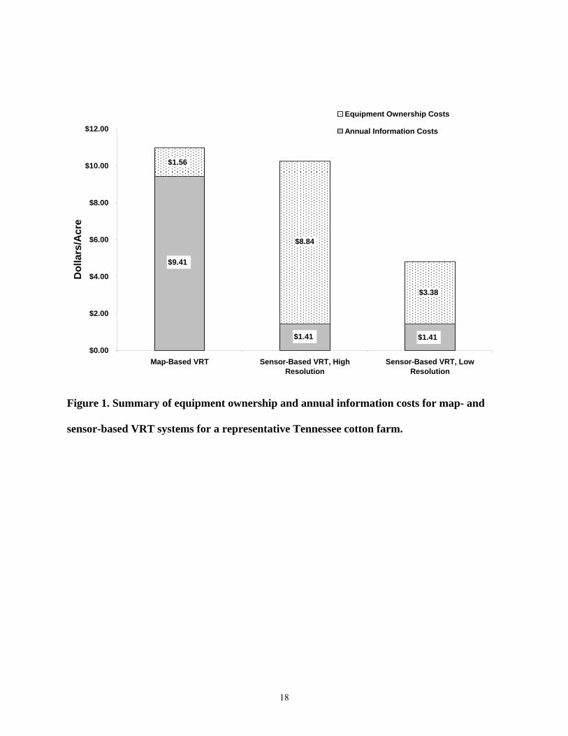
Total per-acre equipment ownership and information costs were $10.97/acre for the map-based

VRT system and $4.79/acre and $10.25/acre for the low- and high-resolution sensor-based VRT

systems, respectively (Figure 1). Despite the similarity in total per-acre cost for the map-based

and high resolution sensor-based systems, the cost structure differed significantly. The map-

based VRT system had high information-gathering costs but low equipment ownership costs. In

contrast, the high-resolution sensor-based VRT system had low information-gathering costs but

high equipment ownership costs.

The difference in per-acre cost estimates between VRT systems is primarily due to the

cost of spatial data collection (Table 1). Ownership costs for the NDVI sensors were $1.82/acre

for the low-resolution kit (20 ft × 30 ft) and $7.28/acre for the high-resolution kit (2 ft × 2ft). The

cost for the high-resolution kit was almost identical to the $7.20/acre aerial imaging cost that was

obtained by allocating 80% of its total initial cost ($9/acre) to sprayer operations. Annualized

ownership costs for the variable rate controller-monitor, GPS, and GIS components are assumed

10

identical regardless of VRT system, for a total cost of $1.56/acre. Similarly, annual information

costs for the GPS signal subscription, GIS software maintenance, prescription map making, data

analysis and training, and labor costs are also assumed identical for all VRT systems for a total

cost of $2.43/acre.

These results highlight the distinguishing characteristics of the two VRT systems

analyzed. Sensor-based systems require a substantial initial investment, but have low recurring

annual costs compared to aerial imaging-based systems. The total initial investment cost for

sensor-based systems was $72,950, which included the high-resolution NDVI sensor kit, variable

rate controller, GPS and GIS components; as compared to $12,950 for the aerial imaging-based

system which had identical equipment except for the NDVI sensors.

Example 2: Medium-Sized West Tennessee Cotton Farm

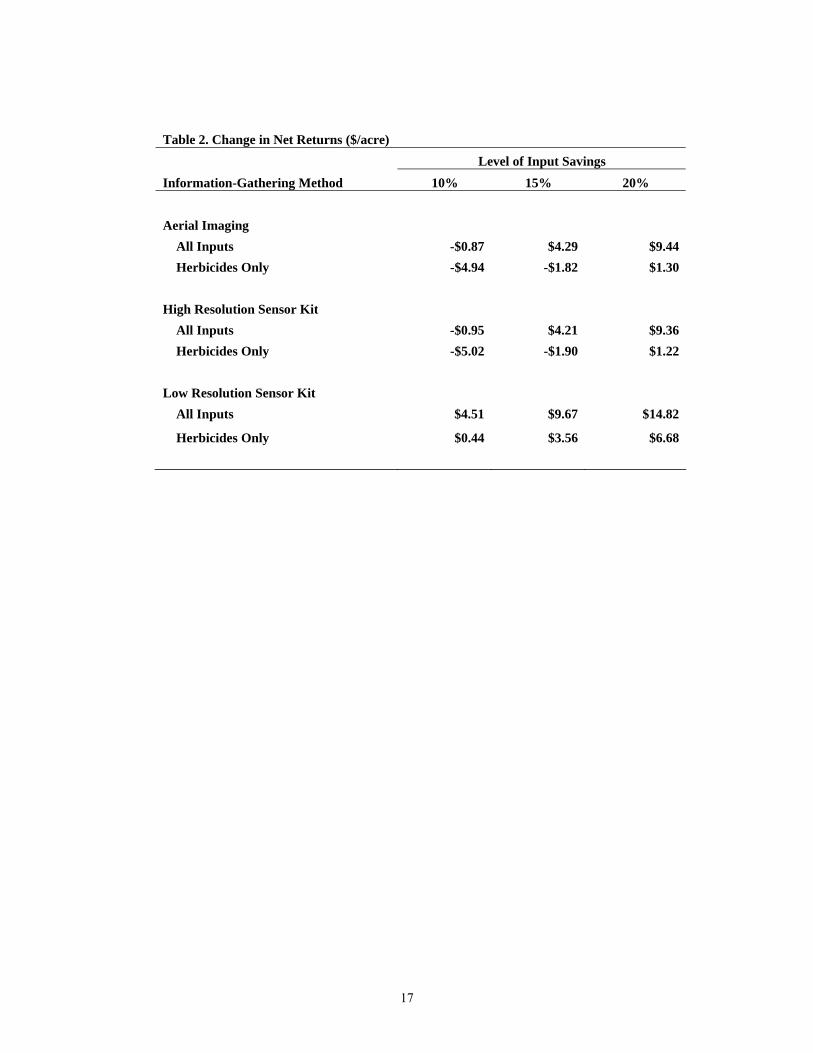
The profitability of the two VRT systems analyzed varied based on the inputs varied and the

level of input savings (Table 2). Considering all sprayer-applied inputs used in cotton

production, results indicated that a 10% level of input cost savings would not be sufficient to pay

for VRT systems utilizing aerial imaging or high-resolution sensors for information-gathering. In

both cases, the breakeven input cost savings is 11%. At a 15% input cost savings level, the

adoption of a VRT system would increase profitability by $4.29/acre using aerial imaging and by

$4.21/acre using high-resolution sensors. Considering the variable rate application of herbicides

only, cost savings of over 15% would be required to pay for the VRT system utilizing aerial

imaging or high-resolution sensor kits. The breakeven herbicide cost savings were 18% for aerial

imaging and 19% for the high-resolution sensors. A 10% level of input savings, however, would

pay for investments in low-resolution sensor kits and would increase profitability by $4.51/acre.

11

The profitability of VRT systems using high-resolution sensor kits for information-

gathering was the most sensitive to the cotton area planted and equipment lifetime (Figure 2). A

cotton area of 600 acres or less, or an equipment lifetime of 5 years or less would result in VRT

investments being unprofitable. This is not surprising due to the large initial investment required

for sensor-based VRT systems. Larger cotton areas or longer useful equipment lifetimes allow

fixed costs to be spread across more acres. An allocation of 100% of costs to the sprayer, or an

increase in the price of the sensor kit to $80,000 would result in positive but much smaller net

returns as compared to the baseline scenario. Net returns were also sensitive to interest rate, VRT

annual costs, and VRT equipment costs, but net returns remained positive even at low values.

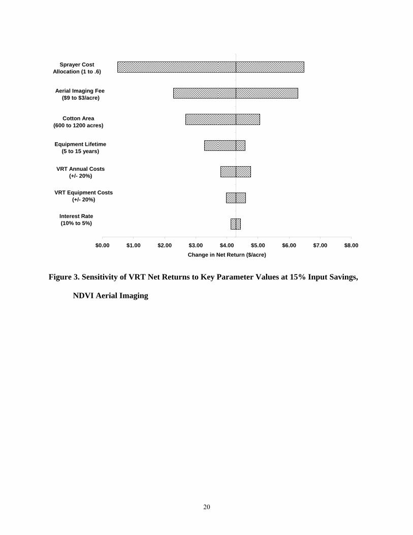
The profitability of VRT systems using aerial imaging was the most sensitive to sprayer

cost allocation, but the change in net returns remained positive across the entire range of values

considered (Figure 3). As compared to sensor-based VRT investments, VRT investments using

aerial imagery for information-gathering were less sensitive to changes in cotton area and aerial

imagery costs. For example, even with aerial imaging fees of $12/acre or a farm size of 600

acres, net returns remain above $2/acre. VRT equipment costs, VRT annual costs, and interest

rate had only a small effect on net returns to cotton production.

Research Summary and Discussion

This paper analyzed the returns required to pay for investments in map- and sensor-based VRT

systems for agricultural sprayers. Two commercially-available VRT systems, one using aerial

imaging and the other using vehicle-mounted sensors, were considered in detail. The profitability

of each system was determined by comparing potential input and application cost savings with

annualized ownership and annual information-gathering costs. The framework was illustrated

using example analyses based on a medium-sized cotton farm in West Tennessee.

12

Sensor-based VRT systems were found to have high ownership costs but low recurring

annual costs. In contrast, map-based VRT systems were found to have lower ownership costs but

higher annual information costs. Under a baseline scenario, VRT systems using high-resolution

NDIV sensors and those using aerial NDVI imagery were found to be become profitable at input

savings levels of 11% or above. The profitability of sensor-based VRT systems was most

sensitive to cotton area planted and the expected useful lifetime of VRT equipment. Increased

cotton area or equipment lifetime allows these fixed costs to be spread across more acres.

Producers with less cotton area, or who expect to use and maintain VRT equipment for fewer

years may find aerial imagery VRT options more attractive.

Another key parameter to consider is the proportion of VRT ownership costs and

information-gathering costs to be allocated to sprayer operations. Sensitivity analyses indicated

that when VRT costs are allocated entirely to sprayer operations, the breakeven level of input

savings required for VRT to pay increased significantly. A producer or custom applicator who is

able to use VRT equipment components and site-specific data for precision agriculture tasks that

are in addition to sprayer operations, such as planting, fertilization, and yield monitoring, would

find VRT systems for agricultural sprayers to be more profitable.

References

American Agricultural Economics Association. 2000. Commodity Costs and Returns Estimation

Handbook. American Agricultural Economics Association, Ames, IA.

Ahrens, W.H. 1994. Relative costs of a weed-activated versus conventional sprayer in northern

Great Plains fallow. Weed Technology 8.

13

Bennett, A.L., and D.J. Pannell. 1998. Economic Evaluation of a Weed-Activated Sprayer for

Herbicide Application to Patchy Weed Populations. Australian Journal of Agricultural

and Resource Economics, 42.

Batte, M. and M.R. Ehsani. 2006. The Economics of Precision Guidance with Auto-Boom

Control for Farmer-Owned Agricultural Sprayers. Computers and Electronics in

Agriculture 53: 28-44.

Boehlje, M.D., and V.R. Eidman. 1984. Farm Management. New York: Wiley and Sons.

Buick, R., and E. White. 1999. Comparing GPS Guidance with Foam Marker Guidance. In:

Proceedings of the Fourth International Conference on Precision Agriculture, eds. R.H.

Rust and W.E. Larson. Madison, WI: ASA/CSSA/SSSA.

Ehsani, M.R., M. Sullivan, and T. Zimmerman. 2002. Field Evaluation of the Percentage of

Overlap for Crop Protection Inputs with a Foam Marker System Using Real-Time

Kinematic GPS. Institute of Navigation 60th Annual Meeting, Dayton, OH.

Ess, D.R., M.T. Morgan, and S.D. Parsons. 2001. Implementing Site-Specific Management: Map

versus Sensor-Based Variable Rate Application. Publication Number SSM-2-W, Site-

Specific Management Center, Purdue University, West Lafayette, IN. Retrieved July, 11,

from http://www.ces.purdue.edu/extmedia/AE/SSM-2-W.pdf.

Gerhards, R., and S. Christensen. 2003. Real-Time Weed Detection, Decision Making, and Patch

Spraying in Maize, Sugarbeet, Winter Wheat, and Winter Barley. Weed Research, 43.

Gerloff, D.C. 2007. Field Crop Budgets for 2007. The University of Tennessee Institute of

Agriculture, Agricultural Extension Service, Knoxville, TN. Retrieved December 11,

2007, from http://economics.ag.utk.edu/budgets.html.

14

Griffin, T., D. Lambert, and J. Lowenberg-DeBoer. 2005. Economics of Lightbar and Auto-

Guidance GPS Navigation Technologies. Department of Agricultural Economics, Site-

Specific Management Center, Purdue University, West Lafayette, IN.

Griffin, T.W., J. Lowenberg-DeBoer, D.M. Lambert, J. Peone, T. Payne, and S.G. Daberkow.

2004. Adoption, Profitability, and Making Better Use of Precision Farming Data. Staff

Paper #04-06. Department of Agricultural Economics, Purdue University, West

Lafayette, IN.

Lambert, D., and J. Lowenberg-DeBoer. 2000. Precision Agriculture Profitability Review. Site-

Specific Management Center, Purdue University, West Lafayette, IN, September 2000.

Retrieved January 11, 2008, from http://www.agriculture.purdue.edu/ssmc.

Larson, J.A., R.K. Roberts, B.C. English, J. Parker, and T. Sharp. 2004. A Case Study Economic

Analysis of a Precision Farming System for Cotton. Proceedings of the Beltwide Cotton

Conferences [San Antonio, TX, 5-9 January 2004], eds., P. Dugger and D. Richter, pp.

539-542. Memphis, TN: National Cotton Council of America, 2004.

Oriade, C.A., R.P. King, F. Forcella, J.L Gunsolus. 1996. A bioeconomic analysis of site-specific

management for weed control. Review of Agricultural Economics, 18, 4.

Rider, T., J. Vogel, J. Dille, K. Dhuyvetter, and T. Kastens. 2006. An Economic Evaluation of

Site-Specific Herbicide Application. Precision Agriculture, 7, 6.

Roberts, R.K., B.C. English, and J.A. Larson. 2006. The Variable-Rate Input Application

Decision for Multiple Inputs with Interactions. Journal of Agricultural and Resource

Economics, 31, 2.

Roberts, R.K., B.C. English, J.A. Larson, R.L. Cochran, W.R. Goodman, S.L. Larkin, M. Marra,

S.W. Martin, K.W. Paxton, W.D. Shurley, and J.M. Reeves. 2006. Use of Precision

15

Farming Technologies by Cotton Farmers in Eleven States. In, Proceedings of the

Beltwide Cotton Conferences [San Antonio, TX, 3-6 January 2006], ed., D. Richter.

Memphis, TN: National Cotton Council of America.

Robinson, E. 2004. Computer whizzes need not apply. Delta Farm Press, February 13, 2004.

Available online at: http://deltafarmpress.com/news/farming_computer_

whizzes_need (verifed 17 Dec 2007).

Solie, J. 2005. GreenSeeker. Selected Presentation, 8th Annual Kansas Precision Agriculture

Technologies Conference. January 19-20, 2005, Hays, KS. Available online at:

http://www.ksagresearch.com/ (verified 17 Jan 2008).

Swinton, S.M. and J. Lowenberg-DeBoer. 1998. Evaluating the Profitability of Site-Specific

Farming. Journal of Production Agriculture, 11.

Tiller, K. and J. Brown. 2002. TN Cotton: Representative Farm Model. Tennessee Financial

Analyses and Risk Management Strategies (TN FARMS) Document. Agricultural Policy

Analysis Center, The University of Tennessee, Knoxville, TN.

U.S. Department of Agriculture, Economic Research Service. 2007. Commodity Cost and

Returns Database. Washington, DC: USDA-ERS. Available online at:

http://www.ers.usda.gov/Data/CostsAndReturns/ (verified 12 Jan 2009).

16

Table 1. Per-Acre Costs for VRT Equipment and Information-Gathering

Item Unit Quantity Purchase Per-Acre Price Cost $/unit $/acre

VRT equipment costs (Annualized) Variable rate controller-monitor item 1 $6,000 $0.73 GPS receiver and antenna item 1 $5,000 $0.61 Computer and GIS software item 1 $1,450 $0.18 Installation item 1 $500 $0.04 NDVI sensor kit (20 x 30 ft resolution) item 1 $15,000 $1.82 NDVI sensor kit (2 ft x 2 ft resolution) item 1 $60,000 $7.28 VRT information gathering costs

NDVI aerial imaging subscription acre 900 $9.00 $7.20 GPS signal subscription fee item 1 $800 $0.71 GIS software maintenance fee item 1 $200 $0.22 Prescription map making acre 900 $1.00 $0.80 Data analysis and training item 1 $700 $0.62 VRT labor costs hours 10 $8.50 $0.08

17

Table 2. Change in Net Returns ($/acre) Level of Input Savings Information-Gathering Method 10% 15% 20% Aerial Imaging

All Inputs -$0.87 $4.29 $9.44 Herbicides Only -$4.94 -$1.82 $1.30

High Resolution Sensor Kit

All Inputs -$0.95 $4.21 $9.36 Herbicides Only -$5.02 -$1.90 $1.22

Low Resolution Sensor Kit All Inputs $4.51 $9.67 $14.82

Herbicides Only $0.44 $3.56 $6.68

18

$1.41

$9.41

$1.41

$3.38

$1.56

$8.84

$0.00

$2.00

$4.00

$6.00

$8.00

$10.00

$12.00

Map-Based VRT Sensor-Based VRT, HighResolution

Sensor-Based VRT, LowResolution

Dol

lars

/Acr

e . .

.

Equipment Ownership Costs

Annual Information Costs

Figure 1. Summary of equipment ownership and annual information costs for map- and

sensor-based VRT systems for a representative Tennessee cotton farm.

19

Interest Rate (5% to 10%)

High Res. Sensor Kit ($40K to $80K)

VRT Equipment Costs (+/- 20%)

VRT Annual Costs (+/- 20%)

Sprayer Cost Allocation (.6 to 1)

Cotton Area (600 to 1200 acres)

Equipment Lifetime (5 to 15 years)

-$4.00 -$2.00 $0.00 $2.00 $4.00 $6.00 $8.00Change in Net Return ($/acre)

Figure 2. Sensitivity of VRT Net Returns to Key Parameters at a 15% Input Savings, NDVI

High-Resolution Sensor Kit

20

Interest Rate (10% to 5%)

VRT Equipment Costs (+/- 20%)

VRT Annual Costs (+/- 20%)

Equipment Lifetime (5 to 15 years)

Cotton Area (600 to 1200 acres)

Sprayer Cost Allocation (1 to .6)

Aerial Imaging Fee ($9 to $3/acre)

$0.00 $1.00 $2.00 $3.00 $4.00 $5.00 $6.00 $7.00 $8.00Change in Net Return ($/acre)

Figure 3. Sensitivity of VRT Net Returns to Key Parameter Values at 15% Input Savings,

NDVI Aerial Imaging