ECONOMIES OF SCOPE OF LENDING AND MOBILIZING DEPOSITSIN RURAL MICROFINANCE INSTITUTIONS: A SEMIPARAMETRIC

ANALYSIS

VALENTINA HARTARSKA, CHRISTOPHER F. PARMETER, AND DENIS NADOLNYAK

Microfinance emerged as an innovation in lending to the rural poor in Asia and in response

to frequent failure of previous interventions in rural financial markets such as directed and

subsidized production credit disbursed by agricultural development banks. While it started

“as a collection of banking practices built around providing small loans (typically without

collateral) and accepting tiny savings deposits” Armendariz de Aghion and Morduch (2005,

p. 1), today many microfinance institutions (MFIs) expand their services and strive to offer

payment and savings facilities, insurance, housing, and longer-term loans to marginalized

clientele in rural and urban settings.

Estimates show that there are at least 10,000 microfinance programs worldwide. Two

related and important trends are now emerging. The first is toward commercialization which

essentially is transforming NGO-MFIs into regulated intermediaries with the intent to lower

costs by accessing deposits as well as strengthen the organizations by privatization. The

second trend is a renewed interest in experimentation to mobilize savings with emphasis on

rural savings. Economies of scope imply that expansion into the savings market can be more

cost efficient if done by the same MFIs, which makes it a significant factor in assessing the

feasibility of these innovations. However, there are few studies that estimate the magnitude

and sign of scope economies. In this paper, we present some preliminary evidence on scope

economies using a large sample of MFIs.

Valentina Hartarska, Corresponding Author, Department of Agricultural Economics and Rural Sociology,Auburn University, USA. Christopher F. Parmeter, Department of Agricultural and Applied Economics,Virginia Polytechnic Institute and State University, USA. Denis Nadolnyak, Department of AgriculturalEconomics and Rural Sociology, Auburn University, USA.

1

Aside from Hartarska, Parmeter and Mersland (2009), we are the first to estimate scope

economies in microfinance. Whereas Hartarska, Parmeter and Mersland (2009) focused on

pure estimation of scope economies and their magnitude across a variety of factors/regions,

we investigate a much more comprehensive list of MFIs in addition to focusing on the distinc-

tion between fixed-cost economies and cost-complementarities. This is important since these

components can provide further insight into the nature and magnitude of scope economies.

In addition, we provide a novel approach to dealing with extreme observations in applied

non/semiparametric settings. This approach has merit regardless of context across economic

subdisciplines.

Our findings indicate that policies designed to improve MFIs’ performance to expand their

services should be based on regional, organizational, and characteristics of the environment

in which MFIs operate. The analysis suggests that economies of scope are driven mostly

by fixed cost sharing while we do not find cost complementarities in most regions and MFI

types.

The plan of the paper is as follows. We first discuss the theoretical and econometric

techniques needed to estimate scope economies. We then proceed to detail the MFI data

which we use in this study. Next, the results from our econometric investigation are present

while conclusions and direction for future research finish our paper.

Estimation of economies of scope

Pulley and Humphrey (1993) define overall economies of scope as the percentage of cost

savings from producing all outputs jointly as opposed to producing each output separately.

Here we have only two outputs (q1, and q2), loans and deposits, so our estimates of scope

economies are:

(1) SCOPE =C(q1, 0; r̄) + C(0, q2; r̄)− C(q1, q2; r̄)

C(q1, q2; r̄),

2

where r̄ is a vector of ` input prices (here taken to be the relative price of labor and borrowed

funds), and C(·) is the cost function. Given that the data used to estimate the cost function

will represent a mix of firms producing loans and deposits jointly and firms specializing

in the production of loans exclusively, the use of standard cost functions in production

econometrics are not suitable. For example, the transcendental logarithmic cost function

(Christiansen, Jorgensen and Lau 1971) cannot directly handle zero outputs. Thus, the use

of a logarithmic style cost function for the study of economies of scope is in general restrictive

and inappropriate for a wide array of empirical problems.1

An empirical cost function for estimating scope economies was suggested by Pulley and

Braunstein (1992, PB hereafter) based on of the theoretical cost function suggested by Bau-

mol, Panzer and Willig (1982). Their cost function is multiplicatively separable in outputs

and input prices and is quadratic (as opposed to log-quadratic) in outputs, thus alleviating

the empirical issue of zero valued outputs in real world data sets. The composite cost model

of PB can be written more succinctly as

(2) C(q, ln r) = F (q, ln r) · G̃(ln r) + u.

Semiparametric Smooth Coefficient Cost Function

The empirical model of PB reflects a composite structure suitable for estimating scope

economies, Asaftei, Parmeter and Yuan (2009) recently proposed a semiparametric smooth

coefficient cost function (SPSCC) that takes a similarly representative form but relaxes the

specific functional form restrictions on G̃(ln r).2 This setup, with the same type of cost

structure for F (q, ln r), affords the researcher sufficient flexibility to model costs and investi-

gate scope economies. While the theoretical properties of cost functions are well known with

traditional input prices, the use of environmental variable is less well understood. Thus, the

ability to introduce these variables in a manner that imposes little structure on their exact

3

specification within the cost function is pertinent. Additionally, given the importance of en-

vironmental factors on microfinance institutions (Armedariz and Szafarz 2009), our ability

to control these influences in a general way is desirable.

We can write equation (2) in the following SPSCM specification,

(3) yi = α(zi) + β(zi)xi + εi

where yi ≡ Ci, xi = [1 q′i qq′i q ln r′i]′, zi = [ln ri Vi] and where qi represents the vector of

outputs for the ith firm, ri is the vector of input prices and Vi encapsulate our environmental

variables. Here, qq′i is the k(k− 1)× 1 vector of squares and interactions of the outputs and

q ln r′i is the kj × 1 vector of interactions between outputs and log input prices.

Another way to think of this model is that for a given level of zi, we have a linear-in-

parameters model where the slopes possibly differ for differing levels of zi. SOne can view

the original PB model as a smooth coefficient model.The key difference between the semi-

parametric smooth coefficient model in equation (3) and the parametric smooth coefficient

model of PB is that the coefficients are identical, up to scale, in the parametric model

proposed by PB while in equation (3) they can be entirely different functions altogether.

Li et al. (2002) and Li and Racine (2009) proposed an estimation procedure for the SPSCM

defined in equation (3) based on local constant least squares (LCLS). The estimation of

equation (3) is as follows. Denote δ(zi) = [α(zi), β(zi)] and rewrite (3) as yi = δ(zi)Xi + εi,

where Xi = [1 xi]. Our LCLS estimator of δ(z) becomes

(4) δ(z) = (X′K(z)X)−1X′K(z)y,

where K(z) is a diagonal matrix with ith element Ki = Kγ(zi, z) and X is our matrix

composed of Xi. Ki is constructed using the generalized product kernel of Racine and Li

(2004) and γ is a vector of bandwidths.3 The reason we use a generalized kernel is that

several of our environmental variables are discrete,4 most notably our indicator for loan

4

method and area serviced by the MFI. Smoothing these types of variables with continuous

kernels is inappropriate while treating it as a dummy variable leads to a loss of efficiency in

our estimates of the smooth coefficients.

Fixed and Complementary Costs

Once we have estimated our SPSC cost function we can easily obtain scope economies from

(1) as

(5) SCOPE =α(z)− β1,2(z)q1q2

TC,

where β1,2(z) is the coefficient on the interaction between the two outputs produced by

MFIs and TC represents estimated total costs. We can decompose α(z) into two separate

components to obtain the contribution of fixed costs to our scope economies. That is, since

input prices are a component of z, we have to evaluate α(z) at 0 input prices, holding the

remaining environmental variables fixed to obtain a ‘true’ intercept representing fixed costs.

Thus, we can break up our intercept as

(6) α(z) = α(0, z−) + (α(z)− α(0, z−)) .

Here the notation z− is taken to mean our original z vector excluding input prices, which

have been set to zero.

Using this division of our intercept we can decompose scope economies into fixed and

complementary cost components. We have

SCOPE =α(0, z−) + (α(z)− α(0, z−))− β1,2(z)q1q2

TC

=α(0, z−)

TC+

(α(z)− α(0, z−))− β1,2(z)q1q2

TC

=SCOPEFC + SCOPECC .(7)

5

Scope economies arise through fixed costs by spreading costs over an expanded set of outputs

whereas scope economies arise through cost complementarities if variable inputs are shared

across alternative outputs. Specifically, cost complementarities accrue to MFIs if the account

information that is developed in the process of creating deposits is subsequently used to help

monitor and gather credit information on loans for the same customer base. Spreading

fixed costs over an enhanced product base produces scope economies if the same set of tools

required to manage deposits can also be used to produce and monitor loans.

Data

The data were collected from the MIXMARKET database on November 1st 2008. At that

time, the database consisted of over 1,300 MFIs. Most MFIs had data for several years with

the maximum of eight. After dropping all observations that did not have sufficient data for

calculating the cost function, the dataset included 882 MFIs with the average of about 3

years of data, or 2,712 total annual observations where output is measured by the number

of clients. These observations represent 93 countries. The data cover the period 1998-2007.

Although the data are self-reported, most MFIs that disclosed the detailed data necessary

for the calculation of a cost function are considered high quality with a MIXMARKET

rating of three stars (78%), which marks that an MFI has at least two years of financial and

outreach data reported or a rating of four stars (33%), which marks an MFI with audited

financial statements. All values are in US dollars.

Total cost is the sum of financial and operating expenses. Salary is the ratio of operating

expenses divided by the number of employees while financial costs are defined as the ratio of

financial expenses to liability (this measure incorporates the cost of both loans and deposits

measured at the actual price paid by the MFI). Financial depth is the ratio of the money

aggregate including currency, deposits, and electronic currency (M3) over GDP and measures

the level of financial development. Rural population is the proportion of people living in rural

areas in the country in which the MFI operates while population density is the number of

people per square kilometer.

6

Given that the data were not directly available they were calculated using the methodology

proposed by Hermes, Lensink and Meesters (2009). Therefore, it is expected that outliers

are present and we provide an easily implementable empirical procedure to mitigate their

effects on the analysis.

Summary statistics of the variables used in the scope estimation are listed in Table 1. #

of Borrowers represents the number of active borowers and # of Savers the number of active

savers. The average number of borrowers is 58,000 but the rage is huge - from 9 to over 6

million borrowers and up to 32 million savers. The average ratio of operating expense per

staff member (salary) is $12,933 and ranges from just under two to more than $121,000 (see

table 1 for more details).

[PLACE TABLE 1 APPROXIMATELY HERE]

Results

For the model discussed in the previous section we estimate a SPSCM cost function with two

outputs and two input prices. Input prices are scaled by labor costs to produce a relative

capital labor price. Total costs, # of loans and # of deposits are all scaled by 1,000,000

to stabilize the smooth coefficients during bandwidth selection. All results were computed

using the np package (Hayfield and Racine 2008) in R (R Development Core Team 2008).

In addition to normalized input prices entering the unknown smooth coefficients, we also

included the year in which the MFI was observed and its region, the type of operation the

MFI falls under, the population density and proportion of rural population in the country

where the MFI operates and the level of financial depth. This addresses recent concerns

that in cross-country studies environmental factors affect MFI’s operations (Armedariz and

Szafarz 2009). Given our ability to smooth discrete variables (year, MFI type and region) we

employ discrete kernels (see Li and Racine 2007) for these variables and standard Gaussian

kernels for the remaining continuous variables.

Robust cross validation

7

In the process of estimating the bandwidths we noticed that the least squares cross validation

(LSCV) criteria was extremely sensitive to the presence of outliers (see Leung 2005). To

remedy this we used the suggestion of Henderson and Kumbhakar (2006, footnote 4) and

removed outliers prior to estimating the bandwidths via LSCV.5 These outliers were then

used to estimate scope economies.

To determine outliers we tried several different approaches couched in terms of distance-

based methods. The simplest approach is to create a robust version of the Mahalanobis

distance:

RDi =√

(xi − µ)′C−1(xi − µ),

where µ is a robust estimate of the mean of the data (used for smoothing) and C is a

robustly estimated covariance matrix. The approach of Rousseeuw and van Driessen (1999)

estimates C such that C has the smallest determinant and contains at least J points. J

in this setting represents the robustness of the covariance matrix estimator. Alternatively,

one could employ the recent outlier detection method of Filzmoser, Maronna and Warner

(2008). A novel feature of this approach is that it uses principal component analysis which

allows faster computation and provides better outlier detection in high dimensions. 6

Roughly 10% of our estimates of scope economies were over 100% in magnitude. These

estimates drastically affect the mean estimates and, in some cases, the upper and lower

quartiles. Therefore, in this section, we present primarily our results obtained from the

dataset excluding these extreme estimates. We note that our qualitative results are robust

to whether these estimates are included or not.7

Scope Economies

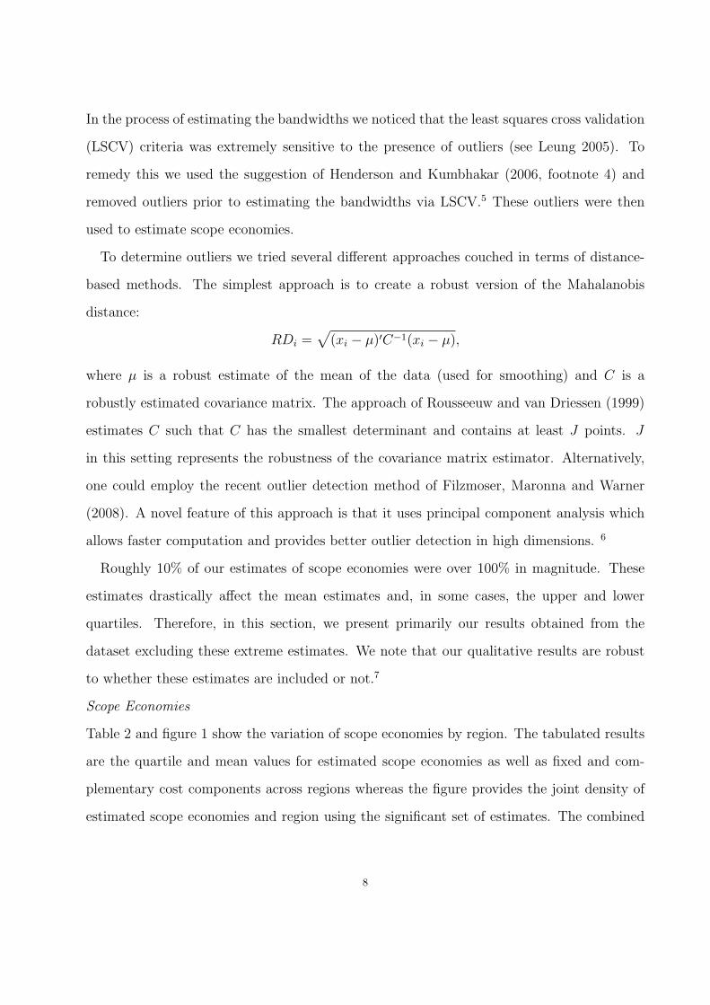
Table 2 and figure 1 show the variation of scope economies by region. The tabulated results

are the quartile and mean values for estimated scope economies as well as fixed and com-

plementary cost components across regions whereas the figure provides the joint density of

estimated scope economies and region using the significant set of estimates. The combined

8

economies of scope appear to be the highest in the Middle East and in Eastern Europe and

the lowest in Latin America and Africa.

[PLACE TABLE 2 and FIGURE 1 APPROXIMATELY HERE]

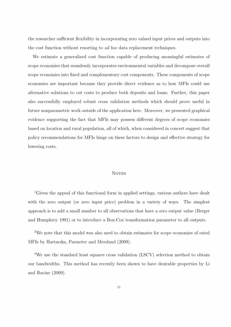
Table 3 and figure 2 provide a more in-depth analysis of how scope economies vary by

MFI type.8 The figure provides the joint density of estimated scope economies and MFI

type using the significant set of estimates. While typically MFIs classified as non-profits and

non-bank financial institutions do not offer savings/deposits, they seem to be the ones with

the highest potential for realizing scope economies.

[PLACE TABLE 3 AND FIGURE 2 APPROXIMATELY HERE]

Of particular interest in this analysis is the relation of scope economies to the proportion

of rural population in the country as there is substantial interest in offering savings in rural

areas and scope economies may contribute to its feasibility. Joint density plots of estimated

scope economies and rural population density (figures not shown due to space limitations)

suggest that economies of scope are non-linear and peak for MFIs in countries with about

70-75 percent of rural population. Further decomposing the estimated joint densities by MFI

type, we focus on Non-Profit and Non-Bank MFIs as these splits are the largest groups. We

find that scope economies are higher for non-banks whereas, for non-profits, the landscape is

more sensitive to changes in the rural population. However, this result should be interpreted

with caution because, in comparison to banks, both non-banks and non-profits are usually

under-represented in rural areas.

The general conclusion from further analysis is that environmental/external factors mat-

ter for scope economies which vary by geographical region and by population mix. When

diseconomies of scope are present, savings comes with its own added cost. We find evidence

of some diseconomies of scope present in non-profits (particularly in more urban countries).

In Africa, the diseconomies increase with the share of rural population, whereas in Latin

America and Asia the diseconomies transpire mostly in the more urban countries.

Scope Economies Components

9

For a better understanding of the nature of scope economies in microfinance, we look at

its main components - the fixed cost and complementary costs scope economies - by both

MFI type and region with respect to rural population densities. The results show where

economies of scope are arising across a variety of strata as well as how they differ based on

where and how the MFI is setup. This information is important for policy design aimed at

improving MFI operations.

In table 4 the first block is for all of estimates whereas the second block is for our estimates

which are deemed statistically significant when paired with their corresponding standard

errors at the 1% level. While, on average, the scope economies are positive, there are some

diseconomies that are much higher in the complementary cost component.

[PLACE TABLE 4 APPROXIMATELY HERE]

Density plots of scope economies by MFI type (not shown), as well as table 3, suggest that

the scope economies are mostly due to fixed cost sharing and that non-profit, non-bank, and

cooperative MFIs (in that order) possess highest scope economies due to fixed cost sharing.

Figure 3 shows the relation between the nature of scope economies and rural population

density in non-profits and non-bank MFIs.9 Density shapes suggest that, for both non-

bank financial institutions and non-profit MFIs, the fixed costs component becomes more

important in countries with more rural population. The diseconomies of scope, when present,

are the highest in the complementary cost component.

[PLACE FIGURE 3 APPROXIMATELY HERE]

Conclusions

While economies of scope of lending and mobilizing deposits in banking are justified the-

oretically (Diamond 1984) and found empirically (see Sounders 1999), in microfinance the

existence and magnitude of scope economies has not been investigated. We use a semipara-

metric smooth coefficient model to estimate these economies using a dataset put together

from MFIs with over 2700 annual observations from across the globe. This model affords

10

the researcher sufficient flexibility in incorporating zero valued input prices and outputs into

the cost function without resorting to ad hoc data replacement techniques.

We estimate a generalized cost function capable of producing meaningful estimates of

scope economies that seamlessly incorporates environmental variables and decompose overall

scope economies into fixed and complementary cost components. These components of scope

economies are important because they provide direct evidence as to how MFIs could use

alternative solutions to cut costs to produce both deposits and loans. Further, this paper

also successfully employed robust cross validation methods which should prove useful in

future nonparametric work outside of the application here. Moreover, we presented graphical

evidence supporting the fact that MFIs may possess different degrees of scope economies

based on location and rural population, all of which, when considered in concert suggest that

policy recommendations for MFIs hinge on these factors to design and effective strategy for

lowering costs.

Notes

1Given the appeal of this functional form in applied settings, various authors have dealt

with the zero output (or zero input price) problem in a variety of ways. The simplest

approach is to add a small number to all observations that have a zero output value (Berger

and Humphrey 1991) or to introduce a Box-Cox transformation parameter to all outputs.

2We note that this model was also used to obtain estimates for scope economies of rated

MFIs by Hartarska, Parmeter and Mersland (2009).

3We use the standard least squares cross validation (LSCV) selection method to obtain

our bandwidths. This method has recently been shown to have desirable properties by Li

and Racine (2009).

11

4Let zi = [zdi , z

ci ], where zd

i is a vector of discrete regressors and zci is a vector assuming

continuous values. One can further decompose zdi into subvectors of ordered and unordered

discrete regressors, zdoi and zdu

i , respectively.

5Henderson and Kumbhakar (2006) only mentioned, but did not actually report their

results from, this approach in their work so this marks the first reported application of this

insight on a form of robust cross-validation.

6Both of the methods described here, as well as others, can be accessed in R via the pack-

ages “mvoutlier” (Gschwandtner and Filzmoser 2009) and “robustbase” (Maechler 2009).

7Results including these extreme estimates are available upon request.

8Rural banks classification is only for MFIs in Indonesia while banks serving predomi-

nantly rural clients are not classified as rural banks by the MIXMARKET in other countries.

The category Other (MFIs without a category assigned to them by MIXMARKET) is less

than one percent. These two categories represent less than 5 percent of the sample and are

excluded from the analysis.

9The densities were constructed using the Gaussian kernel and rule-of-thumb bandwidths.

References

Armedariz, B. and A. Szafarz (2009), On mission drift in microfinance institutions. Paper presented at the

First European Research Conference on Microfinance, Brussels, Belgium.

Armendariz de Aghion, B. and J. Morduch (2005), Microeconomics of Microfinance, MIT Press.

Asaftei, G., C. F. Parmeter and Y. Yuan (2009), Economies of scope in financial services: A semi-parametric

approach. Virginia Tech Working Paper.

Baumol, W. J., J. Panzer and R. Willig (1982), Contestable Markets and the Theory of Market Structure,

Harcourt, New York.

Berger, A. and D. Humphrey (1991), ‘The dominance of inefficiences over scale and product mix economies

in banking’, Journal of Monetary Economics 28, 117–148.

12

Christiansen, L. R., D. W. Jorgensen and L. J. Lau (1971), ‘Conjugate duality and the transcendental

logarithmic production function’, Econometrica 39, 255–256.

Diamond, D. (1984), ‘Financial intermediation and delegated monitoring’, Review of Economic Studies

51, 393–414.

Filzmoser, P., R. Maronna and M. Warner (2008), ‘Outlier identification in high dimensions’, Computational

Statistics and Data Analysis 52, 1694–1711.

Gschwandtner, M. and P. Filzmoser (2009), mvoutlier: Multivariate outlier detection based on robust methods.

R package version 1.4.

*http://www.r-project.org

Hartarska, V., C. F. Parmeter and R. Mersland (2009), Scope economies in microfinance: Evidence from

rated MFIs. Virginia Tech Working Paper.

Hayfield, Tristen and Jeffrey S. Racine (2008), ‘Nonparametric econometrics: The np package’, Journal of

Statistical Software 27(5).

*http://www.jstatsoft.org/v27/i05/

Henderson, D. J. and S. C. Kumbhakar (2006), ‘Public and private capital productivity puzzle: A nonpara-

metric approach’, Southern Economic Journal 73(1), 219–232.

Hermes, N. R., R. Lensink and A. Meesters (2009), ‘Outreach and efficiency of microfinance institutions’,

World Development . Forthcoming.

Leung, D. H.-Y. (2005), ‘Cross-validation in nonparametric regression with outliers’, The Annals of Statistics

33(5), 2291–2310.

Li, Q., C. J. Huang, D. Li and T.-T. Fu (2002), ‘Semiparametric smooth coefficient models’, Journal of

Business & Economic Statistics 20, 412–422.

Li, Q. and J. Racine (2007), Nonparametric Econometrics: Theory and Practice, Princeton University Press.

Li, Q. and J. S. Racine (2009), ‘Smooth varying-coefficient estimation and inference for qualitative and

quantitative data’, Econometric Theory . Forthcoming.

Maechler, M. (2009), robustbase: Basic robust statistics. R package version 0.4-5.

*http://www.R-project.org

Pulley, L. B. and D. Humphrey (1993), ‘The role of fixed costs and cost complementarities in determining

scope economies and the cost of narrow banking proposals’, Journal of Business 66, 437–462.

Pulley, L. B. and Y. M. Braunstein (1992), ‘A composite cost function for multiproduct firms with an

application to economies of scope in banking’, The Review of Economics and Statistics 74, 213–230.

13

R Development Core Team (2008), R: A Language and Environment for Statistical Computing, R Foundation

for Statistical Computing, Vienna, Austria. ISBN 3-900051-07-0.

*http://www.R-project.org

Racine, J. S. and Q. Li (2004), ‘Nonparametric estimation of regression functions with both categorical and

continuous data’, Journal of Econometrics 119(1), 99–130.

Rousseeuw, P. J. and K. van Driessen (1999), ‘A fast algorithm for the minimum covariance determinant

estimator’, Technometrics 41(3), 212–223.

Sounders, A. (1999), Financial Institutions Management, 3 edn, Irwin/McGraw-Hill.

14

Table 1: Summary Statistics For MFI Data.

Variable Mean Std. Dev. Min Median Max

# Borrowers 61701.959 353893.455 9 8529.5 6397635

# of Savers 111617.414 1505987.318 0 0 32252741

Total Cost 5651212.031 35749638.418 0 908590.160 835000000

Financial Costs 0.098 0.167 0 0.062 2.72

Salary 12933.108 10581.880 1.784 10879.459 121204.09

Financial Depth 0.418 0.257 0.070 0.372 2.34

Pop. Density 130.710 196.875 2 64 1109

Rural Pop. 51.594 19.824 6.6 50.020 87.98

MFI Type

Bank 0.067 – 0 – 1

Cooperative 0.176 – 0 – 1

Non-Bank 0.328 – 0 – 1

Non-Profit 0.378 – 0 – 1

Rural 0.034 – 0 – 1

Other 0.018 – 0 – 1

15

Table 2: Quartile And Mean Estimates of Scope Economies And Its ComponentsBy Region.

Q1 Q2 Q3 Mean Q1 Q2 Q3 Mean

Africa Latin America

SCOPE 0.009 0.228 0.529 0.245 −0.098 0.013 0.290 0.105

(0.194) (0.223) (0.131) (0.100) (0.201) (0.359) (8.276) (32.917)

SCOPEFC −0.003 0.182 0.514 7.380 −0.190 −0.021 0.175 −0.039

(0.241) (0.156) (0.174) (2.182) (11.410) (0.187) (0.105) (0.434)

SCOPECC −0.228 0.008 0.125 −6.380 −0.013 0.034 0.165 0.144

(0.077) (0.045) (0.055) (2.182) (0.167) (0.036) (128.634) (2.613)

Asia Middle East

SCOPE −0.009 0.294 0.711 0.327 0.236 0.861 0.999 0.638

(0.026) (3.309) (0.501) (5.945) (0.281) (0.065) (0.000) (0.038)

SCOPEFC 0.084 0.411 0.947 1.279 0.189 0.525 0.971 0.536

(0.068) (0.113) (0.177) (2.538) (2.483) (0.174) (0.045) (0.139)

SCOPECC −0.528 −0.095 0.055 −0.943 −0.047 0.011 0.094 0.092

(1.760) (2.265) (3.413) (4.163) (0.040) (0.030) (0.025) (0.044)

Eastern Europe

SCOPE 0.071 0.365 0.759 0.384

(0.155) (0.174) (0.701) (0.094)

SCOPEFC 0.095 0.370 0.747 0.501

(0.137) (2.884) (1.152) (0.665)

SCOPECC −0.076 0.011 0.066 −0.115

(0.051) (0.134) (1.149) (0.579)

16

Figure 1: Joint Density Of Estimated Scope Economies And Region.

AfricaEast AsiaEastern EuropeLatin AmericaMiddle EastSouth Asia

0.0

0.1

0.2

0.3

0.4

0.5

0.0

0.2

0.4

0.6

0.8

1.0

Region

Econom

ies o

f S

cope

Join

t D

ensity

17

Figure 2: Joint Density Of Estimated Scope Economies And MFI Type.

BankCoOperativeNon−BankNon ProfitOtherRural

0.0

0.2

0.4

0.6

0.8

0.0

0.2

0.4

0.6

0.8

1.0

MFI−Type

Eco

no

mie

s o

f S

co

pe

Jo

int

De

nsity

18

Table 3: Quartile And Mean Estimates Of Scope Economies And Its ComponentsBy MFI Type.

Q1 Q2 Q3 Mean Q1 Q2 Q3 Mean

Bank Non-Profit

SCOPE −0.128 0.020 0.227 0.061 −0.060 0.148 0.633 0.236

(0.059) (0.087) (0.188) (0.078) (1.991) (2.634) (0.207) (14.379)

SCOPEFC −0.017 0.040 0.141 0.092 −0.104 0.124 0.565 0.500

(0.025) (0.114) (0.091) (0.516) (0.320) (3.346) (0.179) (0.198)

SCOPECC −0.105 0.001 0.069 −0.035 −0.123 0.032 0.203 −0.258

(0.228) (0.046) (0.046) (0.270) (0.120) (0.016) (0.209) (0.083)

Cooperative Non-Bank

SCOPE −0.039 0.181 0.553 0.228 0.015 0.250 0.658 0.324

(0.220) (0.175) (0.080) (0.360) (0.203) (3.787) (0.915) (0.411)

SCOPEFC −0.023 0.189 0.547 0.327 0.010 0.281 0.725 0.460

(0.425) (0.324) (0.622) (0.128) (0.126) (0.385) (0.055) (8.089)

SCOPECC −0.069 0.039 0.136 −0.101 −0.128 −0.010 0.036 −0.136

(0.189) (0.125) (0.143) (0.146) (2.294) (0.025) (0.025) (0.833)

19

Table 4: Quartile And Mean Estimates Of Scope Economies And Its Components.

All Estimates Statistically Significant Estimates

Q1 Q2 Q3 Mean Q1 Q2 Q3 Mean

SCOPE −0.025 0.193 0.606 0.264 0.479 0.726 0.947 0.687

(0.081) (0.093) (0.196) (0.270) (0.091) (0.041) (0.034) (0.028)

SCOPEFC −0.023 0.180 0.618 5.304 0.347 0.682 1.020 16.610

(0.197) (0.151) (7.357) (0.235) (0.112) (0.099) (0.127) (3.421)

SCOPECC −0.119 0.007 0.113 −5.004 −0.208 0.011 0.163 −15.703

(0.424) (0.013) (1.031) (1.503) (0.316) (0.019) (0.613) (3.439)

20

Figure 3: Joint Density Of Estimated Scope Economies Components And RuralPopulation By Type.

0.0

0.5

1.0

5560

6570

7580

0.005

0.010

0.015

Economies of Scope (Fixed Cost)

Rural Pop.

Join

t D

en

sity

(a) Non-Banks, Fixed Costs

−1.0

−0.5

0.0

0.5 5560

6570

7580

0.01

0.02

0.03

0.04

0.05

0.06

Economies of Scope (Complementary Cost)

Rural Pop.

Join

t D

en

sity

(b) Non-Banks, Complementary Costs

−0.5

0.0

0.5

1.0

1.545

5055

6065

7075

0.005

0.010

0.015

0.020

Economies of Scope (Fixed Cost)

Rural Pop.

Join

t D

en

sity

(c) Non-Profits, Fixed Costs

−1.0

−0.5

0.0

0.5 5560

6570

7580

0.005

0.010

0.015

0.020

0.025

Economies of Scope (Complementary Cost)

Rural Pop.

Join

t D

en

sity

(d) Non-Profits, Complementary Costs

21