eCOOP : Applying Dynamic Coalition Formation to thePower Regulation Problem in Smart Grids

Radu-Casian Mihailescu

Malmo University, School of TechnologyInternet of Things and People Research Center

Malmo, Sweden

Sascha Ossowski

Rey Juan Carlos UniversityCentre for Intelligent Information Technologies

Madrid, Spain

Matthias Klusch

German Research Center for Artificial Intelligence (DFKI)Saarbruecken, Germany

Abstract

In this work we focus on one particular area of the smart grid, namely,the challenges faced by distribution network operators in securing the balancebetween supply and demand in the intraday market, as a growing number ofload controllable devices and small-scale, intermittent generators coming fromrenewables are expected to pervade the system. We introduce a multi-agentdesign to facilitate coordinating the various actors in the grid. The underpinningof our approach consists of an online cooperation scheme, eCOOP, where agentslearn a prediction model regarding potential coalition partners and thus, canrespond in an agile manner to situations that are occurring in the grid, bymeans of negotiating and formulating speculative solutions, with respect to theestimated behavior of the system. We provide a computational characterisationfor our solution in terms of complexity, as well as an empirical analysis againstreal consumption datasets, based on the macro-model of the Australian energymarket, showing a performance improvement of about 17%.

Keywords:Multi-agent systems, Smart electricity grids, Power regulation, Dynamiccoalition formation

Email addresses: radu.c.mihailescu@mah.se (Radu-Casian Mihailescu),sascha.ossowski@urjc.es ( Sascha Ossowski), matthias.klusch@dfki.de ( MatthiasKlusch)

March 21, 2016

1. Introduction

Recent years have seen the advent of distributed energy resources (DERs)with particular emphasis on clean generation of electricity, predominantly basedon wind and solar power [9]. Albeit representing a sustainable form of energy,renewables pose a major challenge to current electricity networks due to theirstochastic behavior. DERs are essentially characterised by small-scale, intermit-tent and highly unpredictable output. In this context, embedding such devicesin the ageing infrastructure of distribution networks requires novel approachesfor managing the grid efficiently [12, 10]. Given this setting, the organizationof the exchange electricity markets is also expected to change.

Currently, the majority of all power is being traded in what is known asthe day-ahead spot market. Here, the following day is discretized over hourlytime intervals and the market is cleared the day before, fixing the prices andvolumes for the contracted amount of energy. In addition, shortages or ex-cesses of energy are mitigated over the intraday market, which is cleared justbefore the actual power is delivered by producers. Such circumstances mayinclude (but are not limited to) compensating for errors in renewable energyforecasts, smoothing start-up ramps of conventional power plants, correctinginstantaneous mismatches between supply and demand and providing short-term contingency power in case of generator or transmission line failures.

Thus, as the network is becoming more reliant on the power generated byDERs, the role of the intraday market is expected to gain significant importance[3]. The goal is then to maximise the usage of clean energy upon its availabilityand maintain the delicate balance between supply and demand in real-time. Inorder to do so, demand should be able to adapt to the volatility in supply. Thiscan be achieved assuming the flexibility of consumer to adapt their demandbased on incentives provided by the grid operator. Moreover, the system oughtto react in real-time to sudden changes of the aggregated generation profile inorder to balance supply from intermittent renewable resources, while complyingwith consumer requirements. In this paper we address the above-identified re-quirements by proposing a dynamic coalition formation (DCF) algorithm, whereagents representing consumer provide a bottom-up resolution for contingenciesvia a coordinated look-ahead response.

The organization of the rest of this paper is as follows. In Section 2 we reviewsome of the related work. Section 3 introduces a new formalism for the intradaypower regulation problem in terms of a dynamic coalition formation analysis.We then provide in Section 4 the eCOOP control scheme for the same problem,addressing the challenges of an efficient payoff allocation and augmenting ourapproach in the context of privacy preservation. Finally, Section 5 provides anempirical evaluation of our scheme. Section 6 concludes.

2

2. Related Research

Given that the actors participating in the grid (i.e. consumer loads, dis-tributed generators) represent different owners with particular, possibly con-flicting user goals and behaviors, deploying an agent-based distributed controlover the system holds as the natural approach for our scenario [27]. In this workwe aim to apply the multi-agent paradigm to devise a mechanism that enableslocal adaptability to dynamic situations at runtime and allows coordination, asopposed to the more complex task of centralised management [16].

Similar to our work, multi-agent systems have been proposed in the smartgrid domain for the task of demand-side management in a number of studies [33,36, 28]. Critical peak pricing or spot pricing mechanisms attempt to incentivizeagents to adapt their demand, by reducing consumption during peak times [22].Of course, this may end up in situations where peaks are only temporarilyflattened and then shifted to different time intervals, as some of the researchhas shown [32, 28]. More sophisticated solutions have proposed game-theoreticframeworks, [21, 2], for a coordinated adaptation of the agents’ behavior.

Power regulation is however distinct, in that the objective of a correctiveaction is well defined and localized to a particular region of the grid. Peakloadand contingency periods are typically handled by means of adapting the powersupply, by firing expensive, carbon-intensive, peaking plant generators. Instead,here, the grid operator provides a request to consumers for a specific powerregulation action that needs to be addressed in a timely fashion. While demand-side management may be regarded as a day-ahead scheduling problem, for gridregulation, the response time is constrained within minutes, or to even a coupleof seconds.

Due to these challenges, the majority of current methods have been limitedto propose solutions that can only be applied in the day-ahead market. Forinstance, in [35], the authors explore the idea of coupling generation from windfarms with storage facilities, particularly batteries from electric vehicles. Fur-thermore, the approach follows the assumption of a hierarchical organization,where a group leader computes an optimised schedule to maximize profit, for afixed number of given participants. In a similar approach, in [7], the authorsconsider a single owner for the entire system that allows the use of centralisedcontrol, based on dynamic programming scheduling.

More relevant to our context, in [13], the authors report some preliminarywork on deploying electric vehicles (EVs) for power management in the grid.However, they restrict their study to a small-scale scenario, also assuming cen-tralized control over the set of EVs. This eludes some of the harder problemsof operating within limited information environments, where the assumptionsof global knowledge and top-down control of centralization no longer hold.

One of the best practices deployed so far to reduce system peak load is rep-resented by the category of direct load control (DLC) approaches, which imposea brute-force on/off strategy to control loads. In [38], the authors report on astudy in cooperation with the Taiwan Power Company, where to achieve DLCthey use a multi-pass dynamic programming method to schedule the operation

3

of air conditioners in order to reach peak reduction and maximum cost sav-ings. Another DLC scheduling solution is given in [23], where the goal is thatof increasing the profit of the utility using a linear programming algorithm.Recognizing the importance of taking user preference and comfort into account,some DLC solutions [30, 39] deploy a logic-based system to model, by means offuzzy variables, the flexibility of interrupting the air-conditioners and electricwater heaters, in an attempt to factor user satisfaction into their model.

Clearly, the above-mentioned approaches pose a series of limitations. DLCmethods, although already implemented and in use by some energy companies1,assume full control over the consumer loads, which can be exercised at will.There is still an inconclusive debate about whether such approaches are actuallygoing to reach mass adoption, especially in the domestic sector where consumerare often reticent to comply with such energy usage violations. Centralisedsolutions which assume a single owner of the system that has full control over theoperation of all loads is evidently not applicable to instances where participantsare self-interested stakeholders. Finally, applying various pricing schemes hasalso been shown to deliver poor results. For example, individual consumers mayunilaterally decide to shift consumption from expensive time slots to cheap timeslots, thus replacing peaks from one period to another. The problem here is dueto consumers i) not having a clear perception of the amount of energy that needsto be shifted, ii) having an interaction only with the grid operator, while notbeing aware of the constraints and consumption preferences of other consumersand iii) not being able to opt in/out at will, dynamically, for participation invarious energy management schemes. Moving towards a decentralized, agent-based setting of the electricity grid, we identify a set of desiderata, that to bestof our knowledge all current approaches fail to address. Thus, in more detail,against the existing research, the contribution of this paper is threefold:

1. Provide a new representation of the power regulation problem by formal-izing it in the context of dynamic coalitional games;

2. Propose a distributed online protocol for solving this problem given itsreal-time constraints, where we integrate:

(a) a cooperation scheme that on the one hand benefits from attractiveeconomic properties and on the other hand is scalable and computa-tionally tractable;

(b) prediction-based learning for reasoning about future interactions andstates of the grid;

(c) privacy preservation guarantees for non-intrusive negotiations;

3. Present an empirical evaluation of the approach against datasets availablefrom the Australian energy market.

1Such as Nest: https://www.nest.com/

4

3. A Coalitional Game Formulation for Intraday Power Regulation

Currently, the grid operator is responsible for compiling the day-ahead sched-ule for power generation, which is explicitly passed to the actors in the grid.However, with the advent of renewable generation, these schedules are becomingvolatile in nature, as they can be influenced by a wide variety of factors (e.g.wind speed, solar irradiance, consumer patterns, etc.), though their accuracyimproves as the time-to-prediction elapses.

Henceforth, we take a standpoint where the grid operator, confronted withthe uncertainty regarding both generation and consumption capacities, is run-ning a continuous prediction of both supply and demand in the near future, inorder to prepare for reductions in available supply or high-peak demand. Whileforecasting demand at the distribution or transmission level has been widelystudied in the literature and represents a current practice for network opera-tors, with the recent deployment of smart meters and electricity sensors at thehousehold level, utilities are enabled to extract almost real-time informationabout the energy consumption [11]. This assumption recognises the importanceof improving the accuracy and granularity of electricity demand forecasting,however this aspect remains outside the scope of this paper.

In this work, we propose a mechanism owing to which, the grid operator canattempt to manipulate the behavior of consumers. Namely, once it determinesthat a control action needs to be executed, such that power is safely providedfrom the substation level (which delivers electric energy to the distribution grid)to the set of consumers connected to that substation, this information is pub-lished and becomes available to the consumers in the respective region of thegrid. Normally, due to the small capacity of individual actors, for obtaining ameaningful impact, cooperation and coordination is required. Thus, in returnfor a monetary incentive, consumers can engage in a collaborative effort to shiftdemand according to the grid operator’s request. In this paper we are onlyinterested in considering shifting consumption, either before or after the initialstarting time, however, without altering the overall daily consumption.

More formally, we represent consumers as the set of self-interested agentsA = ai | 0 < i ≤ n that always aim at maximizing their incurred gains. Indoing so, we associate with each consumer agent ai the set of all its deferrableloads Li = lj | 0 ≤ j ≤ |Li|, where lj represents a unique identifier foreach load. Based on this correspondence, loads can always be traced backto determine the agent associated with a certain load. In addition, loads areoperated over a nonempty and finite set of distinct and successive time periodsT = t1, . . . , tm, which discretize each day, by specifying their initial startingtime slots sj set by the user, their duration dj , power rating rj (in kW), as wellas the active periods for each load ϕj . Against this background, we introducethe following definitions.

Definition 1. A corrective action is a tuple αc = 〈ti, tj〉, expressing the needto shift demand from time slot ti to tj , without affecting the remaining timeslots.

5

Definition 2. A corrective action request is a tuple 〈αc, pc,R,P〉. The gridoperator solicits a set of corrective action requests, D, by providing estimationsthat take the form of a probability distribution P : D → [0, 1], specifying thelikelihood pc of corrective actions αc ∈ D to be necessary. Additionally, func-tions R,P : R→ R associate respectively, monetary incentives to be distributedamongst the members of the coalition that undertakes each task and penaltiesto be imposed for unfulfilled commitments, based on the amount of demand tobe shifted.

In short, the grid operator relies on the behavioral flexibility that consumerscan offer based on R, which maps demand reductions to monetary rewards.

Definition 3. Each agent a ∈ A is characterized by its baseline preferred con-sumption, discretized over time slots T = t1, . . . , tm via the profile functionβa that aggregates its schedule:

βa(tk) =∑lj∈L

ljϕj(tk),∀tk ∈ T

ϕj(tk) =

1 if tk ∈ [sj , sj + dj ]0 otherwise

(1)

Now, we consider that each agent a is characterized by a set of actions, whichrepresent the shifting actions specified by the consumer, which he is willing totake.

Definition 4. An action is a tuple α = 〈l,∆〉 that specifies the potential de-ferment ∆ of load l, where l ∈ L represents the unique load identifier, while∆ ∈ −23, · · · , 23 specifies the positive or negative integer number of time slotsfor shifting l, assuming an hourly discretization of the day2. For each agent awe denote its flexibility domain as the set of possible actions χa = ∪αj.

Essentially, an action produces an alteration to the initial profile of the agent.

Definition 5. Function δ : χa×RT → RT captures the changes in consumptionfor each time slot, for a given profile function βa and action α of agent a. Letβa1 and βa2 denote respectively the consumption of agent a before and afterexecuting α:

δ(〈α, t〉) = βa2 (t)− βa1 (t),∀tk ∈ T (2)

2The granularity of the daily discretization can of course be influenced by increasing ordecreasing the number of time slots in T . For instance, in case of half-hourly time slotsm = |T | = 48 resulting in ∆ ∈ −47, · · · , 47

6

Figure 1: Structure of the coalitional game

Definition 6. Let αc = 〈ti, tj〉 be a corrective action. Then an action α isrelevant for αc if the following holds for some q:

δ(〈α, t〉) =

−q if t = tiq if t = tj0 otherwise ,

(3)

where q denotes the amount of demand shifted from ti to tj by α. Similarly, aset of actions αS = α1, · · · , αm is relevant for αc if each of the actions αi ∈ αSsatisfies Equation 3.

Definition 7. Let χ =⋃a∈A χa. The discomfort cost wa : χ → R quantifies

the marginal loss of agent a in performing a particular action. Noticeably,wa(α) = 0, ∀α 6⊂ χa, meaning that actions outside its flexibility domain donot incur any discomfort to agent a.

The business model (see Fig. 1) behind this approach implements a case-by-case monetary reward for each specific corrective action requested by the grid

7

operator to consumers willing to participate. In principle, the reliability of theagents to carry out corrective actions should be the basis in committing theagents for such tasks. Importantly, in our approach the goal is in having thegrid operator be exempt from micromanaging the interactions with every agentindividually. We address this issue by providing reward and penalty functionsfit for this purpose. Explicitly, the reward function consists of two components(Equation 4), a superadditive3 function f and a subadditive4 function g. Thethreshold val specifies the point where increasing the amount of demand to bereduced by the agents is no longer desired by the grid operator.

R(q) =

f(q) if q < valg(q) if q ≥ val (4)

The penalty P represents a superadditive function. Noticeably, while the re-ward incentivizes agents to perform joint actions for a higher return, the penaltydenotes a higher cost for failing to deliver these joint actions. Thus, the prob-lem of the grid operator in assessing the agents’ reliability of actually deliveringtheir actions is now being transferred to the agents that are incentivized topolice themselves, with the scope of avoiding high penalties.

This models in effect a coalition game, where upon a corrective action re-quest of a given probability (inline with Definition 2), agents can reallocate loadusage over time schedule T , in order to fulfil the corrective action and be eligibleto collect the associated reward. Coalitions are formed based on the expectedreward of the coalition and the individual costs that the agents incur in per-forming the actions. If the corrective action takes place and a coalition deliversthe action α as promised, then the reward R(α) is awarded to coalition5. Con-trary, if the coalition commits, but then fails to deliver action α as promised,the penalty P(α) is to be imposed on the coalition.

Definition 8. A coalition is a subset of agents S ⊆ A that agree to pursue aset of actions αS called the joint action of coalition S:

αS ⊆⋃a∈Sχa

Definition 9. Let αc = 〈ti, tj〉 be a corrective action. Let coalition S commitjoint action αS to a corrective action request αC , producing a reduction ofdemand q. Then, coalition S is compliant if the following holds:

∑αj∈αS

δ(〈αj , t〉) =

−q if t = tiq if t = tj0 otherwise

(5)

3Suppose a1 and a2 can reduce demand with the amount q1 and q2 respectively. Superad-ditivity implies R(q1 + q2) > R(q1) +R(q2).

4Similarly, subadditivity implies R(q1 + q2) < R(q1) +R(q2)5For the sake of simplicity, hereafter, we overload notation for R(α), denoting a reward

R(q), where α = 〈q,∆〉. The same holds for function P.

8

Definition 10. The cost of coalition S sums up the discomfort costs for allactions performed by members a of S:

C(αS) =∑αj∈αS

wa(αj), (6)

Evidently, an action specifies the unique identifier l of its load, which enables torelate an action αj to the agent ai performing it and thus, to use the appropriatediscomfort cost function wai .

Definition 11. Let S be a coalition with joint action αS that is relevant forαc = 〈ti, tj〉. Once coalition S has committed to αc, then the overall coalitionvalue is computed based on whether the action αS has actually been deliveredor not, by subtracting the discomfort cost of all coalition members from thegiven reward R(αc) or penalty P(αc), respectively:

ν(S) =

R(αS)− C(αS) if αS is delivered−P(αS)− C(αS) if αS is not delivered

(7)

In other words, if the coalition is compliant in terms of reducing demand tothe committed amount, the reward is granted to the coalition, otherwise, if therespective amount is not met, a penalty is incurred by the coalition (see Figure1). Note that, if the specified amount is not fully met (i.e. only some of theagents deviate from the schedule), the coalition is still penalized regardless ofthe fact that discomfort costs have already been incurred, therefore the result isa cumulative negative value consisting of both the penalty and the discomfortcost when an action was not delivered.

Example. Consider a 2-agent scenario, where a1’s flexibility domain is rep-resented by the actions χa1 = α1

a1 = 〈l1,∆1〉, α2a1 = 〈l2,∆2〉, while for a2

we denote χa2 as the action set χa2 = α1a2 = 〈l3,∆3〉. Function δ deter-

mines the modifications in consumption induced by these actions: δ(α1a1) =

(−q1, t1); (q1, t2); δ(α2a1) = (−q2, t3); (q2, t4); δ(α1

a2) = (−q3, t1); (q3, t2).The notation captures these modifications for each of the altered time slots.For instances with α1

a1 we denote shifting the demand q1 from time slot t1 tot2. Suppose now the grid operator requires the corrective action αc = 〈t1, t2〉.Consequently, the coalition of agents a1 and a2 could reduce consumption in t1with q = q1 + q3 and shift it to t2 in compliance with the Grid’s request.

4. The eCOOP mechanism and its implementation

We are now in the position to define a number of key requirements for ourpower regulation protocol. Let 〈αc, pc,R,P〉 be a corrective action requesteddynamically and initiated by the grid operator. Then, for the coalition forma-tion process, the goal is to design a protocol where agents self-organize to form

9

a coalition structure CS, such that each coalition S ∈ CS is compliant with thecorrective action αc. Moreover, to guarantee stability we need to divide the re-ward of each coalition among its members in such a way that consumers have noincentive to deviate. Specifically, the goal is to determine a payoff distributionu : A → R that is: (i) individually rational iff ∀a ∈ S : u(a) ≥ ν(a), (ii)efficient iff

∑a∈S u(a) = ν(S) and (iii) offers coalitional stability guarantees.

Given that the protocol is run distributively among agents, individual valua-tions, such as discomfort costs and the agents’ utilities to form coalitions, needto be communicated between them, without transmitting this data to a central(trusted) site. Thus, an additional requirement is that of preserving data pri-vacy with regard to the agent’s self valuation wai of possible shifting action inχai during coalition negotiation. Indeed, in Section 4.1 we address in detail theproblem of payoff distribution, while in Section 4.2 we bring it all together intothe eCOOP algorithm and also present an extended version6 of this algorithm,which is able to provide privacy guarantees.

4.1. BSV-Stable Payoff Distribution for Dynamic Environments

Having described the macro dynamics of the power regulation game, we nowfocus on consumers and how they rationalize about joining potential coalitions.It is important to realize that agents, representing consumers in the grid, operatewithin significant levels of uncertainty. We model a setting where we considerthe sources of uncertainty to be twofold. From the agent’s perspective, on theone hand, the challenge is in accurately predicting its user’s energy profile andpreferences. This means that the deferment actions specified by each consumervia its flexibility domain are regarded as soft constraints, from which he mayarbitrarily choose to deviate. Historical data is thus used to profile consumersand estimate the likelihood of actually executing the deferments in χ. On theother hand, in order to increase their coordination efficiency, agents need to builda similar prediction with regard to the expected behavior of potential coalitionpartners, allowing them to assess the probability of successfully delivering a jointaction. For now, keep in mind that these aspects are captured by probabilityπ, which can be computed for any joint action. In Section 5.2 we describe indetail how this is actually implemented in our experiments.

Definition 12. Given agent a’s estimation π of the probability of a joint actionαS actually occurring, the expected utility of agent a in coalition S is given byfactoring in this probability:

µa(S) = πR(αS)− (1− π)P(αS)− C(αS) (8)

Intuitively, the utility computation considers the expected coalitional reward,the expected penalty and the cost of performing the joint action.

6In bold we denote the extended version of the algorithm, where privacy-preservation isenabled through cryptographic primitives during inter-agent communication.

10

Definition 13. Let S be a coalition with joint action αS . The expected utilityof S is the average over the individual expected utilities of the members a ∈ S:

µ(S) =

∑a∈S µa(S)

|S|(9)

Recall that we assume the grid operator to be providing estimations thattake the form of a probability distribution P : D → [0, 1], that specifies thelikelihood pc of a corrective action αc ∈ D to be necessary. In this context, itis important to emphasize that a corrective action will have different valuationsfor each agent. Agents with a non-empty flexibility domain χ will engage ina coalition formation procedure, that is, selecting a corrective action α worthpursuing, by playing the best response depending on their preferred strategy:

α = argmaxαc∈D

E[R(αc)] (10)

A strategy essentially boils down to a particular interpretation of the ex-pected reward associated with a certain corrective action. Notice now that giventhe fact that corrective actions can only be estimated to occur, we have used inEquation 10 the expected reward term, E[R(αc)]. Furthermore, evaluation atthis stage occurs before a coalition is actually proposed and given that discom-fort costs from the other coalition members are not yet available, we omit themaltogether from the computation of the expected gain of the coalition. Thus,the choice for a strategy is solely based on the expected reward of the coalition.Subsequently, each agent may adopt a different strategy according to its user’sexposure to risk:

i) risk-neutral strategy : select the solution that maximizes the expectedcoalition reward:

α = argmaxαc∈D

pcR(αc)

ii) risk-averse strategy : selects the solution over a restricted set of correctiveactions with high probability for a given threshold h:

α = argmaxαc∈D

pcR(αc) if pc > h

iii) risk-seeking strategy : selects the solution by favouring corrective actionswith a high monetary incentive, regardless of a low probability of occurrence:

α = argmaxαc∈D

R(αc)

As previously detailed in Section 3 and based on their expected utilities,agents engage in a coalitional game G = (A, µ). In game theoretic terms, acoalitional game is constituted by a given finite, non-empty set of agents and a

11

characteristic function, which maps each subset of agents (named a coalition) toa real number. In this particular case, the instantiation of the game pertains tothe set of consumer agents A, while the previously introduced expected utility ofa coalition S ⊆ A, given by µ : 2A → R, represents the characteristic function ofthe game. In other words, the number µ(S) represents the gain that is expectedto be achieved by cooperation between the members of coalition S. This is adirect result of the fact that a joint action that can comply with a correctiveaction request can affect the reward obtained by the individual agents in thecoalition. The solution of the game is a configuration 〈CS, u〉 that specifiesa payoff distribution u : A → R, which divides the reward of each coalitionamong its members and a coalition structure CS, which partitions the set ofagents A into a set of disjoint coalitions that have been formed. According tothe requirements outlined at the beginning of Section 3, the payoff distributionu(a) is supposed to be individually rational, efficient and stable. Efficiencymeans that the joint payoff of the coalition is distributed completely withoutany loss, while, individual rationality implies that no agent gets less than itcould obtain by staying alone. Stability, means that another aspect needs to beaddressed, namely, coming up with a payoff configuration where no agent hasan incentive to leave its coalition due to its assigned payoff u(a).

The payoff allocation scheme results from running a negotiation procedure,where agents reschedule loads in order to meet the required constraints. More-over, considering the real-time requirements for generating the payoff distribu-tion, the protocol should minimize computational and communication demands.However, it is well known that the classical stability concepts in coalitional gametheory are of high computational complexity [25]. A solution concept identifiessome preferable subset of the possible outcomes (solutions of the game). Moreformally, let Γ be a class of games. Associated with Γ is a set Ω of possibleoutcomes. Given this notation, we can model a solution concept φ for a classof games Γ with outcomes Ω as a function: φ : Γ → 2Ω, where φ is requiredto satisfy the property that φ(G) ⊆ ΩG , with G ∈ Γ being a specific game.Game theorists have developed a number of solution concepts, which for everygame identify some subset of the possible outcomes of the game. Solution con-cepts can typically be understood as strategic optimization problems, becausethey propose to capture some notion of optimality in a strategic setting. Often,they can be interpreted as combinatorial optimization problems, which are com-putationally hard, thus it becomes imperative that in practice there are waysfor efficiently computing solution concepts and that they are computationallytractable.

A well-studied solution concept in coalitional games is the Shapley value[31], which defines a fair way to distribute the value obtained by a coalition.The Shapley value represents the expected marginal contribution that an agentbrings to the set of agents preceding him in a coalition, while considering eachcoalition equally likely to form, as well as the size of the coalitions. The in-tuition behind the Shapley value is that the payment that each agent receivesshould be proportional to his contribution averaged over all possible orderings,

12

or permutations, of the players. Formally, for a game G = (A, ν), with |A| = n,the Shapley value of a agent i ∈ A is denoted by:

φi(G) =1

n!

∑P∈ΠA

ν(SP (i) ∪ i)− v(SP (i)) (11)

where SP (i) is the set of all predecessors of i in a given a permutation P fromthe set of all possible permutations ΠA of A.

The Shapley value is particularly appealing because it yields a unique payoffallocation, while satisfying a set of easily justifiable axioms: efficiency, sym-metry, dummy player and additivity [25]. The challenge however is that it canbe computationally hard to compute, due to its combinatorial nature. Con-sequently, as a solution concept for the payoff distribution, in this paper, weadopt an efficient version of the Shapley value introduced by Ketchpel in [14]and further developed in [6]:

Definition 14. The union S of two disjoint coalitions S1,S2 is called a bilat-eral coalition, with S1 and S2 called constituent coalitions of S. The bilateralShapley value (BSV) σ(Si,S, ν), i ∈ 1, 2 in the bilateral coalition S is equiv-alent to determining the Shapley value of constituent coalitions Si in the game(S1,S2, ν):

σ(Si,S, ν) =1

2ν(Si) +

1

2(ν(S)− ν(Sk)) (12)

with k = 1, 2, k 6= i.

In relation to the properties displayed by the Shapley value, we characterise herethe BSV solution concept in the game (S1,S2, ν), for the merger S = S1∪S2,according to [15, 6]:

• efficiency: ν(S) = σ(S1,S, ν) + σ(S2,S, ν)

• symmetry: if for all C ⊂ A that S1,S1 6⊆ C we have ν(C∪S1) = ν(C∪S2),then σ(S1,S, ν) = σ(S2,S, ν)

• dummy player (non-essential coalition entities receive no payoff):if ν(S) = ν(S\Si) and ν(Si) = 0, then σ(Si,S, ν) = 0, ∀Si ⊂ S

• for singleton coalitions, BSV equals their self-value:σ(a, a, ν) = ν(a), ∀a ∈ A

Moreover, both of the constituent coalitions are willing to form S = S1 ∪ S2, if

ν(Si) ≤ σ(Si,S, ν), ∀i ∈ 1, 2 (13)

13

In this manner, individual rationality is expressed in Equation 13, while collec-tive rationality is captured by Equation 12. Also, notice that Equation 12 canbe rewritten7 such that the surplus of joining S1 and S2 into S is distributedequally among S1 and S2:

σ(Si,S, ν) = ν(Si) +1

2(ν(S)− ν(S1)− ν(S2)) (14)

Now, given two disjunct coalitions S1 and S2, their union S is called abilateral coalition, while S1, S2 are subcoalitions of S. In order for a bilateralcoalition S to be recursively bilateral it needs to represent the root node of abinary tree TS for which i) every non-leaf node is a bilateral coalition and itssubcoalitions are its children and ii) every leaf-node is a single-agent coalition.It follows then, that a coalition structure CS is recursively bilateral iff ∀S ∈ CS:S is recursively bilateral or S = a, a ∈ A.

Definition 15. Given a game G = (A, ν) and a recursively bilateral coalitionstructure CS, a payoff distribution u is called recursively bilateral Shapley valuestable iff for each S ∈ CS, every non-leaf node S∗ in TS : u(S∗i ) = σ(S∗i ,S∗, νS∗),i ∈ 1, 2 with ∀S∗∗ ⊆ A:

νS∗(S∗∗) =

σ(Spk ,Sp, νSp) if Sp ∈ TS ,S∗ = S∗∗ = Spk ,k ∈ 1, 2

ν(S∗∗) otherwise(15)

Intuitively, this means that by merging two recursively bilateral coalitions,the resulting coalitional value is distributed down the coalitional tree TS by ap-plying the bilateral Shapley value to the actual payoffs of the respective parentcoalition [1]. Note that the BSV properties previously detailed also hold for therecursive BSV payoff distribution [15]. Similar approaches based on BSV com-putations have been successfully applied in the context of transmission planningproblems [5, 4]. Thus, we adopt the notion of a recursively bilateral Shapleyvalue stability due to its computational efficiency and scalability, in contrast tothe combinatorial nature of the Shapley value, which becomes hard to computefor coalition sizes that exceed tens of agents. Essentially, this stability conceptentails that the agent’s payoff configuration conforms to recursively bilateralShapley value payoffs.

Our aim is to find a recursively bilateral coalition structure CS for gameG = (A, µ), as well as a payoff distribution u that is recursively bilateral Shapleyvalue stable. Notice that such a solution can be constructed incrementallythrough a bilateral merging process, where the intermediary coalition value iscomputed according to Equation 15.

7By substituting i and k with their designated values and performing arithmetic derivation.

14

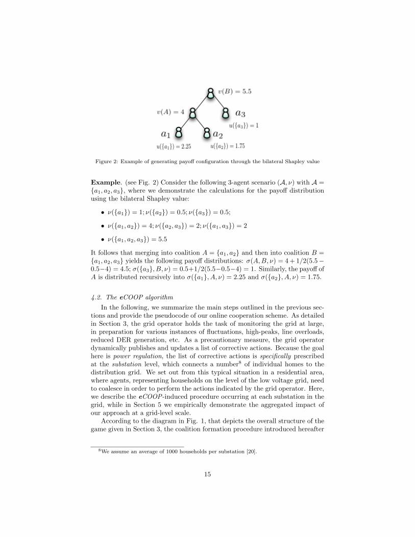
Figure 2: Example of generating payoff configuration through the bilateral Shapley value

Example. (see Fig. 2) Consider the following 3-agent scenario (A, ν) with A =a1, a2, a3, where we demonstrate the calculations for the payoff distributionusing the bilateral Shapley value:

• ν(a1) = 1; ν(a2) = 0.5; ν(a3) = 0.5;

• ν(a1, a2) = 4; ν(a2, a3) = 2; ν(a1, a3) = 2

• ν(a1, a2, a3) = 5.5

It follows that merging into coalition A = a1, a2 and then into coalition B =a1, a2, a3 yields the following payoff distributions: σ(A,B, ν) = 4 + 1/2(5.5−0.5−4) = 4.5; σ(a3, B, ν) = 0.5+1/2(5.5−0.5−4) = 1. Similarly, the payoff ofA is distributed recursively into σ(a1, A, ν) = 2.25 and σ(a2, A, ν) = 1.75.

4.2. The eCOOP algorithm

In the following, we summarize the main steps outlined in the previous sec-tions and provide the pseudocode of our online cooperation scheme. As detailedin Section 3, the grid operator holds the task of monitoring the grid at large,in preparation for various instances of fluctuations, high-peaks, line overloads,reduced DER generation, etc. As a precautionary measure, the grid operatordynamically publishes and updates a list of corrective actions. Because the goalhere is power regulation, the list of corrective actions is specifically prescribedat the substation level, which connects a number8 of individual homes to thedistribution grid. We set out from this typical situation in a residential area,where agents, representing households on the level of the low voltage grid, needto coalesce in order to perform the actions indicated by the grid operator. Here,we describe the eCOOP -induced procedure occurring at each substation in thegrid, while in Section 5 we empirically demonstrate the aggregated impact ofour approach at a grid-level scale.

According to the diagram in Fig. 1, that depicts the overall structure of thegame given in Section 3, the coalition formation procedure introduced hereafter

8We assume an average of 1000 households per substation [20].

15

corresponds to the second stage. It is important to point out that the BSV com-putation detailed in Section 4.1 is implicit to the implementation of the eCOOPalgorithm. That is, generating the coalition structure follows a bilateral coali-tion formation procedure, kickstarted from the set of singleton coalitions, havingeach agent reason about the expected utility of a potential coalition based on itspredictive model, constructed from previous encounters. During each iterationat least one new coalition is formed by merging of two coalitions, where theadded value of the coalition merger is to be distributed according to the bilat-eral Shapley value (Eq. 14). Moreover, by adhering to our protocol we enableconsumers to distributively converge to solutions that fulfil corrective actions,while also meeting the requirements of computing BSV-stable configurations.Given as input, for each consumer, the flexibility domain χ and the associateddiscomfort cost for each action within χ, this information is encapsulated bythe agent. Hereafter, the agent represents the consumer for the induced game,interacting with the other agents according to the eCOOP algorithm9.

The eCOOP algorithm is run by every agent in the system. The startingpoint for each agent is inspecting the global list of corrective actions providedby the grid operator, along with the associated probability of their occurrence.According to the user prescribed strategy, the agent selects a set of target eventsin EventQueue from CorrectiveActionsList (lines 3-4), which induce a set ofgoal-oriented cooperative games that are solved concurrently. Then, for eachtarget event, the agent determines the set of relevant actions according to Def-inition 6, inspecting for those that shift demand in line with the respectivetarget event. Next, for each target event the algorithm iteratively attempts toconstruct feasible coalitions starting from the initial set of singleton coalitions(line 6). A coalition represents an agreement between a group of agents for asuccessful resolution of a corrective action solicited by the grid operator. Basedon the information exchange (lines 32-43), each coalition computes internallythe expected utility of a bilateral merger with a potential coalition partner. Theevaluation of past collaborations are captured in the computation of the utility µof a coalition in a given coalition merger. Note that function µ is used through-out the algorithm to store and retrieve these values. Then, potential coalitionformations are simulated via mergers of subcoalitions by computing the coali-tion value as the mean of the expected utilities of the merging coalitions (line16). Following the assessment of potential coalition partners, for a designatedcandidate set where mergers provide an added reward (line 17), proposals areopportunistically advanced (lines 44-58).

Communication amongst agents assumes the use of time-outs by means ofwhich agents place upper bounds, specifying the amount of time allocated forreceiving a reply. In case no reply is received in due time, the particular agent issimply disregarded from being considered as a candidate for coalition formation.This simple request-response protocol is encapsulated by the Send/Receive pro-

9For instance by having the eCOOP functionality deployed inside the smart meter.

16

cedures, which specify respectively the sender and recipient agents (or coalitionleaders) and the message itself. Messages are routed to the destination agentand are placed in its message queue. The Receive procedure examines the mes-sage queue, retrieving null only if the timeout expires before a desired messagearrives and thus avoiding potential deadlocks during the inter-agent commu-nication. In short, communication with other agents is parallelized by addinga non-blocking agent behavior (thread) each time commnication with anotheragent commences (line 12). The same principle is applied for the inter-coalitioncommunication, where the coalition leader is responsible for aggregating the ex-pected utilities of a potential coalition merger based on the evaluations of themembers of its coalition (lines 37-38).

The simulation phase is followed by the actual coalition formation procedure,which is conducted in a distributed manner. Function MaxV alue is used toreturn the coalition with the highest expected utility from the Candidate set.If proposals are bilaterally accepted, such that a coalitions S1 and S2 bothevaluate the merger S = S1∪S2 as a preferable outcome compared to the currentconfiguration CSiter or to other possible mergers, then during the next iterationof the algorithm the new configuration CSiter+1 will substitute S1 and S2 withthe newly formed coalition S (line 25). Additionally, the Update function revisesthe current configuration based on notifications from other coalition leadersregarding mergers that has occurred at this stage. Also, in the event of a merger,the information is broadcasted not only to the other coalition leaders, but aswell, all coalition members are informed about the new configuration (line 51).The procedure terminates once the algorithm converges on a particular coalitionstructure, meaning that no new coalition mergers are bilaterally acceptable.Note, that the algorithm terminates after at most |A| rounds, since in eachnon-final round at least one coalition is formed.

Finally, once the corrective action has been performed by the coalition, thereward is distributed according to the BSV computation for that particularconfiguration (line 29), resulting in coalitions with stable payoff distributions.Specifically, once the event has elapsed, according to Equation 7, dependingon the compliance or non-compliance with the corrective action, a reward or apenalty is determined respectively. The amount is then distributed down thecoalitional tree based on the expected coalitional utilities µ (Definition 13) thatwere used in generating the tree structure. Additionally, agents update theirprobabilistic model (values of π) with the information inferred from the resultof the coalition formation procedure.

In the following we give the agent program of a leader agent ai in a coali-tion, where a leader is determined by lexicographic order. The algorithm startsfrom the set of singleton coalitions, thus initially each agent also plays the roleof coalition leader. Once an agent becomes part of a coalition and no longerfulfils the leader role, as a coalition member his role is confined to respondingrequests from the coalition leader. We focus on the abovementioned tasks per-formed by a leader agent by providing in Algorithm 1 the pseudocode of the

17

main thread, while Algorithm 2 and Algorithm 3 addresses respectively a num-ber of subroutines corresponding to the communication and negotiation phases.More elaborate ways to establish a coalition leader are beyond the scope of thispaper, however, in future work we intend to base this decision on additionalfactors such as the agents’ computational resources (i.e. the agent with thegreater computational power is preferred) or network properties (i.e. prioritizecommunication hubs).

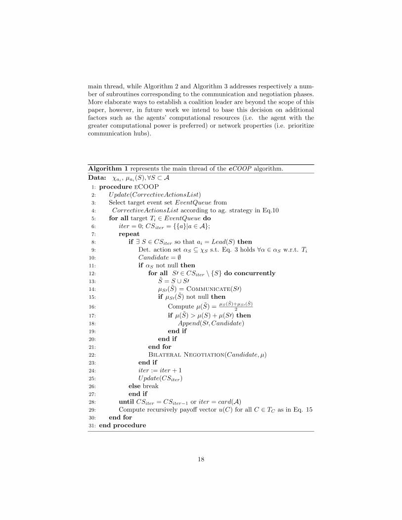
Algorithm 1 represents the main thread of the eCOOP algorithm.

Data: χai , µai(S),∀S ⊂ A1: procedure eCOOP2: Update(CorrectiveActionsList)3: Select target event set EventQueue from4: CorrectiveActionsList according to ag. strategy in Eq.105: for all target Ti ∈ EventQueue do6: iter = 0; CSiter = a|a ∈ A;7: repeat8: if ∃ S ∈ CSiter so that ai = Lead(S) then9: Det. action set αS ⊆ χS s.t. Eq. 3 holds ∀α ∈ αS w.r.t. Ti

10: Candidate = ∅11: if αS not null then12: for all S′ ∈ CSiter \ S do concurrently13: S = S ∪ S′14: µS′(S) = Communicate(S′)15: if µS′(S) not null then

16: Compute µ(S) = µS(S)+µS′(S)2

17: if µ(S) > µ(S) + µ(S′) then18: Append(S′, Candidate)19: end if20: end if21: end for22: Bilateral Negotiation(Candidate, µ)23: end if24: iter := iter + 125: Update(CSiter)26: else break27: end if28: until CSiter = CSiter−1 or iter = card(A)29: Compute recursively payoff vector u(C) for all C ∈ TC as in Eq. 1530: end for31: end procedure

18

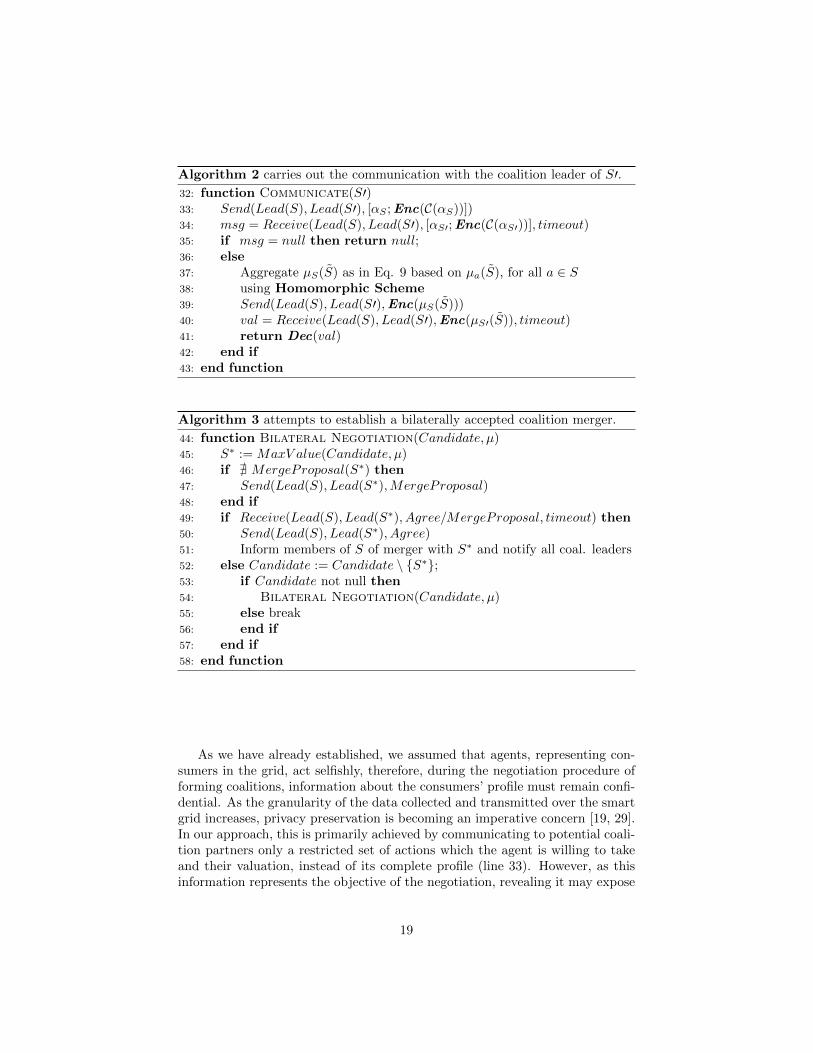
Algorithm 2 carries out the communication with the coalition leader of S′.32: function Communicate(S′)33: Send(Lead(S), Lead(S′), [αS ;Enc(C(αS))])34: msg = Receive(Lead(S), Lead(S′), [αS′;Enc(C(αS′))], timeout)35: if msg = null then return null;36: else37: Aggregate µS(S) as in Eq. 9 based on µa(S), for all a ∈ S38: using Homomorphic Scheme39: Send(Lead(S), Lead(S′),Enc(µS(S)))40: val = Receive(Lead(S), Lead(S′),Enc(µS′(S)), timeout)41: return Dec(val)42: end if43: end function

Algorithm 3 attempts to establish a bilaterally accepted coalition merger.

44: function Bilateral Negotiation(Candidate, µ)45: S∗ := MaxV alue(Candidate, µ)46: if @ MergeProposal(S∗) then47: Send(Lead(S), Lead(S∗),MergeProposal)48: end if49: if Receive(Lead(S), Lead(S∗), Agree/MergeProposal, timeout) then50: Send(Lead(S), Lead(S∗), Agree)51: Inform members of S of merger with S∗ and notify all coal. leaders52: else Candidate := Candidate \ S∗;53: if Candidate not null then54: Bilateral Negotiation(Candidate, µ)55: else break56: end if57: end if58: end function

As we have already established, we assumed that agents, representing con-sumers in the grid, act selfishly, therefore, during the negotiation procedure offorming coalitions, information about the consumers’ profile must remain confi-dential. As the granularity of the data collected and transmitted over the smartgrid increases, privacy preservation is becoming an imperative concern [19, 29].In our approach, this is primarily achieved by communicating to potential coali-tion partners only a restricted set of actions which the agent is willing to takeand their valuation, instead of its complete profile (line 33). However, as thisinformation represents the objective of the negotiation, revealing it may expose

19

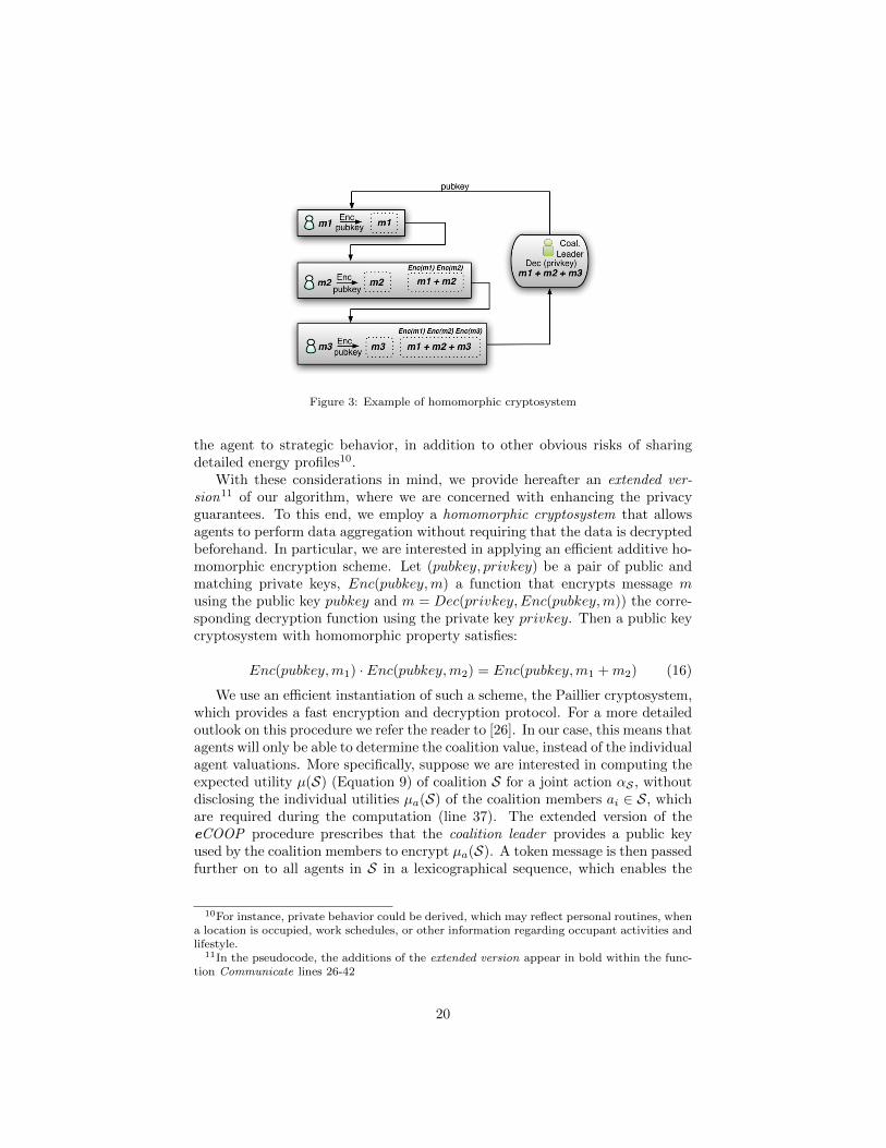
Figure 3: Example of homomorphic cryptosystem

the agent to strategic behavior, in addition to other obvious risks of sharingdetailed energy profiles10.

With these considerations in mind, we provide hereafter an extended ver-sion11 of our algorithm, where we are concerned with enhancing the privacyguarantees. To this end, we employ a homomorphic cryptosystem that allowsagents to perform data aggregation without requiring that the data is decryptedbeforehand. In particular, we are interested in applying an efficient additive ho-momorphic encryption scheme. Let (pubkey, privkey) be a pair of public andmatching private keys, Enc(pubkey,m) a function that encrypts message musing the public key pubkey and m = Dec(privkey,Enc(pubkey,m)) the corre-sponding decryption function using the private key privkey. Then a public keycryptosystem with homomorphic property satisfies:

Enc(pubkey,m1) · Enc(pubkey,m2) = Enc(pubkey,m1 +m2) (16)

We use an efficient instantiation of such a scheme, the Paillier cryptosystem,which provides a fast encryption and decryption protocol. For a more detailedoutlook on this procedure we refer the reader to [26]. In our case, this means thatagents will only be able to determine the coalition value, instead of the individualagent valuations. More specifically, suppose we are interested in computing theexpected utility µ(S) (Equation 9) of coalition S for a joint action αS , withoutdisclosing the individual utilities µa(S) of the coalition members ai ∈ S, whichare required during the computation (line 37). The extended version of theeCOOP procedure prescribes that the coalition leader provides a public keyused by the coalition members to encrypt µa(S). A token message is then passedfurther on to all agents in S in a lexicographical sequence, which enables the

10For instance, private behavior could be derived, which may reflect personal routines, whena location is occupied, work schedules, or other information regarding occupant activities andlifestyle.

11In the pseudocode, the additions of the extended version appear in bold within the func-tion Communicate lines 26-42

20

agents to construct iteratively the final result using the additive homomorphicscheme (see Fig. 3). Once all the agents have performed this action, the resultis sent to the coalition leader, who then decrypts it using the private key andmakes the result available to all agents. Based on the homomorphic property,only the aggregated result is decrypted, while intermediate agents aggregate theencrypted data during data forwarding, but cannot decrypt it. Importantly, thisapproach is guaranteed to achieve a security level of IND-CPA12, which is thehighest security level for homomorphic schemes [18].

The complexity of the proposed DCF (dynamic coalition formation) algo-rithm is given in the following propositions.

Proposition 1. The computation complexity of the algorithm is O(pn2m),where n = |A|, m = maxS∈CS|αS |, p = max|EventQueue|.

Proof. The number of iterations that the algorithm needs to cycle throughis bounded by a) the maximum number of events in the global queue O(p) (line5); b) the maximum number of coalition mergers that may occur O(n), whichcorresponds to the formation of the grand coalition (line 7); c) O(nm) the max-imum number of operations required in order to construct the list Candidate.Besides, the secure multi-party computation requires performing an encryp-tion for every sent message, while the destination agent is needed to add thecorresponding decryption. Hence, the overall complexity of the algorithm isO(p)O(n)O(nm) = O(pn2m).

Proposition 2. The communication complexity of the algorithm in thenumber of messages per agent is O(mnp).

Proof. During each run of the algorithm the number of messages sent by anagent is bounded by O(n)+O(m) for the case of coalition leaders, correspondingto inter-coalition negotiations and intra-coalition message passing respectively.Otherwise, a single message specifying µa is required to be sent to the coalitionleader for each iteration of the algorithm. In addition to this, due to the usage ofthe cryptographic layer, the coalition leader is also responsible for distributingthe public key to each agent, member of its coalition. Thus, given at most pnrounds of the algorithm, the overall number of messages sent by an agent isO(mnp).

5. Empirical Evaluation

In this section we provide an empirical evaluation of the coalition forma-tion mechanism introduced in Section 4. First, we explain the details of ourexperimental setup in Section 5.1. Then, in Section 5.2 we make several re-marks about our particular choice of a prediction model. Next, we analyse ourempirical results in Section 5.3.

12IND stands for indistinguishability and CPA for chosen plaintext attacks

21

5.1. Experimental Set-up

To evaluate the performance of our proposed algorithm, experiments wereconducted on real datasets obtained from the Australian Energy Market Oper-ator (AEMO)13. It is important to note that AEMO centrally coordinates thedispatch procedure via a real-time pricing scheme, onwards referred as RTP,by pooling the quantities of electricity required by consumers from availablegenerators. Essentially, RTP is a differential pricing scheme, where the cost perunit of electricity varies periodically throughout the day (i.e. peak consump-tion corresponds to price increases) and it is considered to be the most efficientdifferential price mechanism used for demand response [8]. Through the exper-iments we sought to study the emerging consumption patterns induced by theeCOOP scheme w.r.t the RTP approach14, for which archives of price and de-mand data for half-hourly intervals are available. The performance of eCOOP isdemonstrated under the assumption of an expected elasticity in demand, whichis modelled and simulated, given the lack of such data to document consumers’preference in providing power regulation services. We further assume that allmessages are processed correctly and all agents work properly.

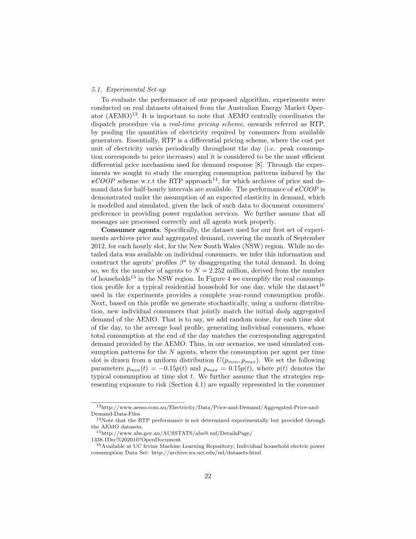
Consumer agents. Specifically, the dataset used for our first set of experi-ments archives price and aggregated demand, covering the month of September2012, for each hourly slot, for the New South Wales (NSW) region. While no de-tailed data was available on individual consumers, we infer this information andconstruct the agents’ profiles βa by disaggregating the total demand. In doingso, we fix the number of agents to N = 2.252 million, derived from the numberof households15 in the NSW region. In Figure 4 we exemplify the real consump-tion profile for a typical residential household for one day, while the dataset16

used in the experiments provides a complete year-round consumption profile.Next, based on this profile we generate stochastically, using a uniform distribu-tion, new individual consumers that jointly match the initial daily aggregateddemand of the AEMO. That is to say, we add random noise, for each time slotof the day, to the average load profile, generating individual consumers, whosetotal consumption at the end of the day matches the corresponding aggregateddemand provided by the AEMO. Thus, in our scenarios, we used simulated con-sumption patterns for the N agents, where the consumption per agent per timeslot is drawn from a uniform distribution U(pmin, pmax). We set the followingparameters pmin(t) = −0.15p(t) and pmax = 0.15p(t), where p(t) denotes thetypical consumption at time slot t. We further assume that the strategies rep-resenting exposure to risk (Section 4.1) are equally represented in the consumer

13http://www.aemo.com.au/Electricity/Data/Price-and-Demand/Aggregated-Price-and-Demand-Data-Files

14Note that the RTP performance is not determined experimentally but provided throughthe AEMO datasets.

15http://www.abs.gov.au/AUSSTATS/abs@.nsf/DetailsPage/1338.1Dec%202010?OpenDocument

16Available at UC Irvine Machine Learning Repository; Individual household electric powerconsumption Data Set: http://archive.ics.uci.edu/ml/datasets.html

22

Figure 4: Example of a daily load curve for an individual household

population and that the extent to which consumers are willing to rescheduledemand by shifting loads is constrained to Υ = 25% of the total consump-tion, denoting their elasticity of demand as recent reports suggest [9, 17]. Itis estimated that shiftable loads (i.e. washing machines, dish washers) accounton average 25% of the electricity usage of a household, the remainder beinglargely due to entertainment and lightning purposes. For associating shiftableloads with consumer profiles we generate loads with a duration of one time-slot,which are distributed uniformly over the set of time slots T = 1, . . . , 24, tomatch the given elasticity of demand. The number of time slots to which eachload can be shifted is bounded to ∆ ∈ [−5, 5], while the power ratings of theseloads are uniformly distributed in the set r ∈ 1kW, 2kW, 3kW. Hence, theflexibility domain of an agent consists of the set of possible actions, where anaction links a shiftable load l to a potential deferment ∆ (Def. 4).

Grid operator. A corrective action prescribes that demand needs to beshifted from a time slot ti to another time slot tj . Whenever the grid opera-tor determines that the average daily consumption is expected to be exceededby more than 5%, a corrective action is triggered, requesting that this excessdemand is shifted to the following time-slot with a lower than average consump-tion. Corrective actions are made available to subsets of N , of a fixed sized,which is set to 1000 agents (hence preserving the local character of power reg-ulation at the substation level). Additionally, in order to give a measure ofrobustness, we factored into our simulation random variations in the power sup-ply, accounting for fluctuations from renewable resources, which are estimatedto cover about 13% of the total generation [9]. The mean absolute percentagedeviation (MAPD) is bounded to 20%. Such instances may also represent thecause for requesting corrective actions in case the abovementioned triggeringcondition is met. Also, we consider without loss of generality that coalitionsperform joint actions successfully with a 90% probability rate, in accordanceto recent consumer behavior surveys on customer acceptance retention and re-

23

sponse to time based electricity tariffs [34]. This optimistic scenario assumes infact that 9 out of 10 coalitions are compliant with their respective corrective ac-tion requests. Given the previously mentioned fixed maximum size of coalitions,it follows that the performance improvement is linear with this rate.

In specifying a corrective action request, the grid operator ought to providethe associated reward and penalty functions (Def. 2). For our scenario, the re-ward is based on the assumption that the approximate cost otherwise incurredby deploying expensive power plants is instead distributed to consumers willingto reduce demand (hence achieving lower emissions). Evidently, in a real sce-nario, the grid operator may choose to commit only a fraction of this amountfor incentivising consumers. We use the following reward function in Equation17, supposing that the desired amount of demand to be shifted is q∗ and setθ = 0.1 (cents). It is important to point out that besides complying with theproperties of Eq. 4, quadratic functions are commonly used to capture the costof electricity supply (see [28]). We further consider P(q) = f(q).

R(q) =

f(q) = θq2 if q < q∗

0 if q ≥ q∗ (17)

5.2. Predictive Model

The aspects of building an estimation model regarding potential coalitionpartners, based on previous encounters, as well as the agent’s own estimateduser behavior, have been addressed in Section 4.1. In our experiments, weapproach both aspects in a unified manner by including sources of uncertaintyin the form of random, uncontrollable variables with probability distributions,that each agent attempts to learn in an online fashion. Recall that for eachagent a ∈ A there corresponds a set of (deferrable) loads La. Essentially, thegoal is to learn for a given action αlj , that shifts a load lj , the likelihood thatthe shift occurs to a particular timeslot k. Suppose now that agent a wantsto determine the likelihood for each of the actions that constitute its flexibilityset χa. Let R = r1, . . . , r|χa| denote the set of random variables modellingfuture, uncontrollable events and D = D1, . . . , Dq, a set of domains for therandom variables such that ri takes values in Di = T . Let σ : R → χa be adistribution function of random variables to the agent’s actions. Agent a learnsP = π1, . . . , π|χa|, which is a set of probability distributions for the randomvariables, where each distribution πi : Di → [0, 1] defines the probability law forrandom variable ri, such that the values of πi sum up to 1.

Also, there is uncertainty regarding the expected behavior of potential coali-tion partners, which in turn need to conform to their respective user demandsin a timely fashion. Similarly, agent a tracks past encounters with other agentsand builds a probability set Pi for each agent ai. Consequently, we exploit therepeated game structure of the problem to learn a prediction model regardingfuture interactions and thus infer potential synergies between agents.

24

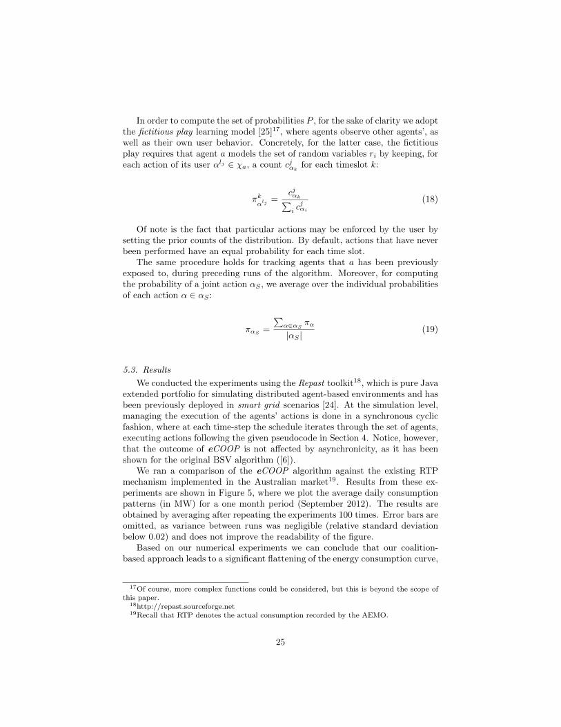
In order to compute the set of probabilities P , for the sake of clarity we adoptthe fictitious play learning model [25]17, where agents observe other agents’, aswell as their own user behavior. Concretely, for the latter case, the fictitiousplay requires that agent a models the set of random variables ri by keeping, foreach action of its user αlj ∈ χa, a count cjαk

for each timeslot k:

πkαlj

=cjαk∑icjαi

(18)

Of note is the fact that particular actions may be enforced by the user bysetting the prior counts of the distribution. By default, actions that have neverbeen performed have an equal probability for each time slot.

The same procedure holds for tracking agents that a has been previouslyexposed to, during preceding runs of the algorithm. Moreover, for computingthe probability of a joint action αS , we average over the individual probabilitiesof each action α ∈ αS :

παS=

∑α∈αS

πα

|αS |(19)

5.3. Results

We conducted the experiments using the Repast toolkit18, which is pure Javaextended portfolio for simulating distributed agent-based environments and hasbeen previously deployed in smart grid scenarios [24]. At the simulation level,managing the execution of the agents’ actions is done in a synchronous cyclicfashion, where at each time-step the schedule iterates through the set of agents,executing actions following the given pseudocode in Section 4. Notice, however,that the outcome of eCOOP is not affected by asynchronicity, as it has beenshown for the original BSV algorithm ([6]).

We ran a comparison of the eCOOP algorithm against the existing RTPmechanism implemented in the Australian market19. Results from these ex-periments are shown in Figure 5, where we plot the average daily consumptionpatterns (in MW) for a one month period (September 2012). The results areobtained by averaging after repeating the experiments 100 times. Error bars areomitted, as variance between runs was negligible (relative standard deviationbelow 0.02) and does not improve the readability of the figure.

Based on our numerical experiments we can conclude that our coalition-based approach leads to a significant flattening of the energy consumption curve,

17Of course, more complex functions could be considered, but this is beyond the scope ofthis paper.

18http://repast.sourceforge.net19Recall that RTP denotes the actual consumption recorded by the AEMO.

25

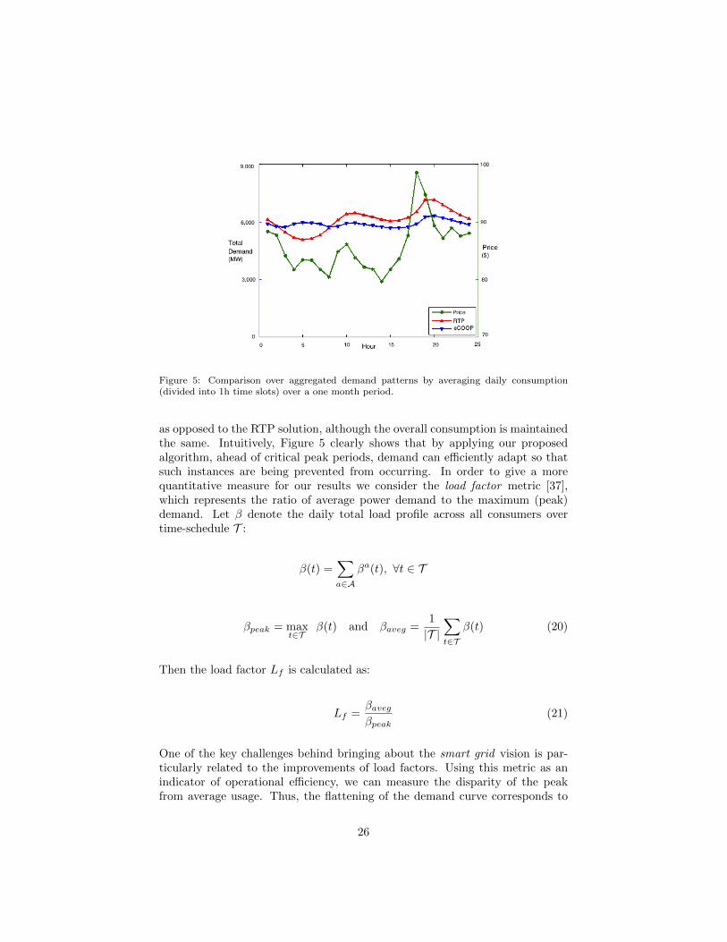
Figure 5: Comparison over aggregated demand patterns by averaging daily consumption(divided into 1h time slots) over a one month period.

as opposed to the RTP solution, although the overall consumption is maintainedthe same. Intuitively, Figure 5 clearly shows that by applying our proposedalgorithm, ahead of critical peak periods, demand can efficiently adapt so thatsuch instances are being prevented from occurring. In order to give a morequantitative measure for our results we consider the load factor metric [37],which represents the ratio of average power demand to the maximum (peak)demand. Let β denote the daily total load profile across all consumers overtime-schedule T :

β(t) =∑a∈A

βa(t), ∀t ∈ T

βpeak = maxt∈T

β(t) and βaveg =1

|T |∑t∈T

β(t) (20)

Then the load factor Lf is calculated as:

Lf =βavegβpeak

(21)

One of the key challenges behind bringing about the smart grid vision is par-ticularly related to the improvements of load factors. Using this metric as anindicator of operational efficiency, we can measure the disparity of the peakfrom average usage. Thus, the flattening of the demand curve corresponds to

26

an increase of the load factor toward unity. For the one-month interval we haveconsidered in our experiments, our approach produces a 14% increase of the loadfactor from 0.77 for the RTP scheme to 0.91 when applying the eCOOP algo-rithm. Through our approach, we aim that the aggregated load is more evenlydistributed across the time schedule T . In contrast, traditional approaches, thataim to nudge user consumption using price signals broadcasted to all, in effect,attempt that each user individually achieves a more balanced load, which neednot necessarily be the case for eCOOP. Here, we move the focus from the bilat-eral interaction between the grid operator and consumers, to a setting where weenable direct interactions between consumers, incentivized by the grid operator,such that their coordinated effort achieves a improved Lf value.

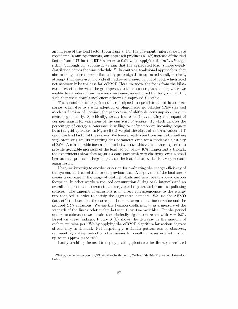
The second set of experiments are designed to speculate about future sce-narios, when due to a wide adoption of plug-in electric vehicles (PEV) as wellas electrification of heating, the proportion of shiftable consumption may in-crease significantly. Specifically, we are interested in evaluating the impact ofour mechanism for variations of the elasticity of demand Υ, which denotes thepercentage of energy a consumer is willing to defer upon an incoming requestfrom the grid operator. In Figure 6 (a) we plot the effect of different values of Υupon the load factor of the system. We have already seen from our initial settingvery promising results regarding this parameter even for a moderate elasticityof 25%. A considerable increase in elasticity above this value is thus expected toprovide negligible increases of the load factor, below 10%. Importantly though,the experiments show that against a consumer with zero elasticity, even a smallincrease can produce a large impact on the load factor, which is a very encour-aging result.

Next, we investigate another criterion for evaluating the energy efficiency ofthe system, in close relation to the previous case. A high value of the load factormeans a decrease in the usage of peaking plants and as a result, a lower carbonfootprint. In other words, a reduced consumption during peak intervals and anoverall flatter demand means that energy can be generated from less pollutingsources. The amount of emissions is in direct correspondence to the energymix required in order to satisfy the aggregated demand. We use the AEMOdataset20 to determine the correspondence between a load factor value and theinduced CO2 emissions. We use the Pearson coefficient, r, as a measure of thestrength of the linear relationship between these two variables. For the periodunder consideration we obtain a statistically significant result with r = 0.81.Based on these findings, Figure 6 (b) shows the decrease in the amount ofcarbon emission per kWh by applying the eCOOP algorithm for various degreesof elasticity in demand. Not surprisingly, a similar pattern can be observed,representing a steep reduction of emissions for small increases in elasticity forup to an approximate 20%.

Lastly, avoiding the need to deploy peaking plants can be directly translated

20http://www.aemo.com.au/Electricity/Settlements/Carbon-Dioxide-Equivalent-Intensity-Index

27

Figure 6: Average evolution of (a) load factor, (b) carbon emissions and (c) percetage savingsfor different degrees of elasticity of demand

28

Figure 7: Simulation results for year-round load factor comparison averaged monthly

into consumer savings. In Figure 5 we have also represented the evolution ofreal-time pricing according to the given aggregated demand, as provided by theAEMO dataset. Observably, off-peak intervals are correlated with lower prices,while higher prices correspond to peak periods. As we have seen, applying ouralgorithm produces on aggregate a modified consumption pattern. We now de-termine the average cost savings perceived by consumers, assuming that the costof electricity (per kWh) is given by the total demand in the system accordingto the RTP pricing in our dataset. We plot the results in Figure 6 (c), where wegive an estimation of percent savings incurred by consumers during the time slotwith the highest consumption during the day, for varying degrees of elasticity.This is again an encouraging result, showing an approximate 30% reduction ofkWh cost in return for an elasticity of 20%. Further flexibility in consumptioncan lead to a reduction of up to 40%.

Finally, we provide conclusive results for the performance of our algorithm,demonstrating how eCOOP outperforms the existing RTP scheme, evaluatedover an extended year-round scenario (Sept. 2012 - Sept. 2013). It is impor-tant to note that consumption patterns vary throughout the year. Specifically,winter and summer months are known to exhibit increased high-peak intervalsdue to an intense usage of electricity. We started our experiments investigatingan average consumption month. For generality, we now give in Figure 7 theyear-round results based on the load factor computation for the two approachesunder consideration. It is interesting to observe that RTP produces differentoutcomes depending on the particular period of the year, highly correlated tothe expected consumption usage. For instance, on the one hand, the lowestefficiency is observed during January with a load factor value of 0.6 and on theother hand, April and November represent the highest efficiency months. Incontrast, eCOOP consistently manages to attain a higher efficiency of an ap-proximately 0.9 load factor value, invariantly of the period under consideration,

29

while producing an average 17% improvement.

6. Conclusions

In this paper we are interested in a mechanism that can cope with an in-creasing amount of intermittent energy generated via renewable resources. Weintroduced the eCOOP agent-based algorithm, where look-ahead coalitional ne-gotiations are run within minimal information environments in order to addressthe dynamism and uncertainty of the energy system. Furthermore, our protocolprovides for computing an efficient payoff allocation scheme that guarantees sta-ble coalitions, while the extended version offers strong guarantees for satisfyingprivacy-preservation of sensitive data. We have also provided an empirical eval-uation of our approach based on real datasets and have shown the advantagesof using it in terms of increased grid efficiency.

It is important to point out that, by design, the intervention of the gridoperator addresses explicitly the shifting actions that consumer need to performin order to collect the reward. In contrast to traditional pricing schemes, thisallows us to impose the necessary constraints such that by removing peakswe are not replacing them by new ones, which is also known as the herdingeffect. Moreover, the design of the reward function allows us to transfer theresponsibility of determining the reliability of the agents to carry out correctiveactions, from the grid operator to the agents themselves.

In this work we have used a standard approach for computing the predictionmodel, namely fictitious play. In future work we plan to look into more complexmodels and assess their performance. Also, providing an extensive study on theimpact of the communication infrastructure is another interesting future line ofwork, which does not make the scope of this paper, hence we do not involvewith it deeply. We hypothesize that a more efficient way to determine coalitionleaders would be to account for the agents’ communication and computationalresources. Additionally, we assume that eCOOP is not affected by any dataloss or noise, while messages are sent, received and processed exactly in theorder prescribed in the pseudocode. However, enhancing the protocol withsynchronization procedures initiated by coalition leaders, in order to check forcorrect message passing along the execution of the algorithm, is one way thatcould guarantee robustness.

Moreover, we are interested to evaluate our model in scenarios where con-sumers are not only willing to shift loads to different time intervals given mon-etary incentives, but may additionally be considering to reduce their total con-sumption given that a certain revenue could be attained. Expectedly, this oughtto further flatten demand and thus, increase the overall efficiency of the grid,especially during periods when generation from renewables is highly fluctuat-ing. Unfortunately, specifying these sorts of parameters, such as the thresholdin revenue to which consumers may react and the extent to which their con-sumption behavior may be altered, remains an open question. With more pilotprograms led by utility companies surfacing in this area, we expect that in the

30

future more of this type of data will become available. For the same consider-ations, given the lack of data required to quantitatively assess how consumerswould price potential shifting actions in a realistic setting, in this work, we feelmore confident in presenting the result with respect to the elasticity in demandof consumers and only provide an indication of maximum user savings, basedon the electricity price decrease corresponding to the levels of demand. In thisregard, we aim to dwell on this type of evaluation more deeply in future worksubject to the availability of relevant data.

Acknowledgements. This work has been partially supported by the Span-ish Ministry of Economy and Competitiveness through grants CSD2007-00022(”Agreement Technologies”, CONSOLIDER-INGENIO2010), TIN2012-36586-C03-02 (”iHAS”) and TIN2015-65515-C4-4-R (SURF) as well as by the by theAutonomous Region of Madrid through grant P2013/ICE-3019 (”MOSI-AGIL-CM”, co-funded by EU Structural Funds FSE and FEDER”) and by the Knowl-edge Foundation through the Internet of Things and People research profile.

References

[1] Blankenburg, B. and Klusch, M. (2005). BSCA-P: Privacy preserving coali-tion formation. In Eymann, T., Klugl, F., Lamersdorf, W., Klusch, M., andHuhns, M., editors, Multiagent System Technologies, volume 3550 of LectureNotes in Computer Science, pages 47–58. Springer Berlin Heidelberg.

[2] Chalkiadakis, G., Robu, V., Kota, R., Rogers, A., and Jennings, N. R.(2011). Cooperatives of distributed energy resources for efficient virtual powerplants. In Proc. of The 10th International Conference on Autonomous Agentsand Multiagent Systems AAMAS, pages 787–794.

[3] Chris, H. (2008). Electricity markets: Pricing, structures & economics.European Journal of Control, 14(4).

[4] Contreras, J., Klusch, M., Vielhak, T., Yen, J., and Wu, F. (1999). Multi-agent coalition formation in transmission planning bilateral Shapley valueand kernel approaches. In Proc. of the 13th Power Systems ComputationConference, pages 777–787.

[5] Contreras, J., Klusch, M., and Yen, J. (1998). Multiagent coalition forma-tion in power transmission planning: a bilateral Shapley value approach. InProc. of the 4th International Conference on Artificial Intelligence PlanningSystems, pages 19–26.

[6] Contreras, J., Wu, F., Klusch, M., and Shehory, O. (1997). Coalition for-mation in a power transmission planning environment. In Proc. of 2nd Intl.Conference on Practical Applications of Multi-Agent Systems, PAAM, pages21–23.

31

[7] Costa, L., Bourry, F., Juban, J., and Kariniotakis, G. (2008). Managementof energy storage coordinated with wind power under electricity market con-ditions. In Probabilistic Methods Applied to Power Systems, 2008. PMAPS’08. Proceedings of the 10th International Conference on, pages 1–8.

[8] Edward J. Bloustein School of Planning and Public Pol-icy (2006). Assessment of customer response to real timepricing. Technical report. http://ceeep.rutgers.edu/wp-content/uploads/2013/11/customerresponse.pdf.

[9] European SmartGrids Technology Platform (2006). Vision and strategyfor european electricity networks of the future. Technical report, EuropeanCommission. http://ec.europa.eu/research/energy/pdf/smartgrids en.pdf.

[10] Hammerstrom, D. J., Brous, J., Chassin, D. P., Horst, G. R., Kajfasz, R.,Michie, P., Oliver, T. V., Carlon, T. A., Eustis, C., and Jarvegren, O. M.(2007). Pacific northwest gridwise testbed demonstration projects; part II.grid friendly appliance project. Technical Report PNNL-17079, Pacific North-west National Laboratory.

[11] Humeau, S. F. R. J., Wijaya, T. K., Vasirani, M., and Aberer, K. (2013).Electricity Load Forecasting for Residential Customers: Exploiting Aggrega-tion and Correlation between Households. In Sustainable Internet and ICTfor Sustainability (SustainIT), pages 1–6.

[12] Infield, D., Short, J., Home, C., and Freris, L. (2007). Potential for domesticdynamic demand-side management in the UK. In Power Engineering SocietyGeneral Meeting, 2007. IEEE, pages 1 –6.

[13] Kamboj, S., Kempton, W., and Decker, K. S. (2011). Deploying powergrid-integrated electric vehicles as a multi-agent system. Proceedings of theTenth International Joint Conference on Autonomous Agents and MultiagentSystems (AAMAS 2011), pages 13–20.

[14] Ketchpel, S. P. (1993). Coalition formation among autonomous agents. InProc. of Modelling Autonomous Agents in a Multi-Agent World (MAAMAW),pages 73–88.

[15] Klusch, M. (1998). Kooperative Informationsagenten im Internet. Dr Ko-vacz Verlag. ISBN: 3-86064-746-6.

[16] Klusch, M. and Gerber, A. (2002). Dynamic coalition formation amongrational agents. IEEE Intelligent Systems, 17:42–47.

[17] MacKay, D. (2009). Sustainable Energy without the hot air. UIT Cam-bridge.

[18] Mao, W. (2003). Modern Cryptography: Theory and Practice. PrenticeHall Professional Technical Reference.

32

[19] McDaniel, P. and McLaughlin, S. (2009). Security and privacy challengesin the smart grid. Security Privacy, IEEE, 7(3):75 –77.

[20] McDonald, J., Wojszczyk, B., Flynn, B., and Voloh, I. (2013). Distributionsystems, substations, and integration of distributed generation. In Begovic,M. M., editor, Electrical Transmission Systems and Smart Grids, pages 7–68.Springer New York.

[21] Mihailescu, R.-C., Vasirani, M., and Ossowski, S. (2011). Agame-theoretic coordination framework for energy-efficient demand-side management in the smart grid. In Proceedings of theNinth European Workshop on Multi-agent Systems (EUMAS).http://webshare.mah.se/af4299/Files/EUMAS11/paper.pdf.

[22] Newsham, G. R. and Bowker, B. G. (2010). The effect of utility time-varying pricing and load control strategies on residential summer peak elec-tricity use: A review. Energy Policy, 38(7):3289 – 3296.

[23] Ng, K.-H. and Sheble, G. (1998). Direct load control-a profit-based loadmanagement using linear programming. Power Systems, IEEE Transactionson, 13(2):688–694.

[24] North, M. J., Conzelmann, V., Koritarov, C., Macal, C., Thimmapuram,P., and Veselka, T. (2002). E-Laboratories: agent-based modeling of electric-ity markets. In American Power Conference.

[25] Osborne, M. and Rubinstein, A. (1994). A Course in Game Theory. MITPress.

[26] Paillier, P. and Pointcheval, D. (1999). Efficient public-key cryptosystemsprovably secure against active adversaries. In ASIACRYPT, pages 165–179.

[27] Ramchurn, S., Vytelingum, P., Rogers, A., and Jennings, N. R. (2012).Putting the ”smarts” into the smart grid: A grand challenge for artificialintelligence. Communications of the ACM, 55(4):86–97.

[28] Ramchurn, S. D., Vytelingum, P., Rogers, A., and Jennings, N. R. (2011).Agent-based control for decentralised demand side management in the smartgrid. In Proc. of The 10th International Conference on Autonomous Agentsand Multiagent Systems AAMAS, pages 5–12.

[29] Rashvand, H., Salah, K., Calero, J., and Harn, L. (2010). Distributed secu-rity for multi-agent systems - review and applications. Information Security,IET, 4(4):188 –201.

[30] Salehfar, H., Noll, P. J., LaMeres, B., Nehrir, M., and Gerez, V. (1999).Fuzzy logic-based direct load control of residential electric water heaters andair conditioners recognizing customer preferences in a deregulated environ-ment. In Power Engineering Society Summer Meeting, 1999. IEEE, volume 2,pages 1055–1060 vol.2.

33

[31] Shapley, L. S. (1953). A value for n-person games. Contributions to thetheory of games, 2:307–317.

[32] Strbac, G. (2008). Demand side management: Benefits and challenges.Energy Policy, 36(12):4419–4426.

[33] Tompros, S. L., Mouratidis, N. P., Draaijer, M., Foglar, A., and Hras-nica, H. (2009). Enabling applicability of energy saving applications on theappliances of the home environment. IEEE Network, 23(6):8–16.

[34] U.S. Department of Energy (2015). Interim report on im-pacts from the consumer behavior studies. Technical re-port. http://energy.gov/sites/prod/files/2015/06/f24/ARRA-CBS interim program impact report June2015.pdf.

[35] Vasirani, M., Ossowski, S., Kota, R., Cavalcante, R. L. G., and Jennings,N. R. (2011). Using coalitions of wind generators and electric vehicles foreffective energy market participation. In Proc. of the 10th InternationalConference on Autonomous Agents and Multiagent Systems, AAMAS, pages1099–1100.

[36] Vytelingum, P., Voice, T. D., Ramchurn, S. D., Rogers, A., and Jennings,N. R. (2010). Agent-based micro-strorage management for the smart grid. InProc. of the 8th International Conerence on Autonomous Agents And Multi-Agent Systems, AAMAS, pages 39–46.

[37] Weedy, B. M. and Cory, B. J. (2004). Electric Power Systems. John WileySons. 4th edition.

[38] Wei, D.-C. and Chen, N. (1995). Air conditioner direct load control bymulti-pass dynamic programming. Power Systems, IEEE Transactions on,10(1):307–313.

[39] Yang, H.-T. and Huang, K.-Y. (1999). Direct load control using fuzzydynamic programming. Generation, Transmission and Distribution, IEEProceedings-, 146(3):294–300.

34