Embed Size (px)
Citation preview
1
Coastal Information Team
Ecosystem Spatial AnalysesApril 2, 2004
OVERVIEWOVERVIEW•Scope, Purpose, Process
•Conservation Targets
•Conservation Goals
•Impacts
•Spatial Analysis
•Options and Scenarios
•Results
•Summary

2
OVERVIEWOVERVIEW•Scope, Purpose, Process
•Conservation Targets
•Conservation Goals
•Impacts
•Spatial Analysis
•Options and Scenarios
•Results
•Summary
ESA terms of Reference
• Identify areas of biodiversity significance and set conservationpriorities for the CIT study area
• Use credible, transparent and repeatable planning techniques grounded in the principles of conservation biology
• Use explicit goals that can be translated into quantitative, operational benchmarks
• Create robust end products for communicating our results to the CIT, planning tables, and other appropriate stakeholders
• Integrate results into an ecologically based and shared framework for taking action and measuring results.

3
ESA Team
• Conservation Science Inc.• The Nature Conservancy of Canada• The Nature Conservancy (U.S.)• Living Oceans Society• Round River Conservation Studies • Min. of Sustainable Resource Management• Min. of Water, Air and Land Protection
4
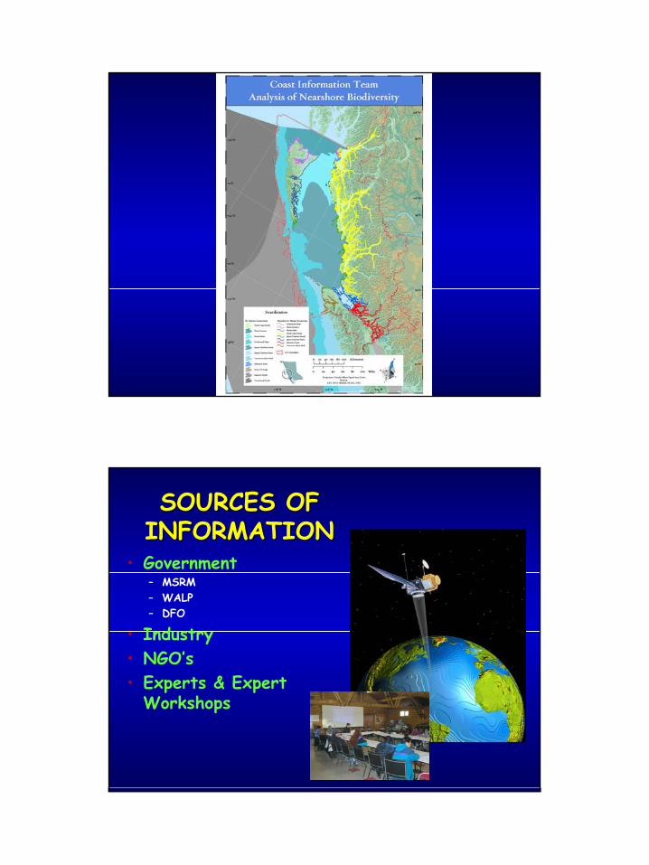
SOURCES OFSOURCES OFINFORMATIONINFORMATION
• Government– MSRM– WALP– DFO
• Industry• NGO’s• Experts & Expert
Workshops
5
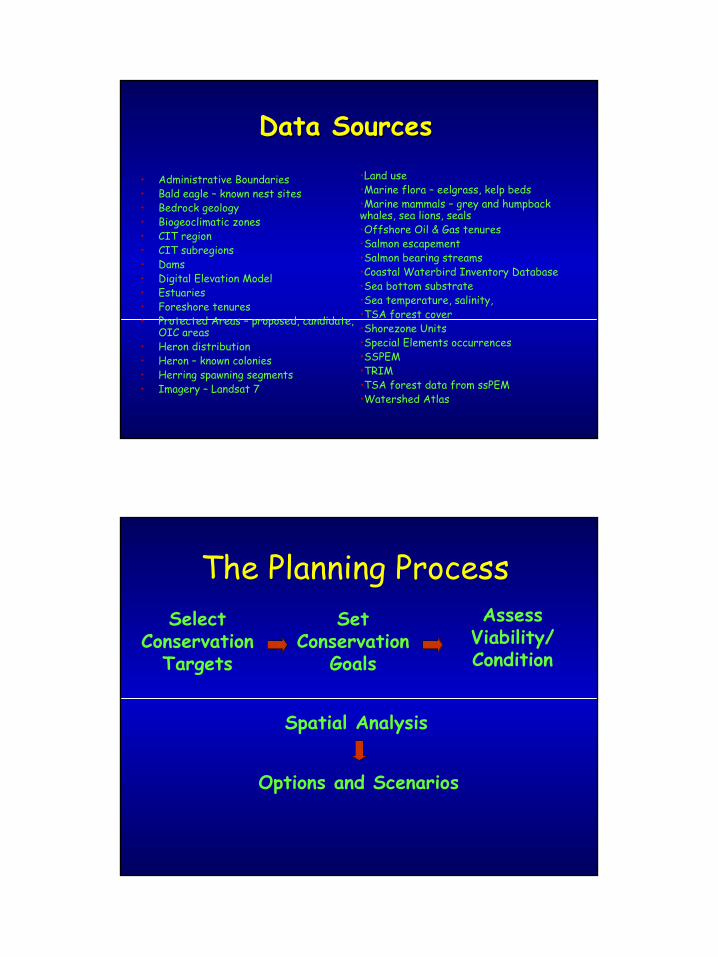
Data SourcesData Sources
• Administrative Boundaries• Bald eagle – known nest sites• Bedrock geology• Biogeoclimatic zones• CIT region• CIT subregions• Dams• Digital Elevation Model• Estuaries• Foreshore tenures• Protected Areas – proposed, candidate,
OIC areas• Heron distribution• Heron – known colonies• Herring spawning segments• Imagery – Landsat 7
•Land use•Marine flora – eelgrass, kelp beds•Marine mammals – grey and humpback whales, sea lions, seals•Offshore Oil & Gas tenures•Salmon escapement•Salmon bearing streams•Coastal Waterbird Inventory Database•Sea bottom substrate•Sea temperature, salinity,•TSA forest cover•Shorezone Units•Special Elements occurrences•SSPEM•TRIM•TSA forest data from ssPEM•Watershed Atlas
The Planning ProcessSelect
Conservation Targets
Set Conservation
Goals
Assess Viability/ Condition
Spatial Analysis
Options and Scenarios

6
OVERVIEWOVERVIEW•Scope, Purpose, Process
•Conservation Targets
•Conservation Goals
•Impacts
•Spatial Analysis
•Options and Scenarios
•Results
•Summary
Conservation TargetsConservation Targets
–Terrestrial
–Freshwater
–Marine Nearshore
–Marine Deepwater
•Special Elements
•Focal Species
•Ecosystem Representation
7
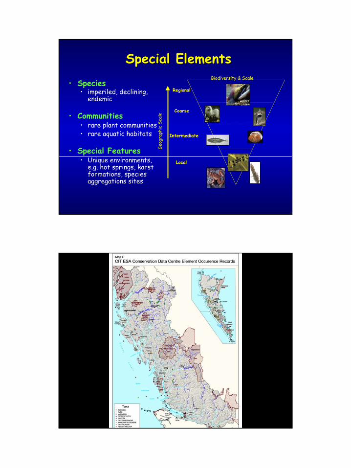
• Species• imperiled, declining,
endemic
• Communities• rare plant communities• rare aquatic habitats
• Special Features• Unique environments,
e.g. hot springs, karst formations, species aggregations sites
Special ElementsSpecial ElementsBiodiversity & Scale
Geog
raph
ic S
cale
Local
Intermediate
Coarse
Regional

8
Seabird Colonies
Population Density and Marine Usage
CIT Marine AnalysisCIT Marine Analysis
D. Gunn
British ColumbiaBritish ColumbiaHerring Spawn
Keystone Species
CIT Marine AnalysisCIT Marine Analysis

9
Focal SpeciesFocal Species
• Wide-ranging• Low densities, large habitat
requirements or key habitat attributes
• Habitat Suitability Modeled
Terrestrial Focal SpeciesTerrestrial Focal Species
• Grizzly Bear• Black Bear• Mountain Goat• Black-Tailed Deer• Northern Goshawk

10

11
12
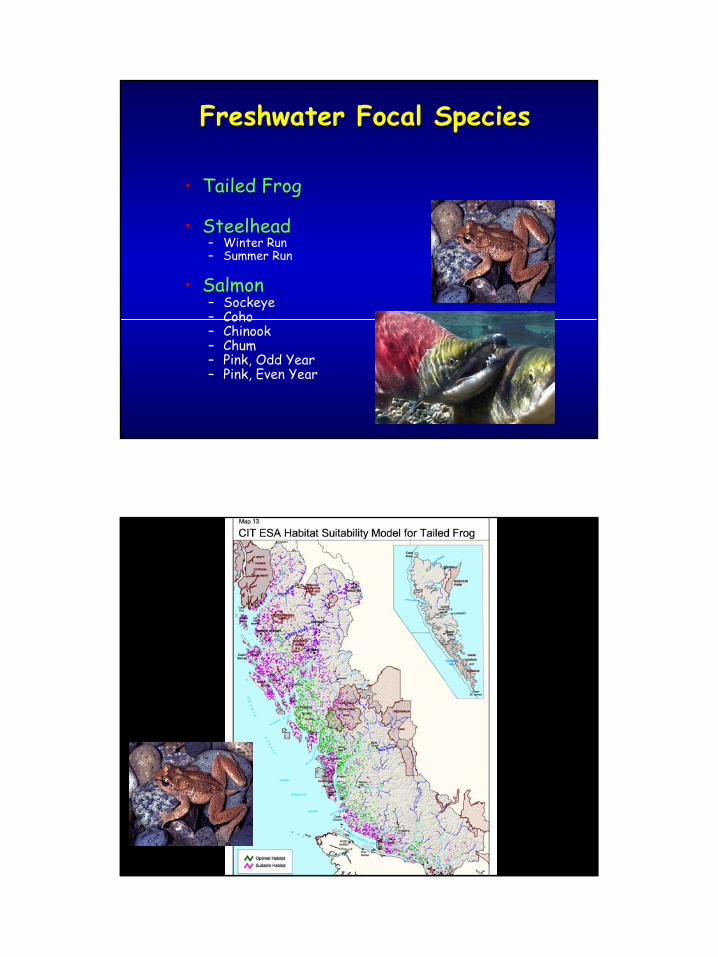
Freshwater Focal SpeciesFreshwater Focal Species
• Tailed Frog
• Steelhead– Winter Run– Summer Run
• Salmon– Sockeye– Coho– Chinook– Chum– Pink, Odd Year– Pink, Even Year

13
•DFO salmon escapement data for over 2000 salmon runs sampled for over 50 years.
•Run / population viability was assessed using trend analysis on DFO escapement data as well as expert review
•Biomass
•Salmon stock areas were defined for each salmon species based on expert review and known escapement data
Salmon and SteelheadSalmon and Steelhead
Chinook EscapementsLower Skeena River
14
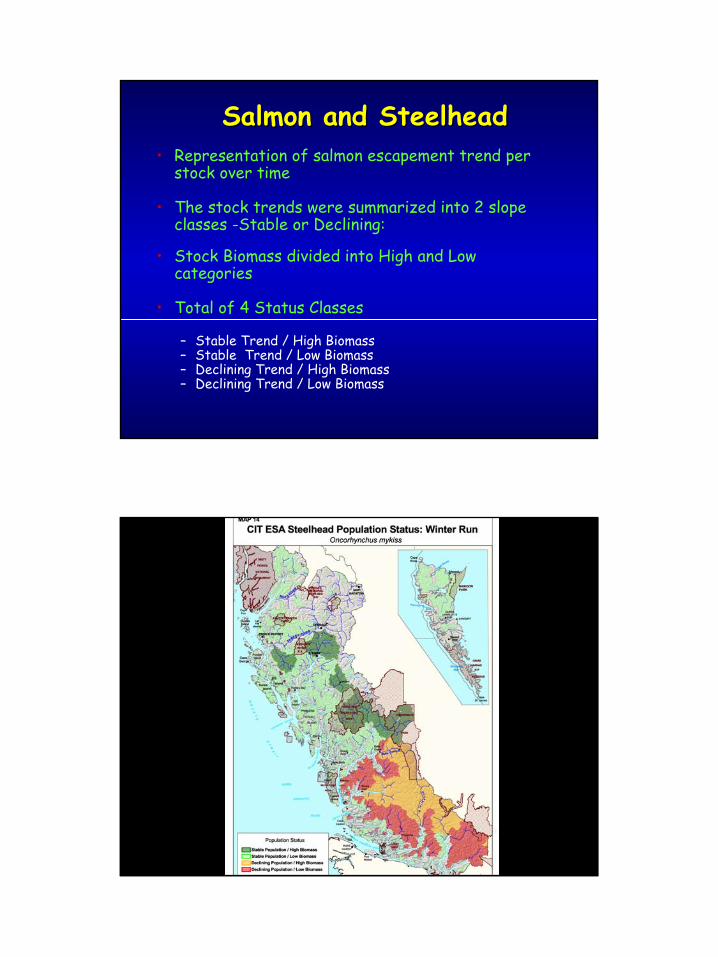
Salmon and SteelheadSalmon and Steelhead• Representation of salmon escapement trend per
stock over time
• The stock trends were summarized into 2 slope classes -Stable or Declining:
• Stock Biomass divided into High and Low categories
• Total of 4 Status Classes
– Stable Trend / High Biomass– Stable Trend / Low Biomass– Declining Trend / High Biomass– Declining Trend / Low Biomass

15

16

17
18
0
50
100
150
200
Pink
(Eve
n Ye
ar)
Pink
(Odd
Yea
r)
Sock
eye
Chi
nook
Coh
o
Chu
m
Sum
mer
Ste
elhe
ad
Win
ter S
teel
head
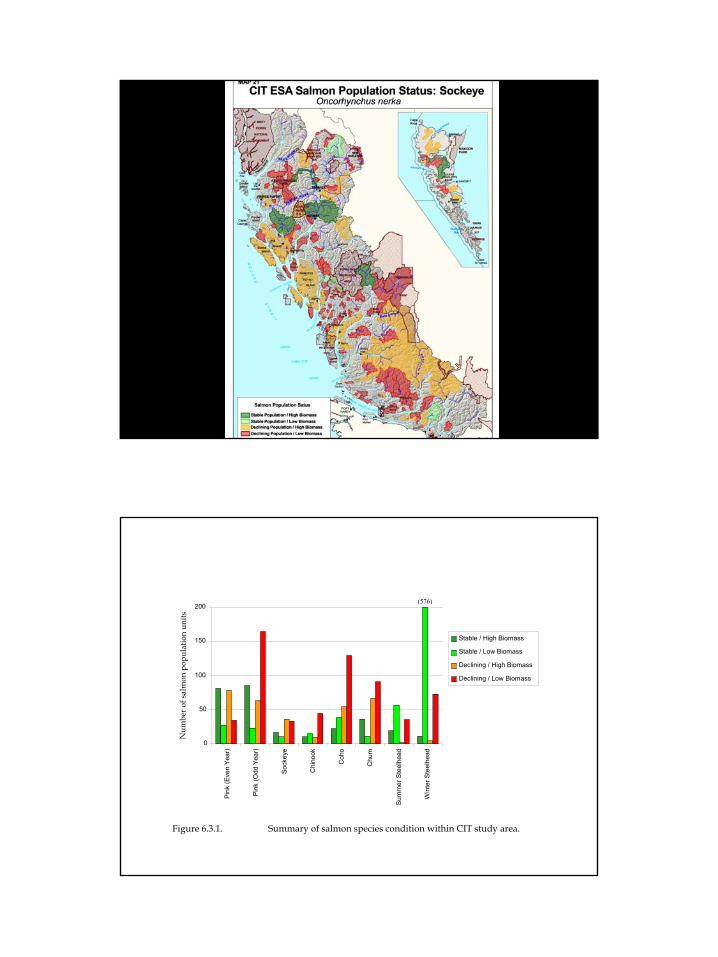
Stable / High Biomass
Stable / Low Biomass
Declining / High Biomass
Declining / Low Biomass
(576)
Figure 6.3.1. Summary of salmon species condition within CIT study area.
Num
ber o
f sal
mon
po p
u lat
i on
uni ts

19
0
2
4
6
8
10
12
14
16
18
Nass Skeena North Coast CentralCoast
Haida Gwaii
Stable / High BiomassStable / Low BiomassDeclining / High BiomassDeclining / Low Biomass
Figure 6.3.4. Summary of Sockeye condition by EDU.
Num
ber o
f sal
mon
po p
u lat
i on
uni ts
Representation AnalysesRepresentation Analyses
• The “coarse filter”• Represent range of natural variation along
environmental gradients• Protect high-quality examples of all
ecosystems in a region. • Ecosystems - Dynamic spatial assemblages of
communities that:– occur together in similar geomorphological patterns– are tied together by similar ecological processes or
environmental gradients – form a robust, cohesive and distinguishable spatial unit

20
TERRESTRIAL ECOSYSTEMS
• Terrestrial Ecosystem Analysis Units– Site productivity and BEC– BEC Variant x Site Index x Seral Stage – Distinguish between impacted and non-impacted • Productivity
– 3 classes: Low = 1-14, Medium = 15 – 21, and High = >22
• Seral Stage– Forest cover, ssPEM, image analysis– 3 classes: old growth forest, young intact forest,
logged forest
21
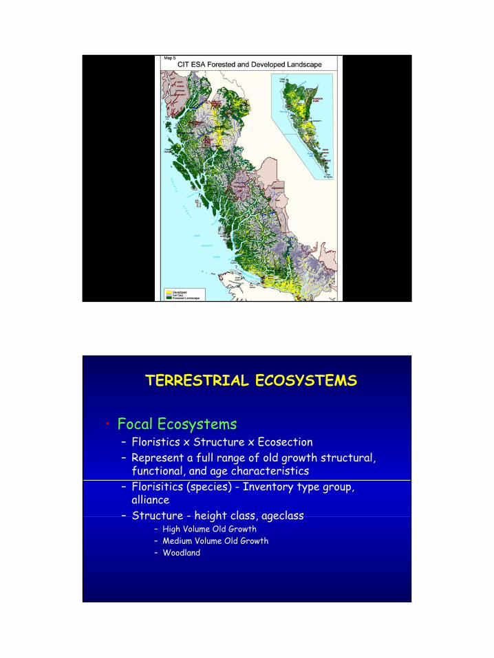
TERRESTRIAL ECOSYSTEMS
• Focal Ecosystems– Floristics x Structure x Ecosection– Represent a full range of old growth structural,
functional, and age characteristics– Florisitics (species) - Inventory type group,
alliance – Structure - height class, ageclass
– High Volume Old Growth– Medium Volume Old Growth– Woodland
22
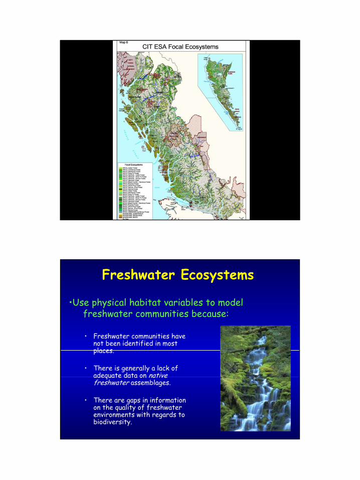
Freshwater Ecosystems
• Freshwater communities have not been identified in most places.
• There is generally a lack of adequate data on native freshwater assemblages.
• There are gaps in information on the quality of freshwater environments with regards to biodiversity.
•Use physical habitat variables to model freshwater communities because:
23
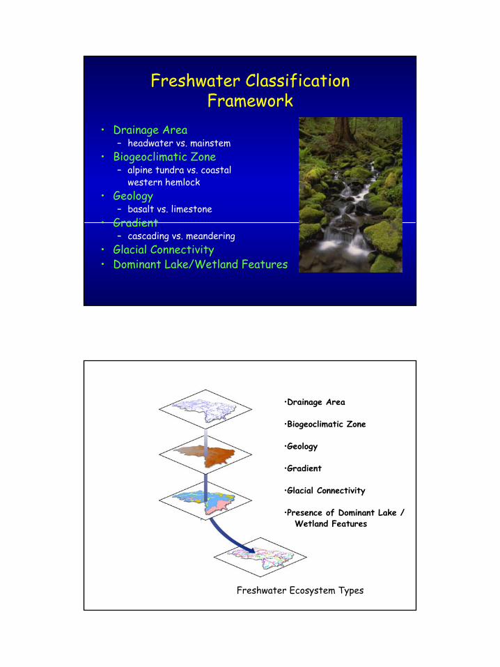
Freshwater Classification Framework
• Drainage Area– headwater vs. mainstem
• Biogeoclimatic Zone– alpine tundra vs. coastal
western hemlock• Geology
– basalt vs. limestone• Gradient
– cascading vs. meandering• Glacial Connectivity• Dominant Lake/Wetland Features
Freshwater Ecosystem Types
•Drainage Area
•Biogeoclimatic Zone
•Geology
•Gradient
•Glacial Connectivity
•Presence of Dominant Lake / Wetland Features

24
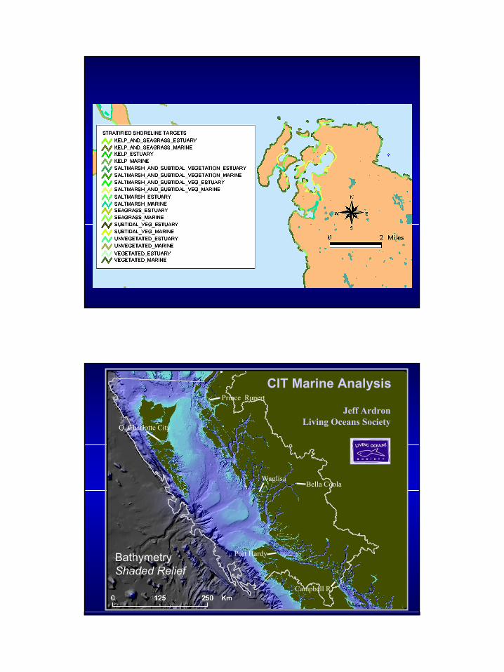
Marine Nearshore Ecosystem Representation
25
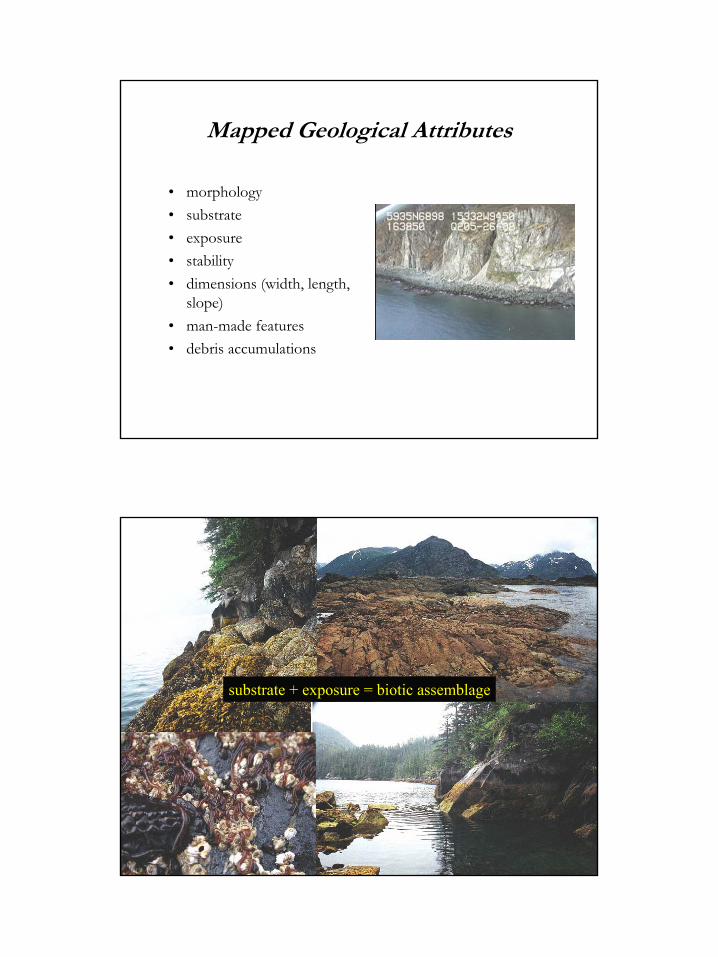
Mapped Geological Attributes
• morphology• substrate• exposure• stability• dimensions (width, length,
slope)• man-made features• debris accumulations
substrate + exposure = biotic assemblage
26
CIT Marine Analysis
Jeff ArdronLiving Oceans Society
Prince Rupert
Port Hardy
Bella CoolaWaglisa
Q. Charlotte City
Campbell R.
BathymetryShaded Relief
27
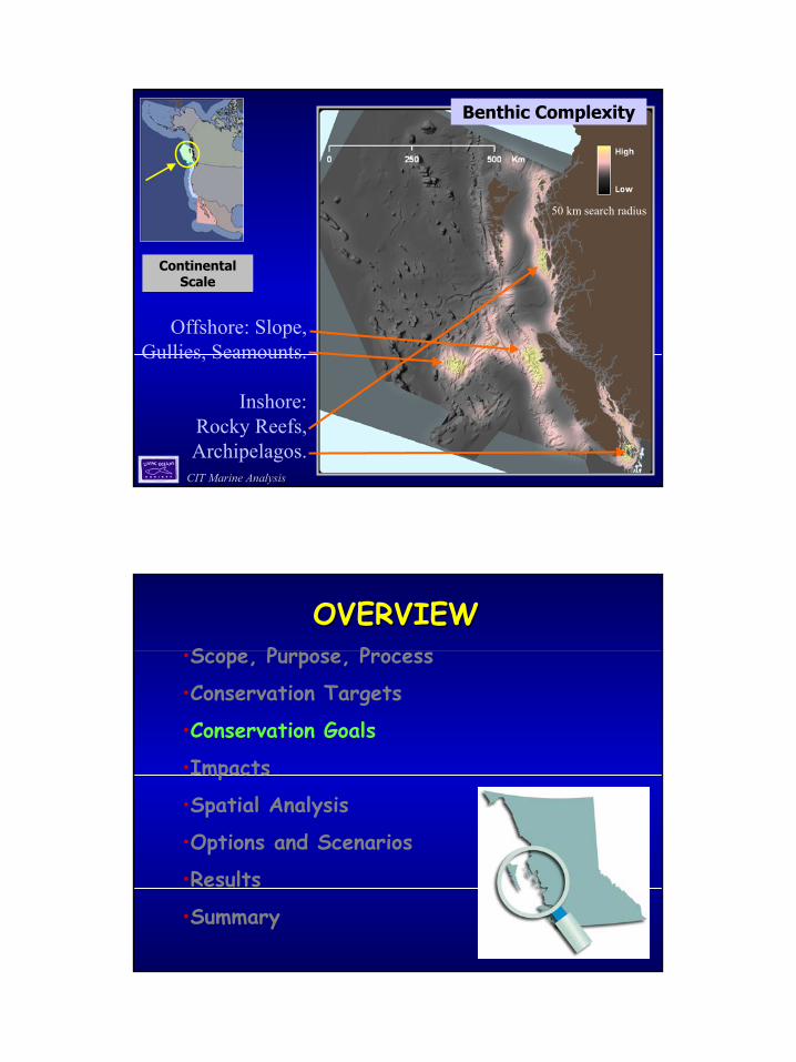
Benthic Complexity
Offshore: Slope, Gullies, Seamounts.
Inshore: Rocky Reefs, Archipelagos.
50 km search radius
Continental Scale
CIT Marine AnalysisCIT Marine Analysis
OVERVIEWOVERVIEW•Scope, Purpose, Process
•Conservation Targets
•Conservation Goals
•Impacts
•Spatial Analysis
•Options and Scenarios
•Results
•Summary
28
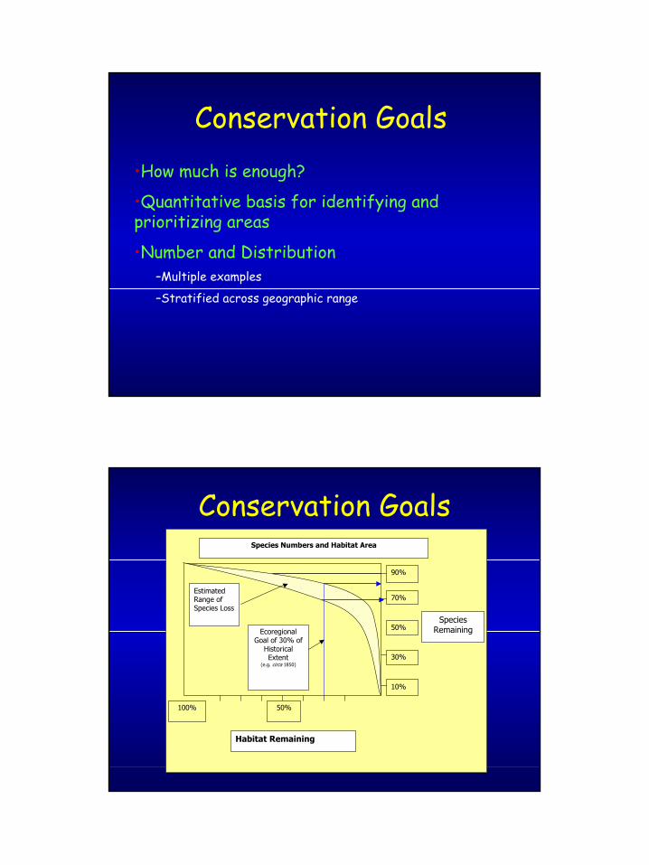
Conservation Goals•How much is enough?
•Quantitative basis for identifying and prioritizing areas
•Number and Distribution–Multiple examples
–Stratified across geographic range
Conservation Goals
Species Remaining
Habitat Remaining
100%
90%
70%
50%
30%
10%
50%
Species Numbers and Habitat Area
EcoregionalGoal of 30% of
Historical Extent
(e.g. circa 1850)
Estimated Range of Species Loss

29
Conservation Goals•Lack of Population Viability Assessments
•Available literature
•Consensus around 40 to 60% of a region
•40% lower responsible limit
•EBM 30 to 70% of natural variation
•ESA guideline: 30, 40, 50, 60 and 70% representation of targets
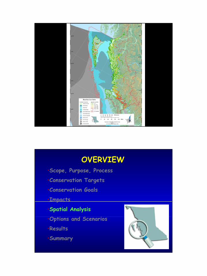
OVERVIEWOVERVIEW•Scope, Purpose, Process
•Conservation Targets
•Conservation Goals
•Impacts
•Spatial Analysis
•Options and Scenarios
•Results
•Summary

30
Wide-Ranging Carnivores
Condition Assessment
• Measuring overall impact – Urban/Agricultural Areas– Logged Area– Road Impact Area: 200m buffer around roads
(overlap between physical impacts (20m –200m) and indirect impacts (200m – 2 km)
– Overlapping impacts counted only once (greatly reduces effect of missing and patchy data)

31
Viability Assessment
Class Description
Intact1 no industrial impact; pristine
Intact2 < 2% area impacted; modified
Intact3 < 10% of area impacted and < 10% of area in proximity to rivers/streams impacted
Restoration1 < 15% of area impacted and < 0.6 km/km2 road density
Restoration2 < 25% of area impacted and < 0.6 km/km2
Developed > 25% of area impacted or > 0.6km/km2
road density
32
OVERVIEWOVERVIEW•Scope, Purpose, Process
•Conservation Targets
•Conservation Goals
•Impacts
•Spatial Analysis
•Options and Scenarios
•Results
•Summary
33
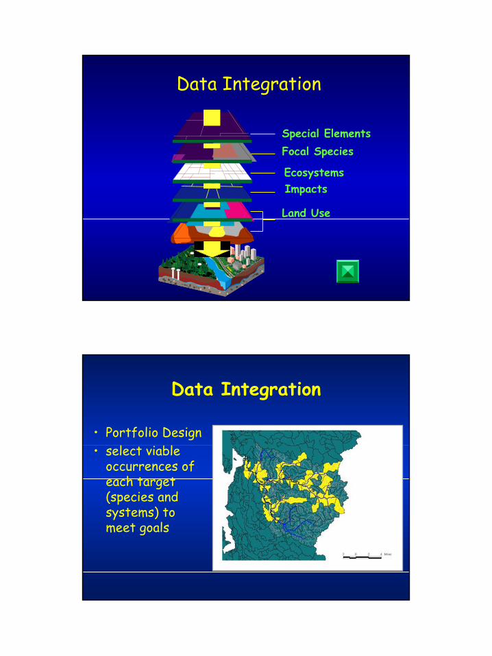
Special ElementsFocal Species
EcosystemsImpacts
Land Use
Data Integration
Data Integration
• Portfolio Design• select viable
occurrences of each target (species and systems) to meet goals
34
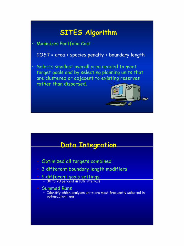
SITES Algorithm
COST = area + species penalty + boundary length
• Selects smallest overall area needed to meet target goals and by selecting planning units that are clustered or adjacent to existing reserves rather than dispersed.
• Minimizes Portfolio Cost
Data Integration
• Optimized all targets combined• 3 different boundary length modifiers • 5 different goals settings
– 30 to 70 percent in 10% intervals
• Summed Runs– Identify which analyses units are most frequently selected in
optimization runs

35
OVERVIEWOVERVIEW•Scope, Purpose, Process
•Conservation Targets
•Conservation Goals
•Impacts
•Spatial Analysis
•Options and Scenarios
•Results
•Summary
Options• Summary of all 300 SITES runs
– summed solution score out of 300
• Indicates the importance of each planning unit or watershed to the overall conservation solution
• Indication of “Value”, “irreplaceability”, “Utility”Summed Solution Score Quintile Conservation
Value Rating
> 180 Top 2/5 High
< 179, > 120 3/5 Medium
< 119, > 60 4/5 Low
< 60 5/5 Not Ranked
36
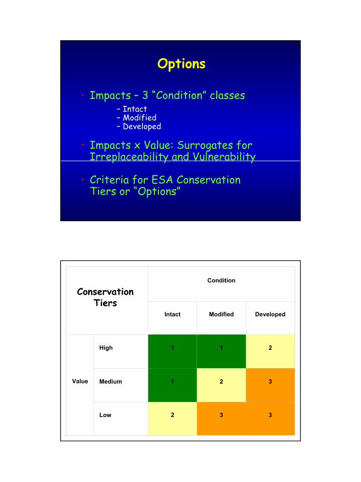
Options
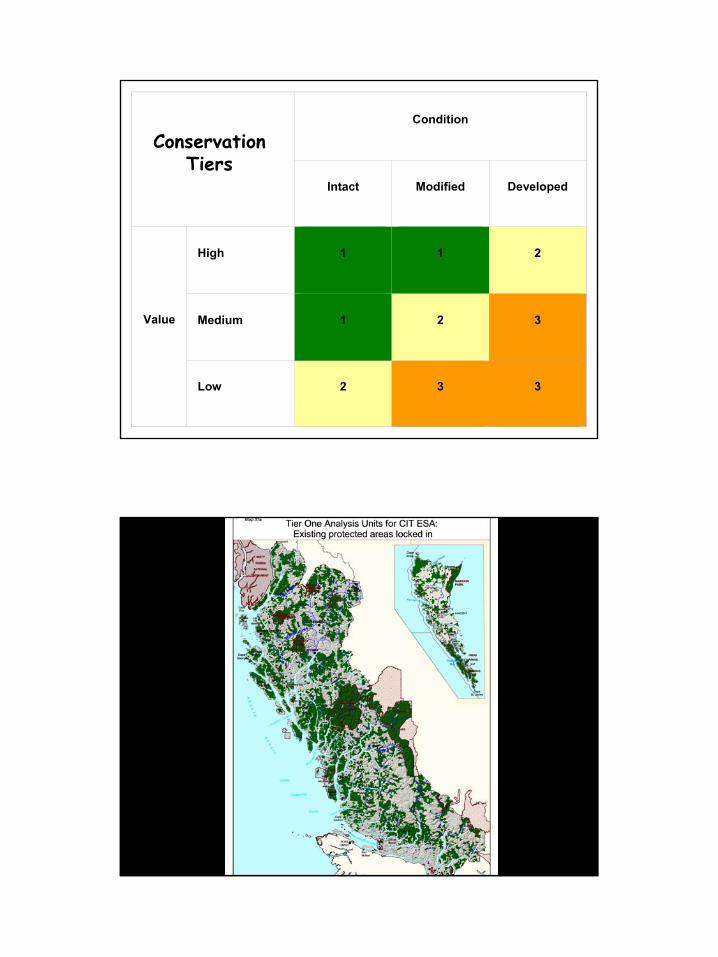
• Impacts – 3 “Condition” classes– Intact– Modified– Developed
• Impacts x Value: Surrogates for Irreplaceability and Vulnerability
• Criteria for ESA Conservation Tiers or “Options”
Condition
Intact Modified Developed
Value
High 1 1 2
Medium 1 2 3
Low 2 3 3
ConservationTiers
37
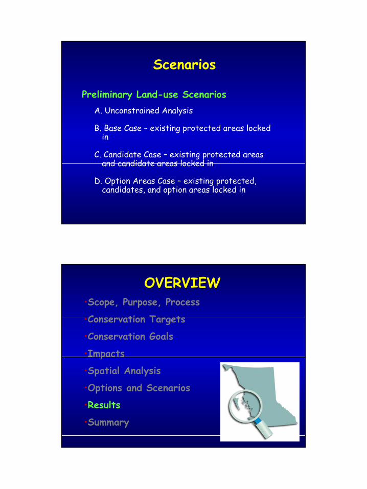
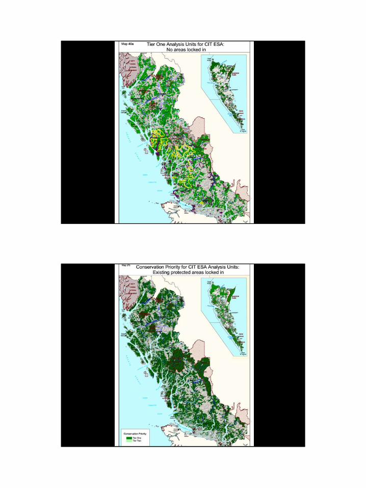
Scenarios
Preliminary Land-use ScenariosA. Unconstrained Analysis
B. Base Case – existing protected areas locked in
C. Candidate Case – existing protected areas and candidate areas locked in
D. Option Areas Case – existing protected, candidates, and option areas locked in
OVERVIEWOVERVIEW•Scope, Purpose, Process
•Conservation Targets
•Conservation Goals
•Impacts
•Spatial Analysis
•Options and Scenarios
•Results
•Summary

38

39
Fig 6.3 Goal performance for CIT ESA Conservation targets under exisiting and proposed protected area scenarios
(Candidate and Options areas limited to Central Coast LRMP Boundaries)
0
0.05
0.1
0.15
0.2
0.25
0.3
0.35
0.4
0.45
12% 30% 50% 70% 100%
Goal threshold option
Prop
ortio
n of
targ
ets
mee
ting
goal
th
resh
old
Existing ProtectedAreas
Existing plusCandidates
Existing plusCandidates andOption Areas
Protected Area Scenario
Fig 6.2 Progress Toward Goals for CIT ESA SITES Summed Solutions: Existing Protected Areas Locked In.
0
0.2
0.4
0.6
0.8
1
1.2
10 20 30 40 50 60 70 80 90
Percent of study area in conservation solution
Prop
ortio
n of
targ
ets
for w
hich
goa
l th
resh
old
is re
ache
d or
exc
eede
d
100705030
Goal Threshold
40
Condition
Intact Modified Developed
Value
High 1 1 2
Medium 1 2 3
Low 2 3 3
ConservationTiers
•Average Approx.3000 Ha
•~ 7000 watersheds
41
•Average Approx.3000 Ha
•~ 7000 watersheds
•Average Approx.3000 Ha
•~ 7000 watersheds
42
•Average Approx.3000 Ha
•~ 7000 watersheds
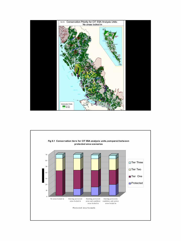
0
10
2 0
3 0
4 0
50
6 0
70
No areas lo cked in Exis t ing p ro tectedareas lo cked in
Exis it ing p ro tectedareas and cand id ate
areas lo cked in
Exis ting p ro tected ,cand id ate, and o p t io n
areas lo cked in
P ro t e c t e d A re a S c e na rio
Fig 6.1 Conservation tiers for CIT ESA analysis units,compared between protected area scenarios
Tier Three
Tier Two
Tier One
Protected

43
•Average Approx.3000 Ha
•~ 7000 watersheds

44

45
46
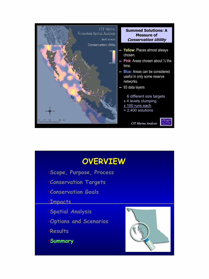
Yellow: Places almost always chosen.Pink: Areas chosen about ½ the time.Blue: Areas can be considered useful in only some reserve networks.93 data layers
6 different size targetsx 4 levels clumpingx 100 runs each= 2,400 solutions
Summed Solutions: A Measure of
Conservation Utility
CIT Marine AnalysisCIT Marine Analysis
OVERVIEWOVERVIEW•Scope, Purpose, Process
•Conservation Targets
•Conservation Goals
•Impacts
•Spatial Analysis
•Options and Scenarios
•Results
•Summary

47
Next Steps
• Integrate marine, and terrestrial/ freshwater results
• Alternative LRMP scenarios • Alternative reporting units• Post hoc analysis• Conclusions• Final database