Embed Size (px)
Citation preview

ECSS-E-HB-60-10A14 December 2010
Space engineeringControl performance guidelines
ECSS SecretariatESA-ESTEC
Requirements & Standards Division
Noordwijk, The Netherlands
ECSS-E-HB-60-10A14 December 2010
ForewordThis Handbook is one document of the series of ECSS Documents intended to be used as supporting material for ECSS Standards in space projects and applications. ECSS is a cooperative effort of the European Space Agency, national space agencies and European industry associations for the purpose of developing and maintaining common standards.Best practises in this Handbook are defined in terms of what can be accomplished, rather than in terms of how to organize and perform the necessary work. This allows existing organizational structures and methods to be applied where they are effective, and for the structures and methods to evolve as necessary without rewriting the standards and Handbooks.This handbook has been prepared by the ECSS-E-HB-60-10 Working Group, reviewed by the ECSS Executive Secretariat and approved by the ECSS Technical Authority.
DisclaimerECSS does not provide any warranty whatsoever, whether expressed, implied, or statutory, including, but not limited to, any warranty of merchantability or fitness for a particular purpose or any warranty that the contents of the item are error-free. In no respect shall ECSS incur any liability for any damages, including, but not limited to, direct, indirect, special, or consequential damages arising out of, resulting from, or in any way connected to the use of this document, whether or not based upon warranty, business agreement, tort, or otherwise; whether or not injury was sustained by persons or property or otherwise; and whether or not loss was sustained from, or arose out of, the results of, the item, or any services that may be provided by ECSS
Published by: ESA Requirements and Standards DivisionESTEC, P.O. Box 299,2200 AG NoordwijkThe Netherlands
Copyright: 2010© by the European Space Agency for the members of ECSS
2

ECSS-E-HB-60-10A14 December 2010
Change log
ECSS-E-HB-60-10A14 December 2010
First issue
3

ECSS-E-HB-60-10A14 December 2010
Table of contents
Change log.........................................................................................................3
Introduction........................................................................................................9
1 Scope.............................................................................................................11
2 References....................................................................................................12
3 Terms, definitions and abbreviated terms.................................................133.1 Terms from other documents...........................................................................13
3.2 Terms specific to the present handbook..........................................................13
3.3 Abbreviated terms............................................................................................17
4 General outline for control performance process.....................................194.1 The general control structure...........................................................................19
4.1.1 Description of the general control structure – Extension to system level....................................................................................................19
4.1.2 General performance definitions........................................................20
4.1.3 Example – Earth observation satellite...............................................21
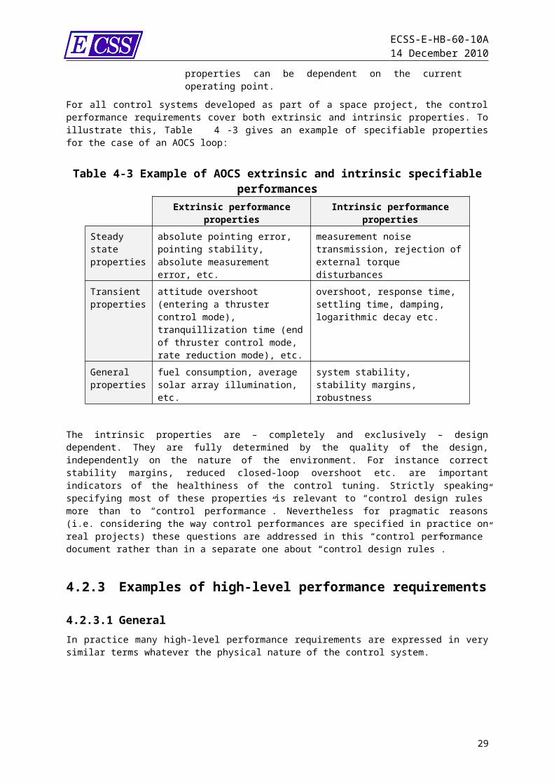
4.2 Review of generic performance specification elements...................................22
4.2.1 General..............................................................................................22
4.2.2 Preliminary remark on intrinsic and extrinsic performance properties22
4.2.3 Examples of high-level performance requirements...........................24
4.2.4 Formalising requirements through performance indicators...............26
4.3 Overview on performance specification and verification process....................28
4.3.1 Introduction........................................................................................28
4.3.2 Requirements capture & dissemination.............................................29
4.3.3 Performance verification....................................................................30
4.3.4 Control performance engineering tasks during development phases32
5 Extrinsic performance – error indices and analysis methods..................395.1 Introduction......................................................................................................39
5.2 Performance and measurement error indices.................................................39
4
ECSS-E-HB-60-10A14 December 2010
5.2.1 Definition of error function..................................................................39
5.2.2 Definition of error indices...................................................................40
5.2.3 Common performance error indices..................................................40
5.2.4 Common knowledge error indices.....................................................42
5.3 Formulation of performance requirements using error indices........................43
5.3.1 Structure of a requirement.................................................................43
5.3.2 Choice of error function......................................................................43
5.3.3 Use of error indices............................................................................44
5.3.4 Statistical interpretation of a requirement..........................................44
5.3.5 Formulation of Knowledge Requirements..........................................47
5.4 Assessing compliance with a performance requirement.................................47
5.4.1 Overview............................................................................................47
5.4.2 Experimental approach......................................................................48
5.4.3 Numerical simulations........................................................................48
5.4.4 Use of an error budget.......................................................................50
5.5 Performance error budgeting...........................................................................51
5.5.1 Overview............................................................................................51
5.5.2 Identifying errors................................................................................51
5.5.3 Statistics of contributing terms...........................................................52
5.5.4 Combination of error terms................................................................53
5.5.5 Comparison with requirements..........................................................54
5.5.6 Practical use of a budget (Synthesis)................................................54
6 Intrinsic performance indicators for closed-loop controlled systems....576.1 Overview..........................................................................................................57
6.2 Closed-loop controlled systems.......................................................................57
6.2.1 General closed-loop structure............................................................57
6.2.2 General definitions for closed-loop controlled systems.....................58
6.3 Stability of a closed-loop controlled system.....................................................60
6.4 Stability margins..............................................................................................60
6.4.2 Stability margins for SISO LTI systems.............................................61
6.4.3 Stability margins for MIMO LTI system – S and T criteria.................63
6.4.4 Why specifying stability margins?......................................................65
6.5 Level of robustness of a closed-loop controlled system..................................66
6.6 Time & Frequency domain behaviour of a closed-loop controlled system......66
6.6.1 Overview............................................................................................66
6.6.2 Time domain indicators (transient)....................................................66
6.6.3 Frequency domain performance indicators.......................................68
5
ECSS-E-HB-60-10A14 December 2010
6.7 Formulation of performance requirements for closed-loop controlled systems71
6.7.1 General..............................................................................................71
6.7.2 Structure of a requirement.................................................................71
6.7.3 Specification for general systems (possibly MIMO, coupled or nested loops).................................................................................................72
6.7.4 Example of stability margins requirement..........................................72
6.8 Assessing compliance with performance requirements...................................73
6.8.1 Guidelines for stability and stability margins verification....................73
6.8.2 Methods for (systematic) robustness assessment.............................74
7 Hierarchy of control performance requirements.......................................757.1 Overview..........................................................................................................75
7.2 From top level requirements down to design rules..........................................75
7.2.1 General..............................................................................................75
7.2.2 Top level requirements......................................................................75
7.2.3 Intermediate level requirements........................................................76
7.2.4 Lower level requirements – Design rules...........................................76
7.3 The risks of counterproductive requirements...................................................77
7.3.1 An example of counterproductive requirement..................................77
7.3.2 How to avoid counterproductive control performance requirements?77
Annex A LTI systems......................................................................................78A.1 Overview..........................................................................................................78
A.2 General properties of LTI systems...................................................................78
A.2.1 Simplified structure of a closed-loop controlled system.....................78
A.2.2 Representation of LTI systems..........................................................79
A.3 On stability margins of SISO and MIMO LTI systems.....................................81
A.3.1 Interpretation of stability margins.......................................................81
A.3.2 Analysis of stability margins – some illustrations...............................83
Annex B Appendices to clause 5: Guidelines and mathematical elements85B.1 Error Indices with domains other than time.....................................................85
B.2 Considerations regarding time intervals..........................................................86
B.3 Relationship between error indices and physical quantities............................86
B.4 Statistics for Monte Carlo Minimum Number of Runs......................................88
B.5 Determining the error PDFs.............................................................................89
B.5.1 Overview............................................................................................89
B.5.2 White noise........................................................................................89
B.5.3 Biases................................................................................................90
6
ECSS-E-HB-60-10A14 December 2010
B.5.4 Uniform random errors.......................................................................91
B.5.5 Harmonic errors.................................................................................91
B.5.6 Drift Errors..........................................................................................92
B.5.7 Transient Errors.................................................................................93
B.5.8 Others (General Analysis Methods)...................................................94
B.5.9 Distributions of Ensemble Parameters..............................................95
B.6 Mathematics of an Error Budget......................................................................96
B.6.1 Probability distributions and the statistical interpretation...................96
B.6.2 Exact error combination methods......................................................97
B.6.3 Alternative approximation formulae...................................................98
Annex C Satellite AOCS case study..............................................................99C.1 Introduction......................................................................................................99
C.2 Satellite AOCS architecture.............................................................................99
C.3 From Image quality to AOCS requirements.....................................................99
C.4 Formulation of the requirements C.3a1 to C.3a4 using error indices............102
C.4.1 General............................................................................................102
C.4.2 Choice of signal error function.........................................................103
C.4.3 Choice of error indices and maximum values..................................103
C.4.4 Assigning a probability density function (PDF)................................103
C.4.5 Choice of statistical interpretation (temporal, ensemble, mixed…)..104
C.4.6 Requirements formulation................................................................104
C.5 Formulation of requirements C.3b1 and C.3b2..............................................105
C.6 Control Performance verification principles...................................................105
C.6.1 Choice of verification method..........................................................105
C.6.2 Compiling the error budget (requirements C.3a1 to C.3a4).............106
C.6.3 Assessing compliance to control loop requirements C.3b1 and C.3b2111
C.7 Performance budget examples......................................................................112
C.7.1 Overview..........................................................................................112
C.7.2 Pointing Knowledge Budget.............................................................112
C.7.3 Pointing budget................................................................................115
C.7.4 Pointing stability Budget (Requirements C.3a3 and C.3a4)............117
Figures
Figure 4-1 General control structure, ECSS-E-HB-60A...............................................19
Figure 4-2 General control structure extended up to system level...............................20
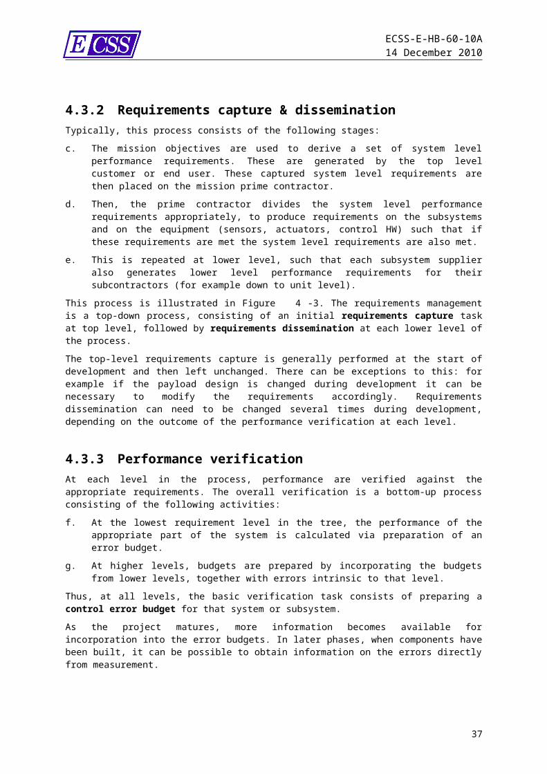
Figure 4-3 Example of requirements capture and dissemination for a typical AOCS case.............................................................................................................31
7
ECSS-E-HB-60-10A14 December 2010
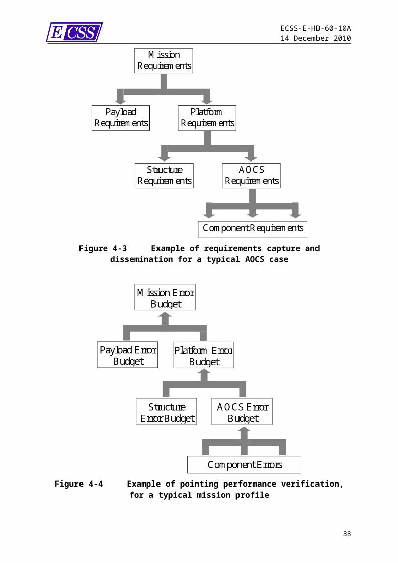
Figure 4-4 Example of pointing performance verification, for a typical mission profile.31
Figure 5-1 Illustration of the different ways of meeting a requirement.........................45
Figure 5-2 Statistics for the different statistical interpretations. L-R: temporal interpretation, ensemble interpretation, mixed interpretation......................45
Figure 6-1 Simplified scheme for a closed-loop controlled system..............................58
Figure 6-2 Example of gain and phase margins identification......................................63
Figure 6-3 Illustration of the transient response indicators...........................................67
Figure 6-4 Bandwidth, cut-off frequency and rejection of resonances.........................70
Tables
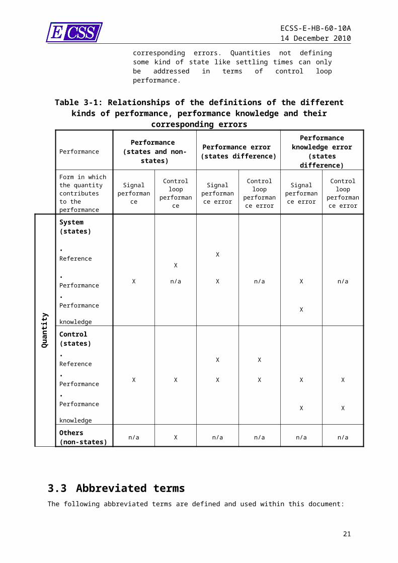
Table 3-1: Relationships of the definitions of the different kinds of performance, performance knowledge and their corresponding errors............................17
Table 4-1 Example of a control structure breakdown for an Earth observation satellite22
Table 4-2 Example of AOCS extrinsic and intrinsic specifiable performances...........23
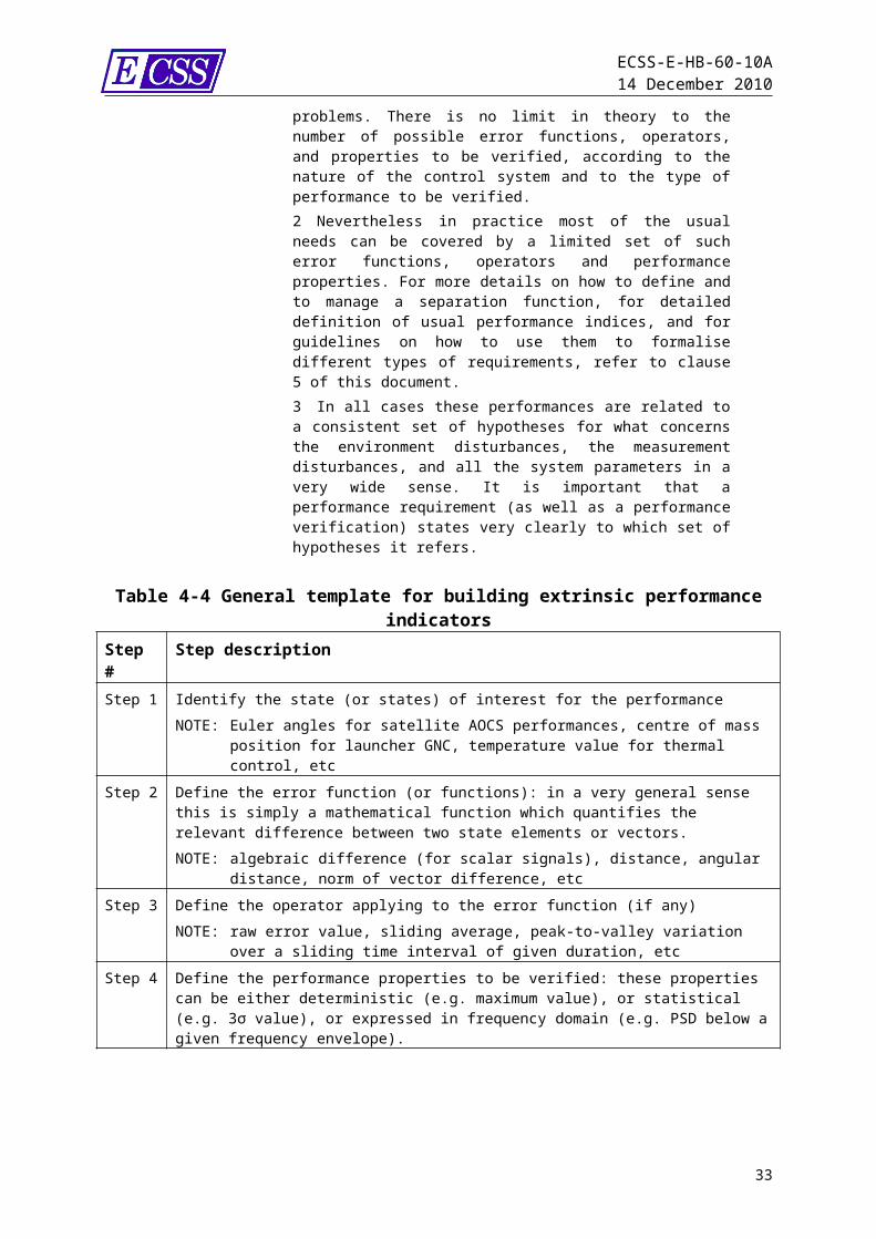
Table 4-3 General template for building extrinsic performance indicators..................27
Table 4-4 Summary of control performance engineering tasks...................................29
Table 4-5 Summary of the control performance management activities during the phases of mission development (guidelines only).......................................32
Table 4-6 Control performance engineering inputs, tasks and outputs, Phase 0/A....33
Table 4-7 Control performance engineering inputs, tasks and outputs, Phase B.......35
Table 4-8 Control performance engineering inputs, tasks and outputs, Phase C/D.. .37
Table 4-9 Control performance engineering inputs, tasks and outputs, Phase E/F....38
Table 5-1 Minimum number of simulation runs required to verify a requirement at confidence level Pc to a verification confidence of 95 %...........................50
Table 5-2 Example of a table used for a performance budget (APE for Euler angles)56
Table 6-1 Formulas for the usual SISO stability margins............................................62
8
ECSS-E-HB-60-10A14 December 2010
Introduction
This document focuses on the specific issues raised by managing all performance aspects of control systems in the frame of space projects. It provides a set of practical definitions, engineering rules, recommendations and guidelines to be used when specifying or verifying the performance of a general control system; attention was paid by the authors to keep the application field as open as possible, and not to restrict to a specific domain – such as spacecraft attitude control for example. It is not intended to substitute to textbook material on automatic control theory. The readers and the users are assumed to possess general knowledge of control system engineering and its applications to space missions. Nevertheless when required – to avoid any risks of ambiguity for example, or for the clearness of the presentation – some basic definitions and rules are provided in dedicated annexes.This document was originally intended to focus on the specific case of pointing systems and AOCS, starting from an existing ESA handbook [Pointing Error Handbook, ESA-NCR-502], to be updated, completed, and extended to be built up as an applicable ECSS document. But after reviewing the scope, this approach appeared somewhat restrictive:
restricting performance concepts to “pointing” does not allow to deal with problems such as thermal control, position control (robotics), or more generally any other type of control systems, even though these problems share the same theoretical framework; AOCS is one major contributor to the overall system pointing performance, yet not the only one: misalignments, thermoelastic effects, payload behaviour, etc. all contribute to the final performance. This remark can be extended to general systems, considering that the controlled part is but one of the contributors.
Accounting for these remarks led to extending the initial scope of this document. The upgraded objective is to set up a generalised framework introducing performance definitions, performance indices and budget calculations. “Generalised” is understood here in two directions:
transversally, so as to be applicable independently on the physical nature of the control system (not only pointing), and vertically, in the sense that in many practical situations the proposed definitions and techniques can also apply to any part of the system (basically to the controlled part, but not restrictively). This should assure consistency between the performances indices (error budgets) of the complete system and of the controlled system part. Motivation is also that dedicated but generic methods for budget breakdown can be applied on different levels i.e. on system level and on controlled system level.
NOTE 1 The idea of defining a general framework applying from equipment level to system level is driven by a concern for technical and conceptual consistency. In a later phase, relevant system aspects can be transferred or copied to the appropriate System Engineering standard – if found more convenient.
9
ECSS-E-HB-60-10A14 December 2010
NOTE 2 The general control structure from the Control Engineering handbook [ECSS-E-HB-60A, Figure 4-1] has been extended in support, showing also the system performance in the output (Figure 4-2 of this handbook)NOTE 3 The objective of this document is not to cover the high level system or mission performance aspects, which clearly belong to a different category.
In addition to this will for general and generic concepts, a clause of this document covers the performance issues which are more specific for the controlled systems themselves (mainly involving feedback loops in practice) or which are based on well-known control methods. The need for this clause arises as such systems call for particular technical know-how and feature specific performance indicators that require additional insight. For example: stability and robustness properties, transient responses (settling time, response time etc.) and frequency domain indicators.Although this document is designed to be as general as possible, clearly in practice pointing and AOCS issues are the most demanding space engineering disciplines in terms of control systems. They are covered by an informative annex of the document which declines the general concepts and illustrates how pointing issues can be managed as a special case of vector-type data on a high resolution Earth observation mission.Driven by a similar concern for illustration on space engineering applications of practical interest, another annex of the document shows how to decline the general concepts to deal with the control performance issue arisen by robotics applications.
10

ECSS-E-HB-60-10A14 December 2010
1Scope
This Handbook deals with control systems developed as part of a space project. It is applicable to all the elements of a space system, including the space segment, the ground segment and the launch service segment.It addresses the issue of control performance, in terms of definition, specification, verification and validation methods and processes. The handbook establishes a general framework for handling performance indicators, which applies to all disciplines involving control engineering, and which can be declined as well at different levels ranging from equipment to system level. It also focuses on the specific performance indicators applicable to the case of closed-loop control systems.Rules and guidelines are provided allowing to combine different error sources in order to build up a performance budget and to assess the compliance with a requirement.This version of the handbook does not cover control performance issues in the frame of launch systems.
11
ECSS-E-HB-60-10A14 December 2010
2References
ECSS-S-ST-00-01 ECSS System - Glossary of termsECSS-E-ST-10 Space engineering – System engineering
general requirementsECSS-E-ST-60-10 Space engineering – Control performanceECSS-E-ST-60-20 Space engineering – Stars sensors
terminology and performance specificationsECSS-E-HB-60 Space engineering – Control engineering
handbookECSS-M-ST-40 Space project management – Configuration
and information management
12
ECSS-E-HB-60-10A14 December 2010
3Terms, definitions and abbreviated terms
3.1 Terms from other documentsFor the purpose of this document, the terms and definitions from ECSS-S-ST-00-01 apply.
3.2 Terms specific to the present handbook3.2.1 control performance (state)quantified output of a controlled system
NOTE 1 Depending on the context, the control performance is realised either as signal performance or as control loop performance.NOTE 2 Can also be applied to a control system.
3.2.2 control (performance) knowledge (state)estimated control performance after measurement and processing, if any
NOTE The control performance knowledge is not necessarily the best available knowledge of the control performance. The achieved accuracy and the allowed deviation (control performance knowledge error) depends on the application.
3.2.3 control reference (state)ideal reference input, desired state or reference state of controlled part of the plant
3.2.4 domain variableindependent variable which can be used to put some dependent quantity into a certain order
NOTE This comprises continuous time, discrete time, N-dimensional space, etc.
3.2.5 ergodicityproperty of a stochastic process such that its ensemble and time statistical properties are identical. Ergodicity allows to transfer the statistical results of a single realisation of a stochastic process to the whole ensemble
13
ECSS-E-HB-60-10A14 December 2010
NOTE (Weak) stationarity is prerequisite for (weak) ergodicity.
3.2.6 error index parameter isolating a particular aspect of the time variation of a performance error or knowledge error
3.2.7 extrinsic performanceelement of performance related to the response of the system to its interaction with the outer world (control reference signal, error sources and other disturbances)
NOTE 1 for example the pointing error of a satellite is relevant to this category of extrinsic performance (it depends on the disturbing torques and on the measurement noises)NOTE 2 can also be defined in opposition to intrinsic performance
3.2.8 intrinsic performanceelement of performance related to the intrinsic properties of the system, independently on its interaction with the outer world (control reference, the nature and the amplitude of the error sources and other disturbances)
NOTE 1 for example the stability of a closed-loop controlled system is relevant to this category of intrinsic performancesNOTE 2 can also be defined in opposition to extrinsic performanceNOTE 3 “I have some of my properties purely in virtue of the way I am. (My mass is an example.) I have other properties in virtue of the way I interact with the world. (My weight is an example.) The former are the intrinsic properties, the latter are the extrinsic properties” [Weatherson, Brian, "Intrinsic vs. Extrinsic Properties", The Stanford Encyclopedia of Philosophy (Fall 2004 Edition), Edward N. Zalta (ed.)]
3.2.9 individual error source elementary physical characteristic or process originating from a well-defined source which contributes to a performance error or a performance knowledge error
NOTE For example sensor noise, sensor bias, actuator noise, actuator bias, disturbance forces/torques (e.g. micro-vibrations, manoeuvres, external or internal subsystem motions), friction force/torque, misalignments, thermal distortions, assembly distortions, digital quantization, control law performance (steady state error), jitter, etc.
3.2.10 performance error (state difference)deviation of a performance from its reference; realised as control (signal or control loop) performance error or system performance error, depending on the context
3.2.11 performance error indicator (state difference)any quantity suitable to define the performance error or performance knowledge error of a controlled system or one of its parts. Examples are signal error functions, signal error indices or control loop performance indicators
14
ECSS-E-HB-60-10A14 December 2010
3.2.12 performance knowledge error (state difference)deviation of a performance from its performance knowledge; realised as control (signal or control loop) knowledge error or system performance knowledge error, depending on the context
3.2.13 robustnessability of a controlled system to maintain some performance or stability characteristics in the presence of plant, sensors, actuators and/or environmental uncertainties
NOTE 1 Performance robustness is the ability to maintain performance in the presence of defined bounded uncertainties.NOTE 2 Stability robustness is the ability to maintain stability in the presence of defined bounded uncertainties.
3.2.14 signal performance (state)characteristic output signal of the plant; either a control performance or a system performance
3.2.15 stabilityproperty that defines the specified static and dynamics limits of a system[ECSS-E-HB-60A]
3.2.16 signal stabilityvariations of a signal over a given time frame
NOTE The signal stability belongs to the category of extrinsic performances.
3.2.17 system stabilityability of a system submitted to small external disturbances to remain indefinitely in a bounded domain around an equilibrium position or around an equilibrium trajectory
NOTE 1 This property is essential for closed-loop control design. But it also applies to uncontrolled systems; for example a free body spinning about an intermediate axis of inertia is unstable.NOTE 2 As clearly stated signal stability and system stability are different properties which apply in different contexts. The risk for confusion is minor in practice. It is proposed to keep the wording “stability” unchanged in the frame of this standard, clarifying the current meaning should any ambiguity occur.
3.2.18 stability marginmaximum excursion of the parameters describing a given system for which the system remains stable
NOTE 1 Stability margins belong to the category of intrinsic performances (they do not depend on the system inputs and disturbances).NOTE 2 The most frequent stability margins defined in classical control design are the gain margin, the phase margin, the modulus margin, and – less frequently – the delay margins (see Clause 6 of this document).
15
ECSS-E-HB-60-10A14 December 2010
3.2.19 stationarityproperty of a stochastic process such that its statistical behaviour is time independent
NOTE Weak stationarity comprises only the time independence of the first two statistical moments (mean and variance).
3.2.20 statistical ensembleset of all physically possible combinations of values of parameters which describe a controlled system
3.2.21 steady statesituation where all internal and external parameters of a system (states, control reference, environment, disturbances) vary slowly compared to the intrinsic time constants of the system
NOTE 1 steady state can also be defined by opposition to transient eventsNOTE 2 “steady” does not mean that all parameters are invariant. For example a controlled system can be in steady state although its control reference is moving (tracking systems).
3.2.22 stochastic processfunction defining a random variable for each time instance (discrete or continuous) and each realisation of a statistical ensemble
3.2.23 system performance (state)quantified output of the sum of the controlled and uncontrolled parts of the plant. In most cases, the system performance is realised as a signal performance
3.2.24 system (performance) knowledge (state)estimated system performance after measurement and processing, if any. If no additional open-loop sensor is available, the system performance knowledge is identical to the control performance knowledge
NOTE The system performance knowledge is not necessarily the best available knowledge of the system performance. The achieved accuracy and the allowed deviation (system performance knowledge error) depends on the application.
3.2.25 system reference (state)desired state or reference state of the sum of the controlled and uncontrolled parts of the plant
3.2.26 transient eventsituation where one at least of the internal or external parameters of a system (control reference, environment, disturbances) exhibits a stiff variation compared to the intrinsic time constants of the system
NOTE Can also be defined by opposition to steady state.
3.2.27 tracking systemcontrol system requested to follow a given reference profile
16
ECSS-E-HB-60-10A14 December 2010
NOTE Table 3-1 summarizes the main relationships for the definitions of the different kinds of performance, performance knowledge and their corresponding errors. Quantities not defining some kind of state like settling times can only be addressed in terms of control loop performance.
Table 3-1: Relationships of the definitions of the different kinds of performance, performance knowledge and their corresponding
errors
PerformancePerformance
(states and non-states)
Performance error (states difference)
Performance knowledge error
(states difference)Form in which the quantity contributes to the performance
Signal performan
ce
Control loop
performance
Signal performance error
Control loop
performance error
Signal performance error
Control loop
performance error
Qua
ntit
y
System (states)
• ReferenceX
X
• Performance X n/a X n/a X n/a
• Performance knowledge
X
Control (states)• Reference X X• Performance X X X X X X
• Performance knowledge
X X
Others (non-states) n/a X n/a n/a n/a n/a
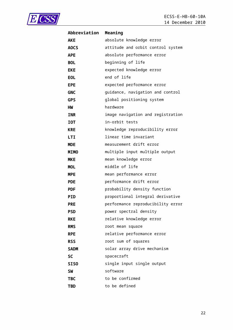
3.3 Abbreviated termsThe following abbreviated terms are defined and used within this document:
Abbreviation MeaningAKE absolute knowledge errorAOCS attitude and orbit control systemAPE absolute performance errorBOL beginning of lifeEKE expected knowledge error
17
ECSS-E-HB-60-10A14 December 2010
EOL end of lifeEPE expected performance errorGNC guidance, navigation and controlGPS global positioning systemHW hardwareINR image navigation and registrationIOT in-orbit testsKRE knowledge reproducibility errorLTI linear time invariantMDE measurement drift errorMIMO multiple input multiple outputMKE mean knowledge errorMOL middle of lifeMPE mean performance errorPDE performance drift errorPDF probability density functionPID proportional integral derivativePRE performance reproducibility errorPSD power spectral densityRKE relative knowledge errorRMS root mean squareRPE relative performance errorRSS root sum of squaresSADM solar array drive mechanismSC spacecraftSISO single input single outputSW softwareTBC to be confirmedTBD to be defined
18
ECSS-E-HB-60-10A14 December 2010
4General outline for control performance
process
4.1 The general control structure
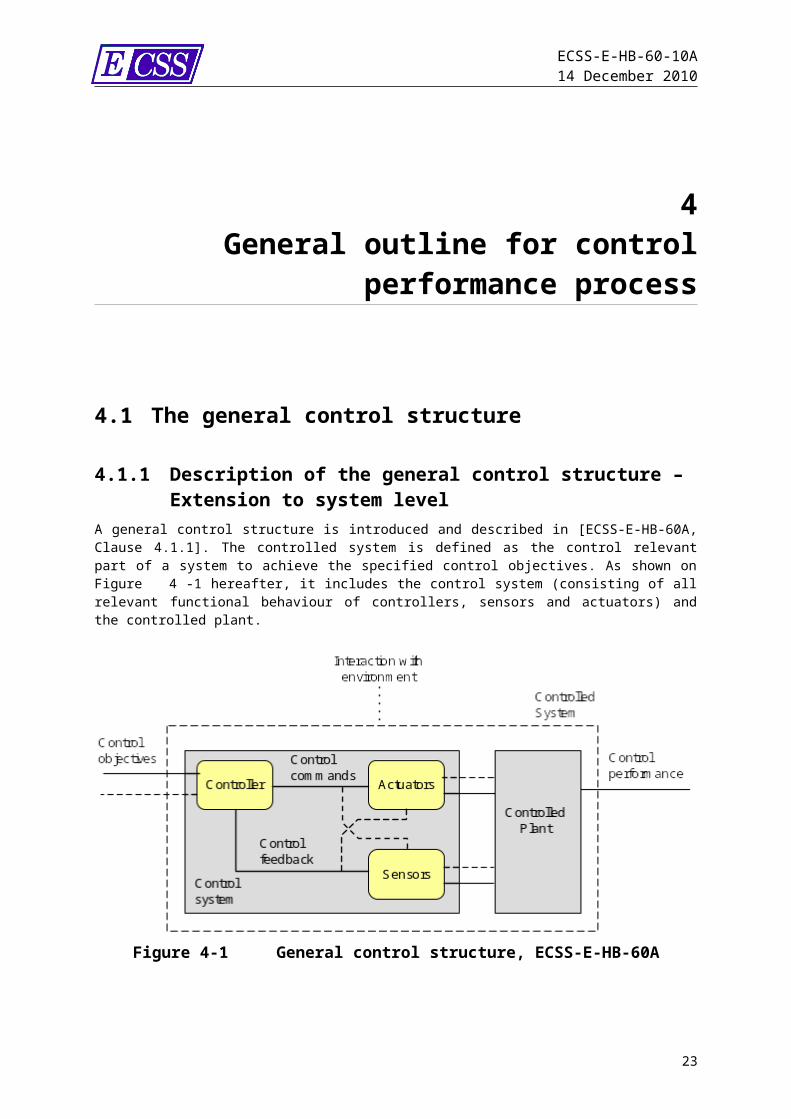
4.1.1 Description of the general control structure – Extension to system level
A general control structure is introduced and described in [ECSS-E-HB-60A, Clause 4.1.1]. The controlled system is defined as the control relevant part of a system to achieve the specified control objectives. As shown on Figure 4-1 hereafter, it includes the control system (consisting of all relevant functional behaviour of controllers, sensors and actuators) and the controlled plant.
Figure 4-1General control structure, ECSS-E-HB-60A
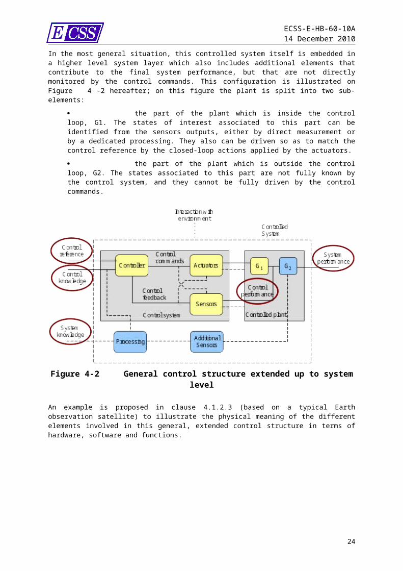
In the most general situation, this controlled system itself is embedded in a higher level system layer which also includes additional elements that contribute to the final system performance, but that are not directly monitored by the control commands. This configuration is illustrated on Figure 4-2 hereafter; on this figure the plant is split into two sub-elements:
19
ECSS-E-HB-60-10A14 December 2010
the part of the plant which is inside the control loop, G1. The states of interest associated to this part can be identified from the sensors outputs, either by direct measurement or by a dedicated processing. They also can be driven so as to match the control reference by the closed-loop actions applied by the actuators. the part of the plant which is outside the control loop, G2. The states associated to this part are not fully known by the control system, and they cannot be fully driven by the control commands.
Figure 4-2General control structure extended up to system level
An example is proposed in clause 4.1.2.3 (based on a typical Earth observation satellite) to illustrate the physical meaning of the different elements involved in this general, extended control structure in terms of hardware, software and functions.
4.1.2 General performance definitions
4.1.2.1 GeneralFor completeness and to avoid ambiguity this extended control system requires some additional definitions, presented in 4.1.2.2.1 to 4.1.2.2.4 (it is recommended to refer to the example proposed in clause 4.1.2.3).
4.1.2.2 Definitions
4.1.2.2.1 control performance
quantified capabilities of a controlled system – refer to [ECSS-E-HB-60A, 3.2.11]:NOTE 1 More precisely according to [ECSS-E-HB-60A, 3.2.11, NOTE 1] this is the quantified output of the part of the controlled plant which is directly monitored by the control system.NOTE 2 On Figure 4-2 this part of the plant corresponds to the block G1.
20
ECSS-E-HB-60-10A14 December 2010
4.1.2.2.2 system performance
quantified output of the overall controlled plant, including its extension (if any)NOTE 1 It can be or not directly monitored by the control system.NOTE 2 On Figure 4-2 this part of the plant corresponds to the block G2.
4.1.2.2.3 control knowledge
knowledge of the system behaviour, restricted to the part of the controlled plant which is directly monitored by the control system, gained by processing the information provided by the sensors of the control system
4.1.2.2.4 system knowledge
knowledge of the system behaviour, including its extension (if any), gained by gathering all the information available inside and outside the control system
NOTE 1 It can be or not directly monitored by the control system.NOTE 2 If no additional observable is available, the control knowledge is the best knowledge that can be obtained on the behaviour of the system. However in some cases it can happen that additional sensors are available outside the internal control loop, which allow for improved (complete or partial) observation of the system performance, possibly requiring a dedicated processing.
4.1.2.3 DiscussionThe diagram of Figure 4-2 and these definitions show that there is no qualitative difference between control and system performance – nor between control and system knowledge. Both can be handled by a common formalism, to be presented in the following of this document.
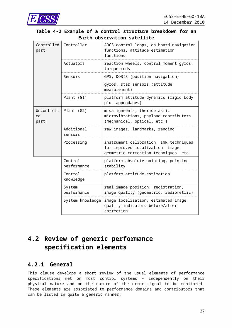
4.1.3 Example – Earth observation satelliteAs a typical illustration consider an Earth observation spacecraft, featuring a three-axis stabilised platform and an imaging payload. The platform is controlled by the AOCS to follow a given reference pointing profile (Nadir pointing, slow slew motion for example). A set of sensors monitors the attitude of the platform (gyros, star sensors for example) and feeds the on-board navigation (GPS for example); the AOCS control loops generate the appropriate commands for the actuators (reaction wheels, control moment gyros, magnetic torque rods...) so as to maintain the platform attitude close to the reference profile.Meanwhile the instrument is submitted to effects that cannot be controlled by the AOCS loops – such as misalignments, thermoelastic, microvibrations, payload distortions, etc. – that also affect the final system performance, and which can be in part identified and corrected on ground using additional information (such as image processing and landmarks identification).Table 4-2 maps this system to the extended structure of Figure 4-2:
21
ECSS-E-HB-60-10A14 December 2010
Table 4-2 Example of a control structure breakdown for an Earth observation satellite
Controlledpart
Controller AOCS control loops, on board navigation functions, attitude estimation functions
Actuators reaction wheels, control moment gyros, torque rods
Sensors GPS, DORIS (position navigation)gyros, star sensors (attitude measurement)
Plant (G1) platform attitude dynamics (rigid body plus appendages)
Uncontrolledpart
Plant (G2) misalignments, thermoelastic, microvibrations, payload contributors (mechanical, optical, etc.)
Additional sensors raw images, landmarks, rangingProcessing instrument calibration, INR techniques for
improved localization, image geometric correction techniques, etc.
Control performance
platform absolute pointing, pointing stability
Control knowledge platform attitude estimation System performance
real image position, registration, image quality (geometric, radiometric)
System knowledge image localization, estimated image quality indicators before/after correction
4.2 Review of generic performance specification elements
4.2.1 GeneralThis clause develops a short review of the usual elements of performance specifications met on most control systems – independently on their physical nature and on the nature of the error signal to be monitored. These elements are associated to performance domains and contributors that can be listed in quite a generic manner:
extrinsic performance elements: performance in steady state (converged) conditions, expressed in time or frequency domains; performance with respect to transient events intrinsic performance elements, mainly – but not exclusively – for closed-loop controlled systems, focused on the properties of the feedback loops (e.g. stability, stability margins, robustness, noise rejection).
22
ECSS-E-HB-60-10A14 December 2010
4.2.2 Preliminary remark on intrinsic and extrinsic performance properties
It is important to make a distinction between intrinsic and extrinsic properties. As stated by the corresponding definitions in clause 3,
“extrinsic” corresponds to those properties that depend on the interaction between the system and the exterior conditions, “intrinsic” corresponds to those properties that do not depend on this interaction.
From these definitions it appears clearly that a control error – say, an absolute pointing error – is a performance indicator belonging to the “extrinsic” category, whereas a stability margin – say, a gain margin – belongs to the “intrinsic” one.A natural consequence is that assessing extrinsic performances requires quantified hypotheses on the system environment (in practice, control reference, measurement noise level, disturbance amplitude), whereas assessing intrinsic performances does not.Generally the distinction is clear, but sometimes some ambiguity can arise – often due to the fact that a same word covers two different meanings. This is why for instance it is important to introduce a distinction between signal stability (extrinsic) and system stability (intrinsic), which physically describe two very different properties. The same kind of confusion can occur for terms such as “overshoot”, which according to the context can be understood as the maximum magnitude of a closed-loop transfer function (intrinsic property), or as the peak response of a system submitted to a step, an impulse or more generally a transient input or disturbance (extrinsic property).It is not intended in this document to redefine these possibly misleading terms in order to avoid ambiguity. Most of the control engineering wording is so well established that there is no way it can be changed. It is important that the requirement is clear and explicit enough when using a possibly ambiguous term so that the interpretation makes no doubt to the recipient.
NOTE In some exceptional situations the separation between extrinsic and intrinsic can be hardly applicable. This is the case for example for very non linear systems, whose system stability properties can be dependent on the current operating point.
For all control systems developed as part of a space project, the control performance requirements cover both extrinsic and intrinsic properties. To illustrate this, Table 4-3 gives an example of specifiable properties for the case of an AOCS loop:
Table 4-3 Example of AOCS extrinsic and intrinsic specifiable performances
Extrinsic performance properties
Intrinsic performance properties
Steady state properties
absolute pointing error, pointing stability, absolute measurement error, etc.
measurement noise transmission, rejection of external torque disturbances
Transient properties
attitude overshoot (entering a thruster control mode), tranquillization time (end of thruster control mode, rate reduction mode), etc.
overshoot, response time, settling time, damping, logarithmic decay etc.
General properties
fuel consumption, average solar array illumination, etc.
system stability, stability margins, robustness
23
ECSS-E-HB-60-10A14 December 2010
The intrinsic properties are – completely and exclusively – design dependent. They are fully determined by the quality of the design, independently on the nature of the environment. For instance correct stability margins, reduced closed-loop overshoot etc. are important indicators of the healthiness of the control tuning. Strictly speaking specifying most of these properties is relevant to “control design rules” more than to “control performance”. Nevertheless for pragmatic reasons (i.e. considering the way control performances are specified in practice on real projects) these questions are addressed in this “control performance” document rather than in a separate one about “control design rules”.
4.2.3 Examples of high-level performance requirements
4.2.3.1 GeneralIn practice many high-level performance requirements are expressed in very similar terms whatever the physical nature of the control system.
4.2.3.2 About steady state performance
4.2.3.2.1 OverviewIn steady state the performance generally quantifies the ability of the system to achieve properly the control reference in spite of internal and external disturbances, measurement noise etc. The reference can be either fixed (maintain a temperature to a given value for example) or varying along time (tracking system, slew profile for example).
4.2.3.2.2 Time domain requirementsThe needs can be expressed in time domain. The time domain performance specifications can deal with different temporal scales of the error signal (which can usually be seen as the difference between the reference and the actual states):
systematic error or bias component, long term drift, repeatability error after a given time period, short term signal stability over given time frames.
The associated requirements can be formulated in terms of deterministic definitions. For example:
maximum absolute pointing error in converged conditions < 0.1° minimum Sun avoidance angle in converged conditions > 30°
statistic definitions (mathematical expectation, standard deviation, Allan variance, etc.). For example,
pointing variation over a 5 s sliding time frame < 10 µrad 3
RMS value of the rate measurement error < 0.1°/sNOTE All the examples (and figures) given in this clause and the following ones are for illustration only. None of them correspond to an identified, real mission.
24
ECSS-E-HB-60-10A14 December 2010
4.2.3.2.3 Frequency domain requirements
The performance specifications in steady state can be also expressed in frequency domain (needs generally formulated in terms of PSD envelope).For example consider a drag-free satellite with a high sensitivity accelerometer. In converged science mode a specification is formulated stating that
“The PSD of the residual acceleration experienced at accelerometer level shall remain below a given envelope”.
4.2.3.2.4 Mixed time and frequency domain requirementsMixed time and frequency domains specifications can also be met.
NOTE For example: “The following two conditions shall be met:1. PSD of the error signal remains below a given envelope,
and 2. the temporal extrema is smaller than a given value.”
4.2.3.3 About transient performance The performances during transient situations are usually handled by a distinct set of relaxed requirements, considering that the behaviour is locally more disturbed than in converged steady-state situations – as far as these events are short and exceptional. Such transient situations can be met in practice at system initialisation, during a switch between two control modes, or after a discontinuity of the guidance profile – for example. The needs in transient situations are generally expressed in time domain:
overshoot (in the extrinsic sense, that means peak temporal response triggered by the transient event).
NOTE For example (on a telecom satellite in station keeping), “The maximum overshoot in pitch/roll shall be <0.1°.”
tranquillisation time (time required after transient triggering to return to converged conditions).
NOTE 1 For example (on an agile observation satellite), “The short term line-of-sight angular stability shall be back < 1 µrad in less than 10 s after the end of the worst case manoeuvre.” NOTE 2 Transient performances are generally expressed in time domain. Formulating transient requirements in frequency domain, or in time/frequency domain, is exceptional.
Some performance requirements in transient situations can also be expressed in terms of intrinsic properties of the system (that means, independently on the external conditions):
overshoot, here defined as the peak value of the closed-loop transfer function in frequency domain, mainly for closed-loop control systems (see Clause 4.2.2 on the possible ambiguities on the usual terms), response time, damping ratio, exponential decay, etc.
These properties are defined in clause 6 for linear time invariant systems.
25
ECSS-E-HB-60-10A14 December 2010
4.2.3.4 Other types of performance requirementsOther types of performance requirements can also be met that do not belong to the “steady state” nor “transient” categories, properly speaking. Some of them are rather generic and can be met in many different situations; for example:
Final state, final positioning accuracy, total consumption during a given phase (fuel, battery power), total duration of a given phase
Some are much more specific, associated to a particular type of application and of requirement. Taking some examples from spacecraft engineering:
number and statistics of thrusters firings, average illumination of the solar array during initial acquisition, number of occurrences of zero-crossing for a reaction wheel, number of cycles at low speed
There is an almost unlimited number of similar customised requirements that can be imagined, according to the nature of the control system of interest. A detailed analysis is out of the scope of this document; nevertheless the methods, rules and recommendations further developed in the next clauses are also helpful to formalise and analyse these problems.
4.2.4 Formalising requirements through performance indicators
4.2.4.1 GeneralClause 4.2.3 gives a (non exhaustive) list of usual high-level performance requirements that can be met on a large number of control systems. To be made applicable in practice these requirements are formalised so as to avoid any ambiguity or erroneous interpretation. This formalisation requires a set of mathematically well-defined performance indicators.
4.2.4.2 Extrinsic performance indicatorsThese indicators aim at quantifying the end-to-end behaviour of the control system submitted to environmental and measurement disturbances. As a consequence they are defined as one or several temporal or frequency properties of the separation between the true and the desired state(s) of interest.A quite general template for building such extrinsic performance indicators is given on Table 4-4.
NOTE 1 The formalism introduced above is indeed very general and allows handling a large variety of problems. There is no limit in theory to the number of possible error functions, operators, and properties to be verified, according to the nature of the control system and to the type of performance to be verified. NOTE 2 Nevertheless in practice most of the usual needs can be covered by a limited set of such error functions, operators and performance properties. For more details on how to define and to manage a separation function, for detailed definition of usual performance indices, and for guidelines on how to use them to formalise different types of requirements, refer to clause 5 of this document.
26
ECSS-E-HB-60-10A14 December 2010
NOTE 3 In all cases these performances are related to a consistent set of hypotheses for what concerns the environment disturbances, the measurement disturbances, and all the system parameters in a very wide sense. It is important that a performance requirement (as well as a performance verification) states very clearly to which set of hypotheses it refers.
Table 4-4 General template for building extrinsic performance indicators
Step #
Step description
Step 1 Identify the state (or states) of interest for the performanceNOTE: Euler angles for satellite AOCS performances, centre of mass position
for launcher GNC, temperature value for thermal control, etcStep 2 Define the error function (or functions): in a very general sense this is simply a
mathematical function which quantifies the relevant difference between two state elements or vectors.NOTE: algebraic difference (for scalar signals), distance, angular distance,
norm of vector difference, etcStep 3 Define the operator applying to the error function (if any)
NOTE: raw error value, sliding average, peak-to-valley variation over a sliding time interval of given duration, etc
Step 4 Define the performance properties to be verified: these properties can be either deterministic (e.g. maximum value), or statistical (e.g. 3σ value), or expressed in frequency domain (e.g. PSD below a given frequency envelope).
For illustration this is how the general process of Table 4-4 can be declined in the particular case of the roll pointing stability of a satellite:
State of interest: roll angle Separation function: algebraic difference between actual and desired roll angles Operator: peak-to-peak variation over sliding time frames of 5 s duration Statistical property: 3 value over a given mission scenario
4.2.4.3 Intrinsic performance indicatorsBuilding intrinsic performance indicators relies on a different process, since by definition such performances do not depend on the end-to-end temporal behaviour of the system, and are not a function of the state vector.The most usual intrinsic performance indicators for closed-loop control systems are (see also Table 4-3)
the stability margins, which require to be carefully defined according to the nature and the complexity of the system, the transient response properties such as overshoot and damping ratio, possibly some relevant frequency domain properties
27
ECSS-E-HB-60-10A14 December 2010
Other indicators can also be of interest, such as (for example) the convergence domain of a controlled system (envelope of initial conditions for which the system converges towards the desired equilibrium point).Refer to clause 6 of this document for more material on how to define, handle and specify the usual intrinsic performance indicators for closed-loop control systems.
4.3 Overview on performance specification and verification process
4.3.1 IntroductionPerformance specification and verification is a sub-process of the overall control engineering process described in [ECSS-E-HB-60A]. This clause presents an overview of the control performance management and verification process, covering all stages involved during the lifecycle of a typical space project.The overall process naturally divides into two areas:a. Requirements capture and dissemination.b. Performance verification.These are discussed in clauses 4.3.2 and 4.3.3 respectively. Typically these tasks are not performed sequentially: the results of the performance verification can lead to a change to the requirements dissemination and their subsequent re-verification. Several iterations can be needed to achieve a satisfactory performance budget which meets all top level requirements.Clause 4.3.4 explicitly defines the various tasks required for managing a control performance budget, and the responsibilities of the various parties involved for carrying out these tasks. It should be emphasised that different missions will have different structure and organisation: the discussions in this clause are for a general mission profile. This can need to be appropriately adapted for a particular mission.
28
ECSS-E-HB-60-10A14 December 2010
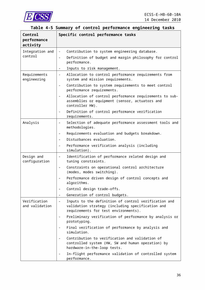
Table 4-5 Summary of control performance engineering tasksControl performance activity
Specific control performance tasks
Integration and control
- Contribution to system engineering database.- Definition of budget and margin philosophy for control
performance.- Inputs to risk management.
Requirements engineering
- Allocation to control performance requirements from system and mission requirements.
- Contribution to system requirements to meet control performance requirements.
- Allocation of control performance requirements to sub-assemblies or equipment (sensor, actuators and controller HW).
- Definition of control performance verification requirements.Analysis - Selection of adequate performance assessment tools and
methodologies.- Requirements evaluation and budgets breakdown.- Disturbances evaluation.- Performance verification analysis (including simulation).
Design and configuration
- Identification of performance related design and tuning constraints.
- Constraints on operational control architecture (modes, modes switching).
- Performance driven design of control concepts and algorithms.- Control design trade-offs.- Generation of control budgets.
Verification and validation
- Inputs to the definition of control verification and validation strategy (including specification and requirements for test environments).
- Preliminary verification of performance by analysis or prototyping.
- Final verification of performance by analysis and simulation.- Contribution to verification and validation of controlled system
(HW, SW and human operation) by hardware-in-the-loop tests.- In-flight performance validation of controlled system
performance.
4.3.2 Requirements capture & disseminationTypically, this process consists of the following stages:c. The mission objectives are used to derive a set of system level performance
requirements. These are generated by the top level customer or end user. These captured system level requirements are then placed on the mission prime contractor.
d. Then, the prime contractor divides the system level performance requirements appropriately, to produce requirements on the subsystems and on the equipment
29
ECSS-E-HB-60-10A14 December 2010
(sensors, actuators, control HW) such that if these requirements are met the system level requirements are also met.
e. This is repeated at lower level, such that each subsystem supplier also generates lower level performance requirements for their subcontractors (for example down to unit level).
This process is illustrated in Figure 4-3. The requirements management is a top-down process, consisting of an initial requirements capture task at top level, followed by requirements dissemination at each lower level of the process.The top-level requirements capture is generally performed at the start of development and then left unchanged. There can be exceptions to this: for example if the payload design is changed during development it can be necessary to modify the requirements accordingly. Requirements dissemination can need to be changed several times during development, depending on the outcome of the performance verification at each level.
4.3.3 Performance verificationAt each level in the process, performance are verified against the appropriate requirements. The overall verification is a bottom-up process consisting of the following activities:f. At the lowest requirement level in the tree, the performance of the appropriate
part of the system is calculated via preparation of an error budget.g. At higher levels, budgets are prepared by incorporating the budgets from lower
levels, together with errors intrinsic to that level.Thus, at all levels, the basic verification task consists of preparing a control error budget for that system or subsystem.As the project matures, more information becomes available for incorporation into the error budgets. In later phases, when components have been built, it can be possible to obtain information on the errors directly from measurement.
30
ECSS-E-HB-60-10A14 December 2010
Figure 4-3Example of requirements capture and dissemination for a typical AOCS case
Figure 4-4Example of pointing performance verification, for a typical mission profile
31
ECSS-E-HB-60-10A14 December 2010
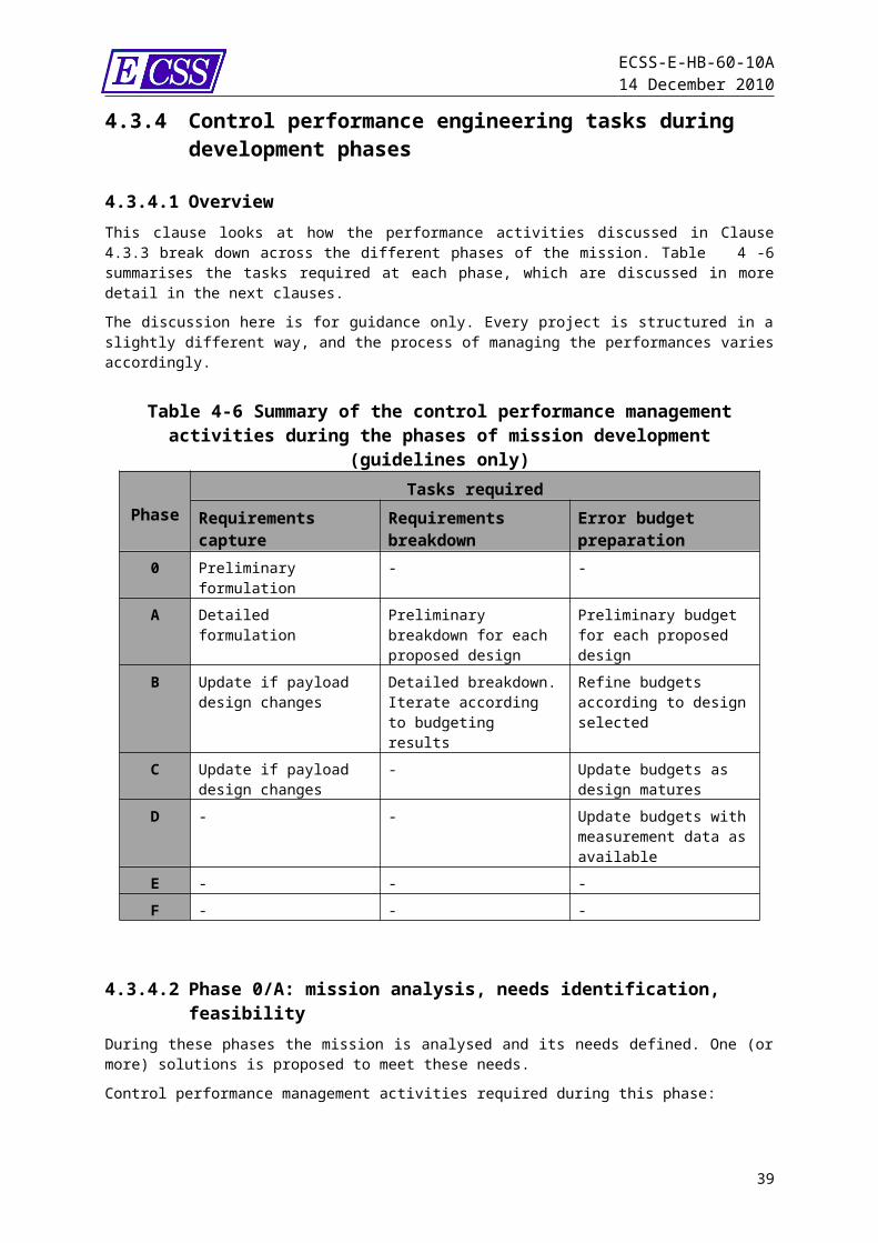
4.3.4 Control performance engineering tasks during development phases
4.3.4.1 OverviewThis clause looks at how the performance activities discussed in Clause 4.3.3 break down across the different phases of the mission. Table 4-6 summarises the tasks required at each phase, which are discussed in more detail in the next clauses.The discussion here is for guidance only. Every project is structured in a slightly different way, and the process of managing the performances varies accordingly.
Table 4-6 Summary of the control performance management activities during the phases of mission development (guidelines
only)
PhaseTasks required
Requirements capture
Requirements breakdown
Error budget preparation
0 Preliminary formulation
- -
A Detailed formulation Preliminary breakdown for each proposed design
Preliminary budget for each proposed design
B Update if payload design changes
Detailed breakdown. Iterate according to budgeting results
Refine budgets according to design selected
C Update if payload design changes
- Update budgets as design matures
D - - Update budgets with measurement data as available
E - - -F - - -
4.3.4.2 Phase 0/A: mission analysis, needs identification, feasibilityDuring these phases the mission is analysed and its needs defined. One (or more) solutions is proposed to meet these needs.Control performance management activities required during this phase:
Requirements capture: preliminary then detailed formulation of system requirements performed by the end user or top-level customer. These are the requirements to be met by the payload in order to perform the mission successfully. Requirements breakdown: a preliminary breakdown of requirements into subsystems, made by the top-level customer. These are used to provide performance requirements on the subsystem suppliers.If more than one design has been proposed, this applies to each design. The results of the error budget preparation can lead to an update of the requirements breakdown.
32
ECSS-E-HB-60-10A14 December 2010
Error budget preparation: Preliminary error budgets should be made for each of the subsystems, and hence for the system.If more than one design has been proposed, this applies for each option. In this case it is important that the budgeting is prepared in sufficient detail to allow the alternatives to be compared.
At the end of phase A the feasibility is established and a preferred approach is identified. It should be ensured that the proposed approach is able to meet the performance requirements identified.
Table 4-7 Control performance engineering inputs, tasks and outputs, Phase 0/A
0/A Requirements engineering
Analysis Design and configuration
Verification and validation
Inputs System objectivesMission requirementsSystem performance requirements
Controlled system performance objectivesPreliminary control system requirements
Control system design concepts of similar space systems
System verification and validation approach
Tasks Translate mission and system objectives into preliminary control performance needsPreliminary breakdown of performance requirements to sub-assemblies and equipment (sensors, actuators, and controller HW)
Preliminary disturbances evaluationAnalysis of control performance requirements feasibility & control system alternativesPreliminary performance assessmentInitial sensitivity analysisIdentification of performance critical aspects
Establishment and trade-off of control system design concepts
Control engineering support for definition of performance verification and validation conceptsPreliminary definition of control performance verification and validation methods and strategies
Outputs
Inputs to system requirements documentation
Control performance analysesInputs to Phase A system performance budgets
Performance criteria for selection of a preliminary baseline control system design
Inputs to development and verification plan & planning
4.3.4.3 Phase B: preliminary definitionThis phase covers the refinement of the selected solution to a coherent level. The control performance management tasks during this phase are:
Requirements capture: the requirements identified in phases 0/A should be refined where necessary.
33
ECSS-E-HB-60-10A14 December 2010
NOTE Although the generic requirements for the mission previously identified should remain the same, platform requirements can need to change according to payload design. For example for an imaging payload, the required pointing stability can be determined by the pixel size or imaging time, both of which can change as the payload design evolves.
Requirements breakdown: the top level requirements should be distributed to suppliers in the form of subsystem requirements. These can in turn be broken down into requirements on lower level suppliers.
NOTE The requirements breakdown can need to be iterated several times to achieve a satisfactory allocation, depending on the results of the error budget preparation.
Error budget preparation: the error budgets for each subsystem (and below where necessary) are assessed in as much detail as is possible at this stage. The aim is to confirm the feasibility of the adopted approach, identify any areas where margins are tight, and to provide information for use in deciding how to proceed with the design
NOTE The types of inputs which can be used at this phase are: comparison with previous missions, manufacturers information, analytical or a-priori models, etc
It is assumed that at the end of phase B there is a stable baseline for the design, with verifiable requirements established.
34
ECSS-E-HB-60-10A14 December 2010
Table 4-8 Control performance engineering inputs, tasks and outputs, Phase B
B Requirements engineering
Analysis Design and configuration
Verification and validation
Inputs System objectivesMission requirementsControlled system objectives and performance requirements
Phase 0/A simulation modelsPhase 0/A control analyses
Phase 0/A control design
System verification planPhase 0/A control verification plan
Tasks Generate controlled system performance requirementsDetailed breakdown of performance requirements to sub-assemblies and equipment (sensors, actuators, and controller HW)
Assessment of disturbances and other performance contributorsControlled system performance analysis Controlled system sensitivity analysisAnalysis of control performance constraints induced on sub-systems and components
Identify performance constraints for the preliminary design of control lawsDefinition of control system baselineEstablishment of control related budgets and margins
Contribution to preparation of controlled system verification planProvide inputs to lower level verification plans
Outputs
Inputs to system requirements documentation
Inputs to controlled system analysis report
Inputs to control system design report (including design justification from a performance point of view)Preliminary control performance budgets
Inputs to development and verification plan & planning
4.3.4.4 Phase C/D: detailed definition, production and ground qualification testing
Phase C involve detailed study of the solution identified in the previous stage, and covers all remaining activities relating to the mission design. Phase D comprises the manufacture and qualification testing. The control performance management tasks during these phases are:
Requirements capture: no significant changes to the performance requirements should be made after the PDR at the end of phase B. Minor changes can be needed to reflect modifications to payload design: these should have no significant impact on the design activities.
35
ECSS-E-HB-60-10A14 December 2010
Requirements breakdown: this should be updated as the design evolves. Ideally the fewest possible changes should be made to the requirements breakdown, however improved knowledge of the error budgets at all levels can require a reallocation of requirements to be made. Error budget preparation: the error budgets at each level prepared at phase B are refined as the design evolves.
NOTE 1 During phase C, the components to be used should be selected, the functional modes analysed, etc. The information used to produce the performance budgets should therefore come to more accurately reflect the actual system behaviour. NOTE 2 In addition to providing an updated budget at the end of this phase, it is recommended that the budgets are continually updated throughout the phase, with new or updated data being incorporated as soon as available. This should ensure that any potential problems are identified as early as possible, and not at the end of the phase when the design is supposed to be finalised.NOTE 3 As each component and subsystem becomes available and is tested, any actual measurements should be incorporated into the error budget to give a more realistic assessment of the actual errors for the actual SC.NOTE 4 In the case of systematic errors (biases, misalignments, etc.) earlier budgets should have assumed a range of possible values. Measurements on the actual equipment should allow an assessment of the actual error, with only measurement errors leaving any uncertainly.NOTE 5 For other error sources, such as sensor noise, it is not possible to obtain an actual value for the error, but repeated measurements should allow more accurate assessment of the error distribution to be made.
It is assumed that at the end of phase C the final design has been established, and it has been confirmed that each component and subsystem meet their performance requirements and that sufficient margins for uncertainty have been established.At the end of phase D, the production activities end. At this point it is very important that the end user or top level customer ensures that, given the current knowledge of the errors, all performance requirements are in the conditions of the mission.
36
ECSS-E-HB-60-10A14 December 2010
Table 4-9 Control performance engineering inputs, tasks and outputs, Phase C/D
C/D Requirements engineering
Analysis Design and configuration
Verification and validation
Inputs Phase B control objectives and requirementsPhase B control components specification
Phase B simulation modelsPhase B control analyses
Phase B control design and design justification
Phase B controlled system verification plan
Tasks Update of performance specificationsReview and assessment of control performance requirements changes
Detailed controlled system performance analysisUpdate of sensitivity analysisSupport to performance verification processSupport to definition of in-flight performance verification process
Detailed design of controllers and optimisation of controller parametersReview of control performance budget and margins analysisDetailed design and tuning of control-related FDIR
Provide inputs and verify consistency with higher level controlled system verification activitiesMonitor lower level verification acceptance activitiesMonitor lower level qualification and acceptance tests (e.g. at sensors/actuators level)
Outputs
Updated inputs to system or subsystem technical specificationsUpdated inputs to lower level technical specifications and to ICDs
Final controlled system analysis report (performance clauses)Inputs to the definition of the strategies for the in-flight calibration and performance analysis
Final control system design report – Justification of performance related featuresFinal control system performance budgets
Contribution to controlled system verification reportInputs to in-flight verification plan
4.3.4.5 Phase E/F: utilisation and disposalThese phases cover the launch and operation of the mission, and all events from end of life until final disposal of the product. The control performance management tasks during these phases consist of supporting the IOT, the calibration activities, and – if any – all specific development needed to ensure a proper disposal (for example in the event of the reorbitation of a telecommunications satellite at end of life).
NOTE It is recommended to summarise all lessons learnt from the error management of the mission, for example whether assumptions made during the early phases were shown to be valid during manufacture and
37
ECSS-E-HB-60-10A14 December 2010
testing. Such information can be used to benefit future missions.
Table 4-10Control performance engineering inputs, tasks and outputs, Phase E/F
E/F Requirements engineering
Analysis Design and configuration
Verification and validation
Inputs Final system and lower level specification
Controlled system requirementsControlled system in-flight performance dataStrategies for the in-flight performance analysis
Final control system design report
In-flight verification plan
Tasks Comparison of in-flight performance with control objectives and requirementsClarify control objectives and requirements changes during operation
Support and analysis of relevant calibration operations (if any)Analysis of controlled system operational performanceAnalysis of required controller changes (if any) and identify performance impacts
Identify control performance constraints applicable to control design updates (if required)
Support controlled system operational performance verification
Outputs
New control performance related operational requirements
Inputs to controlled system operational performance reportInputs to updated controlled system analysis reportInputs to payload data evaluation
Controller design updates (updated control system design report)
Inputs to in-flight acceptance reviewInputs to periodic mission reports
38
ECSS-E-HB-60-10A14 December 2010
5Extrinsic performance – error indices and
analysis methods
5.1 IntroductionThis chapter considers aspects related to steady-state or transient extrinsic performance of a general control system; basically it handles “signals” (states or outputs) in time domain. Its purpose is to develop the formalisation process outlined in clause 4.2.4.2 by carefully defining error functions and error indices, and by describing how to formulate a performance requirement using these indices. It also addresses the methods to be used for assessing compliance with a performance requirement and to build up a performance budget.
NOTE For similar considerations on intrinsic performance properties, refer to clause 6 of this document.
5.2 Performance and measurement error indices
5.2.1 Definition of error functionA performance error is some function quantifying the difference between the actual state of a system and its desired state:
Similarly, a knowledge error is a function quantifying the difference between the estimated (or known) state of the system, and the actual state:
It is not possible to give a simple prescription for the choice of this function. The exact definition of function is system dependent and decided based on the appropriate quantities of interest.
NOTE 1 For example, if the interest is in the attitude of a spacecraft with respect to a target orientation, then the obvious choice of error function is the Euler angles from the target body (or payload) frame to the actual body (or
39

ECSS-E-HB-60-10A14 December 2010
payload) frame, or for knowledge errors between the estimated and actual frames:
,
NOTE 2 For example, alternatively, if the interest lies in orientating some vector (such as a payload line of sight) in a given direction, then the most appropriate choice of function is the angle between vectors:
,
NOTE 3 It can also be possible that several different functions are required for a single mission.
5.2.2 Definition of error indicesGenerally the performance and knowledge error functions defined in 5.2.1 are not static quantities, but have a complicated behaviour in the time domain. An error index is a way of capturing the particular feature of the variation which is of interest. Formally, a performance error index is a mathematical operator applied to the error function between actual and desired statesSimilarly, a knowledge error index is an operator applied to the separation function between the estimated (“known”) and actual states. Less formally, an index consists of simple functions (instantaneous value, time average) applied to the time signal of the error.
NOTE 1 All error indices considered here are the sums of time averages of a signal. This is because such indices applied to a linear sum of errors preserve the linear relationship: see clause 5.5.4 and annex .NOTE 2 Although only time-varying errors are described here, as this is the most common case, it is also possible to have situations in which the error varies according to another quantity, for example position on the sky. Annex B.1 discusses how to adapt the error index formalism to this case.
Clauses 5.2.3 and 5.2.4 define the most commonly used error indices. The use of these indices is for describing performance and knowledge errors, as experience has shown that common terms such as ‘stability’ can have different meanings to different users (see annex B.3). Other error indices can be defined similarly if required for a particular system or mission.
5.2.3 Common performance error indices
5.2.3.1 Absolute performance error (APE)The APE is defined as the instantaneous value of the performance error at any given time:
40
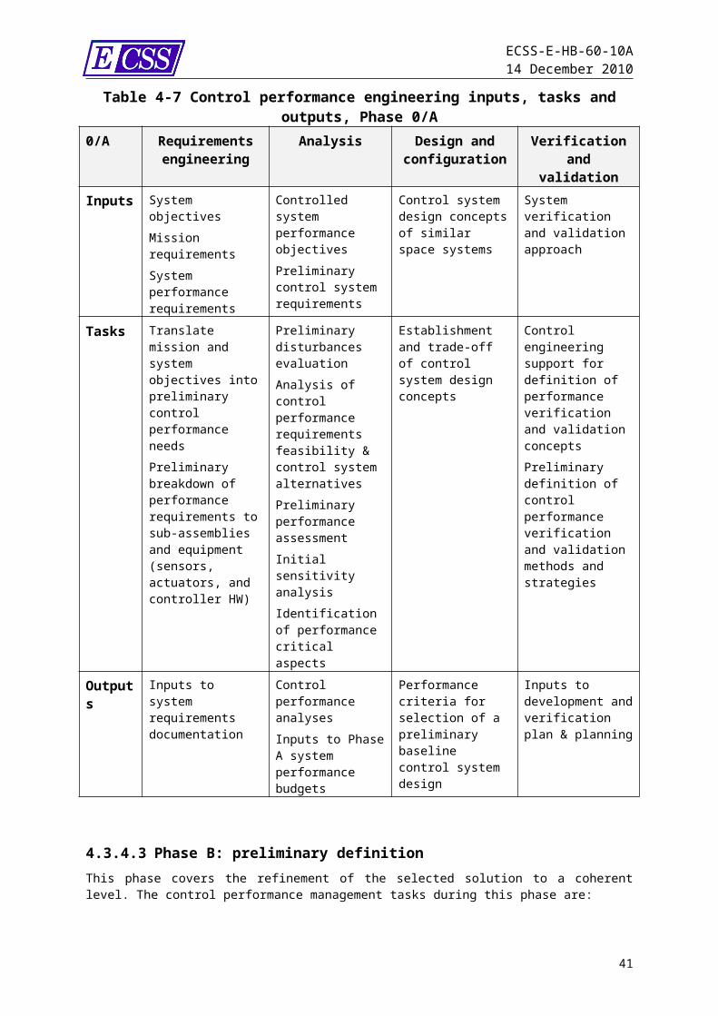
ECSS-E-HB-60-10A14 December 2010
5.2.3.2 Mean performance error (MPE)The MPE is defined as the mean value of the performance error over a specified time interval:
NOTE See annex B.2 for discussion of how to specify the interval t.
5.2.3.3 Relative performance error (RPE)The RPE is defined as the difference between the instantaneous performance error at a given time, and its mean value over a time interval containing that time:
NOTE as stated here the exact relationship between t and t is not well defined. Depending on the system it can be appropriate to specify it more precisely: e.g. t is randomly chosen within t, or t is at the end of t. See annex B.2 for further discussion
5.2.3.4 Performance stability error (PSE)The PSE is defined as the difference between the instantaneous performance error at a given time t and the error value at an earlier time t-t
NOTE The time t is fixed, with the choice of value being determined by the payload requirements
5.2.3.5 Performance drift error (PDE)The PDE is defined as the difference between the means of the performance error taken over two time intervals within a single observation period:
Where the time intervals t1 and t2 are separated by a time interval tPDE. NOTE Ensure that the durations of t1 and t2 are sufficiently long to average out short term contributions. Ideally they have the same duration. See annex B.2 for further discussion of the choice of t1 , t2, tPDE.
5.2.3.6 Performance reproducibility error (PRE)The PRE is defined as the difference between the means of the performance error taken over two time intervals within different observation periods:
41
ECSS-E-HB-60-10A14 December 2010
Where the time intervals t1 and t2 are separated by a time interval tPRE. NOTE 1 Ensure that the durations of t1 and t2 are sufficiently long to average out short term contributions. Ideally they have the same duration. See annex B.2 for further discussion of the choice of t1 , t2, tPRE.NOTE 2 The mathematical definitions of the PDE and PRE indices are identical. The difference is in the use: PDE is used to quantify the drift in the performance error during a long observation, while PRE is used to quantify the accuracy to which it is possible to repeat an observation at a later time.
5.2.3.7 Other performance error indicesIt is possible to define other performance error indices if required for a particular project, e.g. as different combinations of time averages. If used, these should be clearly defined similarly to the performance indices specified in subclauses 5.2.3.1 to 5.2.3.6.
5.2.4 Common knowledge error indices
5.2.4.1 Absolute knowledge error (AKE)The AKE is defined as the instantaneous value of the knowledge error at any given time:
5.2.4.2 Mean knowledge error (MKE)The MKE is defined as the mean value of the knowledge error over a specified time interval:
NOTE See annex B.2 for discussion of how to specify the interval t.
5.2.4.3 Relative knowledge error (RKE)The RKE is defined as the difference between the instantaneous knowledge error at a given time, and its mean value over a time interval containing that time:
NOTE See annex B.2 for discussion of how to specify the interval t.
42
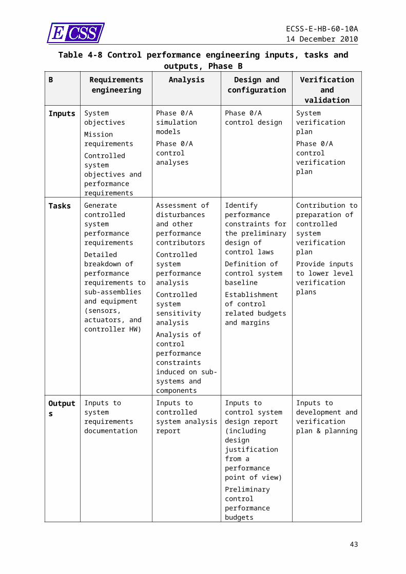
ECSS-E-HB-60-10A14 December 2010
5.2.4.4 Other knowledge error indicesIt is also possible to define further knowledge error indices, analogously to the case for performance error indices. These are not generally required and so are not explicitly stated here.
5.3 Formulation of performance requirements using error indices
5.3.1 Structure of a requirementA performance requirement for some system is expressed by giving an upper bound, Imax, for some quantity, expressed as an error index I(eP), together with a probability that the index lies within this bound. Expressed mathematically:
In order that the requirements are clear and unambiguous, it is important to ensure that the following elements are be present:h. The exact definition of the property to be constrained, which needs:
1. The choice of error function eP
2. The index to be applied to this function, I(eP)i. A maximum allowed value for this index, Imax.j. The required probability, PC, that the index is inside the allowed rangek. The conditions under which the probability is to apply (known as the “statistical
interpretation”)Guidelines as to how to define these elements are given in the next clauses.
NOTE 1 Although only performance requirements are discussed here, the same structure applies to measurement requirements, with some additional considerations discussed in 5.3.5.NOTE 2 A requirement is commonly expressed in words, for example:“The APE of the rotation about the x-axis shall be less than 5 arcsec (95% probability) using the temporal interpretation”. This is equivalent to the mathematical formulation above.
5.3.2 Choice of error functionAn error function is some quantity defining the difference between the true and demanded state. The function is chosen such as to capture the aspects of the difference between states which affects the system output.For example, when formulating attitude (pointing) requirements on a spacecraft, the important quantity is an angle or angles. Depending on the exact nature of the system this can be
the Euler angle(s) for the transformation from a coordinate frame representing the demanded attitude, to another frame representing the real attitude
43
ECSS-E-HB-60-10A14 December 2010
the angle between the direction of a payload boresight and the (inertially fixed) direction of the target
These are actually different ways of constraining the same system. The most appropriate one for the system under consideration is determined by engineering judgement.
NOTE Typically several different error functions are needed to capture different elements of the performance of a system.
5.3.3 Use of error indicesThe error function defined in 5.2 varies with time (or another domain variable). To place requirements on particular features of this variation, the signal error indices defined in clause 5.2.3 are used.l. The APE index is used for requirements on the instantaneous value of an errorm. The MPE index is used for requirements on the mean error over some periodn. The RPE index is used for requirements on the deviation from the meano. The PSE index is used for requirements on the change of error over a given timep. The PDE index is used for requirements on the change of the mean over timeq. The RPE index is used for requirements on the ability to repeat an observation at a
later timeBy appropriate choices of timescale and statistical interpretation, these indices can be tuned to capture many different features of the error variation, and hence to place requirements on these features. Annex B.2 and B.3 discusses this in more depth.
NOTE 1 The indices listed above are the most common error indices, if needed others can be defined to capture other aspects of behaviour.NOTE 2 Only errors which are a function of time are considered in the main text, as this is the most common case. For cases where the error is a function of another quantity see annex B.1.
5.3.4 Statistical interpretation of a requirement
5.3.4.1 IntroductionSince all performance requirements are framed in terms of probabilities, when giving a requirement it is necessary to specify how to deal with contributing uncertainties. This is commonly known as the “statistical interpretation” of the requirement. This concept needs some explanation. Suppose for example that we have a requirement prob(e < 1) > 0.9. That is:
“There shall be at least a 90% chance of the error having a value less than 1”. The error is a function of the time, t, and of a set of ensemble parameters (parameters defining the state of the system) A1, A2, … AN. These are not generally known exactly but each can be described by a probability distribution P(Ai).The requirement can be met in different ways. It can be that e < 1 for most (but not all) of the time irrespective of the choice of ensemble parameters. Alternatively, most possible choices of parameters can give e < 1 at all times, but a few sets of parameters can give e > 1. Depending on the real mission needs, it can happen that one of these is acceptable and the other is not.
44
ECSS-E-HB-60-10A14 December 2010
For example, it can happen that to an observation cannot be done unless e is less than 1 over the entire observation period. In this case, having a small fraction of cases with failed observations (e > 1) can be acceptable, but a situation in which all combinations of ensemble parameters gave e > 1 at some point during an observation, however briefly, can be unacceptable.
0 0.1 0.2 0.3 0.4 0.5 0.6 0.7 0.8 0.9 10
0.2
0.4
0.6
0.8
1
t
e P
0 0.1 0.2 0.3 0.4 0.5 0.6 0.7 0.8 0.9 10
0.2
0.4
0.6
0.8
1
t
e P
Figure 5-5 Illustration of the different ways of meeting a requirement.
0 0.1 0.2 0.3 0.4 0.5 0.6 0.7 0.8 0.9 1-10
-5
0
5
10
15
Time
Erro
r
-20 0 200
0.2
0.4
0 0.1 0.2 0.3 0.4 0.5 0.6 0.7 0.8 0.9 1-10
-5
0
5
10
15
Time
Erro
r
0 10 200
0.2
0.4
0 0.1 0.2 0.3 0.4 0.5 0.6 0.7 0.8 0.9 1-10
-5
0
5
10
15
-20 0 200
0.1
0.2
Figure 5-6Statistics for the different statistical interpretations. L-R: temporal interpretation, ensemble interpretation, mixed
interpretation
It is also possible to think of situations in which the ensemble parameters A1, A2, … AN
are not all treated identically. For example, we can say that a requirement applies to all possible values of the sensor biases, but only for only 99% of possible combinations of the other ensemble parameters.When formulating requirements, it is important to determine what really needs to be constrained, based on the payload needs. It is important then to make clear in the specification how to handle the statistics in order to avoid any possible confusions (that is, to specify the parameters to be set to the worst case, and the parameters to be integrated over the probability). Failure to be clear on this can result in an apparent compliance where there is a hidden non-compliance.The following subclauses define the most commonly used statistical interpretations.
5.3.4.2 Temporal interpretationFor this interpretation all time dependent variables are allowed to vary, but the time-independent ensemble parameters are set to worst case.
NOTE For example:“The requirement shall hold for 95% of the time for any possible spacecraft configuration.”
45
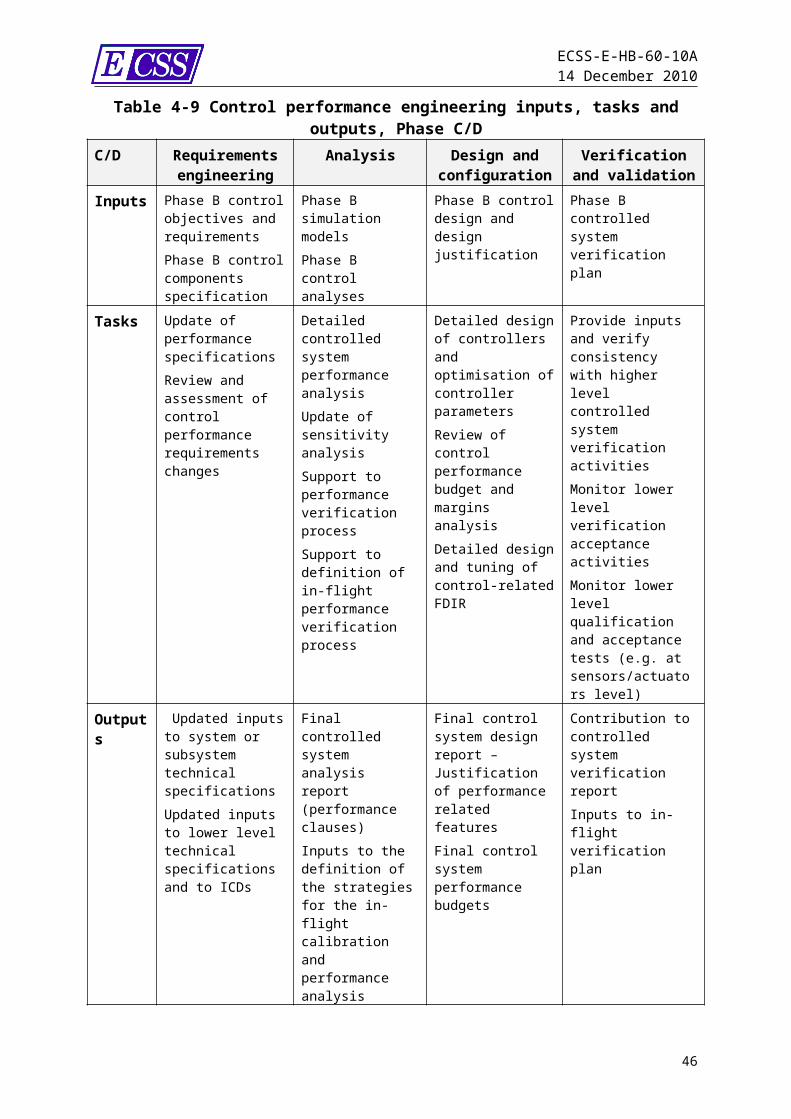
ECSS-E-HB-60-10A14 December 2010
This interpretation is used for requirements imposed to ensure that the spacecraft performs adequately, but where occasional short-duration holes of degraded performance are acceptable.
NOTE Since “any possible spacecraft configuration” potentially includes extreme cases, such a requirement can be difficult to verify. For this reason the modified statistical interpretation is preferred.
5.3.4.3 Modified Temporal Interpretation For this interpretation all time dependent variables are allowed to vary, but the time-independent ensemble parameters are set to worst case. However unlike the pure temporal interpretation extreme cases are explicitly excluded
NOTE For example:“The requirement shall hold for 95% of the time for any possible spacecraft configuration, except for configurations for which one or more ensemble parameters lie outside the 99.73% bound”.
5.3.4.4 Ensemble Interpretation For this interpretation all time dependent variables are set to their worst case value, but the ensemble (knowledge) parameters allowed to vary across their range.
NOTE For example:“This requirement shall hold at all times, for 95% of allowed spacecraft configurations ”
This interpretation is used for requirements on our knowledge of the SC. NOTE 1 For example:“a. The spacecraft pointing shall. fulfil the requirement 100% of the time for this mission to be a complete success.b. A 5% chance of the mission being only a partial success may be tolerated.NOTE: This is because of extreme biases, etc.”NOTE 2 In practice it is not usually appropriate to treat every single ensemble parameter in the same way. See subclause 5.3.4.7 (Other interpretations).
5.3.4.5 Mixed InterpretationAll variables, time dependent or ensemble, are allowed to vary.
NOTE 1 For example:“This requirement shall hold for 95% of allowed spacecraft configurations and times”.NOTE 2 A requirement of this form permits both of the scenarios shown in Figure 5-5. For this reason it should be used with care, and not as a ‘default’ statistical interpretation.
5.3.4.6 Modified Mixed InterpretationThis interpretation is similar to the mixed case but .
NOTE For example:
46
ECSS-E-HB-60-10A14 December 2010
“This requirement shall hold for 95% of the time for 95% of possible spacecraft configurations”
This is a weaker requirement than the ensemble or temporal interpretations as it allows both types of excursion, but with limits on both.
5.3.4.7 Other interpretationsOther statistical interpretations can be appropriate. It can be necessary to treat some ensemble parameters differently than others.
NOTE The following are two examples: “The requirement e < emax shall be met for 95% of possible orientations on the sky, for 100% of the time and 99% of allowed spacecraft configurations”. “The requirement e < emax shall be met 95% of the time, with all time-varying ensemble parameters set to end-of-life vales, for 100% of other ensemble parameter combinations”.
It is not possible to give a simple prescription for identifying the statistical interpretation, this is done individually based on what is appropriate for the system under consideration.
5.3.5 Formulation of Knowledge RequirementsThe previous discussion is formulated in terms of performance requirements, i.e. on differences between the real and desired states. Requirements on knowledge errors, i.e. on differences between the estimated and real states, are formulated analogously to performance requirements with the same issues arising, but with one extra consideration. When formulating knowledge requirements it is also necessary to specify for what state of knowledge the requirements apply. This can be
raw measurement data data available to a controller in (near) real time accuracy to which it is possible to reach using post-processing
It is important to make always clear which of these applies. It can be necessary to have different sets of requirements for different states of knowledge.
NOTE Typically requirements on on-board accuracy are driven by the need to meet performance requirements, while requirements on the post processing are independent and driven directly by mission needs.
5.4 Assessing compliance with a performance requirement
5.4.1 OverviewIn order to determine whether or not a system’s performance is compliant with a requirement, there are several methods which can be used:
1. experimental results
47
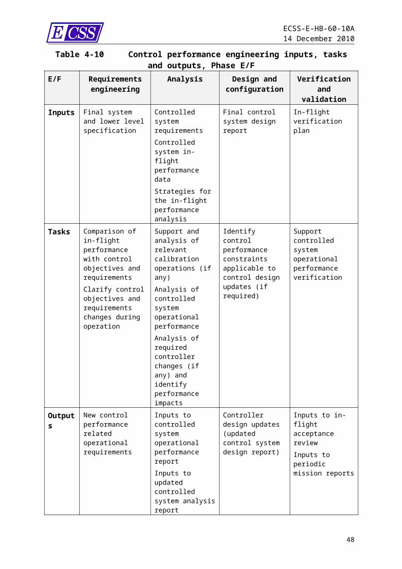
ECSS-E-HB-60-10A14 December 2010
2. numerical simulation3. compilation of a performance budget
Each of these is considered separately in 5.4.2, 5.4.3 and 5.5, with further details regarding performance budgets being given in 5.5.Some combination of each of these approaches should be used in a validation campaign, as each has strengths and weaknesses. Experimental validation can be the best verification, but can be impossible until a late stage in development. Numerical simulation allows verification of the system performance in a wide range of situations, but relies on the assumptions made to model the system. Budgeting can be performed from an early stage, but relies on realistic numerical values being available, and makes mathematical assumptions which can lead to an overly conservative estimate of performance.
5.4.2 Experimental approachAssessing compliance with a performance requirement based on an experimental approach has several advantages but also drawbacks and practical limitations which can make it insufficient or even unfeasible:
Advantages: verification based on real HW no need for models, statistical hypothesis, combination rules etc.
Drawbacks and limitations: some HW cannot be operated properly on-ground (effects of gravity for example) experimental approach can let statistical dispersions aside (test done on one given physical specimen, no way for changing its parameters)
In practice experimental approaches are well adapted to “simple” systems (equipment for example), which can be extensively characterised on-ground. In some cases there is no alternative solution (for example when using off-the-shelf elements, or subsystems provided by a subcontractor without detailed mathematical model).For complex systems (AOCS for example), there is no way an end-to-end test can be realistically run. Tests can be used to characterise some given elements of the system, and these experimental results feed the global verification process which is built up based on numerical simulations or analytical error budgets (see 5.4.3 and 5.4.4).
NOTE “Experimental approach” can also involve experience return (such as on-orbit return for satellites).
5.4.3 Numerical simulations
5.4.3.1 General considerationsThere are different ways in which simulations can be used to verify performance requirements:r. Simulations of specific cases, i.e. specified values for each parameter. The values
can be chosen on the basis ofs. expected typical values (nominal performance)t. identified worst case values to give worst case performances
48

ECSS-E-HB-60-10A14 December 2010
u. Multiple simulations covering different possible values of the parameters. This can consist of either
v. sweeping the parameter space to cover all possible valuesw. Monte Carlo techniques for sampling the parameter spacex. Mixing the two previous cases by setting some parameters to worst case or typical
values while doing multiple runs with different values of the other parametersThe choice of the appropriate simulation campaign depends upon the requirements to be assessed, in particular on the statistical interpretation. Simulation campaigns have limitations, as they can exclude some effects, and those effects which are included can misrepresent the reality
NOTE For example, fuel sloshing and structural vibrations are known to be difficult to incorporate into a realistic simulation
For this reason simulation campaigns should be used together with error budgeting, the error budget being used to show that including effects excluded from the simulation do not cause the system to become non compliant with the requirement.
5.4.3.2 Simulation of worst case scenariosIn many cases it is desirable to avoid a full Monte Carlo simulation campaign, usually because of the time it takes to perform and analyse. An alternative approach is to identify a few worst case scenarios, and simulate only these. Such an approach is appropriate for requirements to be met for all values of ensemble parameters, and for which a worst case can be clearly shown to exist.
NOTE 1 For example, if for a requirement to be met for all values of a sensor bias, it can be shown that the error increases with increasing bias, then it is not necessary to run simulations with all bias values, but only with the largest bias. NOTE 2 This is straightforward for a single parameter, but not for a large number of parameters interacting with each other.
If the approach of modelling only a few worst cases is adopted, it is important to clearly justify it, stating:y. why a low number of simulations is considered acceptablez. why the specific scenarios considered are the worst case onesThe probability of all ensemble parameters simultaneously having worst case values is extremely low. If the worst case scenario is simulated and the performance found to be non compliant with the requirement, then this does not necessarily mean that the system is non compliant. In this case it is recommended to perform further analysis, either analysing more realistic values or carrying out a Monte Carlo campaign to assess the probability of the system being compliant.
5.4.3.3 Monte Carlo simulation campaignsA Monte Carlo simulation campaign consists of a set of simulation runs each using different values of the parameters defining the statistical ensemble.
NOTE There is a large body of literature on Monte Carlo methods, this clause only covers the most basic relevant points.
Monte Carlo simulation campaigns should be used:
49
ECSS-E-HB-60-10A14 December 2010
If the requirement is imposed only for a specified fraction of the statistical ensemble If the parameter space involved is sufficiently large and complex that it is not possible to use analysis to determine a single worst case scenario to be simulated.
An appropriate verification of the compliance with the requirement cannot be performed if a sufficiently large number of simulation runs are not used. It is not possible to a-priori define the minimum number of runs required without making some assumptions. For a requirement specified with confidence level PC, the minimum number of runs required to verify that the requirement holds (to a verification confidence level of 95%), is given in Table 5-11. This table makes assumptions about how many actual cases of requirement violation (i.e. x > xmax) are seen.
NOTE “Requirement confidence level” is the probability level stated in the requirement, i.e. the required probability that x < xmax (with appropriate statistical interpretation). “Verification confidence level” is the confidence of the (unknown) true probability meeting the requirement given the experimental data available.
Table 5-11Minimum number of simulation runs required to verify a requirement at confidence level Pc to a verification confidence of
95 %Requirement confidence level PC
Minimum number of runs required for number of observed failures Nfail
Nfail=0 Nfail=1 Nfail=2 Nfail=368% 7 12 17 2195% 58 92 123 15299.73% 1108 1755 2329 2869NOTE 1: The derivation of these values is given in annex B.4NOTE 2: “Failure” in this context means violation of the specified bound, x > xmax.
5.4.4 Use of an error budgetFull details of the procedure of compiling an error budget are given in 5.5.Error budgeting consists of mathematical techniques for combining the (measured or estimated) uncertainties on the parameters affecting the system in order to estimate the total uncertainty of the system performance.The advantage of error budgeting is that it is relatively easy to do. The disadvantage is that the accuracy of the computed values is heavily dependent on both the input values and the assumptions made. Error budgeting should not be considered as being independent of validation by experiment or numerical simulation. Values from experimental or simulation results are used as inputs to the budgets, which allows effects which cannot be easily included in an experiment to be accounted for.
50
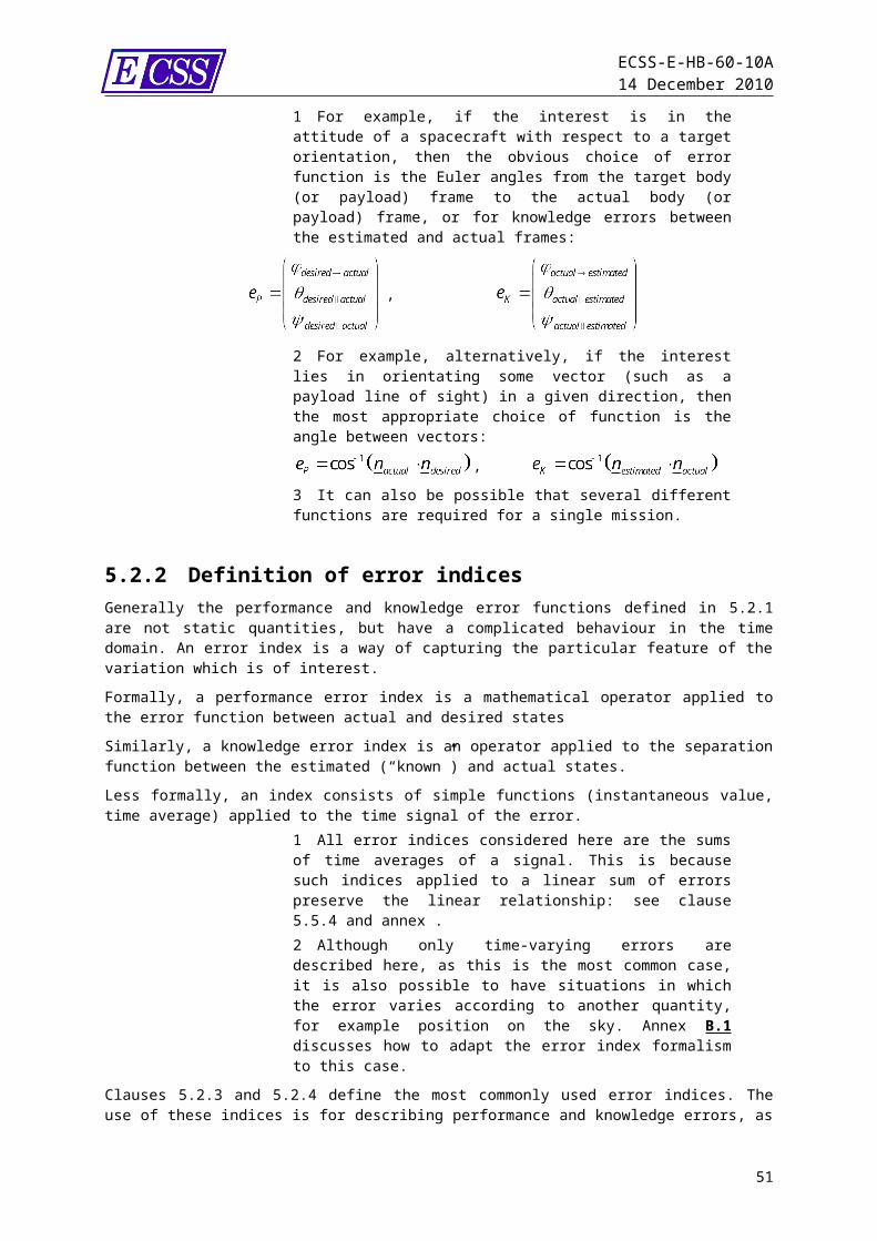
ECSS-E-HB-60-10A14 December 2010
5.5 Performance error budgeting
5.5.1 OverviewThis clause describes the process of verifying a requirement using an error budget. This consists of:
identifying the contributing error sources determining how they contribute to the total error determining or estimating the statistics of the contributing error sources combining these statistics to find the statistics of the total error, which can then be compared to the requirement
This is not a simple subject to deal with, as the underlying mathematics of probability distributions is complex, and although approximations can be used they are not always valid. This clause aims to keep the level of complexity down to the minimum required, but for an accurate budget some degree of complexity is unavoidable. Mathematical details not necessary for following the overall flow are given in appendices B.5 (assignment of PDFs to errors) and B.6 (combination of PDFs).
5.5.2 Identifying errorsThe first stage in compiling an error budget is to identify the contributing errors. It is not possible to give here a complete list of errors sources, as these depend upon the system. The worked examples in Annex C can be used as guidelines. Other points to be kept in mind when identifying contributors:All possible error sources should be considered, rather than a-priori assuming that some do not. Even non-dominant contributors can have a significant effect for some error indices.
NOTE For example, the contribution of a slow drift to the APE can be very low, and in this case it is possible to ignore it in the APE budget, but it can make a huge different to the PRE budget, which has fewer contributors.
The contributing error sources (1, 2, …, N) do not generally contribute equally to the total error, but need to be scaled by some factors (c1, c2, …, cN): eTotal= c1 1 + c2 2 + c3 3 +…+ cN N
NOTE 1 For example, if eTotal is the attitude error about an axis a, while the i’th contributing error i acts about an axis ai, then the scaling constant is be given by NOTE 2 In this clause, only linear sums of errors are considered: for example the sum of angular errors about an axis. NOTE 3 In the following clauses, the scale factors (c1, c2, …, cN) are assumed to be constant, that is they do not vary with time or as ensemble parameters.
51
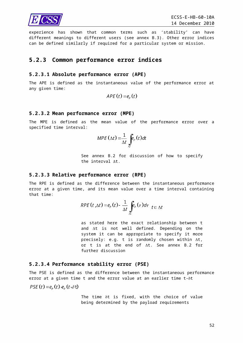
ECSS-E-HB-60-10A14 December 2010
5.5.3 Statistics of contributing terms
5.5.3.1To find the statistics of the total error, we first need accurate statistics for the individual errors contributing to it.
NOTE In this context, “individual error” refers to the time behaviour of the total performance error which occurs if no other sources of error are present
The main factors determining the assignment of a probability distribution (PDF) to an error are:aa. The temporal variation of that error (constant bias, random noise, periodic, etc.)bb. The error index (APE, MPE, RPE, etc) being assessedcc. The statistical interpretation of the requirement being assessed (see clause 5.3.4)dd. The amount of information available regarding the distributions of the ensemble
parameters
5.5.3.2Generally, the total error is obtained by approximate methods, which instead of combining the full PDFs of the error sources look only at their means and variances:
These can be obtained by various means:ee. In many cases it is possible to find the means and variances without computing the
full PDF. NOTE Data on sensor noise is typically provided in this form by the manufacturer, while the full PDF is not usually given.
ff. In other cases there are standard formulae for finding and : these are given in the relevant clause of Annex B.
gg. In many situations (especially if the “mixed” statistical interpretation is being applied) it is necessary to first obtain the PDF for an error, and then extract and .
Annex B.5 gives full details of how to assign PDFs to the individual errors based on these factors.
NOTE When finding values for the means and variances, it is important that they be estimated in a conservative way, since underestimating them can potentially give a “false compliance” when using a budget to see if the requirement is met. In particular, the method of identifying known maximum and minimum value with the 3 range of a Gaussian distribution, and hence estimating , underestimates the variance if the true shape of the distribution is non-Gaussian.
52
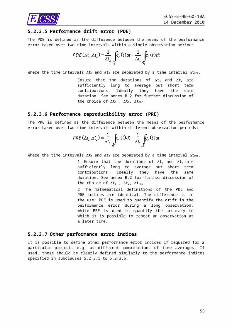
ECSS-E-HB-60-10A14 December 2010
Annex B.5 gives details of how to estimate the variance more accurate.
5.5.4 Combination of error termsGiven PDFs for each individual contributing error, the PDF for the total error can be obtained by combining them using the mathematics given in annex B.6. For all but the most trivial cases only a numerical approach can be done, either by direct integration or by Monte Carlo techniques. There is therefore a need for a simpler approximate assessment.Assuming that the total error is a linear sum of N contributing terms,
, then the combination approach recommended in this document is as follows:hh. The errors contributing to an index are grouped into nC classes, the details of the
grouping being dependant on the nature of the system being studiedNOTE See worked examples in annexes
ii. For each contributor to an index, the mean i and standard deviation i are obtained
NOTE See clause 5.5.2 and annex B.5.jj. the mean and standard deviation of the total errors in each of the classes are
computed using the following method:1. If it can be shown that the errors are not correlated, then the following
summation rules apply:
2. If it can be shown that the errors are correlated, or if there is reason to suppose that they can be correlated, then the following (more conservative) summation rules are applied
Where means that the summation is over all errors grouped in this class
kk. To find the mean and standard deviation of the total error, the means and standard deviations are summed as follows:
NOTE 1 The justification for this method is based on the fact that, for a linear sum of contributing terms, then applying one of the error indices defined in 5.2.3 and 5.2.4 preserves this linear relationship:
53
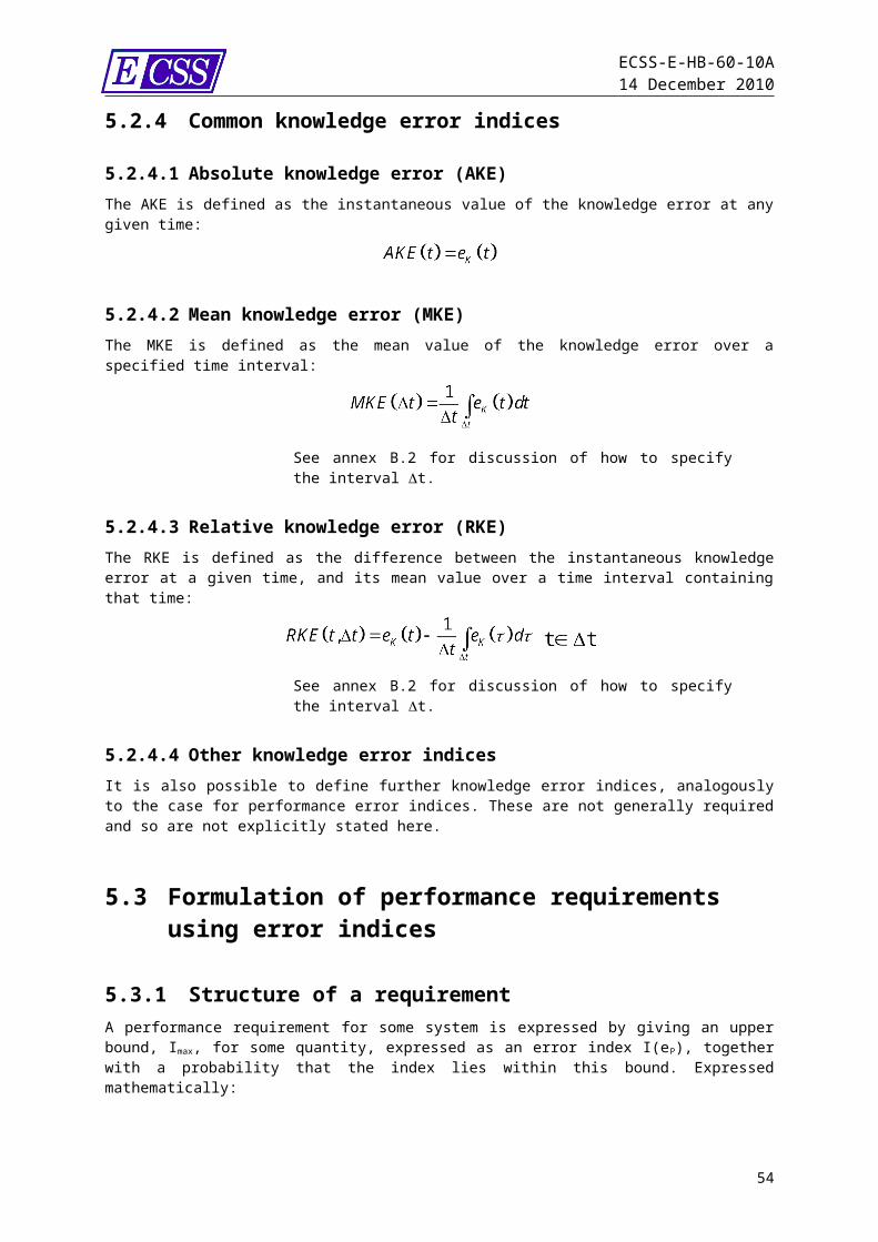
ECSS-E-HB-60-10A14 December 2010
NOTE 2 The estimated standard deviations obtained from these summation formulae are conservative. Alternative summation rules can be found in the literature which use a modified summation rule in order to compensate for potential underestimates of variance. These are not recommended for reasons discussed in annex B.6.3
5.5.5 Comparison with requirementsThe original requirement being assessed by the budget is
Once the total error distribution (i.e. total, total) has been obtained, the following to be done is to compare it to this requirement.ll. Given the assumption that the total distribution has a form close to Gaussian, there
are two ways in which this can be done:
1. If the mean is zero or small ( ), then if the confidence level PC of the requirement is equivalent to the nC level of a Gaussian distribution, the requirement is met if
This is the approach generally used in practice, however it is only valid if the final distribution is close to Gaussian (i.e. the conditions in the previous clause are verified) and if the mean value is small enough to be ignored. 2. If the approximations in 1.1.1.11 are not met (significant mean) then the
budget is compliant with requirements providing that
NOTE 1 E(x) is the error function.NOTE 2 The formula is derived by noting that the requirement is equivalent to
Where P(Itotal) is the PDF of the total error. mm. If the assumption that the final distribution is close to Gaussian is not valid, then
neither of the approximations in 1.1.1.11 and 1.1.1.12 can be used, and P(Itotal) is found by numerical methods. This is the case:1. If there is only a small number of errors contributing to the total (unless the
errors are all near Gaussian)2. If a small number of non-Gaussian errors dominates the budget.
5.5.6 Practical use of a budget (Synthesis)Subclauses 5.5.1 to 5.5.5 (and associated annexes) give the mathematics behind the budgeting process. This clause synthesises the results to provide an overview of how such budgets are compiled in practice.nn. For each index, a table is created listing all sources of errors
54
ECSS-E-HB-60-10A14 December 2010
NOTE If necessary a separate list can be compiled of error sources considered but shown to be negligible
oo. If required, each error source is assigned into one of several classesNOTE Typical classes: biases, harmonic errors, random errors (Gaussian distribution), random errors (uniform distribution), transients. See annex B.5.
pp. The errors within each class are summed as described in jj, and these values are entered in the table
qq. The total errors per class are summed to give the overall error as described in kk, and these values are entered in the table
rr. This overall error is compared to the requirement as described in 5.5.5An example of such a process is given in Table 5-12, for an example where the means of all distributions are negligible. Tables such as this should be created for each error index on which requirements are placed.
55
ECSS-E-HB-60-10A14 December 2010
Table 5-12Example of a table used for a performance budget (APE for Euler angles)
Error name Error class
Standard deviation of error angle about each axisx y z
Bias error 1 B Bx(1) By(1) Bz(1)
Bias error 2 B Bx(2) By(2) Bz(2)
Bias error Nb B Bx(Nb) By(Nb) Bz(Nb)
Harmonic error 1
H Hx(1) Hy(1) Hz(1)
Harmonic error 2
H Hx(2) Hy(2) Hz(2)
Harmonic error Nh
H Hx(Nh) By(Nh) Hz(Nh)
Random error 1
R Rx(1) Ry(1) Rz(1)
Random error 2
R Rx(2) Ry(2) Rz(2)
Random error Nr
R Rx(Nr) Ry(Nr) Rz(Nr)
Total bias error
Total harmonic error
Total random error
Total error
Total error x nC nCTotal,x nCTotal,y nCTotal,z
Requirement at nC max,x max,y max,z
NOTE 1: This example assumes that means are zero, which is not the most general caseNOTE 2: Harmonic errors are assumed not to have similar periods
56
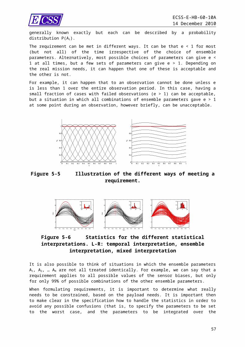
ECSS-E-HB-60-10A14 December 2010
6Intrinsic performance indicators for
closed-loop controlled systems
6.1 OverviewThe definitions and methods developed in Clause 5 (“signal performance error indices and analysis methods”) deal with extrinsic properties of control systems. They can apply on any type of time-dependent output signal whatever the nature of the system. No assumption is made for what concerns the control structure; actually even purely passive plants can be processed according to those techniques.Nevertheless in practice the systems involving closed-loop control represent an important subset for which intrinsic performance indicators are needed as well. For such architectures it is not always sufficient to specify (and to verify) the performance in terms of output signals only; it can be necessary to verify also the internal behaviour of the system.As an example to illustrate this introduction, one of the most common requirements set for such systems concerns the stability margins (such as gain and phase margins for linear SISO feedback loops). This can be considered as a performance requirement, although not directly related to the nature of the output signals. Such margins are very commonly specified by customers to suppliers to ensure that the controlled system is able to operate properly in the presence of uncertainties in the plant model or in the environment.This clause identifies and defines the main features describing the intrinsic behaviour of a closed-loop controlled system, which are commonly subject to specification. It also identifies those to be analysed and verified by the control study team.It is not intended here to extend the scope to the technical domain of control design and analysis (synthesis techniques, advanced analysis methods etc.). This document cannot synthesise nor substitute for the huge literature available in this domain. The purpose here is to review the elements that specify the design, and clearly not to deal with the design process itself.
6.2 Closed-loop controlled systems
6.2.1 General closed-loop structureIn a general closed-loop controlled system, the states of the plant are measured through a set of sensors, from which the controller actively works out the physical feedback commands to be applied to the plant by a set of actuators.
57
ECSS-E-HB-60-10A14 December 2010
The objective of the closed loop is to compensate for the disturbance that affects the system. The nature and the design of the controller is driven by the nature of the disturbance and by the desired performance (for instance, an integral type drives the effect of a constant disturbance to zero). This objective is a key driver of the control design, which is excluded from the scope of the present document.The controller can be implemented either in analogue, or in digital, or both.The simplified schema for a closed-loop controlled system is described on Figure 6-7 hereafter, in accordance with the more general, higher level structure of Figure 4-1 and Figure 4-2. The schema includes a plant (or a dynamics, D) and a controller K. The aim is to follow a control reference, the control feedback being worked out based on the difference between the sensors outputs and the objective. The system is disturbed by external disturbances (such as a perturbing torque for example) and by a measurement noise.
Plant (dynamics)
DKControl
Controlreference
Disturbance
Controlperformance
Measurementnoise
Feedback loop
d
vy
m
ym
r
++
++
–+u
Plant (dynamics)
DKControl
Controlreference
Disturbance
Controlperformance
Measurementnoise
Feedback loop
d
vy
m
ym
r
++
++
–+u
Figure 6-7Simplified scheme for a closed-loop controlled system
6.2.2 General definitions for closed-loop controlled systems
6.2.2.1 GeneralThis clause 6.2.2 presents some basic prerequisite definitions for general concepts in relation to closed-loop controlled systems. The reader should refer also to Annex A for more details, if required.
6.2.2.2 Definitions
6.2.2.2.1 linear time invariant system (LTI)important class of closed-loop systems whose behaviour can be fully described by a set of linear, time invariant differential (continuous) or recursive (discrete) equations
NOTE Such ideal systems do not exist in the real world. Nevertheless in many cases the behaviour of a real system around an equilibrium position can be locally approximated by a LTI representation (linearised model). The very large mathematical background of linear algebra can then be used to analyse any LTI system in an
58
ECSS-E-HB-60-10A14 December 2010
extensive and systematic way. This is why such representations are of major practical importance.
6.2.2.2.2 single input, single output system (SISO)
system with an input vector and an output vector of dimension 1.NOTE A SISO LTI system can be formally described by a scalar transfer function where
is the Laplace’s variable
6.2.2.2.3 multiple input, multiple output system (MIMO)
system with an input vector or an output vector (or both) of dimension > 1.NOTE A MIMO LTI system can be formally described by a matrix transfer function where
is the Laplace’s variable
6.2.2.2.4 feedback
process whereby some proportion of the output signal of a system is passed (fed back) to the input.
NOTE This is often used to control the dynamic behaviour of the system.
6.2.2.2.5 closed-loop transfer functiondescribes the input/output behaviour of a controlled system when the return signal is fed back into the controller.
6.2.2.2.6 open-loop transfer function
describes the input/output behaviour of a controlled system when the return signal is not fed back into the controller.
NOTE The open-loop transfer function is used typically for purposes of analysis of the closed-loop properties (in particular its stability margins).
6.2.2.2.7 state space representation
mathematical model of a physical system as a set of input, output and state variables related by first-order continuous or discrete differential equations.
NOTE To abstract from the number of inputs, outputs and states, the variables are expressed as vectors and the differential and algebraic equations are written in matrix form. The state space representation (also known as the "time-domain approach") provides a convenient and compact way to model and analyze systems with multiple inputs and outputs.
6.2.2.2.8 Nichols plot
graph in which the logarithm of the magnitude is plotted against the phase of a frequency response on orthogonal axes.
NOTE This plot combines the two types of Bode plot — magnitude and phase — on a single graph, with frequency as a parameter along the curve.
59
ECSS-E-HB-60-10A14 December 2010
6.3 Stability of a closed-loop controlled systemIn the current context of closed-loop controlled systems and automatic control engineering, the “stability” is the intrinsic property defined as the ability of a system to remain indefinitely in a bounded domain around an equilibrium position or around an equilibrium trajectory when submitted to small external disturbances.It is not possible to be more specific while dealing with general systems. Several types of stability are defined in the specialised literature according to the nature of the system (such ad bounded input, bounded output stability, Lyapunov stability for example).For LTI systems it is possible to go further and to give a clear characterisation of the stability, which can be seen as a definition, based on the properties of their state space representations:
A continuous LTI system is stable if and only if all of the eigenvalues of its state matrix have strictly negative real parts.A discrete LTI system is stable if and only if all of the eigenvalues of its state matrix have modulus strictly smaller than 1.
It should be noted that this definition ensures not only that the elements of the output vector are bounded, but also that all of the components of the (internal) state vector are bounded. This is a strong stability definition.
NOTE 1 This document does not the different methods available to verify the stability. The general rule is clearly formulated, based on the eigenvalues of the state matrix. The general approach is based on a numerical computation of these eigenvalues. In some situations alternative methods can be used: graphic (Nyquist locus), analytic (Routh-Hurwitz criterion for example); see specialised textbooks for more details.NOTE 2 This discussion about stability can apply to any time of system, not necessarily involving control feedback (for example, passive natural dynamics about an equilibrium state). Nevertheless this document mainly focuses on actively controlled systems.
6.4 Stability margins
6.4.1.1 OverviewConsidering the stability properties are verified according to the definition given in 6.3 for LTI systems, it becomes of interest to quantify the degree of stability of a system. From a very general point of view, this degree of stability can be defined as the amplitude of uncertainties on the physical parameters describing the control system (plant, sensors, actuators, controller) for which the closed loop remains stable.Again it is not possible to be more specific in the general case. But further consideration can be developed assuming we are dealing with LTI systems.
60
ECSS-E-HB-60-10A14 December 2010
6.4.2 Stability margins for SISO LTI systems
6.4.2.1 GeneralThis clause 6.4.2 defines the quantified stability margin indicators for SISO LTI systems.
6.4.2.2 Definitions
6.4.2.2.1 gain marginamount of gain increase required to make the open-loop gain unity at the frequency where the phase angle is -180°
6.4.2.2.2 phase margin
difference between the phase of the open-loop transfer function and -180° (modulo 360°) when the gain is unity
NOTE 1 The gain margin is expressed in dB. To avoid any ambiguity, it is important to clearly state the convention used to define the dB scale.NOTE 2 The phase margin is expressed in degrees.NOTE 3 In some cases there can exist several values for the gain and phase margins. For example most systems controlled by a PID exhibit two gain margins: one low frequency margin, and one high frequency margin.
6.4.2.2.3 modulus marginminimum distance from the critical point -1 to the open-loop transfer function
NOTE 1 The modulus margin is expressed in dB. To avoid any ambiguity, it is important to clearly state the convention used to define the dB scale.NOTE 2 This margin is an extension of the gain and phase margins to a more general type of loop uncertainty.NOTE 3 Unlike gain and phase margins there is one and one only modulus margin whatever the system.
6.4.2.2.4 delay margin
maximum value of a pure delay in the loop such that the closed-loop system remains stable
NOTE 1 The delay margin is expressed in seconds.NOTE 2 According to the definition here there is one and one only delay margin.NOTE 3 This delay margin can extend to MIMO control laws assuming that the delay is identical for all the channels.
6.4.2.3 DiscussionThese stability margins are calculated from the properties of the open-loop transfer function according to the formulas gathered in Table 6-13.
NOTE 1 It is meaningless to establish any stability margins before proving that the closed-loop system is stable. The properties of the Nichols plot of the open loop transfer function are not sufficient to prove the stability of
61
ECSS-E-HB-60-10A14 December 2010
the closed loop in the general case. Demonstrating stability can be done analysing the eigenvalues of the state matrix as presented in clause 6.3.NOTE 2 In practice the stability margins are determined graphically from the position of the open-loop transfer function with respect to the critical point -1 (see any academic automatic control handbook for details). This can be done either using root locus, Bode, Nichols or Nyquist representations.NOTE 3 Classically the stability requirements for SISO LTI systems are formulated in terms of gain and phase margins. Modulus and delay margins specifications are far less common. This is a fact, but this does not mean that they are less pertinent a priori.NOTE 4 Classically again, the specified values for stability margins are very often 6 dB for the gain, and 30° for the phase. These values are in part related to historical reasons (see clause 6.4.4); they are orientative.
Table 6-13Formulas for the usual SISO stability marginsGain margin
being the angular frequency(ies) where the phase of the open-loop transfer function equals -180° (modulo 360).
Phase margin
being the angular frequency(ies) where the modulus of the open-loop transfer function equals 0 dB.
Modulus margin
Delay margin
angular frequency(ies) where the modulus of the open-loop transfer function equals 0 dB (0 dB open-loop cut-off frequency).
An example of stability margins assessment for a continuous SISO system is given on Figure 6-8 hereafter using the Nichols locus. For information, this example corresponds to a single-axis attitude dynamics with one flexible mode, controlled by a first order phase-lead plus an elliptic low-pass filter:
62
ECSS-E-HB-60-10A14 December 2010
Figure 6-8Example of gain and phase margins identification
The proof of the closed-loop system stability was first given by computing the eigenvalues of the state matrix (all real parts are strictly negative). On Figure 6-8, (1) corresponds to the gain margin (17 dB), (2) corresponds to the phase margin (28 deg); the modulus margin is 6.3 dB for this example, which means that the smallest modulus of complex feedback uncertainty that can drive the system unstable is 0.484.
6.4.3 Stability margins for MIMO LTI system – S and T criteria
6.4.3.1 GeneralThe stability margins defined for SISO LTI systems do not apply to MIMO case (except under some conditions the delay margin). The specific stability indicators to be used when dealing with such systems are based on the so-called sensitivity and complementary sensitivity functions, defined in clause 6.4.3.2.
6.4.3.2 Definitions
6.4.3.2.1 output sensitivity function
closed-loop transfer function between the control reference r and the feedback error term
6.4.3.2.2 input sensitivity function
closed-loop transfer function between the external disturbance d and the total action v
63
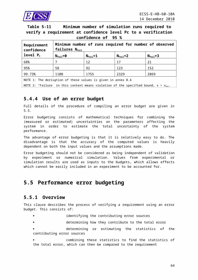
ECSS-E-HB-60-10A14 December 2010
6.4.3.2.3 output complementary sensitivity function
closed-loop transfer function between the control reference r and the control performance y
6.4.3.2.4 input complementary sensitivity function
closed-loop transfer function between the external disturbance d and the control command u
NOTE 1 With the control loop structure and notations introduced by Figure 6-7, these functions are:
, ,
,
NOTE 2 These sensitivity functions also make sense for SISO LTI systems. In this case, the blocks and commute, so and .
6.4.3.3 DiscussionFor MIMO systems the stability margins are characterised by the norm of the sensitivity and complementary sensitivity functions, which are complex matrix functions of the frequency. The appropriate definition of the norm for these objects is based on the singular values. For a complex matrix , the maximum singular value is given by
The stability margins are determined by the maxima of these singular values over the frequency domain:
The larger these values, the smaller the stability margins. As a consequence specifying a given level of stability margins can be achieved by specifying a maximum value for the singular values above.
NOTE 1 Prior to establishing any MIMO stability margins the closed-loop system has first to be proven stable. The properties of the singular values of the sensitivity functions are not sufficient to prove the stability of the closed loop. Demonstrating stability can be done analysing the eigenvalues of the state matrix as presented in clause 6.3.NOTE 2 Classically, the specified value for the maximum singular value is very often 2 (6 dB):
6 dB
6 dB
6 dB
6 dB
64
ECSS-E-HB-60-10A14 December 2010
Please note that this rule is merely indicative (see clauses 6.4.4 on).NOTE 3 These margin criteria on singular values are the only available for MIMO systems, but they also can be used for SISO systems. In this case they represent a valuable alternative to the classical gain and phase margins specification. Keeping the singular values below 6 dB ensures (approximately) a gain margin of 6 dB and a phase margin of 6 dB.NOTE 2 More specifically for a SISO system, there is an equivalence between the modulus margin and the singular value of the complementary sensitivity functions (see annex A).
6.4.4 Why specifying stability margins?The usual way of specifying stability margins (for SISO LTI systems) is based on gain and phase margins. This approach is partly due to the fact that the first generation control loops were implemented using analogue devices, prone by nature to uncontrollable gain and phase shifts (thermal, ageing effects on hardware components). The margins were then required to ensure that the system remains stable, should the physical controller be affected by such variations.Now in space domain most of the controllers are implemented numerically (although some rare exceptions still remain). There are no longer such physical uncertainty about the behaviour of the controller itself; it can then be anticipated that the margins requirement should be loosened – more or less – to account for this improvement. However in practice this is not the case. The main reason is that whereas uncertainties reduced at controller’s level, they tended to increase at plant’s level. Taking the example of AOCS control loops, the dynamics of the satellites have grown in complexity over the past years, due to large flexible appendages, large sloshing fuel masses for example; in addition pointing requirements also tend to become more and more stringent. The stability margins are intended to cope with the growing uncertainties related to these elements. Note also that in some situations the same controller can be used during different phases of the mission for which the spacecraft characteristics can present significant variations (BOL/MOL/EOL mass and inertia evolution for example). In such cases the controller needs to operate properly over a certain range of plant behaviours.In addition to those basic technical considerations, it happens that (for efficiency purposes) satellite manufacturers sometimes aim at designing and tuning controllers not for one single satellite, but for a range of satellites featuring homogeneous – but not strictly equivalent – characteristics. Another aspect of the stability margins is related to the overshoot of the closed loop in frequency domain. The modulus margin directly gives the frequency peak magnitude; the “usual” combination 6 dB gain margin and 30 deg phase margins ensures in general that the closed loop overshoot also remains below 6 dB; so does the singular values criterion of 6 dB for MIMO systems. From the point of view of the control engineer, these values can also be seen as “design goals” to get a satisfactory behaviour of the closed loop.Putting things together, it can be seen that specifying stability margins also involves considerations on robustness and performance. In any case, it makes sense that any stability margin specification is associated to an uncertainty domain over which it is intended to be verified.
65
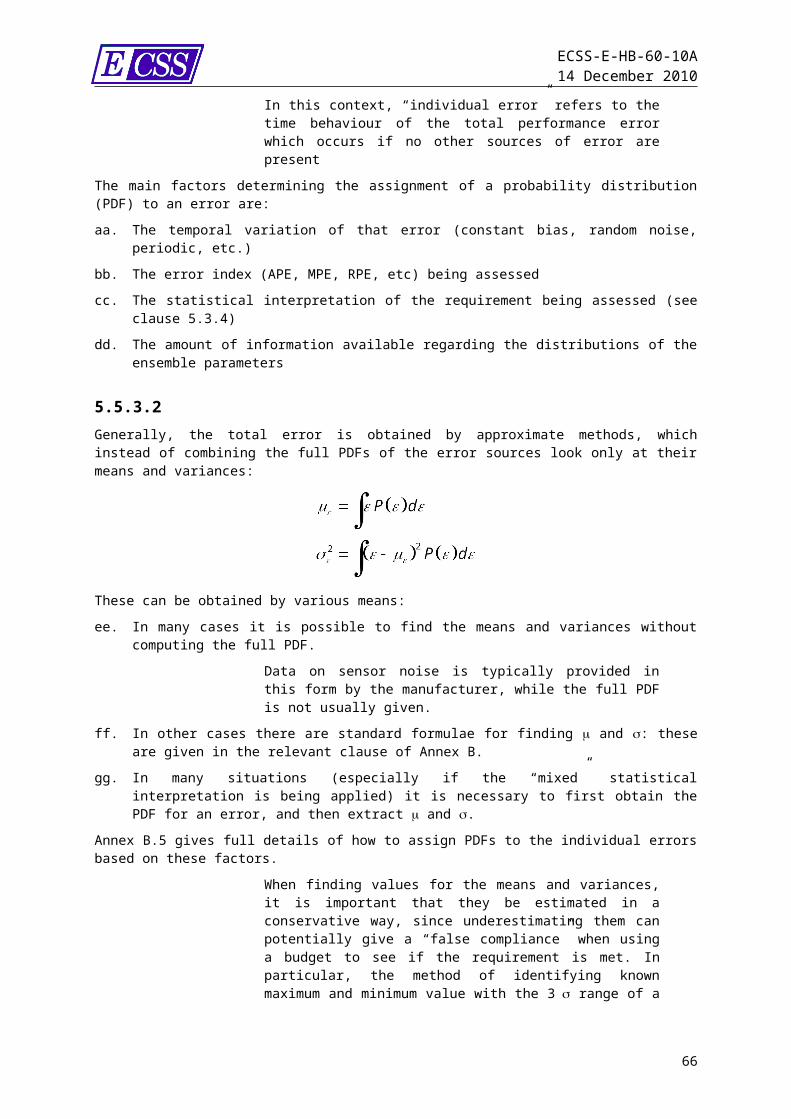
ECSS-E-HB-60-10A14 December 2010
6.5 Level of robustness of a closed-loop controlled system
A general definition to robustness is provided in ECSS-E-HB-60A, 3.2.30 as the property of a control system to achieve the control objectives in spite of uncertainties. Stated slightly differently the level of robustness of a control system is therefore characterised by the size of the uncertainty domain over which the control objectives are achieved. “Achieved” can be understood in two senses:
Strong sense: size of the domain of signal and model uncertainties for the system and its environment for which the specified performance level is met. Weak sense: size of the domain of signal and model uncertainties for the system and its environment for which the system still operates but with degraded performances.
There is a close link between stability margins and robustness, although both concepts are not fully equivalent.
6.6 Time & Frequency domain behaviour of a closed-loop controlled system
6.6.1 OverviewThis clause lists and defines some additional time and frequency domain performance indicators for closed-loop controlled systems that can be subject to specification.
6.6.2 Time domain indicators (transient)
6.6.2.1 GeneralConsider a stable controlled system perfectly converged around an equilibrium position. Let a step be applied to the value of the control objective. The transient response of the closed-loop system can be described in terms of overshoot, response time and settling time.
6.6.2.2 Definitions
6.6.2.2.1 overshoot (transient)maximum factor by which the transient response exceeds the control reference, should this occur.
NOTE 1 If the response never exceeds the objective no overshoot is defined.NOTE 2 The wording “overshoot” also applies to frequency domain properties of transfer functions (response magnification at resonance frequencies).
6.6.2.2.2 response timethe response time is defined by the date at which the system response first crosses the control reference
66
ECSS-E-HB-60-10A14 December 2010
NOTE Again if the response never crosses the reference no such response time is defined; instead the “settling time” defined hereafter can be used.
6.6.2.2.3 settling timetime after which the system response remains indefinitely within a (small) predefined interval around the value of the control reference
6.6.2.3 DiscussionThe list of time domain indicators defined in clause 6.6.2.2.1 is not and cannot be exhaustive; several additional time domain indicators can be defined (such as logarithmic decrement, damping factor for example), but they are of lesser practical interest and redundant with the ones in 6.6.2.2.1.An illustration is provided on Figure 6-9 hereafter for the overshoot, the response time and the settling time on a typical transient response.On Figure 6-9, (1) corresponds to the overshoot (1.55, or 3.7 dB), (2) corresponds to the response time (198 s), and (3) corresponds to the settling time at 97% (1350 s).
Figure 6-9 Illustration of the transient response indicators
67
ECSS-E-HB-60-10A14 December 2010
6.6.3 Frequency domain performance indicators
6.6.3.1 GeneralThere also exist several frequency domain performance indicators which can be specified for closed-loop controlled systems.
6.6.3.2 Definitions
6.6.3.2.1 bandwidth
the bandwidth of a controller is defined from a very general point of view as the frequency interval (or intervals) for which the closed-loop behaviour is significantly modified with respect to the natural, uncontrolled dynamics of the system
6.6.3.2.2 cut-off frequency
the cut-off frequency (or frequencies) corresponds to the extrema values of this interval (or these intervals).
NOTE From there comes a common practical definition for the bandwidth, namely the “0 dB open-loop bandwidth” which corresponds to the frequency domain for which the norm of the open loop is greater or equal to 1.
6.6.3.2.3 disturbance rejectionability of the closed-loop control to reduce the effects of the external disturbances on the response of the system, with respect to what it would have been in free dynamics.
NOTE 1 The disturbance rejection performance is fully determined by the modulus of the transfer function
.NOTE 2 Indeed the rejection profile is linked to the bandwidth.
6.6.3.2.4 tracking performance
ability of the closed-loop controlled system to follow the control objective profile along time.
NOTE 1 The tracking performance is determined by the modulus of the transfer function between the control objective and the control error , .NOTE 2 The tracking performance and the disturbance rejection are determined by the same transfer functions. Both are directly related to the bandwidth, those three indicators all characterising the “efficiency” of the controller.
6.6.3.2.5 static gain
modulus of the transfer function of the controller when the frequency tends to zero. NOTE 1 This value does not always exist (for example if the controller includes an integral term, the modulus tends to infinity as the frequency tends to zero).NOTE 2 The value of the static gain is an element of performance for the closed loop. The system response
68
ECSS-E-HB-60-10A14 December 2010
when submitted to a static disturbance is directly given as the ratio (disturbance)/(static gain).
6.6.3.2.6 open loop rejection of natural resonances
maximum level of the peak responses on natural resonances (flexible structural modes for example) as seen on the open-loop transfer function.
NOTE A requirement (if any) of open-loop rejection of natural resonances is closely related to the stability margins, by limiting the possible control/structure interactions.
6.6.3.3 DiscussionThis list of frequency indicators is not exhaustive; several additional indicators can be defined (such as damping ratio, ripple in the band for example), but they are of lesser practical interest and redundant with the ones in 6.6.3.2.An illustration is provided on Figure 6-10 for the bandwidth, the cut-off frequency and the open loop rejection of natural resonances on the Bode plot for a typical controlled system (flexible dynamics, phase-lead control with low-pass elliptic filter).The first plot represents the open loop gain, the second plots overlays the responses of the uncontrolled dynamics and of the closed-loop controlled system.
69
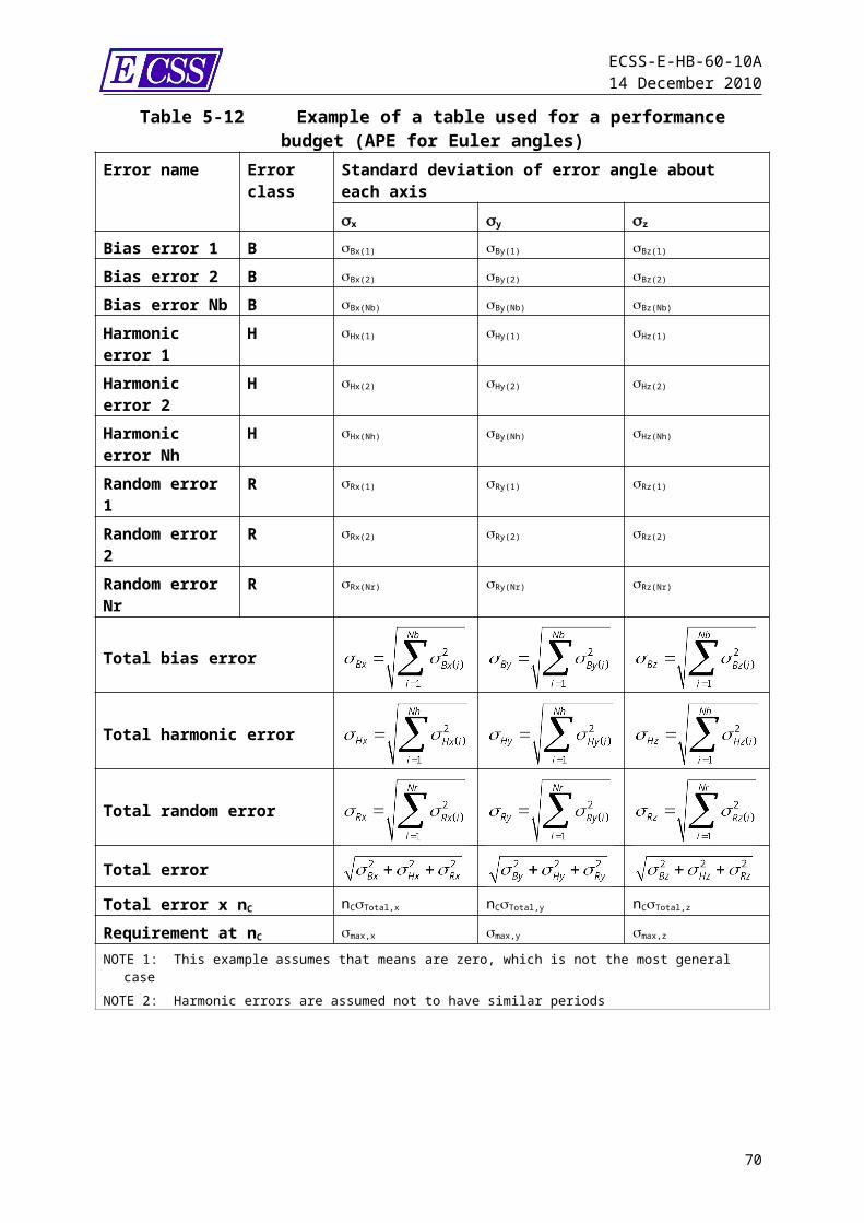
ECSS-E-HB-60-10A14 December 2010
Figure 6-10 Bandwidth, cut-off frequency and rejection of resonances
70
ECSS-E-HB-60-10A14 December 2010
6.7 Formulation of performance requirements for closed-loop controlled systems
6.7.1 GeneralTo keep the presentation as clear as possible, this clause 6.7 and the associated examples mainly deal with the requirements related to stability margins, which are the most frequent in practice, and the most complex to handle. Nevertheless the material developed hereafter also applies to the other intrinsic performance elements, as defined in clause 6.6.
6.7.2 Structure of a requirement The issue of formulating requirements was addressed in clause 5.3 for extrinsic performances. Basically a similar approach can apply to intrinsic requirements. The mathematical statement of the requirement should look as follows, for example for a gain margin:
with the following elements:ss. The exact definition of the property to be constrained (gain margin in our
example).tt. A maximum or minimum allowed value for this index.
uu. The required probability, , that the index is inside the allowed range.
vv. The conditions under which the probability is to apply.By definition, intrinsic properties of LTI systems are time independent; the only statistical dimension of the problem (point d. of the list above) consists of the uncertainties of the system parameters themselves. A pure ensemble interpretation of the requirement can be assumed. To complete the formulation of the requirement, it is therefore necessary and sufficient to define the uncertainty domain for the physical parameters describing the system.To date this type of probability-based formulation is extremely infrequent in the frame of space project. The most common type of requirement is stated as:
“The gain margin shall be better than 6 dB.”This is extremely ambiguous. How should it be interpreted by the control designers:
“verify that the gain margin is better than 6 dB for the nominal parameters of the control system” (unformulated implication: the 6 dB margin aims at covering the uncertainties on the parameters values), or “verify that the gain margin is always better than 6 dB, even with dispersed parameters values” (unformulated implication: the closed-loop behaviour is “equally good” even for extreme dispersion cases)?
These two interpretations are very different and lead to very different design options (with complexity and cost consequences). But both are pertinent, and make sense in practice, according to the nature of the project and of the high level mission needs. As a minimum, it is important to raise the ambiguity by formulating the actual need, choosing between the two interpretations above.
NOTE There is a obvious connection with the concept of “robustness” introduced in clause 6.5. Clearly the statement of the second bullet here above induces a
71
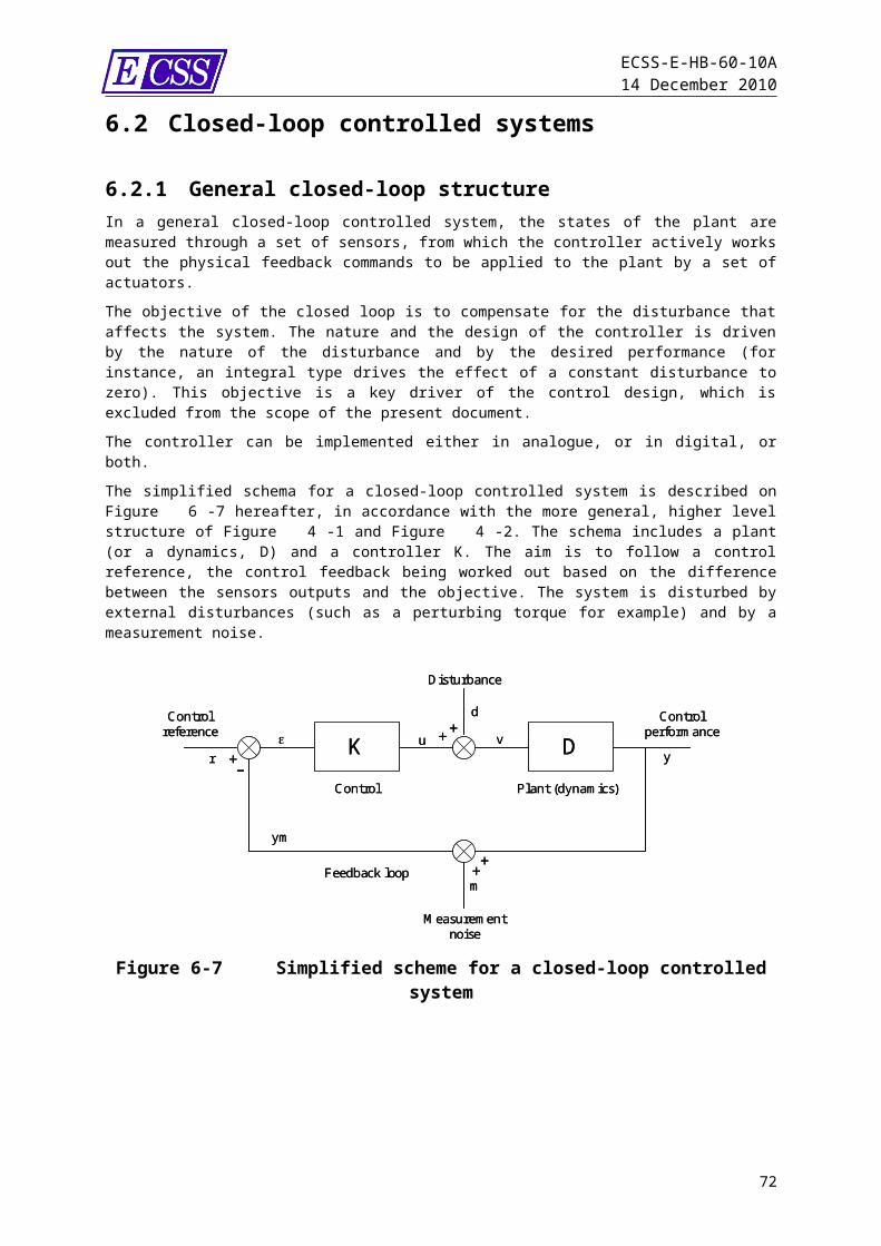
ECSS-E-HB-60-10A14 December 2010
strong requirement in terms of robustness to uncertainties, whereas the first does not (or significantly less).
Propositions for raising the ambiguity in practice can be found in clause 6.7.4.
6.7.3 Specification for general systems (possibly MIMO, coupled or nested loops)
For general systems (not necessarily SISO) this notion of uncertainty domain over which the margin specification applies, is still pertinent. The problem in terms of stability margins is that the simple, scalar (or complex) margins (gain, phase, delay, module) defined for mono-dimensional loops cannot easily be generalised to MIMO loops, coupled or nested systems.Indeed the definition of the margins maps the nature and the structure of the uncertainties that affect the control system. For a mono-dimensional loop this is easy to figure out; but for more complex systems there can be several places where uncertainties appear, possibly in a non-commutative way, that also can combine in a non-intuitive manner (see annex A, clause A.3.1.2). A possible solution to specify stability margins is to require the sensitivity and complementary sensitivity functions to be kept below a given maximum value (6 dB for example), these functions being defined on the appropriate loop checkpoints covering the different types of uncertainties that affect the control system.
6.7.4 Example of stability margins requirementBased on the two previous clauses, this is an example of formulation for stability and stability margins requirement, which can apply to a very general control system, as well as to an elementary, SISO loop.Note how this formulation avoids the risk of ambiguity mentioned in clause 6.7.2 by clearly stating the uncertainty domain(s) over which the margins are asked to be verified. Here a “reduced” uncertainty domain is defined, where a nominal level of stability margins is specified; in the rest of the uncertainty domain, degraded margins are accepted:ww. Stability properties:
“The stability properties shall be unambiguously demonstrated over the whole uncertainty domain” (For example, by examining the eigenvalues of the closed loop state matrix).
xx. Loop checkpoints:“The loop checkpoints shall be identified according to the nature and the structure of the uncertainties that affect the system”; These loop checkpoints correspond to the points where margin requirements need to be verified.
yy. For MIMO systems, the nominal margins correspond to a peak value of the sensitivity and complementary sensitivity functions kept below TBD dB (usually 6 dB). For SISO systems the nominal margins are either defined in terms of gain and phase (usually 6 dB, 30 deg.) or in terms of modulus margins (usually 6 dB). “The nominal stability margins shall be demonstrated for all of the loop checkpoints over the reduced uncertainty domain” (1 uncertainty domain for example);
zz. (facultative) The degraded margins correspond to a peak value of the sensitivity and complementary sensitivity functions kept below TBD dB (3 dB for example). For SISO systems the degraded margins are either defined in terms of gain and
72
ECSS-E-HB-60-10A14 December 2010
phase (3 dB, 15 deg. for example) or in terms of modulus margins (3 dB for example). “The degraded stability margins shall be demonstrated for all of the loop checkpoints over the rest of the uncertainty domain” (3 uncertainty domain for example)
NOTE 1 The figures given here are “usual” ones; But this does not mean they correspond to an absolute rule.NOTE 2 For these formulations, the probability level defined in clause 6.7.2 is taken equal to 1 (which is equivalent to a requirement on the extremum value).NOTE 3 A conservative approach consists on verifying nominal stability margins for the whole uncertainty domain (or 3 uncertainty domain for example). NOTE 4 The approach to be selected depends on the nature of the project, on the mission profile etc. There is no general rule. NOTE 5 In the case of a common design and tuning for a range of satellites, clearly nominal stability margins are supposed to be verified all over the parameters defining the range in order to get an homogeneous behaviour whatever the satellite.NOTE 6 In the case of an elementary SISO system there is one single loop checkpoint. The requirement is equivalent to a gain, phase or modulus margin (over a given uncertainty domain).NOTE 7 As a facultative option a requirement in terms of delay margin can be added to the one on the sensitivity functions (if this makes sense in the context of the project).
6.8 Assessing compliance with performance requirements
6.8.1 Guidelines for stability and stability margins verification The complete sequence for stability and stability margins verification for a real system can be split into:
linearization of the system (when possible) in the neighbourhood of its operational conditions, design and tuning of the controller with respect to the linearized system (not in the scope of this document), verification of the system stability properties (stability, margins, robustness, advanced methods) using the linear analysis techniques described in the previous clauses, taking into account the parametric uncertainties of the system (see next clause) final validation by performing time simulations with the complete system (including non-linear features), analysing the response signal behaviour.
NOTE There exists analysis techniques dealing with stability properties of non linear systems, mostly applicable to simple cases. Ultimately it is possible that
73
ECSS-E-HB-60-10A14 December 2010
investigation of these systems cannot be done by others than by numerical simulation.
6.8.2 Methods for (systematic) robustness assessmentIn practice it can be difficult to ensure that this verification is fully exhaustive, due to the number of uncertain parameters and to the size of the domain that should be investigated. Scanning the full domain by a series of discrete sets of numerical values can lead to huge simulation times. Consider for illustration a simple (simplified) satellite dynamical model with a rigid central body and two steerable solar arrays with three flexible modes each: the elementary parameters required to describe this dynamics are
the rigid inertia matrix of the full satellite (6 parameters), the cantilever frequencies for the flexible modes (6 parameters), the cantilever damping ratios (6 parameters), the modal coupling factors of the flexible modes (36 parameters, reducing to 12 considering pure modal shapes), and the two steering angles.
Even considering a fixed, worst case damping ratio and pure modal shapes the sensitivity analysis should run over 26 elementary parameters, which makes it hardly manageable in practice. The search for a worst case of stability margins is partly driven by engineering feeling (for simple configurations and control laws, the smaller the inertia, the higher the coupling factor, the smaller the cantilever frequency often lead to minimum margins).Systematic techniques exist based on advanced methods (for instance based on “M-decomposition” of the uncertain system), which allow – with some limitations – for a direct identification of the worst combination of uncertainties leading to the loss of the stability properties. Nevertheless these techniques are difficult to generalise and can reach their limits for systems with a large number of uncertain parameters; they cannot be set as a standard approach for stability verification.Investigating the whole uncertainty domain for stability analysis is therefore similar to developing a Monte-Carlo simulation plan for performance assessment, including the need of using the same statistical rules.
74
ECSS-E-HB-60-10A14 December 2010
7Hierarchy of control performance
requirements
7.1 OverviewClauses 5 and 6 of this document have developed a large (and open) set of performance indicators, of methods and guidelines for formulating a requirement and for verifying these requirements in the frame of a space project. Now the question is: how to use these elements to work out a consistent set of requirements? More specifically:
Performance properties to be systematically specified. Other properties and parameters to be specified. Properties and parameters not to be specified.
The intention of this clause is not to address the question of building a requirement from a general point of view; this is definitely out of the scope of this document. But in the current context it is worthwhile introducing some guidelines of good sense in the domain of control engineering.
7.2 From top level requirements down to design rules
7.2.1 GeneralScanning the list of extrinsic and intrinsic performance indicators listed in clauses 5 and 6, it can be seen they correspond to distinct levels of requirements:
7.2.2 Top level requirementsThe top level requirements are the formulation of the end user needs in terms of control performances. Taking the example of an AOCS for an Earth observation mission, top level requirements are expressed in terms of APE, RPM, AKE, which contribute respectively to the image location, to the image quality and to the image localisation.Clearly providing these requirements is mandatory in all cases; they constitute a key design driver. Refer to clause 5 for guidelines and recommendations on how to properly formulate the appropriate requirements.
75
ECSS-E-HB-60-10A14 December 2010
7.2.3 Intermediate level requirementsAn intermediate level set of requirements corresponds to performance elements that are more or less invisible for the end user but which actively contribute to the end-to-end system performance.Stability margins are a typical example for this class of performance indices. Nominally, a spacecraft user never “sees” these margins by inspecting the on-orbit behaviour. These margins are just provided by design so that the control system behaves properly. Basically these indicators are used by control engineers to optimise the controller design, and pre-validate its behaviour before going to more detailed simulation campaigns (including non linear effects). Going to the extremes, such requirements can then be seen as unnecessary and superfluous. Going back to the discussion of clauses 6.4 and 6.5, if the higher level requirement is stated (for example) as:
“All pointing and knowledge specifications (APE, RPE, AKE etc.) shall be met over the 3 domain of uncertain parameters”,
Then it is crucial that good stability margins are ensured a fortiori. On the other hand, the risk of not putting a requirement on these margins is that the actual design margins are not exhaustively proved by the end-to-end simulation campaigns (by definition Monte-Carlo simulations are never exhaustive seen the number of uncertain parameters that affect the system).This is why although not strictly mandatory, such intermediate level requirements are still pertinent in practice to drive the design trade-off – provided they are formulated without ambiguity and in accordance with the physics they convey, as discussed all along clause 6.7. In most cases these requirements are useful for the user and for the designer to get confidence in the proper behaviour of the control system.
NOTE Specifying too stringent stability margins can be counterproductive when considering the trade-off between stability and performance.
7.2.4 Lower level requirements – Design rulesAt the bottom of the requirement hierarchy, some performance indices can be identify that characterise the innermost behaviour of the control system, without direct intuitive relationship with the end-to-end performance as expected by the end user.Bandwidth, cut-off frequency, static gain etc. are good examples of such low level performance indices. Except in very specific situations (for example, to prevent interference between two control loops operating on a given system, it can be pertinent to specify some kind of minimum bandwidth separation), these elements should not be specified. Tuning an appropriate static gain, or sizing an adapted bandwidth is a design action, which should be based on design rules and not on specifications. Past experience shows that putting inappropriate requirements on such low level design indicators can have counterproductive consequences (see also clause 7.3).
7.3 The risks of counterproductive requirements
7.3.1 An example of counterproductive requirementTo illustrate the risks of counterproductive requirements, let us consider the example of a requirement put on the design of a spacecraft AOCS of the form:
“All natural resonances shall be rejected by at least 6 dB (open loop)”.
76
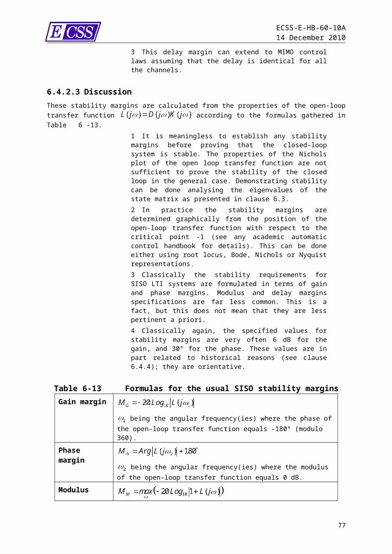
ECSS-E-HB-60-10A14 December 2010
It can be found reasonable at first sight to provide by design such a rejection so as to limit the potential coupling between the control loop and the flexible modes subject to some uncertainties.A first remark however is that putting such a requirement can be superfluous provided stability margins have already been specified. Verifying stability margins with a representative flexible dynamics ensures that there is no risk of destabilisation of the control loop by the flexible modes.In addition a harmful by-product of this requirement is to ban from the design trade-off a class of control techniques based on “phase stabilisation” of the flexible modes, which can be optimal in terms of performances under some conditions, since less constraining in terms of static gain tuning (this is for example the control strategy used in the frame of the whole SPOT satellites family). In the general case the requirement above is not only superfluous but also counterproductive.
7.3.2 How to avoid counterproductive control performance requirements?
In the specific domain of control engineering avoiding the risk of counterproductive requirements is not always easy because the techniques are constantly improving in this domain, and some requirements that used to make sense twenty or even ten years ago can prove obsolete today – see for example the discussion on the “traditional” 6 dB/30° gain and phase margins (clause 6.4.4).As a general recommendation attention should be paid to put requirements at the right level by focussing on the real end-to-end needs, and to avoid lower level requirements which are already covered (implicitly) by higher level ones.In practice the lower-level elements listed in clause 7.2.4 should not be subject to formal specification, except if justified by very specific needs.
77
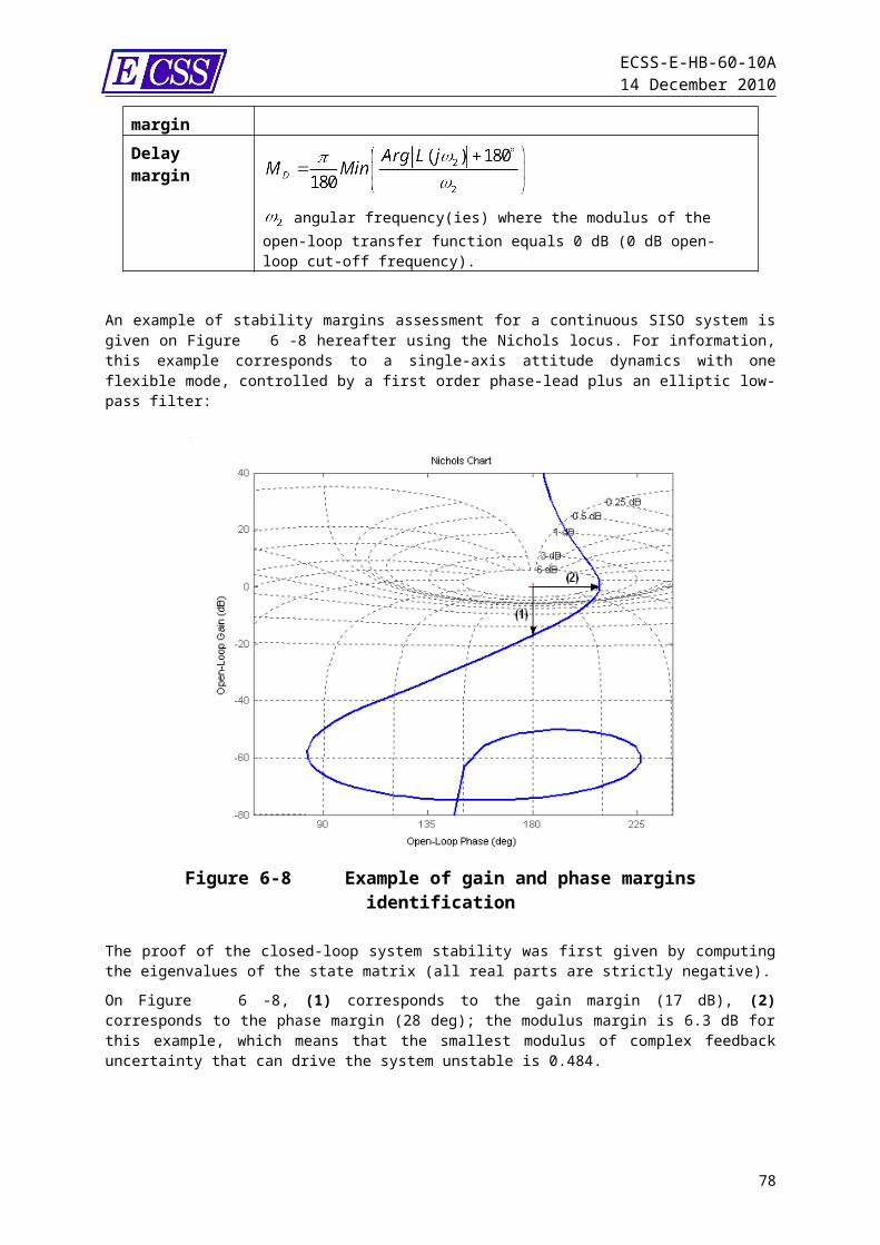
ECSS-E-HB-60-10A14 December 2010
Annex ALTI systems
A.1 OverviewThis informative annex reminds some high level properties of LTI systems, in support to clause 6 of this document. It is not meant to substitute to more complete and focused textbooks dealing with automatic control design, a large number of which can be found in the specialised literature. The scope here is to gather the minimal set of basic elements required to substantiate and to illustrate the relevant developments in the document’s main body.
A.2 General properties of LTI systems
A.2.1 Simplified structure of a closed-loop controlled systemFigure A-1 shows the simplified structure of a closed loop controlled system, featuring a plant (dynamics) D and a controller K, with a control reference r, submitted to external disturbances d and to a measurement noise m:
Plant (dynamics)
DKControl
Controlreference
Disturbance
Controlperformance
Measurementnoise
Feedback loop
d
vy
m
ym
r
++
++
–+u
Plant (dynamics)
DKControl
Controlreference
Disturbance
Controlperformance
Measurementnoise
Feedback loop
d
vy
m
ym
r
++
++
–+u
Figure A-1: Simplified scheme for a closed-loop controlled system
78
ECSS-E-HB-60-10A14 December 2010
A.2.2 Representation of LTI systems
A.2.2.1 State space representation (time domain)
A.2.2.1.1 Continuous LTI system
The general state space representation for a continuous LTI system is as follows:
where is the (time dependent) input vector, is the output vector, is the (internal) state vector,
are four real, constant matrices.
NOTE The square matrix is generally named the “state matrix”.
A.2.2.1.2 Discrete LTI system
The general state space representation for a discrete LTI system is as follows:
where is the input vector at time ,
is the output vector at time ,
is the (internal) state vector at time ,
are four real, constant matrices.
NOTE The square matrix is generally named the “state matrix”.
A.2.2.2 Transfer function representation (frequency domain)
A.2.2.2.1 Continuous LTI system
A continuous LTI system can also be formally represented by the transfer function between the input and the output,
where is the input vector, is the output vector, is the Laplace’s variable,
is a matrix of rational fractions of the Laplace’s variable with real coefficients.
79
ECSS-E-HB-60-10A14 December 2010
NOTE For a SISO LTI system, is scalar.
A.2.2.2.2 Discrete LTI system
For a discrete LTI system the transfer function representation is as follows:
where is the input vector, is the output vector, is the delay operator,
is a matrix of rational fractions of the delay operator with real coefficients
NOTE For a SISO LTI system, is scalar.
A.2.2.3 Relationships between both representations
A.2.2.3.1 Continuous LTI system
For a continuous LTI system the following relationship holds between the state space representation and the transfer function:
where is the identity matrix.
A.2.2.3.2 Discrete LTI systemFor a discrete LTI system the following relationship holds between the state space representation and the transfer function:
where is the identity matrix.
A.2.2.4 Examples of transfer functionsA.2.2.4Table A-1 shows some examples of transfer functions describing input/output relationships for the system of Figure A-1. In this table and are respectively the transfer functions (complex matrices) of the controller and of the plant.
NOTE In the general (MIMO) case the product operation does not commute ( and are complex transfer functions matrices). Nevertheless in the particular case of SISO systems, the product operation does commute.
80
ECSS-E-HB-60-10A14 December 2010
Table A-1: Examples of transfer functionsopen loop transfer functions
,
reference → error ( )
reference → performance ()disturbance → performance (
)
disturbance → command ( )
noise → performance ( )
noise → command ( )
A.3 On stability margins of SISO and MIMO LTI systems
A.3.1 Interpretation of stability margins
A.3.1.1 Gain and phase margins of SISO LTIFor a SISO LTI system let us assume that the parametric uncertainties in the closed loop can be represented as an unknown complex gain in series between the controller and the plant:
Plant (dynamics)
DKControl
Controlreference
Controlperformance
yr –+ g ej
Plant (dynamics)
DKControl
Controlreference
Controlperformance
yr –+ g ej
Figure A-1: Closed-loop system with complex multiplicative uncertaintyThen the gain margin corresponds to the interval of values for for which the closed-loop system remains stable, assuming that the phase shift is set to zero.
Similarly the phase margin is defined by the interval of values for for which the closed-loop system remains stable, assuming that the gain is set to one.
A.3.1.2 Stability margins of MIMO LTIThe things are less simple for a MIMO system. Two types of parametric uncertainties are now needed, an “additive” uncertainty, and a “feedback” uncertainty, which can be positioned in input or in output of the plant block, as illustrated in Figure A-1 to FigureA-4.
81
ECSS-E-HB-60-10A14 December 2010
DK–+
g ej
++DK
–+
g ej
++
Figure A-1: Input additive uncertainty
DK–+
g ej
++DK
–+
g ej
++g ej
++
Figure A-2: Output additive uncertainty
DK–+
g ej
–+ DK–+
g ej
–+
g ej
–+
Figure A-3: Input feedback uncertainty
DK–+
g ej
–+DK–+
g ej
–+
g ej
–+
Figure A-4: Output feedback uncertaintyThere is a direct relationship between the stability domain of the system in the presence of such uncertainties and the singular values of the sensitivity and complementary sensitivity functions (S and T criteria) defined in clause 6.4.2.3:
The singular value of the input sensitivity function determines the minimum modulus of the complex gain of the input additive uncertainty that makes the system unstable.
The singular value of the output sensitivity function determines the minimum modulus of the complex gain of the output additive uncertainty that makes the system unstable. The singular value of the input complementary sensitivity function determines the minimum modulus of the complex gain of the input feedback uncertainty that makes the system unstable.
82
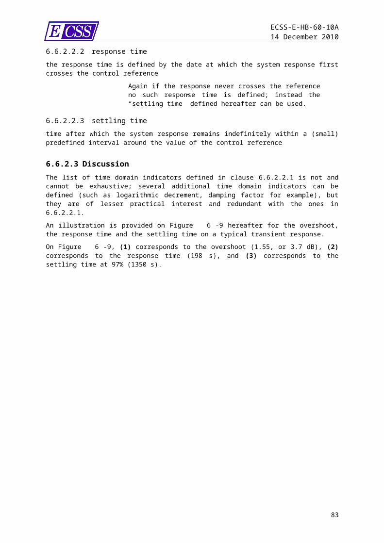
ECSS-E-HB-60-10A14 December 2010
The singular value of the output complementary sensitivity function determines the minimum modulus of the complex gain of the output feedback uncertainty that makes the system unstable.
NOTE For a SISO system the modulus margin determines the stability margins in the presence of a feedback uncertainty. It is therefore equivalent to the singular value of the complementary sensitivity functions (input or output being equivalent in SISO case).
The concept of sensitivity functions can be extended to more complex systems, for example involving nested control loops. The method for assessing the generalised stability margins for such system is:
to identify uncertainty against which to evaluate the stability margins, their position in the loop and their nature, to calculate the relevant sensitivity and complementary sensitivity functions, then to determine their singular values.
A.3.2 Analysis of stability margins – some illustrationsAn example of stability margins assessment for a continuous SISO system is given on Figure A-1 using the Nichols locus (single-axis attitude dynamics with one flexible mode, controlled by a first order phase-lead plus an elliptic low-pass filter):
Figure A-1: Example of gain and phase margins identification The proof of the closed-loop system stability was first given by computing the eigenvalues of the state matrix (all real parts are strictly negative).
83
ECSS-E-HB-60-10A14 December 2010
(1) corresponds to the gain margin (17 dB), (2) corresponds to the phase margin (28 deg); the modulus margin is 6.3 dB for this example, which means that the smallest modulus of complex feedback uncertainty that can drive the system unstable is 0.484. Figure A-2 illustrates a case with two gain and two phase margins (unstable plant controlled by a phase-lead with a pseudo-derivative filter and a second order low-pass filter). The rule for such a general system with multiple axis crossings is to define the stability margins properties from the four following values:
Positive gain margin: minimum value for all positive (20.5 dB in the example). Negative gain margin: minimum absolute value for all negative
(example 17.4 dB).
Positive phase margin: minimum value for all positive (example 29.1°). Negative phase margin: minimum absolute value for all negative (example 86.2°).
Figure A-2: A case with multiple gain and phase margins
84
ECSS-E-HB-60-10A14 December 2010
Annex BAppendices to clause 5:
Guidelines and mathematical elements
B.1 Error Indices with domains other than timeThe definitions given in clause 5.2 assume that the important quantity is the error variations over time, and hence the performance and measurement error indices are defined assuming that the domain variable is time. In some situations it can be more important to look at variation with respect to some other parameter, usually relating to position or orientation. For a more general domain variable, x, the indices can be redefined as follows:
Where is a specified region of parameter space and means that x lies within that region.
NOTE 1 The parameter space should be defined in the requirements according to what is being constrained, analogously to choosing the time interval as described in B.2.NOTE 2 For the PSE it is necessary to specify the vector x, and to say how x – x should be interpreted (e.g. whether direction of x is fixed or not.)NOTE 3 The Performance Drift Error (PDE) has not been redefined, as for a non-time domain it is indistinguishable from the PRE.
85
ECSS-E-HB-60-10A14 December 2010
NOTE 4 The knowledge error indices can also be redefined similarly for the spatial case.
B.2 Considerations regarding time intervalsThe error indices given in clauses 5.2.3 and 5.2.4 generally depend upon one or more time intervals t. (Except for APE, AKE.) The choice of t is driven by the properties to be constrained for the system in question. Usually there are natural timescales: for example, the integration time of a sensor, the time spent on a single observation, the time between recalibration events. This also applies for the interval t used in the PSE index. The tables in annex B.3 give some guidelines as to which timescales to select for use in a given index, based on what that index is being used to constrain.A less obvious consideration is how to deal with the ensemble of such intervals. Should a requirement be for the worst possible interval, an average interval, or for a fraction of intervals? This is something which should be considered when defining the statistical interpretation to be used for a requirement, as described clause 5.3.4.In some cases, there is a finite number of possible time intervals in the ensemble (e.g. a spacecraft which makes an observation then moves on to another target). In others, there is an infinite set of time intervals which can theoretically be used (e.g. taking a single long observation for many times the length of the sensor integration time).
B.3 Relationship between error indices and physical quantities
The error indices defined in clauses 5.2.3 and 5.2.4 are used instead of common terms such as bias or stability, as these terms can be misleading due to alternative definitions being used in different contexts. The word “stability” in particular has several alternative definitions. However the indexes can seem abstract, and especially once the statistical interpretation is included it can be hard to relate these to physical, well understood, quantities. The following table lists different types of quantities that can need to be constrained, for a given system or mission, and gives the appropriate choice of performance error index, timescales and statistical interpretation. This list is not comprehensive, as each system needs to be analysed independently, but is intended to give an overview of how fundamental needs are translated into performance error requirements of the type discussed in clause 5.
NOTE 1 In this context, “mission” refers to the total duration for which the system is operatingNOTE 2 In this context, “observation” refers to a period during which the system has a single target (or more generally target trajectory)NOTE 3 For explanation of the statistical interpretation refer to clause 5.3.4NOTE 4 Knowledge errors can be treated similarly
86
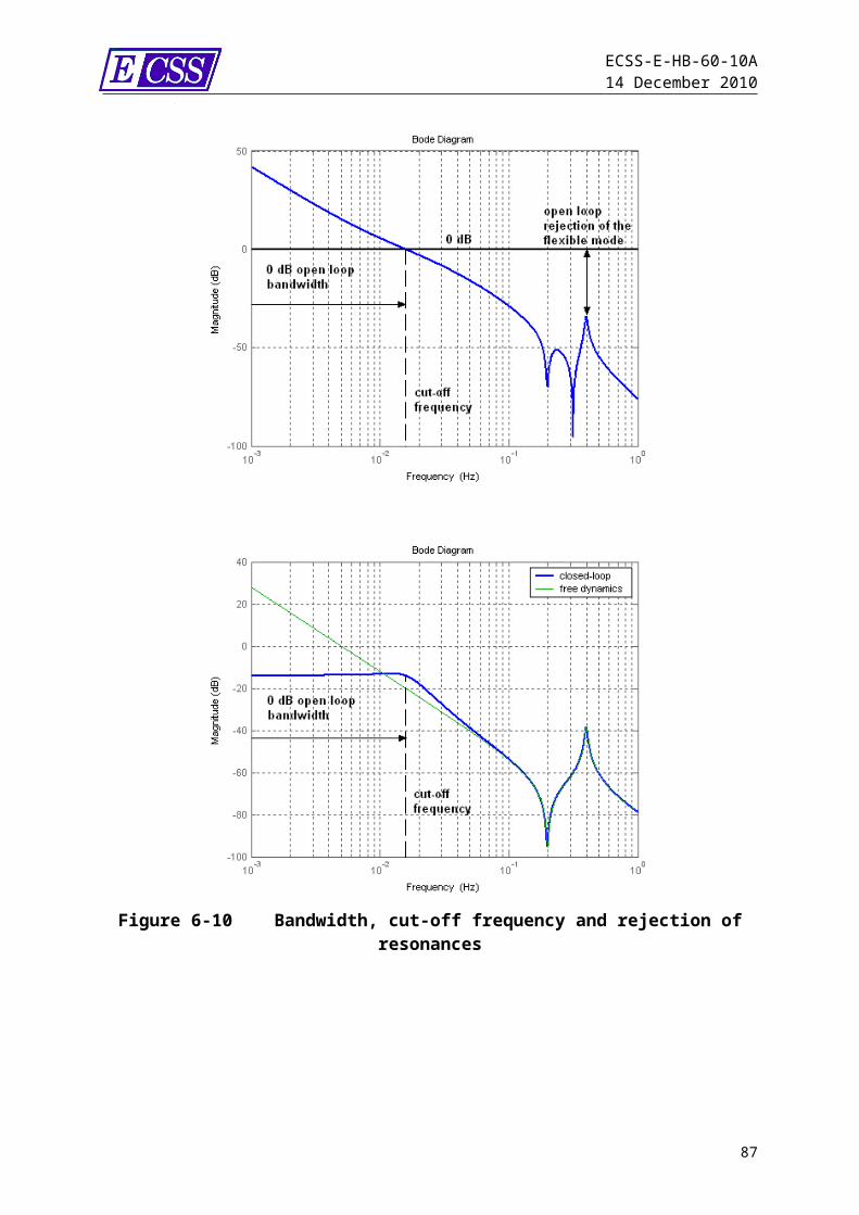
ECSS-E-HB-60-10A14 December 2010
Table B-1: Types of performance quantities, and the error indices used to constrain them
Property to be constrained Index Used
Timescale(s) Statistical interpretation
Maximum deviation from target (i.e. worst case time)
APE - Ensemble of SC and/or intervals
Fraction of time allowed outside a specified bound
APE - Temporal
Bias during an observation MPE Observation duration
Ensemble of SC and/or observations
Fraction of observations with bias above a specified bound (worst case SC)
MPE Observation duration
Ensemble of observations
Bias over the mission lifetime MPE Mission lifetime Ensemble of SCMaximum allowed change in the error during an observation (worst case)
PSE t=observation duration
Ensemble of SC and/or observations
Number of observations for which change in error exceeds upper bound
PSE t=observation duration
Temporal
Maximum deviation from the mean during an observation (worst case)
PRE t=observation duration
Ensemble of SC and/or observations
Fraction of time spent more than a certain amount away from the mean pointing during integration time of a sensor
PRE t=integration time
Temporal
Maximum pointing drift over mission PDE t=time to average short-term errorstPDE=mission duration
Ensemble of SC
Maximum allowed performance drift during a long observation
PDE t=time to average short-term errorstPDE=observation duration
Ensemble of SC and/or observations
Number of observations for which the drift exceeds a given value
PDE t=time to average short-term errorstPDE=observation duration
Temporal
Maximum allowed deviation (compared to the first observation) when attempting to repeat an observation at a alter time
PRE t=observation durationtPRE=time between observations
Ensemble of SC and/or observations
Number of repeat observations for which the mean deviation exceeds a given bound compared to the first observation
PRE t=observation durationtPRE=time between
Temporal
87
ECSS-E-HB-60-10A14 December 2010
observations
B.4 Statistics for Monte Carlo Minimum Number of RunsConsider a requirement P(x<xmax,)>Pmin, with some statistical interpretation. This means that for the system to meet its requirement:
In any given trial the probability of having x < xmax shall be at least Pmin. Or equivalently,
The probability of having a failure (x > xmax) in any given trial shall be less than Pf
max=1-Pmin.Given a Monte Carlo campaign with N runs, of which nf of these are failures. Assuming that the real underlying probability of failure (not know to the experimenter) is P f, then the probability of observing nf failures in N trials is given by the binomial formula:
If there is no a-priori information about the value of Pf, then for a given number of observed failures nf the probability distribution of Pf is found (using the expression
) to be
If the requirement is met, the probability of failure is less than some value P fmax. (NB this
is equivalent to a minimum required probability of not failing the requirement.) Given n f
failures in N trials, the confidence of the requirement actually being met (i.e. of Pf really being less than Pf
max) is:
Where inc is the incomplete beta function, chosen to agree with the built in MATLAB definition. Using this formula, it is possible to work out the number of runs required in order to meet a requirement with a specified probability to a given confidence level. See Table 5-11 in subclause 5.4.3.3.An alternative formula often seen in the literature is for the minimum number of runs required to required to estimate the position of the confidence level:
Where N is the minimum number of runs required to estimate the PC level of a distribution, such that there is an nC- confidence that the real value of PC it a level x=xC
is within the range PCest± P.
Which formula is appropriate depends upon the context, but generally it takes more samples to estimate a confidence level than to prove that the failure rate is acceptable.
NOTE For example, if the requirement is specified at 99.73%, then 11964 samples are needed to estimate this confidence level with a 95% confidence of the real
88
ECSS-E-HB-60-10A14 December 2010
value being within ±0.1% of the estimate. However assuming no failures are seen, only 1108 runs are required to prove that the probability of failure is <0.27% to a 95% confidence.
B.5 Determining the error PDFs
B.5.1 OverviewThis clause splits errors contributing to a budget into different classes, according to their type of variation over time. It looks at how to assign PDFs to these errors, based on the index being assessed and the statistical interpretation of the corresponding requirement. For each index (APE, MPE, etc) we require the probability distribution of a different quantity:
For APE we require the distribution of , the error value over time
For MPE we require the distribution of , the mean error over a period t
For RPE we require the distribution of , the difference between the error at a time t and its mean value over a period t
For PSE we require the distribution of , the difference between the error at a given time and the error at a time t earlier, where t is fixed
For PDE we require the distribution of , the difference between two averages over periods (within the same observation) separated by a time tPDE
For PRE we require the distribution of , the difference between two averages over two different observation periods separated by a time tPRE
In most cases it is not necessary to know the full distribution, as if approximate methods are being used (clause 5.5) then only the mean and variance of the distribution are needed. These are defined in terms of the PDF P() using the formula:
Clauses B.5.2 to B.5.9 give some simplified formulae for obtaining the means and variances for the above index quantities, for the most common cases. In many cases there are no simple formulae, and the only solution is to perform a more detailed analysis on the error.
NOTE Only performance error indices are considered, however the extension to knowledge error indices is trivial.
B.5.2 White noiseWhite noise has a Gaussian distribution with zero mean. In reality pure white noise never occurs, however it is a very good approximation to many situations.
89
ECSS-E-HB-60-10A14 December 2010
NOTE In many cases (e.g. sensor noise) the standard deviations are directly specified (manufacturers data), and it is not necessary to assess the distributions.
Since there is no upper bound to a Gaussian, to assess “ensemble” distributions it is conventional to impose one at the 3 level. In this case the ensemble parameter (see annex B.5.9) is the standard deviation. To describe the ensemble distribution we need to refer to “the standard deviation of the standard deviation”, which is mathematically well defined but can be confusing.
Table B-1: Means and standard deviations used for white noise errorsIndex S.I
.Distribution NotesP() () ()
APE E 3s 3s See note. For P(s), s and s see B.5.9
T G(0,sWC2) 0 sWC
G(,V)= Gaussian with specified mean & variance, sWC =worst case s
M 0 sOr use manufacturers data. For s see B.5.9
MPE all 0 0 0 Zero mean so no MPE contributionRPE As for APE Zero mean so RPE identical to APEPDE All 0 0 0 No change over timePRE All 0 0 0 No change over timeNOTE: Since there is no upper bound to a Gaussian, it is conventional to impose one at the 3
level (see text).
B.5.3 Biases A bias error is constant, either over the entire mission or over the observation period in question. The temporal distribution is therefore a delta-function, while the ensemble distribution can take different forms: see annex B.5.9.
Table B-1: Means and standard deviations used for bias errorsIndex S.I
.Distribution NotesP() () ()
APE E P(B) B B For P(B), B and B see B.5.9.T (BWC) BWC 0 BWC=worst-case biasM P(B) B B For P(B) see B.5.9.
MPE As for APE MPE same as APERPE All (0) 0 0 No contribution by definitionPDE All (0) 0 0 No contribution by definitionPRE E P(B) 0 2½B See note
T (Bmax-Bmin) Bmax-Bmin 0 See noteM P(B) 0 2½B See note
NOTE: By definition biases do not contribute to the RPE and PDE indices. They contribute to the RPE index in the case where biases change between observations. In such cases P(B) can be difficult to assess (used for E,M interpretations), but the approximation ≈ 2½B is generally good enough
90
ECSS-E-HB-60-10A14 December 2010
B.5.4 Uniform random errorsUniform random errors are those vary over a short timescale, with a probability distribution uniformly distributed in a given range. (i.e. zero probability of occurring outside this range.) Such errors are appropriate e.g. for rounding errors, errors from a bang-bang controller. Table B-1 assumes that the range of the error is 0-C. Depending on the situation the bound C can be a fixed value, a worst case value or an ensemble parameter (see annex B.5.9). It is easy to modify the table for other error ranges (e.g. –C/2 to +C/2) if required.
Table B-1: Means and standard deviations used for uniform random errors
Index S.I. Distribution NotesP() () ()
APE E P(C) C C For P(C), C and C see B.5.9.T U(0,CWC) U(xmin,xmax)=uniform in range
xmin to xmax. CWC=worst case CM For C and C see B.5.9.
MPE E For P(C), C and C see B.5.9.
T 0 CWC=worst case C
M For P(C), C and C see B.5.9.
RPE E For P(C), C and C see B.5.9.
T 0 U(xmin,xmax)=uniform in range xmin to xmax. CWC=worst case C
M 0 For P(C) and C see B.5.9.
PDE All 0 0 0 No contribution as timescale of variation too small
PRE All 0 0 0 No contribution as timescale of variation too small
B.5.5 Harmonic errorsHarmonic errors are those which have a sinusoidal variation over time. This clause considers only errors with zero mean, = A sin(2t/T), where T is the period. Errors with non-zero mean can be considered as a combination of a harmonic error and a bias. A can be a fixed value, a worst-case value or an ensemble parameter. There are generally two cases, T << T and T >> T, where T is the averaging timescale used in the indices APE, MPE, etc.
91
ECSS-E-HB-60-10A14 December 2010
Table B-1: Means and standard deviations for low period (T << T) harmonic errors
Index S.I. Distribution NotesP() () ()
APE E P(A) A A For P(A), A and A see B.5.9.T
0 AWC=worst case A
M 0 For P(A), A and A see B.5.9.
MPE all 0 0 0 No MPE for low period errorsRPE all As for APE No mean so RPE, APE samePDE all 0 0 0 No change over time so no
contribution to PDE, PREPRE all 0 0 0
Table B-2: Means and standard deviations for high period (T>>ΔT) harmonic errors
Index S.I. Distribution NotesP() () ()
APE E P(A) A A For P(A), A and A see B.5.9.T
0 AWC=worst case A
M 0 For P(A), A and A see B.5.9.
MPE all As for APE Low period implies no significant change in the error during an averaging timeRPE all 0 0 0
PDE E 2A 2A Actual values depend on the definitions of PDE, PRE. These values are computed assuming a worst case where the 2 intervals are taken ½ period (time T/2) apart, so that δε=2ε
T 0
M 0PRE all As for PDE
B.5.6 Drift ErrorsA drift error has a linear variation with time, = Dt, where D is the drift rate. It is assumed that the drift is reset at intervals TD (e.g. after each observation). Depending on the context, the drift rate D can be a single value, a worst case or an ensemble parameter.The reset timescale TD is assumed to be greater than or equal to the timescale used for averaging in the MPE and RPE indices: TD T. For the PDE index it is assumed that TD>TPRE>>T.The drift need not be reset to the same value each time: however this should be dealt with as a separate bias error, see clause B.5.3.
92
ECSS-E-HB-60-10A14 December 2010
Table B-1: Means and standard deviations for drift errorsIndex S.I. Distribution Notes
P() () ()APE E TDD is the worst
case drift before resetting occurs, for a given value of D. DWC is the worst case D. For P(D), D and D see B.5.9.
T U(0,TDDWC)
M
MPEE
Note that TD T, so that max MPE for given D is T
M
RPE EFor given value of D, RPE range is T 0
M 0
PDE E/M Note that TD>TPRE>>T
T Temporal interpretation does not applyPRE all 0 0 0 No contribution by
definition
B.5.7 Transient Errors In this context, transient errors refers not to initial settling effects, but to situations where the normal operation is disrupted by a specific event (for example STR loss of tracking), after which there is a period of degraded performance before normal performance levels are reached again. Such errors are difficult to characterise, because of their temporary (and often unpredictable) nature, but they are part of a performance budget. In general the best way to handle such errors is to create a histogram, of expected deviations versus probability of occurrence. Depending on the statistical interpretation a different histogram is used:
Ensemble requirements: the histogram is of the maximum values for different members of the statistical ensemble versus the probability of such an ensemble occurring:
Temporal requirements: the histogram is of the possible values (up to the maximum) as a function of the probability of having that value at a random time:
93
ECSS-E-HB-60-10A14 December 2010
Mixed requirements: the histogram is of the possible values as a function of the probability of having that value at a random time and for a random ensemble member
NOTE To avoid excessive contributions to budgets, it can be desirable to produce two separate budgets: one with and one without transient contributions. In some cases two separate sets of requirements can be given for nominal cases and with transients.
Table B-1: Means and standard deviations for drift errors
Index S.I.Distribution
NotesP() () ()
APE E
-T
M
MPE all 0 0 0 Assuming low probability of transient event, there is no significant effect on the mean
RPE all As for APE
B.5.8 Others (General Analysis Methods)The previous clauses consider the most common types of errors used in a spacecraft performance budget. Other types of time variation are possible (random walk, non-sinusoidal periodic error, etc.). If error data is available then it can be used directly in the budget. If not, a prerequisite is to analyse the effect to determine its behaviour, and hence its statistics. There are two ways to analyse a general effect in order to extract the quantities required to produce a budget:
Analysis by time behaviour For the ensemble interpretation, the PDF required is that of the maximum error max across the ensemble. The PDF P(X) of the ensemble parameter X is obtained using the methods of clause B.5.9. If the maximum value of the error is a function of X, max=max( (X), then the mean and standard deviation is given by
If max=CX then this simplifies to max)=C(X), max)=C(X) For the temporal interpretation, the PDF required is that of the probability of finding a specific value of for a given value of X (the worst case). If there are clear bounds to the error, , then
94
ECSS-E-HB-60-10A14 December 2010
Where CN is a normalisation constant. This expression is derived from the expression
For the mixed interpretation, the PDF to be used is the probability across all times and all ensemble members
Where P(X) and P(|X) are found as described above. Alternatively the mean and standard deviation can be found as functions of those for a given X
Note that although the above discussion assumes only a single ensemble member it can be extrapolated to more parameters.
Analysis by histogram: in some cases it can be more appropriate to bin the possible values of the error into a histogram, from which the mean and standard deviation can be extracted using the formulae:
,
See clause B.5.8 for comments on the appropriate choice of histogram.
B.5.9 Distributions of Ensemble ParametersIn clauses B.5.2 to B.5.8 the error statistics (in ensemble or mixed interpretations) depend on the statistics of the ensemble parameters (A, B, C, D, s). For a general ensemble parameter, X, we need to be able to determine the probability distribution of X given the data available, and in particular the mean and standard deviation of its distribution.
Case 1: measured data. If a measurement is made of the parameter X, this gives a measured value plus some error range, Xest±X, where X corresponds to the n- level of a Gaussian. In this case the appropriate distribution is a Gaussian with:X=Xest, X= X /nThis is appropriate for for the measured bias of a sensor. Case 2: bounds known, distribution not known. If it is known that X is in the range Xmin to Xmax, and that intermediate values are possible, but no other information is available, then the appropriate distribution is a uniform distribution between these bounds. In this case the mean and standard deviation are given by:
,This is appropriate for example for alignment using shimming. Case 3: PDF of ensemble parameter known. In such case the mean and variance can be extracted directly from the probability distribution. Table B-1 gives means and variances for some common distributions:
95
ECSS-E-HB-60-10A14 December 2010
Table B-1: Some common distributions for ensemble parametersDistribution Parameters
Name Form Mean VarianceGeneric PDF P(x)
Gaussian 2
Uniform Distribution
Typical Bimodal(PDF for sinusoid)
Beta Function(NB a, b>1)
if , zero otherwise
Symmetric Beta Function
if , zero otherwise
Symmetric Truncated Gaussian
B.6 Mathematics of an Error Budget
B.6.1 Probability distributions and the statistical interpretationAn error budget is a means of estimating the probability distribution of an error index applied to an error, I(e), where e is a combination of several contributing error terms e=c11+…+ cN N. Before the probability distribution P(I) can be estimated, it needs to be clear exactly what distribution is being assessed: this depends on the statistical interpretation of the requirement.For illustration, consider a single contributing error which is a function of time, t, and of a single ensemble variable A: .
An index I applied to this error is therefore also a function of t and A, and possibly also of one or more time intervals t.
96
ECSS-E-HB-60-10A14 December 2010
If the parameter A is known or specified, then the probability distribution (PDF) of is , where P(x|y) denotes “the probability of finding value x if y is true”, and
similarly for the index I: .
The parameter A is not generally known exactly, but has some range of possible values, described by a PDF, P(A).
When making a requirement of the form , it is necessary to specify what the statistical interpretation is. Depending on this, the correct PDF to assess in the requirements is chosen:
Temporal Interpretation. This applies to requirements of the form:“The requirement shall be met for P% of the time for all possible combinations of ensemble parameters”. In order to verify the requirement for all ensemble parameters, Ai is set to the value giving the worst case.
,
Depending upon the form of the function the value of A giving the worst case error can be or not its maximum value. Ensemble Interpretation. This applies to requirements of the form: “The requirement shall be met at all times for P% of the possible combinations of ensemble parameters”. In order to verify such a requirement, t is set to the value giving the worst case error:
,
In the case that , where , then Mixed Interpretation. This applies to requirements of the form “The requirement shall be met at all times for P% of the possible combinations of time and ensemble parameters”. To verify such a requirement, it is important to cover all possible combinations of t and Ai:
NOTE The time interval(s) t do not appear in the above expressions: depending upon the context (i.e. on how the requirement is framed) it can be appropriate to treat them as temporal or ensemble variables.
B.6.2 Exact error combination methodsSuppose that the total error is a linear sum of contributing terms, error to be a linear sum of N contributing terms, , and that I is one of the indices defined in 5.2. It is possible to show that the index applied to the total error is the sum of the index applied to the contributing terms
This is abbreviated to .
97
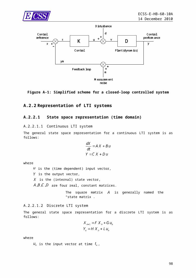
ECSS-E-HB-60-10A14 December 2010
The probability distribution of the total error IT is obtained by combining the probability distributions of the individual terms Ii. (See annex B.5 for discussion of how these are obtained.) The integral is:
From this, the probability of the requirement being met can be shown to be:
Where is the function defined such that:
(Note that normalisation terms are omitted for simplicity.)For all but the most trivial cases this is not integrated exactly, but is done either by numerical integration or by Monte Carlo methods. Alternatively, approximate techniques can be applied.This expression can be generalised to the case where IT is a non linear combination of I1, I2,…IN:
However for this case the relationship between IT and the contributors I1 to IN does not necessarily follow directly from the relationship between etotal and the contributing errors e1 to eN.
B.6.3 Alternative approximation formulaeMany different approximate summation rules can be found in the literature, especially where spacecraft pointing errors are concerned. In particular, the ESA Pointing Error handbook gave three options for summation rules:
Where S, LT and ST denote three temporal classes (see clause 2_5.2 of the ESA Pointing Error handbook EHB.DGD.REP.002, 19 Feb 1993). The first of these is equivalent to applying the pure Gaussian summation rules, and is equivalent to rules in clause 5.5.4, providing that there are no correlated errors. The alternative summation rules (the second and third of the three above equations) are attempts to modify the Gaussian summation law in order to make it more conservative. The rationale for this was that, if the variance was estimated using the method of bound/3, then this was likely to be an underestimate of the true variance, and so a way of overestimating the total variance was needed to compensate.Although these rules have been used successfully for many missions, they have caused much confusion. In particular, they cannot be rigorously justified, except on the basis of working in practice. There is also no way of choosing one over the other to be preferred. For these reasons, this document discourages their use. Instead, if more accurate methods are used to estimate the contributing variances, as described in annex B.5, then there is no need to adapt the Gaussian summation laws to give a more conservative estimate.
98
ECSS-E-HB-60-10A14 December 2010
Annex CSatellite AOCS case study
C.1 IntroductionThis annex aims at illustrating the budget computation presented in clause 5 for the specific case of the pointing performance of an Earth observation satellite. The example is not exhaustive in terms of pointing requirements and contributing errors which depend strongly on the mission and the payload used, but focuses on the most important ones for that type of mission: the absolute pointing and knowledge requirement, and the stability requirement.
C.2 Satellite AOCS architectureThe example is based on Earth observation satellite on a Low Earth Orbit. The satellite is three axes stabilised in mission mode. Its AOCS architecture is based on star sensor and gyro attitude measurements, combined through an attitude estimation filter, reaction wheels for torque control, and magnetotorquer bars actuation for wheels kinetic momentum unloading.The satellite flexible solar arrays are rotating thanks to Solar Array Driving Motors (SADM). The imaging payload line of sight is moved by a steerable mirror.
C.3 From Image quality to AOCS requirementsThe most important requirements concern the acquisition of the image as illustrated on Figure C-1 for SPOT 5 satellite.To get a good image quality, i.e. a precisely aimed one with a minimum of distortion between its composite elements, it is necessary:
To ensure accurate average pointing of the instrument’s optical axis. The pointing performance (given at System level) Asystem_1 of the optical axis determines the usable instrument field of view. To have a good knowledge Asystem_2 of this pointing characteristic enabling accurate knowledge location of the targeted points, To keep the instrument stable during imaging. This means having very low angular velocities to avoid image distortion or bad registration of the pixels. This stability requirement becomes a constraint on the angle to be held for a certain time DT.
99
ECSS-E-HB-60-10A14 December 2010
Figure C-1: Images are taken by scanning with a CCD array detector (SPOT 5)
Figure C-2 shows an example of maximum pointing and stability error. Within the observation duration (here 300s), all the performance requirements (pointing and stability) are applicable. On that plot, the stability error is defined as the maximum peak-to-peak variation of the attitude during the time period DT.
Figure C-2: Example of Pointing error and stability error over DT=10s
100
ECSS-E-HB-60-10A14 December 2010
Two time scales are taken into account where stability is concerned: a short time horizon depending on the time needed to integrate the pixels of the image line; a stability error Asystem_3s during this time DTs leads to a radiometric degradation of the image and a variation in the sampling step for the image on the ground. a longer time horizon depending on the time needed to scan part of the image. A stability error Asystem_3l during this time DTl causes geometric distortion of the image seen as distortion of the lines (Figure C-3):
Figure C-3: Geometric image distortion: altering the linesThe satellite’s pointing and stability specifications come from image quality specifications at System level.aaa. The performance allocation at Satellite level Asat is derived from the one at System
level Asystem by considering other contributions from the payload (internal characteristics and errors) and ground (image post-processing, etc.). Then the performance allocation for the AOCS AAOCS is derived from those at Satellite level by subtracting contributions from other satellite subsystems (for example, misalignments or residue of calibration, thermoelastic disturbances between payload and attitude sensors, depending on the project). For example, the AOCS specifications derived from image quality can be:1. Pointing error AAOCS_1 < 0.05° for each axis of the satellite, for 99.7% of the
scenes and of the satellite dispersions.2. Attitude determination error for image quality: AAOCS_2<0.005° for each axis of
the satellite, for 99.7% of the scenes and of the satellite dispersions.3. Long term stability error AAOCS_3 < 5.10-3° during DTl=10s for each axis of the
satellite, for 99.7% of the scenes and of the satellite dispersions.4. Short term stability error AAOCS_4 < 5.10-5° during DTs=10ms for each axis of
the satellite, for 99.7% of the scenes and of the satellite dispersions.NOTE It is important that the wording of the requirement is very precise, in particular concerning the stability issue with respect to the mission needs. FigureC-4 illustrates a special case where the requirement on the stability error can produce very different results. Let us assume that the stability error is defined as a the peak-to-peak variation over the time frame. If the requirement is expressed as the maximum value of the stability error over the whole observation period, then obviously the result is around 1. If it is expressed as the maximum value, but only over 99.7 % of the observation period (3), then the result is around 0.1.
101
ECSS-E-HB-60-10A14 December 2010
Figure C-4: stability error examplebbb. For robustness purpose of the AOCS, some requirements can be added, that can be
seen as “engineering rules”, for example stability margins (gain, phase, delay, module), to be satisfied in spite of satellite dispersions (inertia, flexible modes damping ratio and frequency, sensor and actuator delays, etc.). For example, a stability margin requirement can be expressed this way:1. The stability margins are 6 dB and 30 degrees minimum for 66% of satellite
dispersions2. The stability margins are 3 dB and 15 degrees minimum for 99.7% satellite
dispersionNOTE This requirement implies that the control loop remains stable for any satellite dispersions but with reduced margins, taking into account that the satellite dispersions from 66% to 99.7% hide the missing margin from requirement 5 to 6.
C.4 Formulation of the requirements C.3aaa1 to C.3aaa4 using error indices
C.4.1 GeneralIn this clause, requirements 1 to 4 are reworded according to clause 5, using error indices and statistical interpretation.Let us recall the principle:
A performance requirement for some system should expressed by giving an upper bound, Imax, for some quantity, expressed as an error index I(eP), together with a probability that the index lies within this bound.
Expressed mathematically:
102
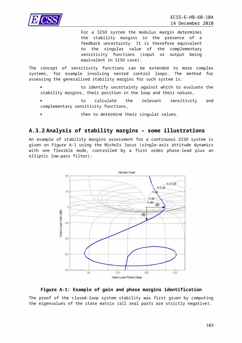
ECSS-E-HB-60-10A14 December 2010
It is important that the following elements are present to ensure that the requirement is clear, complete and unambiguous:a. The exact definition of the property to be constrained. To define this, the following
is necessary:1. The choice of error function eP
2. The index to be applied to this function, I(eP)b. A maximum allowed value for this index, Imax.c. The required probability, PC, that the index is inside the allowed ranged. The conditions under which the probability is to apply (known as the “statistical
interpretation”)
C.4.2 Choice of signal error function The AOCS specification is expressed in terms of difference between the Euler angles with respect to a reference frame. Thus Euler angles are the adequate error function for pointing and stability requirements. For sake of simplicity, they are denoted (t).
C.4.3 Choice of error indices and maximum valuesThe pointing requirement C.3aaa1 can be expressed using the Absolute Performance Error (APE). APE denotes the instantaneous value of the performance error at a given time. The maximum value for this index is AAOCS_1 = 0.05 deg.The attitude determination requirement C.3aaa2 can be expressed using the Absolute Knowledge Error (AKE). AKE denotes the instantaneous value of the knowledge of the error at a given time. The maximum value for this index is AAOCS_2 = 0.005 deg.The stability requirements C.3aaa3 and C.3aaa4 can be expressed using the Performance Stability Error (PSE). PSE denotes the difference between APE at the given time t and APE at t-dt, where dt is a given time interval. The maximum value for this index is
AAOCS_3 = 0.005 deg over 10s for long term stability AAOCS_4 = 5.10-5 deg over 10 ms for short term stability
C.4.4 Assigning a probability density function (PDF)The probability density function is related to the type of error sources contributing to each requirement (see clause C.6). Each error source has its own PDF and the total error PDF is the combination of them. Only for trivial cases, the combination of several PDFs is a complex mathematical task which is performed numerically. For analytical budget computation, an approximate method is used, considering only the contributors mean and variance, which can be easily summed at the end to compute the total error mean and variance (or standard deviation).In our case, all requirements are expressed for 99.7% of time and spacecraft dispersions; the standard deviation (times 3) of the total error is compared to the index maximum value.
103
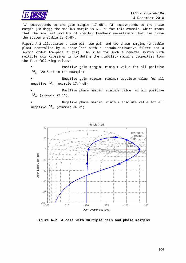
ECSS-E-HB-60-10A14 December 2010
C.4.5 Choice of statistical interpretation (temporal, ensemble, mixed…)All the requirements apply for temporal interpretation (99.7% of scenes, i.e. 99.7% of mission duration) and ensemble interpretation (99.7% of satellite dispersions), each one bound limited (thus it is a “modified” interpretation). In absence of detail they are of “modified mixed statistical interpretation”.
NOTE The requirements can also be expressed so that one interpretation becomes dominating. For example, the pointing requirement can be detailed as follows:
R11: pointing error AAOCS_1 < 0.05° for each axis of the satellite, for 99.7% of the scenes and 15% satellite dispersions around the nominal. R12: pointing error AAOCS_1 < 0.07° for each axis of the satellite, for 99.7% of the scenes and 30% satellite dispersions around the nominal.
For R11, the time interpretation is dominating, for R12, it is the ensemble interpretation.
C.4.6 Requirements formulationThe requirements formulation elements are recalled on Table C-1. Then the relations in C.4.6.1Table C-2 are relevant
Table C-1: Requirements formulation elementsRequirement Signal
error function
Error index
Statistical interpretatio
n
Index maximum
valueR1 pointing accuracy Euler angles
(t)APE Modified Mixed 0.05 deg
R2 attitude determination
Euler angles (t)
AKE Modified Mixed 0.005 deg
R3 short term attitude stability over time
Euler angles (t)
PSE Modified Mixed 5.10-5 deg over 10 ms
R4 long term attitude stability over time
Euler angles (t)
PSE Modified Mixed 0.005 deg over 10s
104
ECSS-E-HB-60-10A14 December 2010
Table C-2: Temporal requirements formulationCommon wording Standard wording
Pointing error AAOCS_1 < 0.05° for each axis of the satellite, for 99.7% of the scenes and of the satellite dispersions
“The absolute value of the APE of Euler angle between satellite frame and reference frame on each axis shall be less than 0.05 deg for 99.7% of time and 99.7% of satellite dispersions” (modified mixed interpretation).Prob ( |APE((t))|) < 0.05° ) > 0.997
Attitude determination error for image quality: AAOCS_2<0.005° for each axis of the satellite, for 99.7% of the scenes and of the satellite dispersions
“The absolute value of the AKE of Euler angle between satellite frame and reference frame on each axis shall be less than 0.005 deg for 99.7% of time and 99.7% of satellite dispersions” (modified mixed interpretation).Prob ( |AKE((t))|) < 0.005° ) > 0.997
Long term stability error AAOCS_3 < 5.10-3° during Tl=10s for each axis of the satellite, for 99.7% of the scenes and of the satellite dispersions
“The absolute value of the PSE over 10s of Euler angle between satellite frame and reference frame on each axis shall be less than 0.005 deg for 99.7% of time and 99.7% of satellite dispersions” (modified mixed interpretation). Prob ( |PSE((t,dt))|) < 0.005° ) > 0.997, 0<dt10s
Short term stability error AAOCS_4 < 5.10-5° during Ts=10ms for each axis of the satellite, for 99.7% of the scenes and of the satellite dispersions
“The absolute value of the PSE over 10ms of Euler angle between satellite frame and reference frame on each axis shall be less than 5.10-5 deg for 99.7% of time and 99.7% of satellite dispersions” (modified mixed interpretation).
Prob ( |PSE((t,dt))|) < 5.10-5°) > 0.997, 0<dt10ms
C.5 Formulation of requirements C.3bbb1 and C.3bbb2Requirements C.3bbb1 and C.3bbb2 deal with the control loop stability margins. For this type of requirements no error function or error index is defined.The requirements are typically of ensemble interpretation, because they are only linked to satellite dispersions. No standard wording is proposed for this type of requirements. The common wording is relevant.
C.6 Control Performance verification principles
C.6.1 Choice of verification method Depending on the phase of the project, several verification methods can be used:
Analysis (error budget, Black-Nichols diagrams, etc.)
105
ECSS-E-HB-60-10A14 December 2010
Simulation (Monte-Carlo simulations, etc.) Experiment (on ground testing, in flight results, etc.)
In this clause, only the error budget computation is detailed.
C.6.2 Compiling the error budget (requirements C.3aaa1 to C.3aaa4)
C.6.2.1 GeneralThe computation of the error budget with respect to one performance requirement can be decomposed into three steps:a. Identification of the contributing error sources (type and statistical characteristics)b. Computation of each error source contribution to total errorc. Computation of the total error and comparison to the requirement
C.6.2.2 Step 1: Identification of error sourcesThe error sources nature depend on the control loop elements (sensors, actuators, controlled system, electronics), its environment (external disturbances, on/off, etc.) and the requirement to be met: for example a bias error source has no contribution to RPE (which is the variation to the mean value), but it contributes to the MPE (mean value). The list of error sources (not exhaustive) relative to our example is detailed in clause C.7. This clause is focused on the type or the error and its PDF. According to Annex B.5 the error sources can be classified as shown in Table C-1.
106
ECSS-E-HB-60-10A14 December 2010
Table C-1: Error sources classesError class Comments Error index to
which it contributes
White noise (WN class)
Not physical, but good approximation of real noises (sensors for example)
APE, AKE, RPE, RKE, PSE, PSKE
Gaussian, zero mean, standard deviation
Uniform random (UR class)
random errors which vary over a short timescale (quantization for example)
APE, PKE, MPE, MKE, RPE, RKE, PSE, PSKE
Uniform distribution [0-C], mean C/2, standard deviation C/(12)1/2
Bias (B class) Constant over the observation period. Mean value of harmonic errors and white noises.
APE, AKE, MPE, MKE, PRE if bias changes between two observation periods
Maximum (worst case) value
Harmonic (H class) Sinusoidal variation over time with zero mean, period T
APE, AKE, RPE, RKE, PSE, PSKEMPE, PDE depending on the period duration T with respect to the observation period
Max value A, standard deviation A/(2)1/2
Drift (D class) linear variation with time (slope D), observation period To
APE, AKE, MPE, MKE, RPE, RKE, PDE, PSE, PSKE
Mean value DTo/2Standard deviation DTo/(12)1/2
Transient (T class) Operation disturbance by specific event (star tracker loss of measurement for example). Does not apply to transient due to initial conditions.
APE, AKE, RPE, RKE, PSE, PSKE
Histogram of occurrences,See Annex B.5.7
Others (O class) random walk, non-sinusoidal periodic error
Depends Depends
C.6.2.3 Step 2: Computation of error contribution To compute the error contribution to the budget, the linear (or linearised) transfer function between the error source and the performance error of interest is computed. Assuming this linear behaviour, the contribution of one error source to the budget is of the same class as the error source, and thus has the same PDF assignment and its statistical characteristics can be computed from the error source ones and the transfer function gain. In particular, a noise source transforms into a noise contribution and a harmonic source into a harmonic contribution.The computation of the error contribution can be decomposed into three steps:
107
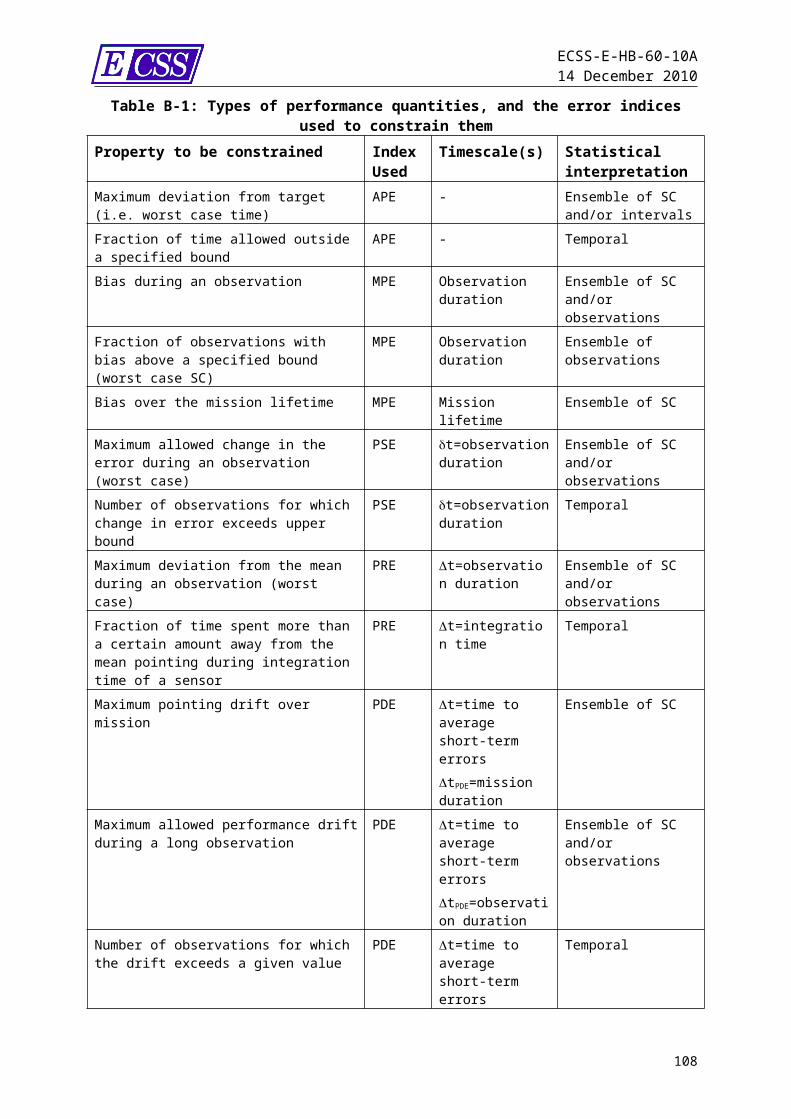
ECSS-E-HB-60-10A14 December 2010
a. Identification of the linear (or linearised) transfer function between the error source and the performance error. Several techniques can be used to perform this (linear modelling, system identification, linearization, etc.). They are not be described here.
b. Computation of the performance error signal statistical characteristicsc. Application of the error index to the performance errorLet us detail steps C.6.2.3b and C.6.2.3c.
Step C.6.2.3b: Computation of the performance error signal statistical characteristics Let e(t) denotes the error source and (t) the performance error. They are linked by the following transfer function (s) = H(s) e(s), where s denotes the Laplace variable. The following computation rules apply:
Harmonic errors (including bias, assimilated to harmonic with zero frequency)
o Temporal domain: The sine error e(t) = A sin (2f0t) is transformed by the linear transfer function H into a sine (t) at the same frequency f0, of amplitude B=|H(f0)|A and with phase lag (f0), where |H(f0)| is the gain of the transfer function H and (f0) its phase at f0.
e(t) = Asin(2f0t) (t) = |H(f0)|A sin(2f0t+(f0))
o Frequency domain: The maximum value of the harmonic contribution (t) at frequency f0 (denoted B(,f0)) is equal to the gain of the transfer function H(s) at frequency f0 times the maximum value of the harmonic error source e(t) (which is at the same frequency f0), denoted A(e,f0):
B(,f0) = |H(f0)| A(e,f0)
Noise error source (white, uniform): o Temporal domain: Let us use the linear time invariant (LTI) state space representation of the transfer function H, denoted by:
M(.) denotes the mean and P(.) the covariance matrix. Under the assumption that x(t) and e(t) are independent stochastic variables, it can be shown that:
and
In steady state, the derivative of the mean and of the covariance matrix tends to zero (assuming that the system is stable). Then:
108
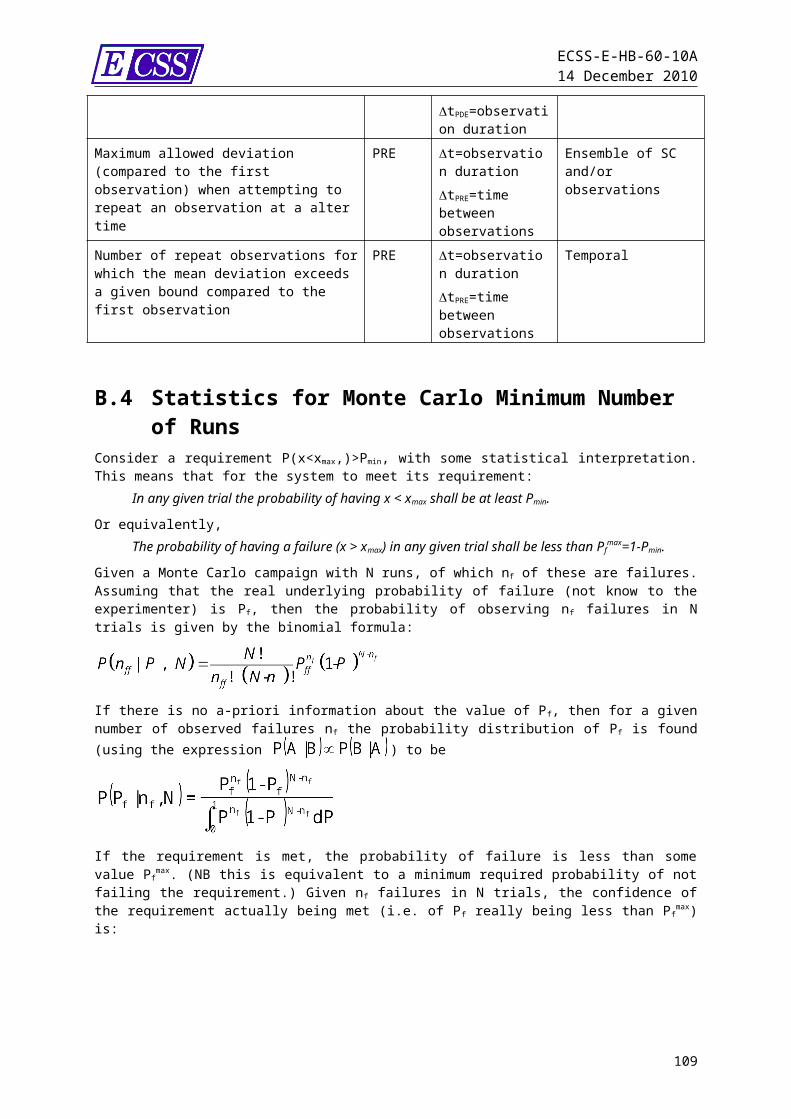
ECSS-E-HB-60-10A14 December 2010
o Frequency domain: The mean value of (t) (denoted M()) is equal to the transfer function gain |H(s)| at s=0 frequency (also called the static gain of the transfer function) times the mean value of e(t) (denoted M(e)):
M() = |H(0)| M(e)The PSD (Power Spectral Density) of (t) (denoted PSD(,f) with f the frequency) is equal to the square of the transfer function gain times the error source PSD (denoted PSD(e,f)):
PSD(,f) = |H(f)|2 PSD(e,f)
NOTE In case of uniform random noise, the PSD can be replaced by the noise variance. In other cases, the variance of the performance error is obtained by integration of the PSD over the suitable frequency band.
Step C.6.2.3c: Application of the error index to the performance errorLet us now assume that the performance error (t) has been computed accordingly to the previous rules, and its statistical characteristics are known (mean, covariance matrix and PSD for noises, maximum value for harmonics)
All indices: to apply indices to the performance error, one simply applies its temporal definition on the temporal performance error (t). For example, APE is defined as the instantaneous value of the performance error. Then the instantaneous value of (t) gives the APE. PSE special case: for a requirement on PSE over a time interval DT, the temporal definition APE((t))-APE((t-dt)) for any dt in ]0;DT] can lead to a high volume of calculations: indeed, it implies the computation of the APE difference over a sliding window of DT seconds. For one single harmonic error source, a frequency domain approximation can be used. Let us assume that (t) = A sin(2ft). Then it can be shown that:
o If f>1/2DT, then the maximum absolute value of the PSE over DT is 2A. o If f1/2DT, then the maximum absolute value of the PSE over DT is 2Asin(fDT).o An approximate formula can also be useful:
o If f>1/DT, then the maximum absolute value of the PSE over DT is 2A. o If f1/DT, then the maximum absolute value of the PSE over DT is 2AfDT.
NOTE 1 The approximate formula allows to cope with the frequency uncertainty of the performance error: the 2A maximum value is found for sine half period strictly smaller than DT.NOTE 2 The PSE requirements of our satellite example for one single sine error source can be illustrated in the frequency domain as shown on Figure C-1. The slope in low frequency domain means that the stability requirement is equivalent to some velocity limitation, whereas in high frequency domain, it is equivalent to angular position constraint.NOTE 3 The frequency computation rules can also be used by analogy with noise error source (considering for example the 6 value instead of 2A) or for several
109
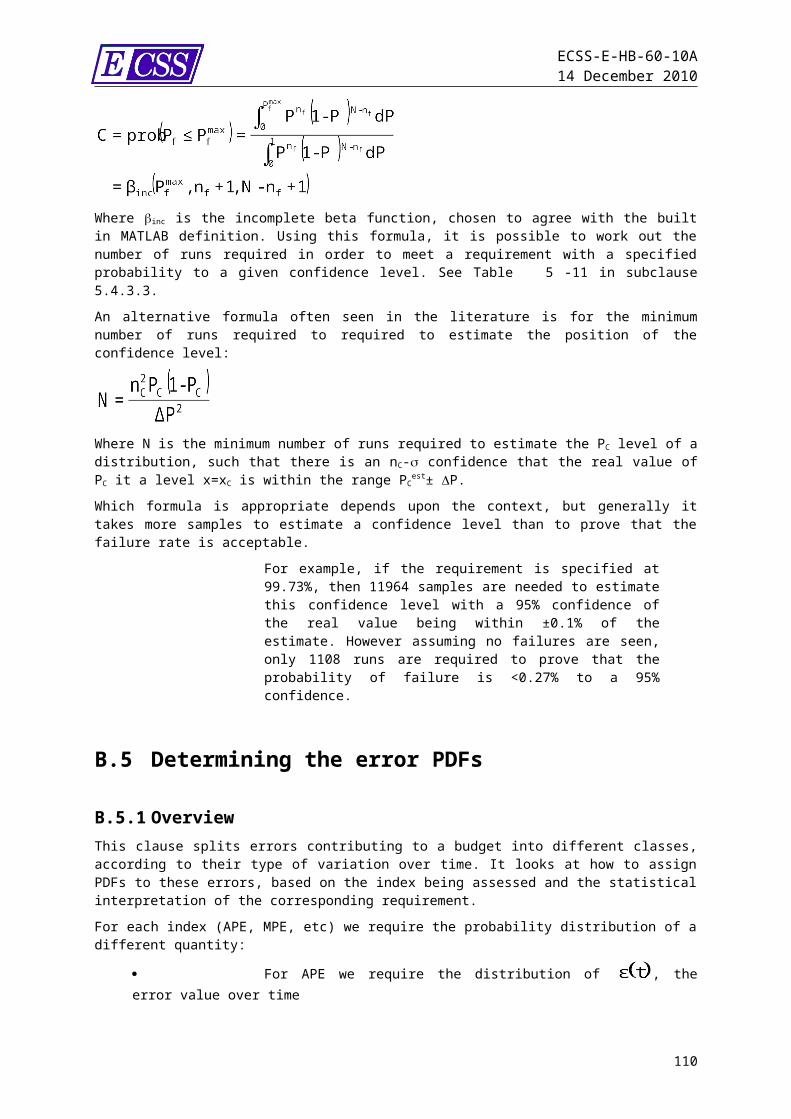
ECSS-E-HB-60-10A14 December 2010
harmonic sources with performance allocations. See clause C.7 for an example.NOTE 4 With these rules, it can be noticed that if DT tends to the observation period, then the stability contribution is equal to twice the APE contribution (peak-to-peak value for PSE instead of 0-peak value for APE).
Figure C-1: Frequency template of pointing and stability specifications for SPOT at AOCS level
C.6.2.4 Computation of total error and comparison to requirementAccording to clause 5, first a summation is computed inside each error class, and then the total error is computed as the sum of each class error. a. the mean and standard deviation of the total errors in each of the classes are
computed using the following method:1. If it can be shown that the errors are not correlated, then the following
summation rules apply:
2. If it can be shown that the errors are correlated, or if there is reason to suppose that they can be correlated, then the following (more conservative) summation rules are applied
Where means that the summation is over all errors grouped in this class
b. To find the mean and standard deviation of the total error, the means and standard deviations are summed as follows:
NOTE In some cases, the bias contribution is not summed with other classes and presented apart. Then we have a bias budget and a budget excluding bias.
Finally, the total error (generally the or 3 value) is compared to the maximum index value of the requirement. The requirement is met if the or 3 value is less that Imax with some margin.
C.6.3 Assessing compliance to control loop requirements C.3bbb1 and C.3bbb2
A practical way of assessing compliance to requirements on the stability margins, such as requirements (5) and (6) of our example, is to illustrate them on Black-Nichols diagrams, depending on satellite dispersions. Figure C-6 shows an example of such a diagram for 400 models with flexible mode frequency variation. On this example, the low frequency stability margins are not degraded by the flexible mode uncertainty.
110
Location (pointing)
Lines distortion (pointing and stability)
Ground sampling resolution variation + payload transfer function
Fl = 1/DTl
AAOCS_1
AAOCS_4
AOCS bandwidth Mechanical design such that disturbances < requirements
Log(f)
AAOCS_3
Fs=1/DTs
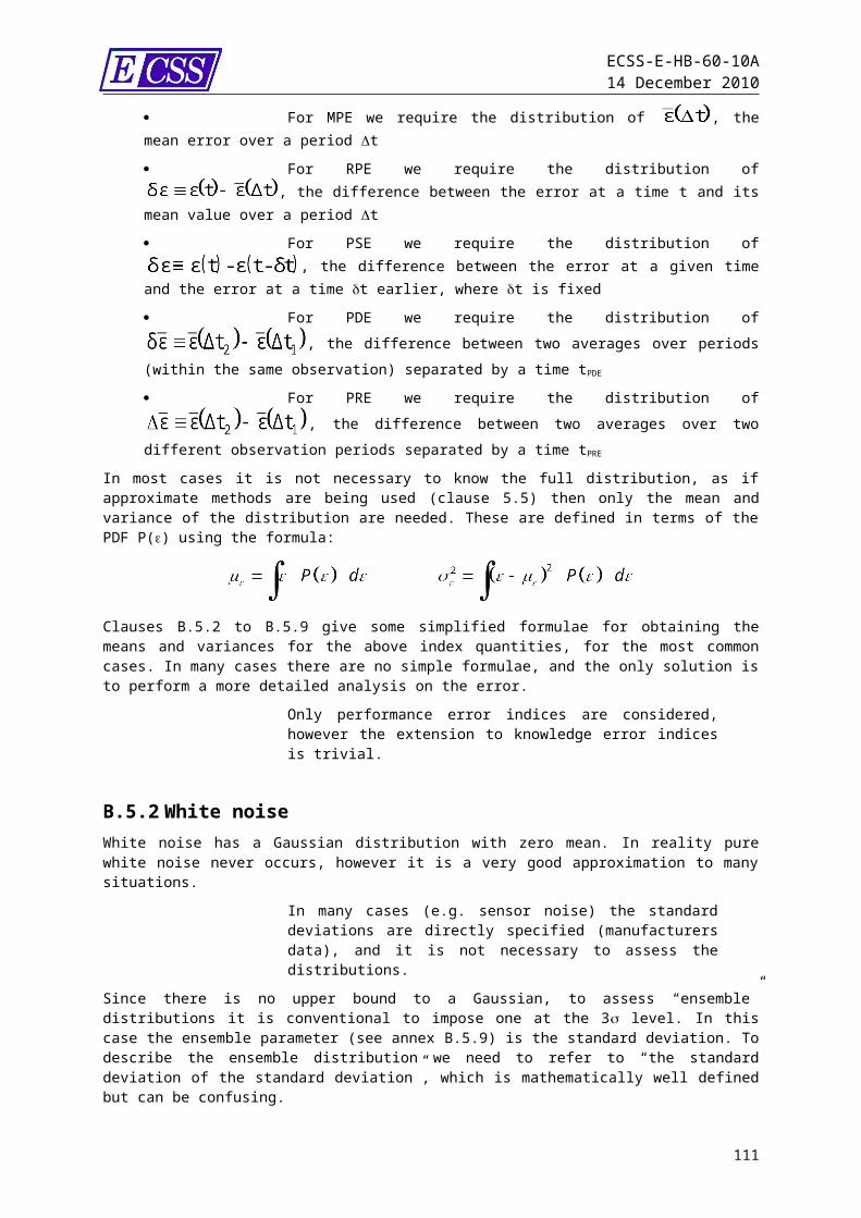
ECSS-E-HB-60-10A14 December 2010
Figure C-1: Black-Nichols diagram for flexible mode frequency uncertainty
The number of uncertain models to be used is similar to the number of simulations in a Monte Carlo campaign.
C.7 Performance budget examples
C.7.1 OverviewThis clause C.7 illustrates the computation of the performance budgets for temporal requirements C.3aaa1 to C.3aaa4 .
C.7.2 Pointing Knowledge Budget
C.7.2.1 GeneralWe begin with the knowledge budget because it is also part of the pointing budget. The requirement to be met is:
“The absolute value of the AKE of Euler angle between satellite frame and reference frame on each axis shall be less than 0.005 deg for 99.7% of time and 99.7% of satellite dispersions (modified mixed interpretation).”
Prob ( |AKE((t))|) < 0.005° ) > 0.997
111
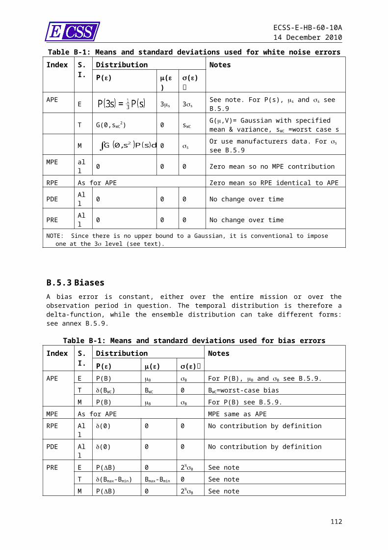
ECSS-E-HB-60-10A14 December 2010
NOTE The requirement specifies a condition to be met for 99.7% of satellite dispersions, which means that the budget computation should be done several times to cover the dispersions (each dispersion produces a different transfer function). For sake of simplicity, it is considered that the transfer functions correspond to worst case of satellite dispersions regarding the performance, and thus that if the budget meets the condition specified by the requirement, it is met for 99.7% of satellite dispersions.
C.7.2.2 Error sources identificationThe knowledge error sources are only the sensors measurement errors, that is, in our case, the star tracker errors (see ECSS-E-60-20 “Stars sensors terminology and performance specification”) and the gyro errors. Both measurements are processed through an estimation filter to compute the attitude, velocity and gyro drift estimation. Requirement C.3aaa2 applies to the attitude estimation output.Using groups defined in Table C-3, the sources are identified on Table C-1:
Table C-1: Pointing knowledge error sources Error source Error
group Star tracker internal error:
Distortion residue for each starResidual scale factor for each starStar catalogue errorsResidual thermal driftResidual relativistic aberration correction
Calibration errorMechanical error (ageing, launch)
Noise Equivalent Angle
STR measurement loss
HHHHH
BB
WN
T
Gyro error: Drift Calibration residueScale factor ARWRRW
BBWNWN
Gyro-STR Misalignment gyro-STRThermoelastic gyro-STR
BH
C.7.2.3 Computation of error sources contributionsThe transfer functions of interest are those between the gyro measurement and the attitude estimate, and between the star tracker measurement and the attitude estimate. Using a constant gain estimation filter, the transfer functions are illustrated on FigureC-1.
112

ECSS-E-HB-60-10A14 December 2010
Figure C-1: Estimation filter asymptotic transfer functions (Bode gain diagram)
Then the statistical characteristics of the performance error signal (the estimated attitude) (max amplitude, 3 value) are given on Table C-1.
Table C-1: Estimated attitude characteristics Error source Error
group
Source characteristics
Performance error characteristics
Star tracker internal error:Distortion residue for each starResidual scale factor for each starStar catalogue errorsResidual thermal driftResidual relativistic aberration correction
Calibration errorMechanical error (ageing, launch)
Noise Equivalent Angle
STR measurement loss
HHHHH
BB
WN
T
A1, f1
A2, f1
A3, f3
A4, f4
A5, f5
C1
C2
NEA, NEA, PSDNEA(f)
Simulation, T1
B1=|HSST(f1)|A1
B2=|HSST(f1)|A2
B3=|HSST(f3)|A3
B4=|HSST(f4)|A4
B5=|HSST(f5)|A5
D1=|HSST(0)|C1
D2=|HSST(0)|C2
1=|HSST(0)|NEA
PSD1(f) =|HSST(f)|².PSDNEA(f)
simulation, U1
Gyro error: Drift Calibration residueScale factor ARW
RRW
BBWN
WN
C3
C4
ARW, ARW, PSD ARW (f)
RRW, RRW, PSD RRW (f)
D3=|Hgyro(0)/s|C3
D4=|Hgyro(0)/s|C4
2=|HSST(0)|ARW
PSD2(f) =|Hgyro(f)|².PSDARW(f)
3=|HSST(0)|RRW
PSD3(f) =|HSST(f)|².PSDRRW(f)
113
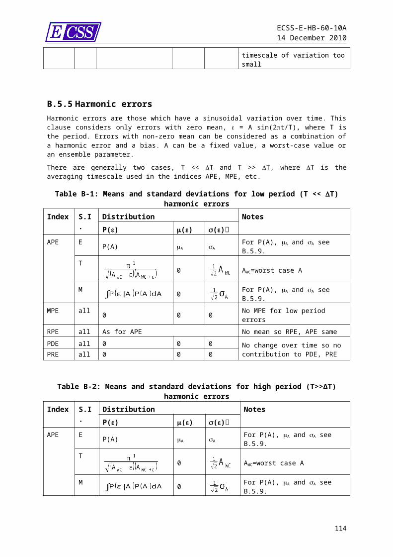
ECSS-E-HB-60-10A14 December 2010
Error source Error group
Source characteristics
Performance error characteristics
Misalignment gyro-STR
Thermoelastic gyro-STR
B
H
C5
A6, f6
D5=|H(0)|C5, with HSST or Hgyro depending on the reference frameB6=|H(f6)|A6, with HSST or Hgyro depending on the reference frame
Finally AKE index is applied to the estimated attitude: AKE is the instantaneous value of the estimated attitude.
C.7.2.4 Total error computation The AKE budget is given on Table C-1.
Table C-1: AKE budgetContribution class Summation rule
HarmonicH = B1+ B2 +
B1 and B2 at correlated (same frequency), the others are not. White Noise = , = 1+ 2+ 3
BiasB =
Transient U1 (for example similar to standard deviation)Total error total = (1)
total = µ + B(1) The harmonic contribution is taken as standard deviation (thus divided by 2 ½) to be consistent
with noise standard deviation
Finally, the requirement in C.7.2.1 is met if µtotal+3total < 0.005 deg.
C.7.3 Pointing budget
C.7.3.1 GeneralFor pointing performance, the requirement to be met is:“The absolute value of the APE of Euler angle between satellite frame and reference frame on each axis shall be less than 0.05 deg for 99.7% of time and 99.7% of satellite dispersions” (modified mixed interpretation).Prob ( |APE((t))|) < 0.05° ) > 0.997
NOTE For sake of simplicity, worst case of satellite dispersions is considered.
114
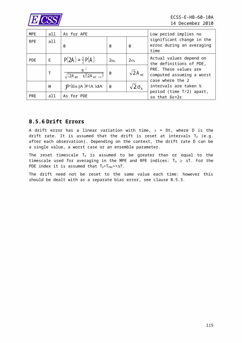
ECSS-E-HB-60-10A14 December 2010
C.7.3.2 Identification of error sourcesAccording to groups defined in clause 5, the error sources for pointing budget are given on Table C-1.
Table C-1: Pointing error sourcesError sources Error groupGyro-stellar errors (see AKE budget)
H, T, WN, B
Control errors (in closed-loop control bandwidth)Environmental disturbances residue (solar pressure, drag, gravity gradient, magnetic torque, etc.)
B, H (not at the same frequency)
Actuator errors
Reaction wheelsStiction (0 rpm crossing)NoiseMicrovibrationsMisalignments
Magneto-Torquer BarsOFF/ON, modulation
TWNHB
T, HMechanismsSteerable mirror biasSolar array drive motor (SADM)
BH
C.7.3.3 Computation of error sources contributionsAccording to the six error sources locations, six transfer functions between the error sources and the performance error (the satellite real attitude) are considered:a. Transfer function between gyro-stellar estimation and attitude: Hest, of low-pass
filter typeb. Transfer function between actuators and attitude: HRWS and HMTB, of low-pass or
band-pass filter typec. Transfer function between external torques and attitude: Hext, of low-pass or
band-pass filterd. Transfer function between payload disturbances and attitude: HPLD
e. Transfer function between SADM and attitude: HSADM
The computation of the performance signal characteristics is similar to the one applied for knowledge requirement, taking the error classes into account. Finally, APE index is applied to attitude contributions: APE is the instantaneous value of attitude.
115
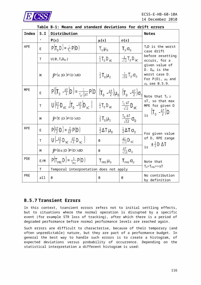
ECSS-E-HB-60-10A14 December 2010
C.7.3.4 Total error computationOnce having each contribution from each error source, summations rules inside classes apply, and then the total error is computed by summing classes errors. Finally, the requirement is met if µtotal+3total < 0.05 deg.
C.7.4 Pointing stability Budget (Requirements C.3aaa3 and C.3aaa4)
C.7.4.1 GeneralFor stability performance, two requirements are imposed:
For long term stability:“The absolute value of the PSE over 10s of Euler angle between satellite frame and reference frame on each axis shall be less than 0.005 deg for 99.7% of time and 99.7% of satellite dispersions” (modified mixed interpretation).Prob ( |PSE((t,dt))|) < 0.005° ) > 0.997, 0<dt10s For short term stability:“The absolute value of the PSE over 10ms of Euler angle between satellite frame and reference frame on each axis shall be less than 5.10-5deg for 99.7% of time and 99.7% of satellite dispersions” (modified mixed interpretation).Prob ( |PSE((t,dt))|) < 5.10-5°) > 0.997, 0<dt10ms
C.7.4.2 Identification of error sourcesThe stability error sources are identical to those of pointing, except for bias type ones, that have no contribution on the budget.
C.7.4.3 Computation of error sources contributionsThe transfer functions are the same as for the pointing requirement, and the characteristics of the performance error signal (real attitude of the satellite) are the same.The difficulty lies in the computation of the PSE index, which is defined as APE(t)-APE(t-dt). The requirement is not met unless dt is in the range between 0 and DT = 10s or 10 ms.In this clause, the frequency template for sine errors and white noise error is applied. Let us choose three errors among the error sources:
An environmental disturbance torque at orbital frequency 0 = 0.001 rad/s whose effect on the attitude is a sine error 1(t)=A1.sin(0t) with A1=0.005 deg. A reaction wheel microvibration at f=40 Hz whose effect on the attitude is a sine error 2(t)=A2.sin(ft), with A2 = 0.001 deg. The star tracker noise equivalent angle whose effect on the attitude 3(t) is a noise with mean µ and standard deviation , and PSD P(f) for example illustrated on Figure C-1. FAOCS denotes the AOCS bandwidth, fest is the estimation filter cut-off frequency, and fe is the star tracker sampling frequency.
116
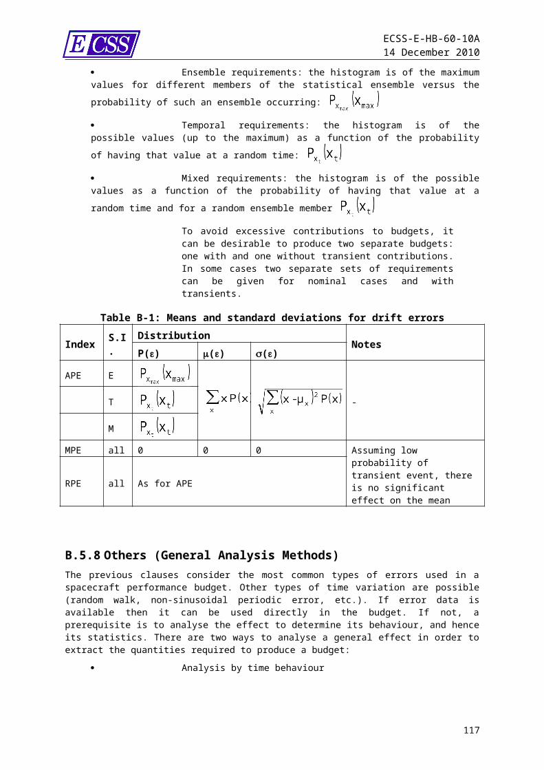
ECSS-E-HB-60-10A14 December 2010
Figure C-1: Attitude PSD template due to star tracker noiseLet us first compute the harmonic contribution to the budget.The sine frequency templates which represent the maximum amplitude of the harmonic performance error meeting the stability requirements are shown on Figure C-2. They have been computed using the approximate formula.
Figure C-2: Frequency stability templates for requirements C.3aaa3 and C.3aaa4
Using these templates, it can be easily checked that 1(t) and 2(t) taken separately meet requirement for long term stability, but 2(t) is too large for requirement on short term stability (dotted line). It is important to compute the PSE contributions in order to be sure that requirement on long term stability is met taken simultaneously 1(t) and 2(t).
117
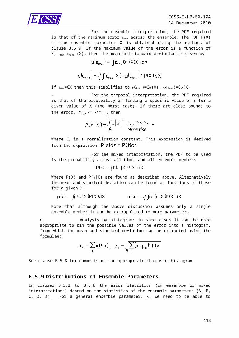
ECSS-E-HB-60-10A14 December 2010
For long term stability, the separation frequency is fs = 1/DT = 0.03 Hz. Then, 1(t) frequency f1 is lower and 2(t) frequency f2 is higher. According to the approximate formula, one gets:
Max (|PSE(1(t))|) = B1 = 20.005f1DT = 5.10-5 deg Max (|PSE(2(t))|) = B2 = 20.001 = 0.002 deg
It can be noticed that in this case, 1(t) which is of higher amplitude than 2(t) contributes much less than 2(t) to the stability budget.Let us now apply the same type of computation to noise error for long term stability requirement. The rules are the following:
For f<fs, the PSE index is redefined as (APE(3(t)-APE(3(t-dt))DT, where 3(t) is the angular velocity (in our case, it is considered that 3(t) is the time derivative of 3(t)). For f>fs, standard PSE definition applies.
Then the standard deviation of the PSE can be decomposed into the quadratic sum of two terms, one for low frequencies L, one for high frequencies H, defined as follows:
NOTE With these rules, it can verified that if fs=0 (stability over the observation period), then the standard deviation of PSE equals the standard deviation of APE.
C.7.4.4 Total error computationThe total error computation is similar to APE index, except that no bias contributes to PSE. According to the three error sources, the error combination is as described on Table C-1.
Table C-1: PSE contributions summationError class Error contributionHarmonic H =
Noise =
Total error
NOTE: Because the stability requirements are expressed as a peak-to-peak value, one can choose n = 6 (twice the 3 value)
118


![Pointing Error Engineering Tool - European Space Agencypeet.estec.esa.int/files/ASTOS-PEET-TN-001_Iss1.3...[AD3] ECSS-E-HB-60-10A; Space Engineering, Control Performance Guidelines](https://img.pdfslide.net/doc/110x75/612e87091ecc51586942dec0/pointing-error-engineering-tool-european-space-ad3-ecss-e-hb-60-10a-space.jpg)