ECTURE Communication Networks: Sharing and …web.mit.edu/6.02/www/s2010/handouts/lectures/L15-notes.pdf · communication networks: sharing and switches bit rate,5 of a link connected

MIT 6.02 Lecture NotesSpring 2010 (Last update: March 25, 2010)Comments, questions or bug reports?

Please contact [email protected]

LECTURE 15Communication Networks: Sharing

and Switches

So far in this course we have studied techniques to engineer a point-to-point communicationlink. Two important considerations were at the heart of most everything we studied:

1. Improving link communication reliability: Inter-symbol interference (ISI) and noise con-spired to introduce errors in transmission. We developed techniques to select a suit-able sampling rate and method using eye diagrams and then reduced the bit-error rateusing channel coding (block, Reed-Solomon, and convolutional codes).

2. Sharing a link: We wanted to share the same communication medium amongst kdifferent receivers, each tuned to a different frequency. To achieve this goal, we useddigital modulation, and learned that understanding the frequency response of an LTIsystem and designing filters are key building blocks for this task.

We now turn to the study of communication networks—systems that connect three ormore computers (or phones)1 together.

The key idea that we will use to engineer communication networks is composition: wewill build small networks by composing links together, and build larger networks by com-posing smaller networks together.

The fundamental challenges in the design of a communication network are the sameas those that face the designer of a communication link: sharing and reliability. The bigdifference is that the sharing problem is considerably more challenging, and many morethings can go wrong in networking2 many computers together, making communicationmore unreliable than a single link’s unreliability. The next few lectures will show you thesechallenges and you will understand the key ideas in how these challenges are overcome.

In addition to sharing and reliability, an important and difficult problem that manycommunication networks (such as the Internet) face is scalability: how to engineer a verylarge, global system. We won’t say very much about scalability in this course, leaving thisimportant issue to future courses in EECS.

1The distinction between a phone and a computer is rapidly vanishing, so the difference is rather artificial.2As one wag put it: “Networking, just one letter away from not working.”

1

2 LECTURE 15. COMMUNICATION NETWORKS: SHARING AND SWITCHES

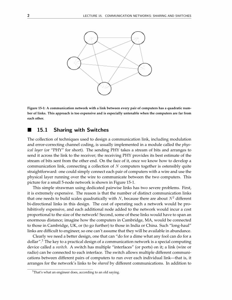
Figure 15-1: A communication network with a link between every pair of computers has a quadratic num-ber of links. This approach is too expensive and is especially untenable when the computers are far fromeach other.

� 15.1 Sharing with Switches

The collection of techniques used to design a communication link, including modulationand error-correcting channel coding, is usually implemented in a module called the phys-ical layer (or “PHY” for short). The sending PHY takes a stream of bits and arranges tosend it across the link to the receiver; the receiving PHY provides its best estimate of thestream of bits sent from the other end. On the face of it, once we know how to develop acommunication link, connecting a collection of N computers together is ostensibly quitestraightforward: one could simply connect each pair of computers with a wire and use thephysical layer running over the wire to communicate between the two computers. Thispicture for a small 5-node network is shown in Figure 15-1.

This simple strawman using dedicated pairwise links has two severe problems. First,it is extremely expensive. The reason is that the number of distinct communication linksthat one needs to build scales quadratically with N , because there are about N2 differentbi-directional links in this design. The cost of operating such a network would be pro-hibitively expensive, and each additional node added to the network would incur a costproportional to the size of the network! Second, some of these links would have to span anenormous distance; imagine how the computers in Cambridge, MA, would be connectedto those in Cambridge, UK, or (to go further) to those in India or China. Such “long-haul”links are difficult to engineer, so one can’t assume that they will be available in abundance.

Clearly we need a better design, one that can “do for a dime what any fool can do for adollar”.3 The key to a practical design of a communication network is a special computingdevice called a switch. A switch has multiple “interfaces” (or ports) on it; a link (wire orradio) can be connected to each interface. The switch allows multiple different communi-cations between different pairs of computers to run over each individual link—that is, itarranges for the network’s links to be shared by different communications. In addition to

3That’s what an engineer does, according to an old saying.

SECTION 15.1. SHARING WITH SWITCHES 3

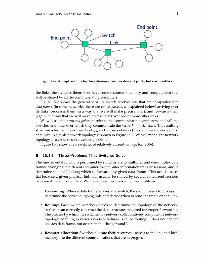
Figure 15-2: A simple network topology showing communicating end points, links, and switches.

the links, the switches themselves have some resources (memory and computation) thatwill be shared by all the communicating computers.

Figure 15-2 shows the general idea. A switch receives bits that are encapsulated indata frames (in some networks, these are called packets, as explained below) arriving overits links, processes them (in a way that we will make precise later), and forwards them(again, in a way that we will make precise later) over one or more other links.

We will use the term end points to refer to the communicating computers, and call theswitches and links over which they communicate the network infrastructure. The resultingstructure is termed the network topology, and consists of nodes (the switches and end points)and links. A simple network topology is shown in Figure 15-2. We will model the networktopology as a graph to solve various problems.

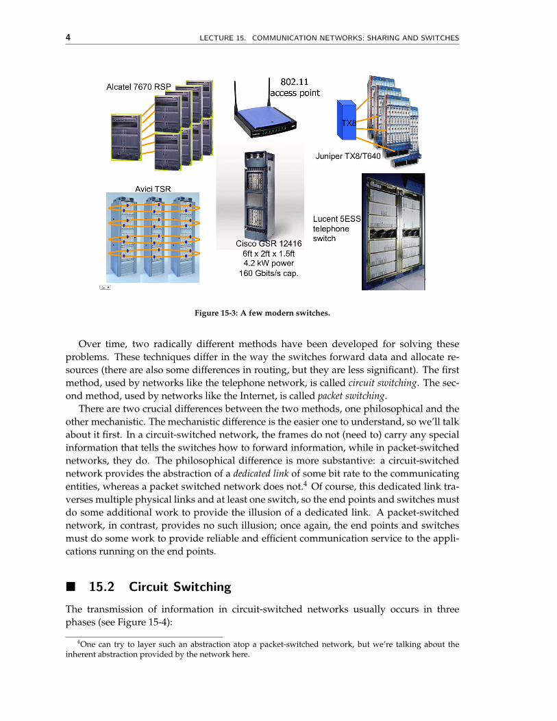
Figure 15-3 show a few switches of relatively current vintage (ca. 2006).

� 15.1.1 Three Problems That Switches Solve

The fundamental functions performed by switches are to multiplex and demultiplex dataframes belonging to different computer-to-computer information transfer sessions, and todetermine the link(s) along which to forward any given data frame. This task is essen-tial because a given physical link will usually be shared by several concurrent sessionsbetween different computers. We break these functions into three problems:

1. Forwarding: When a data frame arrives at a switch, the switch needs to process it,determine the correct outgoing link, and decide when to send the frame on that link.

2. Routing: Each switch somehow needs to determine the topology of the network,so that it can correctly construct the data structures required for proper forwarding.The process by which the switches in a network collaboratively compute the networktopology, adapting to various kinds of failures, is called routing. It does not happenon each data frame, but occurs in the “background”.

3. Resource allocation: Switches allocate their resources—access to the link and localmemory—to the different communications that are in progress.


Figure 15-3: A few modern switches.

Over time, two radically different methods have been developed for solving theseproblems. These techniques differ in the way the switches forward data and allocate re-sources (there are also some differences in routing, but they are less significant). The firstmethod, used by networks like the telephone network, is called circuit switching. The sec-ond method, used by networks like the Internet, is called packet switching.

There are two crucial differences between the two methods, one philosophical and theother mechanistic. The mechanistic difference is the easier one to understand, so we’ll talkabout it first. In a circuit-switched network, the frames do not (need to) carry any specialinformation that tells the switches how to forward information, while in packet-switchednetworks, they do. The philosophical difference is more substantive: a circuit-switchednetwork provides the abstraction of a dedicated link of some bit rate to the communicatingentities, whereas a packet switched network does not.4 Of course, this dedicated link tra-verses multiple physical links and at least one switch, so the end points and switches mustdo some additional work to provide the illusion of a dedicated link. A packet-switchednetwork, in contrast, provides no such illusion; once again, the end points and switchesmust do some work to provide reliable and efficient communication service to the appli-cations running on the end points.

� 15.2 Circuit Switching

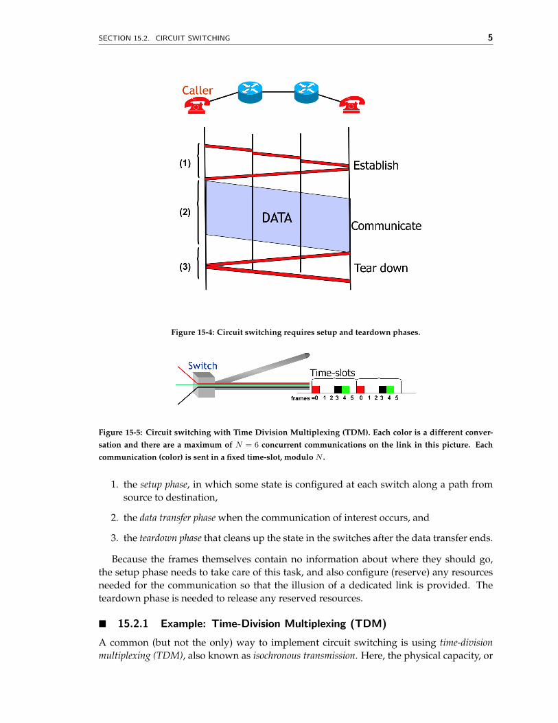
The transmission of information in circuit-switched networks usually occurs in threephases (see Figure 15-4):

4One can try to layer such an abstraction atop a packet-switched network, but we’re talking about theinherent abstraction provided by the network here.

SECTION 15.2. CIRCUIT SWITCHING 5

Figure 15-4: Circuit switching requires setup and teardown phases.

Figure 15-5: Circuit switching with Time Division Multiplexing (TDM). Each color is a different conver-sation and there are a maximum of N = 6 concurrent communications on the link in this picture. Eachcommunication (color) is sent in a fixed time-slot, modulo N .

1. the setup phase, in which some state is configured at each switch along a path fromsource to destination,

2. the data transfer phase when the communication of interest occurs, and

3. the teardown phase that cleans up the state in the switches after the data transfer ends.

Because the frames themselves contain no information about where they should go,the setup phase needs to take care of this task, and also configure (reserve) any resourcesneeded for the communication so that the illusion of a dedicated link is provided. Theteardown phase is needed to release any reserved resources.

� 15.2.1 Example: Time-Division Multiplexing (TDM)

A common (but not the only) way to implement circuit switching is using time-divisionmultiplexing (TDM), also known as isochronous transmission. Here, the physical capacity, or


bit rate,5 of a link connected to a switch, C (in bits/s), is conceptually broken into somenumber N of virtual “channels” (or time slots), such that the ratio C/N bits/s is sufficientfor each information transfer session (such as a telephone call between two parties). Callthis ratio, R, the rate of each independent transfer session. Now, if we constrain each frameto be of some fixed size, s bits, then the switch can perform time multiplexing by allocatingthe link’s capacity in time-slots of length s/C units each, and by associating the ith time-slice to the ith transfer (modulo N ). It is easy to see that this approach provides eachsession with the required rate of R bits/s, because each session gets to send s bits over atime period of Ns/C seconds, and the ratio of the two is equal to C/N = R bits/s.

Each data frame is therefore forwarded by simply using the time slot in which it arrivesat the switch to decide which port it should be sent on. Thus, the state set up during thefirst phase has to associate one of these channels with the corresponding soon-to-followdata transfer by allocating the ith time-slice to the ith transfer. The end points transmittingdata send frames only at the specific time-slots that they have been told to do so by thesetup phase.

Other ways of doing circuit switching include wavelength division multiplexing (WDM),frequency division multiplexing (FDM), and code division multiplexing (CDM); the latter two(as well as TDM) are used in some wireless networks, while WDM is used in some high-speed optical networks.

� 15.2.2 Pros and Cons

Circuit switching makes sense for a network where the workload is relatively uniform,with all information transfers using the same capacity, and where each transfer uses a con-stant bit rate (or near-constant bit rate). The most compelling example of such a workloadis telephony, where each digitized voice call might operate at 64 kbits/s. Switching wasfirst invented for the telephone network, well before computers were on the scene, so thisdesign choice makes a great deal of sense. The classical telephone network as well as thecellular telephone network in most countries still operate in this way, though telephonyover the Internet is becoming increasingly popular and some of the network infrastructureof the classical telephone networks is moving toward packet switching.

However, circuit-switching tends to waste link capacity if the workload has a variablebit rate, or if the frames arrive in bursts at a switch. Because a large number of computerapplications induce burst data patterns, we should consider a different link sharing strat-egy for computer networks. Another drawback of circuit switching shows up when the(N + 1)st communication arrives at a switch whose relevant link already has the maxi-mum number (N ) of communications going over it. This communication must be denied

5This number is sometimes referred to as the “bandwidth” of the link. Technically, bandwidth is a quantitymeasured in Hertz and refers to the width of the frequency over which the transmission is being done. Toavoid confusion, we will use the term “bit rate” to refer to the number of bits per second that a link is currentlyoperating at, but the reader should realize that the literature often uses “bandwidth” to refer to this term. Thereader should also be warned that some people (curmudgeons?) become apoplectic when they hear someoneusing “bandwidth” for the bit rate of a link. A more reasonable position is to realize that when the context isclear, there’s not much harm in using “bandwidth”. The reader should also realize that in practice most wiredlinks usually operate at a single bit rate (or perhaps pick one from a fixed set when the link is configured),but that wireless links using radio communication can operate at a range of bit rates, adaptively selecting themodulation and coding being used to cope with the time-varying channel conditions caused by interferenceand movement.

SECTION 15.3. PACKET SWITCHING 7

access (or admission) to the system, because there is no capacity left for it. For applicationsthat require a certain minimum bit rate, this approach might make sense, but even in thatcase a “busy tone” is the result. However, there are many applications that don’t have aminimum bit rate requirement (email and file downloads are examples); for this reason aswell, a different sharing strategy is worth considering.

Packet switching doesn’t have these drawbacks.

� 15.3 Packet Switching

The best way to overcome the above inefficiencies is to allow for any sender to transmitdata at any time, but yet allow the link to be shared. Packet switching is a way to accom-plish this task, and uses a tantalizingly simple idea: add to each frame of data a little bit ofinformation that tells the switch how to forward it. This information is added in the formof a packet header and the resulting frame is called a packet.6 In the most common form ofpacket switching, the header of each packet contains the address of the destination, whichuniquely identifies the destination of data. The switches use this information to processand forward each packet. Packets usually also include the sender’s address to help thereceiver send messages back to the sender.

The job of the switch is to use the destination address as a key and perform a lookup ona data structure called a routing table (or forwarding table; the distinction between the twois sometimes important and will become apparent in a later lecture in the course). Thislookup returns an outgoing link to forward the packet on its way toward the intendeddestination.

While forwarding is a relatively simple lookup in a data structure, the trickier questionthat we will spend time on is determining how the entries in the routing table are ob-tained. The plan is to use a background process called a routing protocol, which is typicallyimplemented in a distributed manner by the switches. There are several types of routingprotocols that one might consider, and we will study two common classes of protocols inlater lectures. For now, it is enough to understand that the result of running a routing pro-tocol is to obtain routes (which you can think of as paths for the time being) in the networkto every destination—each switch dynamically constructs and updates its routing tableusing the routing protocol and uses this table to forward data packets.

Switches in packet-switched networks that implement the functions described in thissection are often called routers. Packet forwarding and routing using the Internet Protocol(IP) in the Internet is an example of packet-switching.

� 15.3.1 Why Packet Switching Works: Statistical Multiplexing

Packet switching does not provide the illusion of a dedicated link to any pair of commu-nicating end points, but it has a few things going for it:

1. it doesn’t waste the capacity of any link because each switch can send any packetavailable to it that needs to use that link,

2. it does not require any setup or teardown phases and so can be used even for smalltransfers without any overhead, and

6Sometimes, the term datagram is used instead of (or in addition to) the term “packet”.


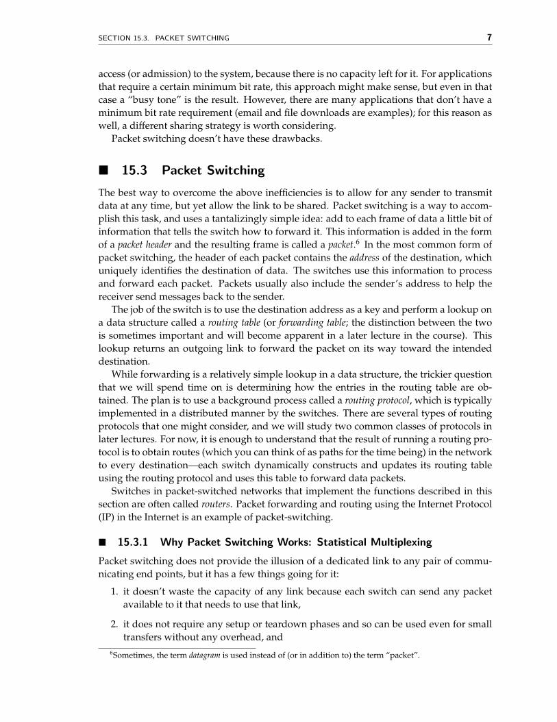
Figure 15-6: Packet switching works because of statistical multiplexing. This picture shows a simulationof N senders, each connected at a fixed bit rate of 1 megabit/s to a switch, sharing a single outgoing link.The y-axis shows the aggregate bit rate (in megabits/s) as a function of time (in milliseconds). In thissimulation, each sender is in either the “on” (sending) state or the “off” (idle) state; the durations of eachstate are drawn from a Pareto distribution (which has a “heavy tail”).

3. it can provide variable data rates to different communications essentially on an “asneeded” basis.

At the same time, notice that because there is no reservation of resources, packets couldarrive faster than can be sent over a link, and the switch must be able to handle suchsituations. Switches deal with transient bursts of traffic that arrive faster than a link’s bitrate using queues. We will spend some time understanding what a queue does and how itabsorbs bursts, but for now, let’s assume that a switch has large queues and understandwhy packet switching actually works.

Packet switching supports end points sending data at variable rates. If a large numberof end points conspired to send data in a synchronized way to exercise a link at the sametime, then one would end up having to provision a link to handle the peak synchronizedrate for packet switching to provide reasonable service to all the concurrent communica-tions.

Fortunately, at least in a network with benign, or even greedy individual communicat-ing pairs, it is highly unlikely that all the senders will be perfectly synchronized. Evenwhen senders send long bursts of traffic, as long as they alternate between “on” and “off”states and move between these states at random (the probability distributions for thesecould be complicated and involve “heavy tails” and high variances), the aggregate traffic

SECTION 15.3. PACKET SWITCHING 9

Figure 15-7: Network traffic variability.

of multiple senders tends to smooth out a bit.7

An example is shown in Figure 15-6. The x-axis is time in milliseconds and the y-axisshows the bit rate of the set of senders. Each sender has a link with a fixed bit rate connect-ing it to the switch. The picture shows how the aggregate bit rate over this short time-scale(4 seconds), though variable, becomes smoother as more senders share the link. This kindof multiplexing relies on the randomness inherent in the concurrent communications, andis called statistical multiplexing.

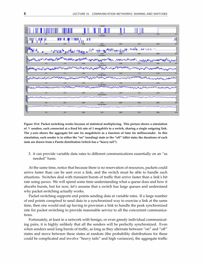
Real-world traffic has bigger bursts than shown in this picture and the data rate usu-ally varies by a large amount depending on time of day. Figure 15-7 shows the bit ratesobserved at an MIT lab for different network applications. Each point on the y-axis isa 5-minute average, so it doesn’t show the variations over smaller time-scales as in theprevious figure. However, it shows how much variation there is with time-of-day.

So far, we have discussed how the aggregation of multiple sources sending data tendsto smooth out traffic a bit, enabling the network designer to avoid provisioning a link forthe sum of the peak offered loads of the sources. In addition, for the packet switching ideato really work, one needs to appreciate the time-scales over which bursts of traffic occur inreal life.

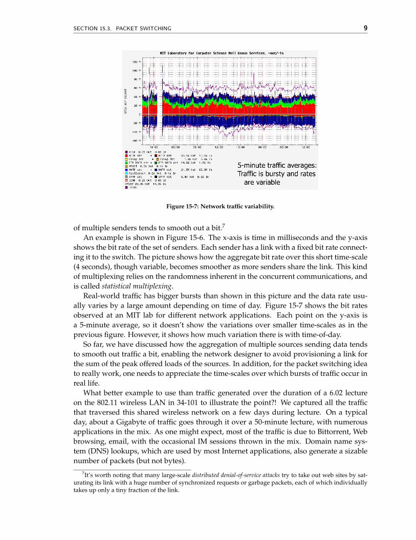
What better example to use than traffic generated over the duration of a 6.02 lectureon the 802.11 wireless LAN in 34-101 to illustrate the point?! We captured all the trafficthat traversed this shared wireless network on a few days during lecture. On a typicalday, about a Gigabyte of traffic goes through it over a 50-minute lecture, with numerousapplications in the mix. As one might expect, most of the traffic is due to Bittorrent, Webbrowsing, email, with the occasional IM sessions thrown in the mix. Domain name sys-tem (DNS) lookups, which are used by most Internet applications, also generate a sizablenumber of packets (but not bytes).

7It’s worth noting that many large-scale distributed denial-of-service attacks try to take out web sites by sat-urating its link with a huge number of synchronized requests or garbage packets, each of which individuallytakes up only a tiny fraction of the link.


1 second windows

100 ms windows

!"#$%&

'(&)*$&

!"#$%&

'(&)*$&

10 ms windows

Figure 15-8: Traffic bursts at different time-scales, showing some smoothing. Bursts still persist, though.

Figure 15-8 shows the aggregate amount of data, in bytes, as a function of time, overdifferent time durations. The top picture shows the data over 10 millisecond windows—here, each y-axis point is the total number of bytes observed over the wireless networkcorresponding to a non-overlapping 10-millisecond time window. We show the data herefor a randomly chosen time period that lasts 17 seconds. The most noteworthy aspect ofthis picture is the bursts that are evident: the maximum (not shown is as high as 50 Kbytesover this duration, but also note how successive time windows could change betweenclose to 20 Kbytes and nearly 0. From time to time, larger bursts occur where the networkis essentially continuously in use (for example, starting at 14:12:38.55).

The middle picture shows what happens when we look at 100 millisecond windows.Clearly, bursts persist, but the variance has reduced. When we move to 1 second windows,we see the same effect persisting, though again it’s worth noting that the bursts don’tactually disappear.

These data sets exemplify the traffic dynamics that a network designer has to planfor while designing a network. One could pick a data rate that is higher than the peakexpected over a short time-scale, but that would be several times larger than picking asmaller value and using a queue to absorb the bursts and send out packets over a link ofa smaller rate. In practice, this problem is complicated because network sources are not

SECTION 15.4. UNDERSTANDING NETWORK DELAYS 11

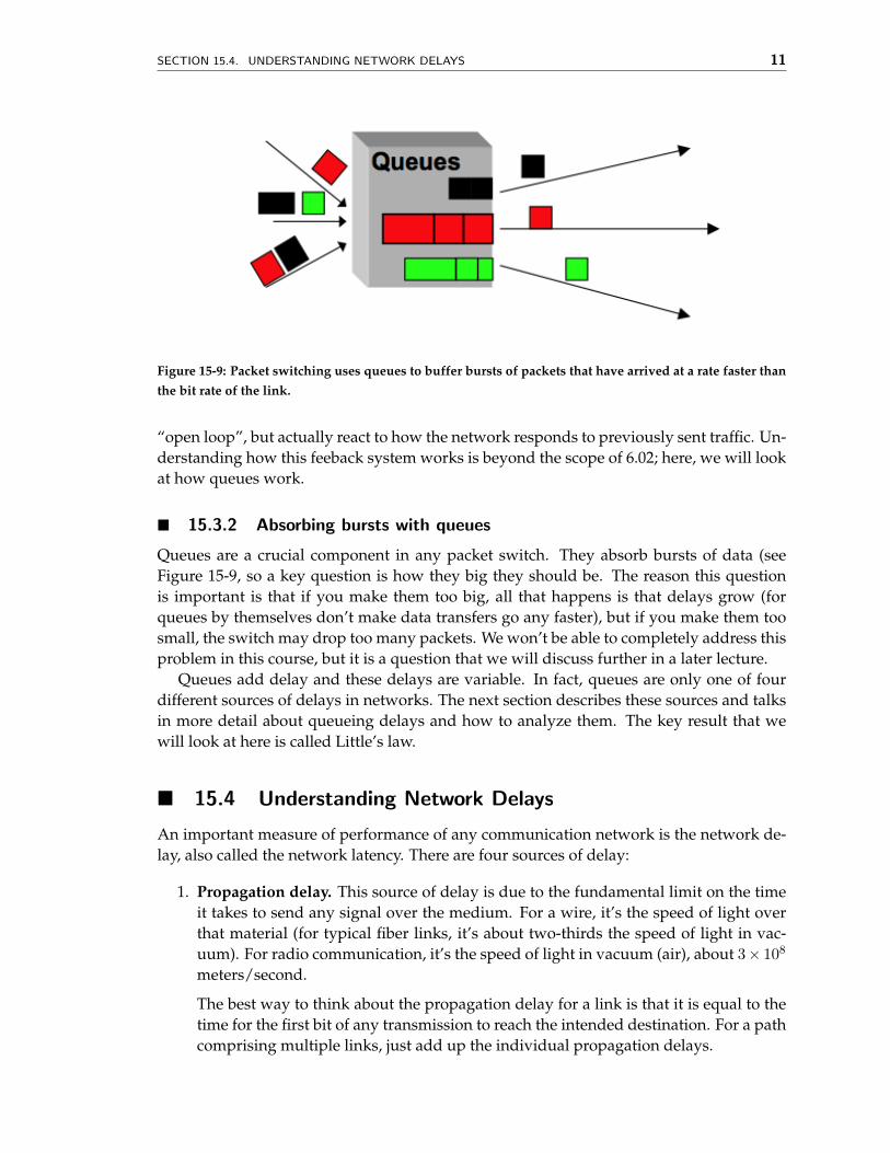
Figure 15-9: Packet switching uses queues to buffer bursts of packets that have arrived at a rate faster thanthe bit rate of the link.

“open loop”, but actually react to how the network responds to previously sent traffic. Un-derstanding how this feeback system works is beyond the scope of 6.02; here, we will lookat how queues work.

� 15.3.2 Absorbing bursts with queues

Queues are a crucial component in any packet switch. They absorb bursts of data (seeFigure 15-9, so a key question is how they big they should be. The reason this questionis important is that if you make them too big, all that happens is that delays grow (forqueues by themselves don’t make data transfers go any faster), but if you make them toosmall, the switch may drop too many packets. We won’t be able to completely address thisproblem in this course, but it is a question that we will discuss further in a later lecture.

Queues add delay and these delays are variable. In fact, queues are only one of fourdifferent sources of delays in networks. The next section describes these sources and talksin more detail about queueing delays and how to analyze them. The key result that wewill look at here is called Little’s law.

� 15.4 Understanding Network Delays

An important measure of performance of any communication network is the network de-lay, also called the network latency. There are four sources of delay:

1. Propagation delay. This source of delay is due to the fundamental limit on the timeit takes to send any signal over the medium. For a wire, it’s the speed of light overthat material (for typical fiber links, it’s about two-thirds the speed of light in vac-uum). For radio communication, it’s the speed of light in vacuum (air), about 3× 108

meters/second.

The best way to think about the propagation delay for a link is that it is equal to thetime for the first bit of any transmission to reach the intended destination. For a pathcomprising multiple links, just add up the individual propagation delays.


2. Processing delay. Whenever a packet (or data frame) enters a switch, it needs tobe processed before it is sent over the outgoing link. In a packet-switched network,this processing involves, at the least, looking up the header of the packet in a tableto determine the outgoing link. It may also involve operations like computing apacket checksum, modifying the packet’s header, etc. The total time taken for allsuch operations is called the processing delay of the switch.

3. Transmission delay. The transmission delay of a link is the time it takes for a packetof size S bits to traverse the link. If the bit rate of the link is R bits/second, then thetransmission delay is S/R seconds.

4. Queueing delay. Queues are a fundamental data structure used in packet-switchednetworks to absorb bursts of data arriving for an outgoing link at speeds that are(transiently) faster than the link’s bit rate. The time spent by a packet waiting in thequeue is its queueing delay.

Unlike the other components mentioned above, the queueing delay is usually vari-able. In many networks, it might also be the dominant source of delay, accounting forabout 50% (or more) of the delay experienced by packets when the network is con-gested. In some networks, such as those with satellite links, the propagation delaycould be the dominant source of delay.

� 15.4.1 Little’s Law

A common method used by engineers to analyze network performance, particularly delayand throughput (the rate at which packets are delivered), is queueing theory. In this course,we will use an important, widely applicable result from queueing theory, called Little’s law(or Little’s theorem).8 It’s used widely in the performance evaluation of systems rangingfrom communication networks to factory floors to manufacturing systems.

For any stable (i.e., where the queues aren’t growing without bound) queueing system,Little’s law relates the average arrival rate of items (e.g., packets), λ, the average delayexperienced by an item in the queue, D, and the average number of items in the queue, N .The formula is simple and intuitive:

N = λ×D (15.1)

Example. Suppose packets arrive at an average rate of 1000 packets per second intoa switch, and the rate of the outgoing link is larger than this number. (If the outgoingrate is smaller, then the queue will grow unbounded.) It doesn’t matter how inter-packetarrivals are distributed; packets could arrive in weird bursts according to complicateddistributions. Now, suppose there are 50 packets in the queue on average. That is, if wesample the queue size at random points in time and take the average, the number is 50packets.

Then, from Little’s law, we can conclude that the average queueing delay experiencedby a packet is 50/1000 seconds = 50 milliseconds.

8This “queueing formula” was first proved in a general setting by John D.C. Little, who is now an InstituteProfessor at MIT (he also received his PhD from MIT in 1955). In addition to the result that bears his name, heis a pioneer in marketing science.


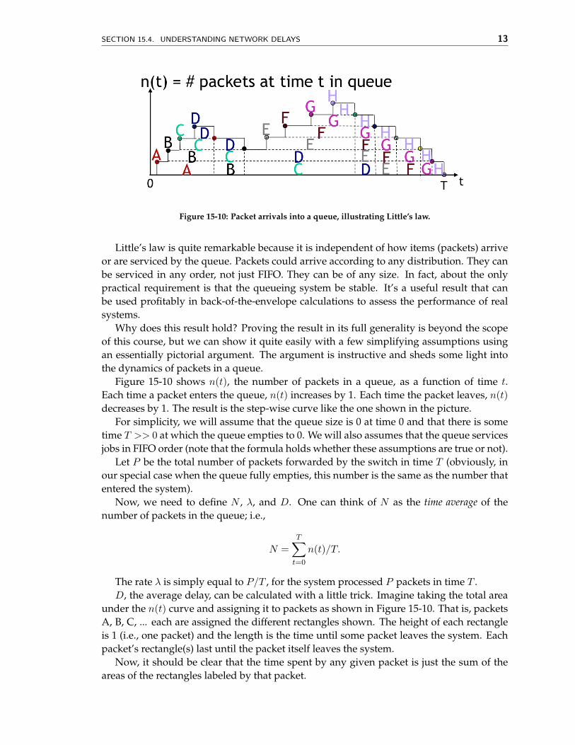
Figure 15-10: Packet arrivals into a queue, illustrating Little’s law.

Little’s law is quite remarkable because it is independent of how items (packets) arriveor are serviced by the queue. Packets could arrive according to any distribution. They canbe serviced in any order, not just FIFO. They can be of any size. In fact, about the onlypractical requirement is that the queueing system be stable. It’s a useful result that canbe used profitably in back-of-the-envelope calculations to assess the performance of realsystems.

Why does this result hold? Proving the result in its full generality is beyond the scopeof this course, but we can show it quite easily with a few simplifying assumptions usingan essentially pictorial argument. The argument is instructive and sheds some light intothe dynamics of packets in a queue.

Figure 15-10 shows n(t), the number of packets in a queue, as a function of time t.Each time a packet enters the queue, n(t) increases by 1. Each time the packet leaves, n(t)decreases by 1. The result is the step-wise curve like the one shown in the picture.

For simplicity, we will assume that the queue size is 0 at time 0 and that there is sometime T >> 0 at which the queue empties to 0. We will also assumes that the queue servicesjobs in FIFO order (note that the formula holds whether these assumptions are true or not).

Let P be the total number of packets forwarded by the switch in time T (obviously, inour special case when the queue fully empties, this number is the same as the number thatentered the system).

Now, we need to define N , λ, and D. One can think of N as the time average of thenumber of packets in the queue; i.e.,

N =T�

t=0

n(t)/T.

The rate λ is simply equal to P/T , for the system processed P packets in time T .D, the average delay, can be calculated with a little trick. Imagine taking the total area

under the n(t) curve and assigning it to packets as shown in Figure 15-10. That is, packetsA, B, C, ... each are assigned the different rectangles shown. The height of each rectangleis 1 (i.e., one packet) and the length is the time until some packet leaves the system. Eachpacket’s rectangle(s) last until the packet itself leaves the system.

Now, it should be clear that the time spent by any given packet is just the sum of theareas of the rectangles labeled by that packet.


Therefore, the average delay experienced by a packet, D, is simply the area under then(t) curve divided by the number of packets. That’s because the total area under the curve,which is

�n(t) is total delay experienced by all packets.

Hence,

D =T�

t=0

n(t)/P.

From the above expressions, Little’s law follows: N = λ×D.

� Problems and Questions

These questions are to help you improve your understanding of the concepts discussed inthis lecture. The ones marked *PSet* are in the online problem set. Some of these problemswill be discussed in recitation sections. If you need help with any of these questions, pleaseask anyone on the staff.

1. Under what conditions would circuit switching be a better network design thanpacket switching?

2. Which of these statements are correct?

(a) Switches in a circuit-switched network process connection establishment andtear-down messages, whereas switches in a packet-switched network do not.

(b) Under some circumstances, a circuit-switched network may prevent somesenders from starting new conversations.

(c) Once a connection is correctly established, a switch in a circuit-switched net-work can forward data correctly without requiring data frames to include adestination address.

(d) Unlike in packet switching, switches in circuit-switched networks do not needany information about the network topology to function correctly.

3. Consider a switch that uses time division multiplexing (rather than statistical multi-plexing) to share a link between four concurrent connections (A, B, C, and D) whosepackets arrive in bursts. The link’s data rate is 1 packet per time slot. Assume thatthe switch runs for a very long time.

(a) The average packet arrival rates of the four connections (A through D), in pack-ets per time slot, are 0.2, 0.2, 0.1, and 0.1 respectively. The average delays ob-served at the switch (in time slots) are 10, 10, 5, and 5. What are the averagequeue lengths of the four queues (A through D) at the switch?

(b) Connection A’s packet arrival rate now changes to 0.4 packets per time slot.All the other connections have the same arrival rates and the switch runs un-changed. What are the average queue lengths of the four queues (A through D)now?


4. *PSet* Over many months, you and your friends have painstakingly collected a 1,000Gigabytes (aka 1 Terabyte) worth of movies on computers in your dorm (we won’task where the movies came from). To avoid losing it, you’d like to back the data upon to a computer belonging to one of your friends in New York.

You have two options:

A. Send the data over the Internet to the computer in New York. The data rate fortransmitting information across the Internet from your dorm to New York is 1Megabyte per second.

B. Copy the data over to a set of disks, which you can do at 100 Megabytes persecond (thank you, firewire!). Then rely on the US Postal Service to send thedisks by mail, which takes 7 days.

Which of these two options (A or B) is faster? And by how much?

Note on units:

1 kilobyte = 103 bytes1 megabyte = 1000 kilobytes = 106 bytes1 gigabyte = 1000 megabytes = 109 bytes1 terabyte = 1000 gigbytes = 1012 bytes

5. Little’s law can be applied to a variety of problems in other fields. Here are somesimple examples for you to work out.

(a) F freshmen enter MIT every year on average. Some leave after their SB degrees(four years), the rest leave after their MEng (five years). No one drops out (yes,really). The total number of SB and MEng students at MIT is N .What fraction of students do an MEng?

(b) A hardware vendor manufactures $300 million worth of equipment per year.On average, the company has $45 million in accounts receivable. How muchtime elapses between invoicing and payment?

(c) While reading a newspaper, you come across a sentence claiming that “less than1% of the people in the world die every year”. Using Little’s law (and some commonsense!), explain whether you would agree or disagree with this claim. Assumethat the number of people in the world does not decrease during the year (thisassumption holds).

6. You send a stream of packets of size 1000 bytes each across a network path fromCambridge to Berkeley. You find that the one-way delay varies between 50 ms (inthe absence of any queueing) and 125 ms (full queue), with an average of 75 ms. Thetransmission rate at the sender is 1 Mbit/s; the receiver gets packets at the same ratewithout any packet loss.

A. What is the mean number of packets in the queue at the bottleneck link alongthe path (assume that any queueing happens at just one switch).


You now increase the transmission rate to 2 Mbits/s. You find that the receiver getspackets at a rate of 1.6 Mbits/s. The average queue length does not change apprecia-bly from before.

B. What is the packet loss rate at the switch?

C. What is the average one-way delay now?

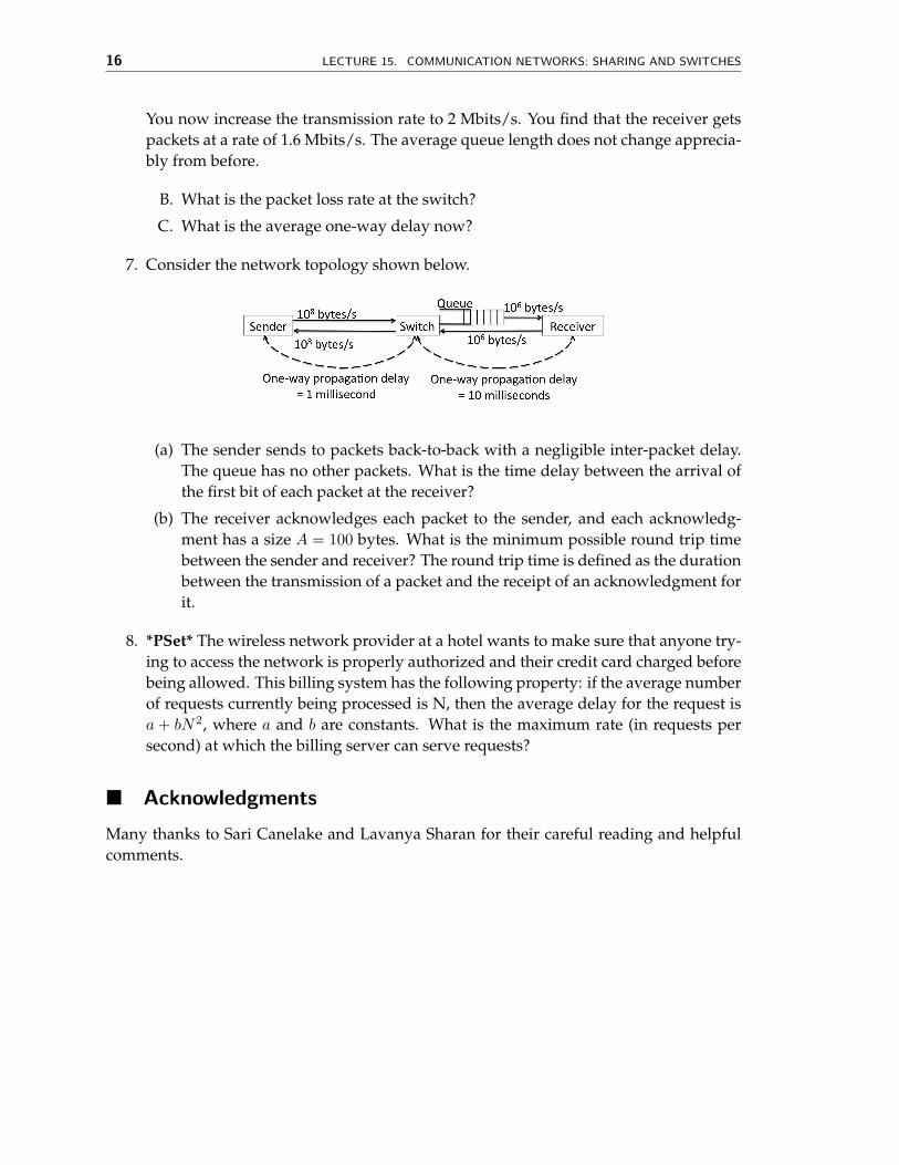
7. Consider the network topology shown below.

(a) The sender sends to packets back-to-back with a negligible inter-packet delay.The queue has no other packets. What is the time delay between the arrival ofthe first bit of each packet at the receiver?

(b) The receiver acknowledges each packet to the sender, and each acknowledg-ment has a size A = 100 bytes. What is the minimum possible round trip timebetween the sender and receiver? The round trip time is defined as the durationbetween the transmission of a packet and the receipt of an acknowledgment forit.

8. *PSet* The wireless network provider at a hotel wants to make sure that anyone try-ing to access the network is properly authorized and their credit card charged beforebeing allowed. This billing system has the following property: if the average numberof requests currently being processed is N, then the average delay for the request isa+ bN2, where a and b are constants. What is the maximum rate (in requests persecond) at which the billing server can serve requests?

� Acknowledgments

Many thanks to Sari Canelake and Lavanya Sharan for their careful reading and helpfulcomments.

Documents

ECTURE Communication Networks: Sharing and …web.mit.edu/6.02/www/s2010/handouts/lectures/L15-notes.pdf · communication networks: sharing and switches bit rate,5 of a link connected