Eddy current residual stress proﬁling in surface-treated ...pnagy/publications/Abu-Nabah et al., Nondestr. Test... · Eddy current residual stress proﬁling in surface-treated

Eddy current residual stress profiling in surface-treated engine alloys

Bassam A. Abu-Nabaha1, Feng Yua2, Waled T. Hassanb3, Mark P. Blodgettc and Peter B. Nagya*

aDepartment of Aerospace Engineering, University of Cincinnati, Cincinnati, OH 45221, USA; bHoneywellAerospace, Phoenix, AZ 85034, USA; cAir Force Research Laboratory, WPAFB, Dayton, OH 45433, USA

(Received 3 June 2008; final version received 3 June 2008 )

Recent research results indicate that eddy current conductivity measurements can be exploitedfor nondestructive evaluation of subsurface residual stresses in surface-treated nickel-basesuperalloy components. According to this approach, the depth-dependent electricconductivity profile is calculated from the measured frequency-dependent apparent eddycurrent conductivity spectrum. Then, the residual stress depth profile is calculated from theconductivity profile based on the piezoresistivity coefficient of the material, which isdetermined separately from calibration measurements using the known external appliedstresses. This paper reviews the basic principles, measurement procedures, advantages, andlimitations of eddy current residual stress profiling.

Keywords: eddy current; spectroscopy; surface-treatment; residual stress profiling

1. Introduction

Nondestructive residual stress assessment in fracture-critical components is one of the most

promising opportunities and difficult challenges we face in the NDE community today. Residual

stress assessment is important because there is mounting evidence that it is not possible to reliably

and accurately predict the remaining service life of such components without properly accounting

for the presence of residual stresses.Unfortunately, both the absolute level and spatial distribution of

the residual stress are rather uncertain, partly because the stress is highly susceptible to variations in

the manufacturing process and subsequently it tends to undergo thermo-mechanical relaxation at

operating temperatures. Therefore, the only reliable way to establish the actual level and spatial

profile of the prevailing residual stress is by measuring them. Unfortunately, the only currently

available NDE method for residual stress assessment is based on X-ray diffraction (XRD)

measurement that is limited to an extremely thin, less than 20mm deep, surface layer [1–4]. In this

study, to get the necessary information on the subsurface residual stresses destructive XRD

measurements were conducted on selected specimens following the nondestructive eddy current

conductivity measurements. The XRD method is routinely used to measure subsurface residual

stresses via repeated removal of thin surface layers by electro-polishing.When such layer removal is

performed, the measured stress needs to be corrected for the stress relaxation and redistribution that

occurs because of layer removal [5,6].

The peak diffraction direction is determined by the absolute elastic strain in the material.

At the same time, as a by-product of this measurement, we also get some information on the

plastic deformation in the material because the widening of the diffraction peak is due to the lack

of periodicity in the lattice, which is related to dislocation density and other lattice

ISSN 1058-9759 print/ISSN 1477-2671 online

q 2009 Taylor & Francis

DOI: 10.1080/10589750802245280

http://www.informaworld.com

*Corresponding author. Email: [email protected]

Nondestructive Testing and Evaluation,Vol. 24, Nos. 1–2, March–June 2009, 209–232

Downloaded By: [Nagy, Peter B.] At: 01:49 24 December 2008

imperfections. However, in order to evaluate the whole compressive part of the subsurface

residual stress profile using XRD measurements, successive layer removal has to be applied,

which requires some numerical corrections to account for the inevitable stress release during this

process. This method is inherently destructive since it leaves a deep hole on the surface.

Although the accuracy of XRD measurements is quite sufficient for life prediction purposes, the

necessity of surface layer removal for subsurface measurements essentially excludes the use of

this method as a nondestructive characterisation tool.

There are really only twoways to avoid this limitation ofXRD, namely either by increasing the

incident beam intensity or by reducing the wave length, which then reduces the X-ray absorption

coefficient of the material so that one gets better penetration. Today, this can be achieved only by

using either synchrotron radiation or neutron diffraction, which could increase the penetration

depth to a few centimetres [7,8]. On the negative side, the spatial resolution of these methods

leaves much to be desired since a minimum diffraction volume must be maintained to reach

sufficient sensitivity and that translates into a depth resolution on the order of 100mm. That is still

enough, although barely, for surface-treated components, even for shot-peened oneswhich exhibit

rather shallow compressive residual stress layers. Of course, it is a major disadvantage of these

techniques that they require access to a synchrotron accelerator or a nuclear reactor.

Surface enhancement methods, such as shot peening (SP), laser shock peening (LSP), and

low-plasticity burnishing (LPB), significantly improve the fatigue resistance and foreign object

damage tolerance of metallic components by introducing beneficial near-surface compressive

residual stresses. Moreover, the surface is slightly strengthened and hardened by the

cold-working process. By far the most common way to produce protective surface layers of

compressive residual stress is by SP, though it is probably also the worst technique from the

point of view of damaging cold work which substantially decreases the thermo-mechanical

stability of the microstructure at elevated operating temperatures and leads to accelerated

relaxation of the beneficial residual stresses [2]. Although LSP and LPB produces significiantly

deeper compressive residual stress than SP, their main advantage over SP is that they produce

much less cold work on the order of 5–15% equivalent plastic strain.

2. Eddy current conductivity spectroscopy

Because of the above discussed limitations, the NDE community has been looking for

alternatives to assess residual stress profiles in surface-treated engine components for many

years and eddy current conductivity spectroscopy emerged as one of the leading candidates

[9–28]. Eddy current residual stress profiling is based on the piezoresistivity of the material, i.e.,

on the characteristic dependence of the electric conductivity on stress. Figure 1 shows a

schematic representation of physics-based eddy current residual stress profiling in surface-

treated components. In order to remove the influence of the measurement system (coil size,

shape, etc.) the actually measured complex electric impedance of the probe coil is first

transformed into a so-called apparent eddy current conductivity (AECC) parameter. At a given

inspection frequency, the AECC is defined as the electric conductivity of an equivalent

homogeneous, non-magnetic, smooth, and flat specimen placed at a properly chosen distance

from the coil that would produce the same complex electric coil impedance as the

inhomogeneous specimen under study [19].

If spurious material (e.g., magnetic permeability) and geometric (e.g., surface roughness)

variations can be neglected, the frequency-dependent AECC can be inverted for the

depth-dependent electric conductivity profile (this principal path is highlighted in Figure 1).

Then, using the known piezoresistivity of the material, the sought residual stress profile can be

calculated. Unfortunately, the measured complex electric coil impedance, and therefore also the

B.A. Abu-Nabah et al.210


inferred AECC, is affected by the presence of cold work and surface roughness as well as by the

sought near-surface residual stress. The electric conductivity variation due to residual stress is

usually weak (<1%) and rather difficult to separate from these accompanying spurious effects.

In certain materials, such as austenitic stainless steels, cold work might also cause significant

magnetic permeability variation which affects the measured coil impedance. Fortunately,

nickel-base superalloys do not exhibit such ferromagnetic transition from their paramagnetic

state [22]. In addition, because of their significant hardness, shot-peened nickel-base superalloy

components exhibit only rather limited surface roughness (<2–3mm rms), therefore the

influence of geometrical irregularities is also limited. Still, as the inspection frequency increases

the eddy current loop becomes squeezed closer to the rough surface, which creates a more

tortuous, therefore longer, path and might lead to a perceivable drop of AECC above

30–40MHz [29–31].

In order to translate the measured frequency-dependent AECC into a depth-dependent

electric conductivity profile in a non-magnetic medium, first a simplistic inversion technique

was developed [20], which was recently followed by the development of a highly convergent

iterative inversion technique [23]. Both techniques indicated that at any given frequency the

measured AECC corresponds roughly to the actual electric conductivity at half of the standard

penetration depth assuming that: (i) the electric conductivity variation is limited to a shallow

surface region of depth much less than the probe coil diameter, (ii) the relative change in electric

conductivity is less than a few percents, and (iii) the electric conductivity depth profile is

continuous and fairly smooth. Alternatively, best fitting of the measured electric coil impedance

with the known analytical solution can be used assuming that the conductivity profile can be

characterised by a small number of independent parameters [28]. Finally, the sought residual

Figure 1. A schematic representation of physics-based eddy current residual stress profiling in surface-treated components (the principal path is highlighted).

Nondestructive Testing and Evaluation 211


stress profile is calculated from the electric conductivity profile based on the piezoresistivity

coefficient of the material, which is determined separately from the material calibration

measurements using the known external applied stresses.

2.1 Material calibration, piezoresistivity

In the presence of elastic stress t the electrical conductivity s tensor of an isotropic conductor

becomes slightly anisotropic. In general, the stress-dependence of the electrical resistivity can be

described by the fourth-order piezoresistivity tensor [32–38]. In direct analogy to the well-

known acoustoelastic coefficients, the widely used NDE terminology for the stress coefficient of

the acoustic velocity, the stress coefficient of the electrical conductivity is referred to as the

electroelastic coefficient.

Ds1=s0

Ds2=s0

Ds3=s0

2664

3775 ¼

k11 k12 k12

k12 k11 k12

k12 k12 k11

2664

3775

t1=E

t2=E

t3=E

2664

3775: ð1Þ

Here, E denotes Young’s modulus, Dsi ¼ si 2 s0 (i ¼ 1,2,3) denotes the conductivity change

due to the presence of stress, s0 denotes the electrical conductivity in the absence of stress, and k11andk12 are the unitless parallel andnormal electroelastic coefficients, respectively.Duringmaterials

calibration, directional racetrack [39] or meanderising [40] probe coils can be used to measure the

parallel k11 and normal k12 electroelastic coefficients essentially independent of each other. In the

case of shot-peened or otherwise treated surfaces, essentially isotropic plane stress (t1 ¼ t2 ¼ tipand t3 ¼ 0) condition prevails. Then, regardless whether conventional non-directional circular

or directional probes are used, the effective electroelastic coefficient is kip ¼ k11 þ k12.

As it was illustrated in Figure 1, the electric conductivity is sensitive to both elastic strains

caused by the prevailing residual stress state and plastic strains produced by prior coldwork, i.e., it

lacks the selectivity to separate these two principal effects of surface treatment. This is rather

unfortunate, but not unusual at all in nondestructive evaluation which often has to rely on indirect

measurements to remain nondestructive. Since the effects of cold work and associated

microstructural changes are not fully understood at this point, the electric conductivity depth

profiles will be converted into estimated residual stress profiles based solely on the piezoelectric

effect according to equation (1). It will be shown that completely neglecting cold work effects

causes a systematic error in the estimated residual stress profiles. The simplest way to account for

cold work effects is to use empirically corrected electroelastic coefficients instead of the

calibration values independently measured under purely elastic deformation [21]. The necessary

empirical correction then indicates the relative contribution of the otherwise unaccounted for cold

work effects rather than the uncertainty of the electroelastic coefficient obtained by calibration.

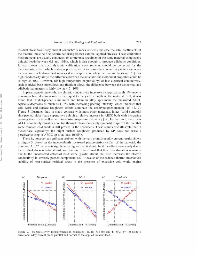
Figure 2 shows examples of piezoresistivity measurements in Waspaloy, IN718, and

Ti–6Al–4V engine materials using a directional eddy current probe parallel and normal to the

applied uniaxial load. Here, the normalised change in conductivity Ds/s0 is plotted against the

uniaxial strain 1ua ¼ tua/E. In some materials, such as Ti–6Al–4V, the parallel and normal

electroelastic coefficients are more or less equal in magnitude and opposite in sign, which

renders the eddy current conductivity measurements essentially useless for residual stress

assessment in the case of isotropic plane stress on surface-treated components. However, there is

a very important group of materials, notably nickel-base superalloys, where the two coefficients

have similar magnitudes and signs, therefore the parallel and normal effects reinforce each other

to produce a fairly significant stress-dependence. In order to quantitatively assess the prevailing



residual stress from eddy current conductivity measurements, the electroelastic coefficients of

the material must be first determined using known external applied stresses. These calibration

measurements are usually conducted on a reference specimen of the same material using cyclic

uniaxial loads between 0.1 and 10Hz, which is fast enough to produce adiabatic conditions.

It was shown that such dynamic calibration measurements should be corrected for the

thermoelastic effect, which is always positive, i.e., it increases the conductivity in tension, when

the material cools down, and reduces it in compression, when the material heats up [21]. For

high-conductivity alloys the difference between the adiabatic and isothermal properties could be

as high as 50%. However, for high-temperature engine alloys of low electrical conductivity,

such as nickel-base superalloys and titanium alloys, the difference between the isothermal and

adiabatic parameters is fairly low at <5–10%.

In paramagnetic materials, the electric conductivity increases by approximately 1% under a

maximum biaxial compressive stress equal to the yield strength of the material. Still, it was

found that in shot-peened aluminium and titanium alloy specimens the measured AECC

typically decreases as much as 1–2% with increasing peening intensity, which indicates that

cold work and surface roughness effects dominate the observed phenomenon [15–17,19].

Figure 3 illustrates that, in sharp contrast with most other materials, intact (solid symbols)

shot-peened nickel-base superalloys exhibit a relative increase in AECC both with increasing

peening intensity as well as with increasing inspection frequency [19]. Furthermore, the excess

AECC completely vanishes upon full thermal relaxation (empty symbols) in spite of the fact that

some remnant cold work is still present in the specimens. These results also illustrate that in

nickel-base superalloys the slight surface roughness produced by SP does not cause a

perceivable drop of AECC up to at least 10MHz.

There is, however, a significant problem with the very promising eddy current results shown

in Figure 3. Based on the independently measured piezoresistivity effect of the material, the

observed AECC increase is significantly higher than it should be if the effect were solely due to

the residual stress (elastic strain) contribution. It was found that this overestimation is mainly

due to the uncorrected effect of cold work (plastic strain) that also increases the electric

conductivity in severely peened components [22]. Because of the reduced thermo-mechanical

stability of near-surface residual stress in the presence of excessive cold work, engine

Figure 2. Piezoresistivity measurements in Waspaloy (a), IN 718 (b) and Ti–6Al–4V (c) using adirectional eddy current probe parallel and normal to the applied uniaxial load.



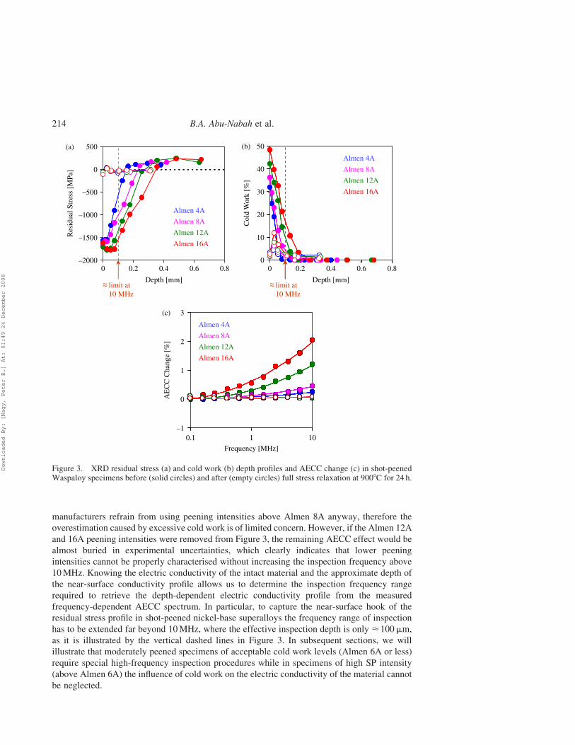
manufacturers refrain from using peening intensities above Almen 8A anyway, therefore the

overestimation caused by excessive cold work is of limited concern. However, if the Almen 12A

and 16A peening intensities were removed from Figure 3, the remaining AECC effect would be

almost buried in experimental uncertainties, which clearly indicates that lower peening

intensities cannot be properly characterised without increasing the inspection frequency above

10MHz. Knowing the electric conductivity of the intact material and the approximate depth of

the near-surface conductivity profile allows us to determine the inspection frequency range

required to retrieve the depth-dependent electric conductivity profile from the measured

frequency-dependent AECC spectrum. In particular, to capture the near-surface hook of the

residual stress profile in shot-peened nickel-base superalloys the frequency range of inspection

has to be extended far beyond 10MHz, where the effective inspection depth is only <100mm,

as it is illustrated by the vertical dashed lines in Figure 3. In subsequent sections, we will

illustrate that moderately peened specimens of acceptable cold work levels (Almen 6A or less)

require special high-frequency inspection procedures while in specimens of high SP intensity

(above Almen 6A) the influence of cold work on the electric conductivity of the material cannot

be neglected.

Figure 3. XRD residual stress (a) and cold work (b) depth profiles and AECC change (c) in shot-peenedWaspaloy specimens before (solid circles) and after (empty circles) full stress relaxation at 9008C for 24 h.



2.2 Instrument calibration

Most eddy current inspections are conducted in one of two basic modes of operation, namely in

‘impedance’ and ‘conductivity’ modes. In the so-called conductivity mode, which is most often

used for alloy sorting and quantitative characterisation of metals, the measured probe coil

impedance is evaluated for an ‘apparent’ eddy current conductivity G( f) and ‘apparent’ lift-off

distance ‘( f) by assuming that the specimen is a sufficiently large homogeneous non-magnetic

conductor, even when it is actually not. At a given frequency f and hypothetical lift-off distance

‘( f), a hypothetical material of conductivity G( f) would produce exactly the same complex coil

impedance as the real specimen under test. Complications such as inhomogeneity, permeability

effects, surface roughness, etc., are neglected during inversion of the coil impedance, therefore

the thereby measured quantity will be referred to as AECC. Existing differences between the

actual specimen and an ideal homogeneous non-magnetic conductor exert a convoluted effect on

the measured AECC and make it frequency-dependent. Of course, the intrinsic electrical

conductivity of the material is independent of frequency. In the case of layered or otherwise

inhomogeneous specimens the observed frequency-dependence of the AECC is due to the

depth-dependence of the electrical conductivity or magnetic permeability and the

frequency-dependence of the eddy current penetration depth. Furthermore, near-surface defects

and spurious surface roughness could also cause an additional frequency-dependent loss of eddy

current conductivity.

For a given set of vertical and horizontal gains and phase rotation, the real and imaginary

components of the measured complex impedance are determined by the electric conductivity of

the specimen and the lift-off distance. For the purposes of instrument calibration, four reference

points are measured on two appropriate calibration blocks (s1 and s2) with (‘ ¼ s) and without

(‘ ¼ 0) a polymer foil of thickness s between the probe coil and the specimens. The coil

impedance measured on the shot-peened specimen is then evaluated in terms of apparent

conductivity and lift-off using simple linear interpolation, though the lift-off data is often

discarded. It should be mentioned that the linear interpolation technique, which is known to

leave much to be desired over larger conductivity ranges, is quite sufficient over the relatively

small range considered in this study unless the inspection frequency exceeds 20MHz. Later, we

will show that at high inspection frequencies efficient rejection of inevitable lift-off variations is

of the utmost importance because of the high precision requirements of these measurements and

better lift-off rejection requires nonlinear interpolation.

In the conductivity mode of operation, the measured frequency-dependent complex electric

impedance of the coil is first translated into an AECC spectrum as it was shown schematically in

Figure 1, which is then inverted into a frequency-independent depth profile of the electric

conductivity, as it will be shown in the next section. The main advantage of this two-step

approach is that it effectively eliminates the influence of the measurement system on the actually

measured coil impedance, therefore AECC spectra taken with different equipments and different

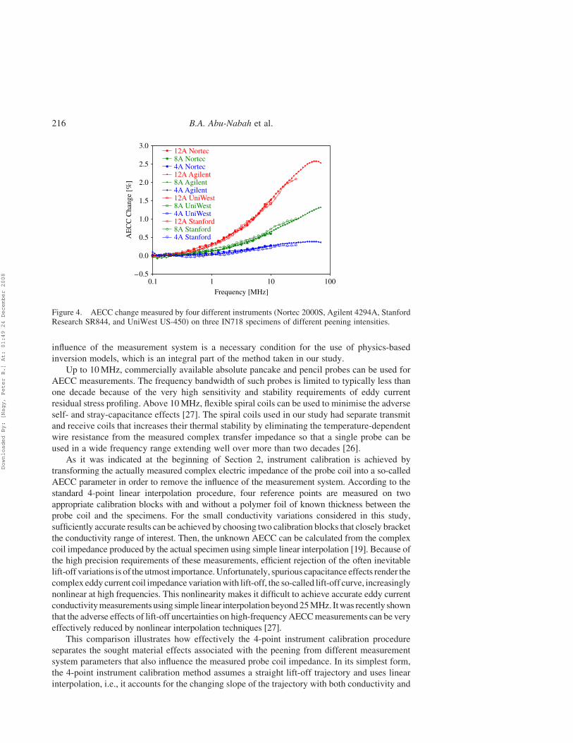
probe coils can be directly compared. To illustrate the robustness of this instrument calibration

method, Figure 4 shows the AECC spectra measured by four different instruments (Nortec

2000S, Agilent 4294A, Stanford Research SR844, and UniWest US-450) on three IN718

specimens of different peening intensities. In the overlapping frequency ranges the agreement

between the AECC spectra obtained by different instruments is within the respective estimated

errors of the instruments. Of course, true physical quantities do not depend on the way they are

measured. However, eddy current conductivity measurements are inherently susceptible to

influence by the measurement system because of the complex relationship between the true

material parameter, i.e., the depth-dependent electric conductivity, and the measured physical

parameter, i.e., the frequency-dependent AECC. Independence of the measured AECC from the



influence of the measurement system is a necessary condition for the use of physics-based

inversion models, which is an integral part of the method taken in our study.

Up to 10MHz, commercially available absolute pancake and pencil probes can be used for

AECC measurements. The frequency bandwidth of such probes is limited to typically less than

one decade because of the very high sensitivity and stability requirements of eddy current

residual stress profiling. Above 10MHz, flexible spiral coils can be used to minimise the adverse

self- and stray-capacitance effects [27]. The spiral coils used in our study had separate transmit

and receive coils that increases their thermal stability by eliminating the temperature-dependent

wire resistance from the measured complex transfer impedance so that a single probe can be

used in a wide frequency range extending well over more than two decades [26].

As it was indicated at the beginning of Section 2, instrument calibration is achieved by

transforming the actually measured complex electric impedance of the probe coil into a so-called

AECC parameter in order to remove the influence of the measurement system. According to the

standard 4-point linear interpolation procedure, four reference points are measured on two

appropriate calibration blocks with and without a polymer foil of known thickness between the

probe coil and the specimens. For the small conductivity variations considered in this study,

sufficiently accurate results can be achieved by choosing two calibration blocks that closely bracket

the conductivity range of interest. Then, the unknown AECC can be calculated from the complex

coil impedance produced by the actual specimen using simple linear interpolation [19]. Because of

the high precision requirements of these measurements, efficient rejection of the often inevitable

lift-off variations is of the utmost importance.Unfortunately, spurious capacitance effects render the

complex eddy current coil impedance variationwith lift-off, the so-called lift-off curve, increasingly

nonlinear at high frequencies. This nonlinearity makes it difficult to achieve accurate eddy current

conductivitymeasurements using simple linear interpolationbeyond25MHz. Itwas recently shown

that the adverse effects of lift-off uncertainties on high-frequencyAECCmeasurements can be very

effectively reduced by nonlinear interpolation techniques [27].

This comparison illustrates how effectively the 4-point instrument calibration procedure

separates the sought material effects associated with the peening from different measurement

system parameters that also influence the measured probe coil impedance. In its simplest form,

the 4-point instrument calibration method assumes a straight lift-off trajectory and uses linear

interpolation, i.e., it accounts for the changing slope of the trajectory with both conductivity and

Figure 4. AECC change measured by four different instruments (Nortec 2000S, Agilent 4294A, StanfordResearch SR844, and UniWest US-450) on three IN718 specimens of different peening intensities.



frequency, which makes it more suitable for precision measurements. Above 20MHz, where

inevitable lift-off variations adversely influence the accuracy of the AECC measurement,

nonlinear interpolation must be used to achieve the same stringent requirements of about 0.1%

relative accuracy.

2.3 AECC inversion

The measured frequency-dependent AECC must be inverted into a depth-dependent electric

conductivity profile before it can be converted into the sought residual stress profile using the known

piezoelectric parameter of thematerial. Because of the limited accuracy of both theAECCspectrum

and the approximations used to relate conductivity to stress, a simplistic inversion technique will

suffice in most cases [20]. According to this approach, at any given frequency the measured AECC

corresponds roughly to the actual electric conductivity at half of the standard penetration depth. It

might seem highly unlikely that such a simplistic inversion procedure could reasonably predict the

actual conductivity profile from themeasured frequency-dependent AECC,G( f). Indeed, generally,

this simplistic inversionmethodyields rather poor results.However, even in extreme cases, such as a

rectangular profile representing a uniform layer of increased conductivity on a homogeneous

substrate, the peak conductivity and half-peak penetration depth of the reconstructed profile are both

well-reconstructed. When necessary, much more accurate inversion can be achieved by iterative

application of the same principle in a feed-back loop that relies on the outstanding accuracy and

speed of the 1D forward approximation of the electromagnetic problem [23]. The iterative in version

technique is numerically stable as long as the random variations of the AECC spectrum remain

below ^0.1%. Beyond this level, the robustness of the iterative inversion procedure is adversely

affected by random variations in the AECC spectrum. In such cases smoothening of the measured

AECC profile can be used to eliminate potential inversion instabilities.

3. Measurement limitations

The main limitation of residual stress profiling by eddy current conductivity spectroscopy is that

the feasibility of this technique seems to be limited to nickel-base superalloys, though some

beneficial information, e.g., on increasing hardness, could be also obtained by this technique on

titanium and aluminium alloys. Unfortunately, even in the case of nickel-base superalloys, there

exist some serious limitations that adversely influence the applicability of the eddy current

method. In this chapter, three such adverse effects will be reviewed. First, forged nickel-base

superalloys often exhibit significant conductivity inhomogeneity that could interfere with

subsurface residual stress characterisation. Second, these materials are susceptible to cold-work-

induced microstructural changes that cause a conductivity increase similar or even larger than

the primary conductivity increase caused by compressive residual stresses. Third, the electrical

conductivity in nickel-base superalloys is rather low (<1.5% IACS), therefore the standard

penetration depth is relatively high at a given frequency (<180mm at 10MHz). Therefore, we

cannot fully reconstruct the critical near-surface part of the residual stress profile in moderately

peened components using only typical inspection frequencies below 10MHz. In such cases,

special high-frequency inspection techniques are needed to extend the frequency range up to

50–80MHz, i.e., beyond the range of commercially available instruments.

3.1 Inhomogeneity effect

Surface-treated nickel-base superalloys exhibit an approximately 1% increase in AECC at high

inspection frequencies, which can be exploited for nondestructive subsurface residual stress

assessment. Unfortunately, microstructural inhomogeneity in certain as-forged and precipitation



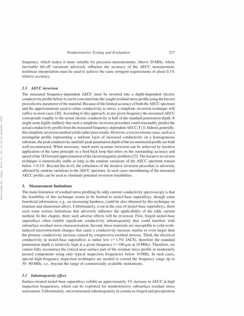
hardened nickel-base superalloys, like Waspaloy, can lead to significantly larger electrical

conductivity variations of as much as 4–6%. Figure 5 shows examples of typical eddy current

conductivity images from inhomogeneous Waspaloy specimens and homogeneous IN100

specimens taken at 6MHz. The as-forged Waspaloy specimens were 53 £ 107mm and

exhibited a wide conductivity range from 1.38 to 1.47% IACS, or ^3.2% in relative terms.

In contrast, the 28 £ 56mm powder metallurgic IN100 specimens exhibited a very narrow

conductivity range from 1.337 to 1.341% IACS or ^0.13% in relative terms. It should be

mentioned that images of IN718 specimens revealed a medium level of inhomogeneity. It is

postulated that the observed electrical inhomogeneity difference between Waspaloy, IN718, and

IN100 is caused by their different alloy composition and thermo-mechanical processing and it is

somehow related to the microstructure of these materials.

The roughly 3–4% electrical conductivity variation exhibited by inhomogeneous Waspaloy

specimens raises a crucial question: Can eddy current techniques detect, let alone quantitatively

characterise, the weaker near-surface conductivity variations caused by surface treatment in the

presence of this much stronger conductivity inhomogeneity caused by microstructural

variations? Eddy current conductivity images taken at different inspection frequencies indicated

that low- and high-conductivity domains are essentially frequency independent due the large

volumetric size of these domains [25]. This virtual frequency independence can be exploited to

distinguish these inhomogeneities from near-surface residual stress and cold work effects caused

by surface treatment, which, in contrast, are strongly frequency-dependent. As the frequency

decreases, the eddy current penetrates deeper into the material and also spreads a little wider in

the radial direction. Although there is some change in the AECC with frequency at most

locations, on average this frequency-dependence essentially cancels out for a large number of

points.

The rather weak frequency-dependence of the inhomogeneity-induced AECC variation

suggests that the conductivity does not vary sharply with depth, which can be exploited

Figure 5. Examples of the AECC maps of unpeened inhomogeneous as-forged Waspaloy specimens(a) and homogeneous powder metallurgic IN100 specimens (b) at 6MHz.



to separate the primary residual stress effect from the spurious material inhomogeneity using

point-by-point absolute AECC measurements over a wide frequency range, followed by a

comparison of the near-surface properties measured at high frequencies to those at larger depth

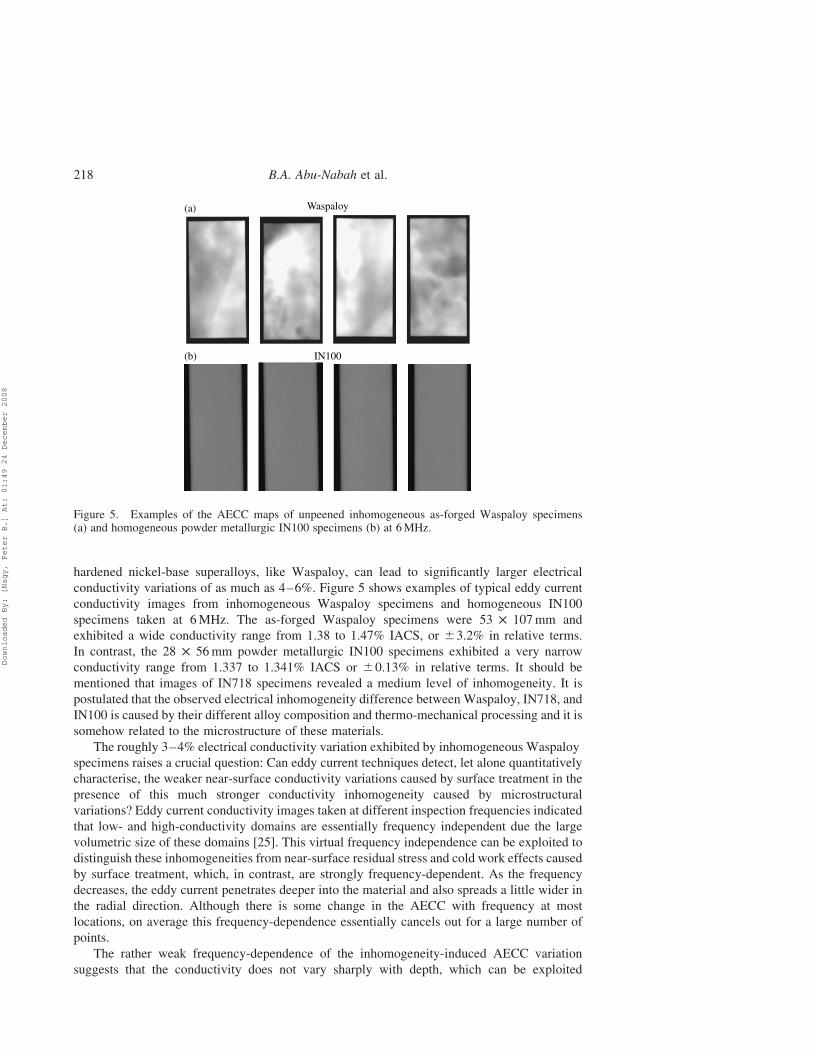
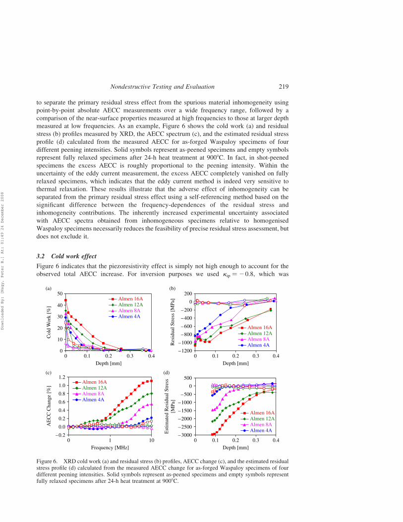
measured at low frequencies. As an example, Figure 6 shows the cold work (a) and residual

stress (b) profiles measured by XRD, the AECC spectrum (c), and the estimated residual stress

profile (d) calculated from the measured AECC for as-forged Waspaloy specimens of four

different peening intensities. Solid symbols represent as-peened specimens and empty symbols

represent fully relaxed specimens after 24-h heat treatment at 9008C. In fact, in shot-peened

specimens the excess AECC is roughly proportional to the peening intensity. Within the

uncertainty of the eddy current measurement, the excess AECC completely vanished on fully

relaxed specimens, which indicates that the eddy current method is indeed very sensitive to

thermal relaxation. These results illustrate that the adverse effect of inhomogeneity can be

separated from the primary residual stress effect using a self-referencing method based on the

significant difference between the frequency-dependences of the residual stress and

inhomogeneity contributions. The inherently increased experimental uncertainty associated

with AECC spectra obtained from inhomogeneous specimens relative to homogenised

Waspaloy specimens necessarily reduces the feasibility of precise residual stress assessment, but

does not exclude it.

3.2 Cold work effect

Figure 6 indicates that the piezoresistivity effect is simply not high enough to account for the

observed total AECC increase. For inversion purposes we used kip ¼ 20.8, which was

Figure 6. XRD cold work (a) and residual stress (b) profiles, AECC change (c), and the estimated residualstress profile (d) calculated from the measured AECC change for as-forged Waspaloy specimens of fourdifferent peening intensities. Solid symbols represent as-peened specimens and empty symbols representfully relaxed specimens after 24-h heat treatment at 9008C.



measured on a reference specimen cut from the same batch of material. A comparison of the

scales in Figure 6 (b, d) reveals that the inverted residual stress significantly overestimates the

more reliable XRD results. It should be mentioned that the overestimation is much lower in

IN718 and, especially, in IN100.

The most probable reason for the observed overestimation is the influence of cold work.

In order to better understand the effects of cold work on the AECC change in shot-peened

nickel-base superalloys, the effect of plastic deformation on the electrical conductivity, magnetic

permeability, and electroelastic coefficient of premium grade rotor-quality nickel-base

superalloys was investigated in detail [22]. The results indicated that, within the uncertainty of

the measurement, the electroelastic coefficient and the magnetic permeability do not change as a

result of cold work, therefore they cannot be responsible for the significant overestimation of the

residual stress described above. On the other hand, the electric conductivity did show significant

variation with plastic strain in cold-worked nickel-base superalloys. The substantial increase of

the electrical conductivity is due to microstructural changes and could explain the observed

residual stress overestimation. Of course, the cold work produced by SP rapidly decays away

from the surface and the depth of the affected layer is typically only 30% of the thickness of the

layer of compressive residual stress. Therefore, at frequencies below 10MHz the overestimation

tends to be less than what could be expected based on the sheer magnitudes of these two effects.

Cold work exerts a very convoluted effect on residual stress profiling by eddy current

spectroscopic measurements and will require further research to better understand its behaviour

and to develop possible compensation strategies. However, it should be pointed out that the

overestimation of the eddy current method due to cold work is much lower in moderately peened

components, which exhibit better thermo-mechanical stability, and in LSP and LPB specimens,

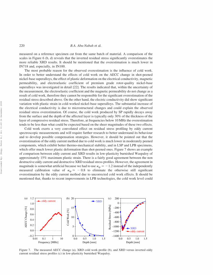
which offer much lower plastic deformation than shot-peened ones. Figure 7 shows an example

of comparison between eddy current and XRD results in low-plasticity burnished Waspaloy of

approximately 15% maximum plastic strain. There is a fairly good agreement between the non

destructive eddy current and destructive XRD residual stress profiles. However, the agreement in

magnitude is somewhat artificial because we had to use kip ¼ 21.2 instead of the independently

measured calibration value of kip < 2 0.8 to eliminate the otherwise still significant

overestimation by the eddy current method due to uncorrected cold work effects. It should be

mentioned that, thanks to recent improvements in LPB technologies, the cold work level could

Figure 7. The measured AECC change (a), XRD cold work profile (b), and XRD versus inverted eddycurrent residual stress profiles (c) in low-plasticity burnished Waspaloy.



be reduced to less than 5%, which would further reduce the need for such empirical corrections

that depend on material properties as well as on the type of surface treatment.

3.3 High-frequency inspection

The main reason for choosing peening intensities in excess of typical levels recommended by

engine manufacturers in early studies was that the eddy current penetration depth could not be

sufficiently decreased without extending the frequency range above 10MHz, i.e., beyond

the operational range of most commercially available eddy current instruments. In contrast, in

the case of eddy current residual stress profiling in shot-peened nickel-base superalloys, the

inspection frequency has to be extended to at least 50MHz to capture the important part of the

near-surface residual stress profile. For this purpose, we adapted an Agilent 4294A

high-precision impedance analyser to eddy current conductivity spectroscopy [26]. The eddy

current system based on this instrument offers better stability, reproducibility, and measurement

speed than the formerly used commercial eddy current instruments. Spiral coils made on

polymer foils offer high resonance frequency, thereby making them suitable for operation at

high inspection frequencies [41,42]. Using separate transmit and receive coils improves the

probe coil’s thermal stability by eliminating the temperature-dependent coil resistance from the

measured electric impedance.

Unfortunately, spurious capacitive effects render the lift-off trajectory of the probe coils

more nonlinear at high frequencies and make it rather difficult to achieve accurate AECC

measurements above 25MHz [27]. The inductive and capacitive effects on the lift-off sensitivity

of the probe coil are opposite. The inductive effect dominates below 20MHz, i.e., at typical eddy

current inspection frequencies. Both effects increase with frequency with the inductive effect

being initially stronger, but then it is taken over at high frequencies by the faster growing

capacitive effect. Since the two effects produce opposite curvature in the lift-off trajectory, in the

frequency range where they are approximately equal the lift-off trajectory becomes essentially

linear and very accurate conductivity measurements can be conducted even in the presence of

substantial lift-off variations.

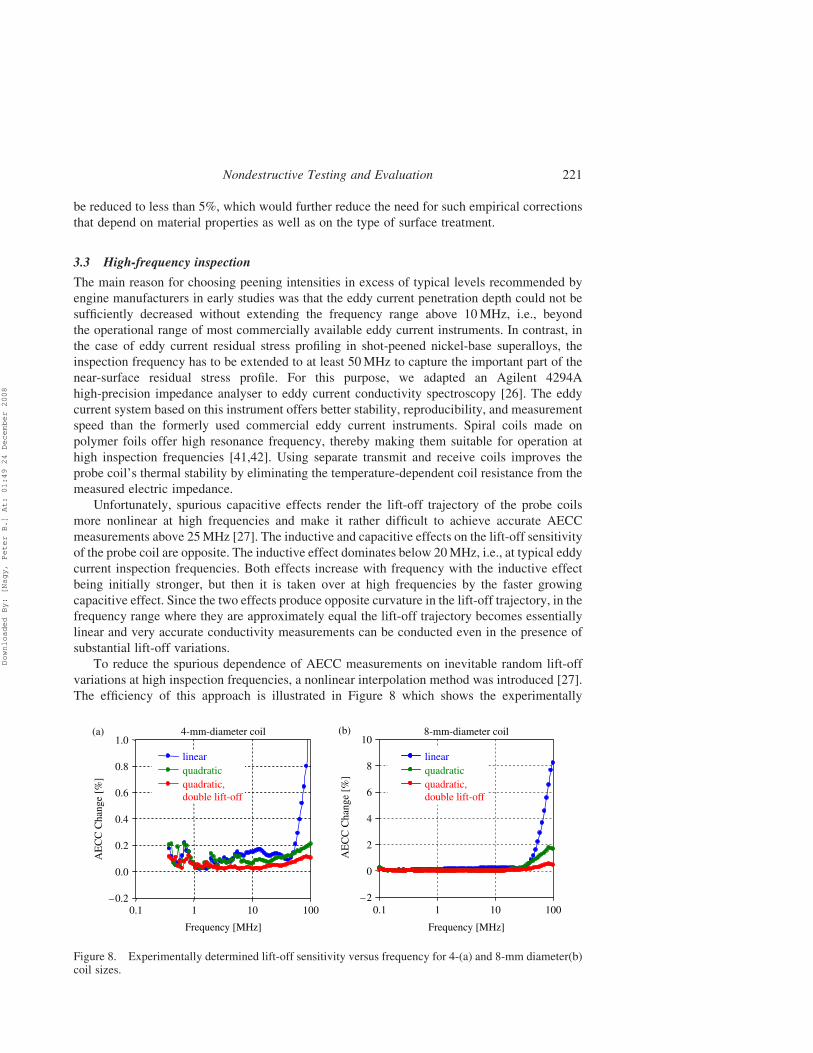
To reduce the spurious dependence of AECC measurements on inevitable random lift-off

variations at high inspection frequencies, a nonlinear interpolation method was introduced [27].

The efficiency of this approach is illustrated in Figure 8 which shows the experimentally

Figure 8. Experimentally determined lift-off sensitivity versus frequency for 4-(a) and 8-mm diameter(b)coil sizes.



determined lift-off sensitivity versus frequency for 4- and 8-mm diameter coils. In this paper,

these flat spiral coils are referred to simply by their outer diameter, which is exactly twice their

inner diameter. The width of the conducting strip and the air gap between neighbouring turns

was kept constant at 0.1mm. Computational simulation was conducted to study the sensitivity of

these coils using the commercially available Vic-3d program [27]. The simulations were found

to be in good agreement for the conductivity sensitivity over the whole frequency range from 0.1

to 100MHz and for the lift-off sensitivity from 0.1MHz up to about 20MHz. At higher

frequencies the lift-off sensitivity becomes a crucial issue that can compromise the accuracy of

conductivity measurements in the presence of lift-off uncertainties as small as 0.05mm. Above

20MHz, the purely inductive Vic-3D simulation greatly underestimated the experimentally

observed lift-off sensitivity of these probe coils. It was shown that the increasing susceptibility

of conductivity measurements to lift-off variations is due to capacitive effects that are not

accounted for in the simulation. Therefore, a simple lumped-element analytical simulation was

suggested to better understand the underlying physical phenomenon [27]. Further research is

needed to develop numerical tools that properly incorporate self- and stray-capacitance effects

into the eddy current simulation.

Figure 8 illustrates that the lift-off rejection is much better for the smaller probe (the vertical

scales are different by a factor of 10) and when quadratic interpolation is used for instrument

calibration. Furthermore, in the latter case, the rejection can be further improved by extending

the calibration lift-off range since the curvature is more accurately measured over a larger

distance. In contrast, in the case of linear interpolation the lift-off rejection decreases with

increasing lift-off calibration range.

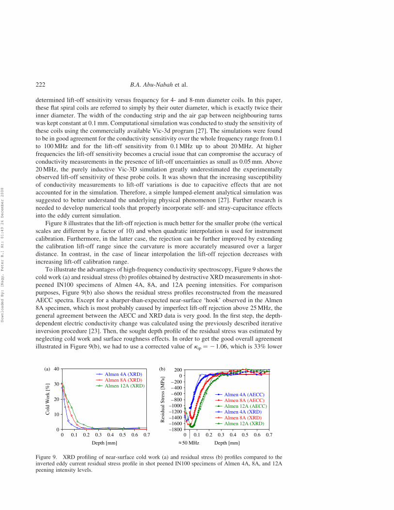
To illustrate the advantages of high-frequency conductivity spectroscopy, Figure 9 shows the

cold work (a) and residual stress (b) profiles obtained by destructive XRDmeasurements in shot-

peened IN100 specimens of Almen 4A, 8A, and 12A peening intensities. For comparison

purposes, Figure 9(b) also shows the residual stress profiles reconstructed from the measured

AECC spectra. Except for a sharper-than-expected near-surface ‘hook’ observed in the Almen

8A specimen, which is most probably caused by imperfect lift-off rejection above 25MHz, the

general agreement between the AECC and XRD data is very good. In the first step, the depth-

dependent electric conductivity change was calculated using the previously described iterative

inversion procedure [23]. Then, the sought depth profile of the residual stress was estimated by

neglecting cold work and surface roughness effects. In order to get the good overall agreement

illustrated in Figure 9(b), we had to use a corrected value of kip ¼ 21.06, which is 33% lower

Figure 9. XRD profiling of near-surface cold work (a) and residual stress (b) profiles compared to theinverted eddy current residual stress profile in shot peened IN100 specimens of Almen 4A, 8A, and 12Apeening intensity levels.



than the independently measured average value for IN100. The exact reason for the need for this

‘empirical’ correction is currently not known and will require further investigation. However, it

should be pointed out that the present underestimation of the residual stress level by the inverted

AECC relative to the destructive XRD results does not seem to be physically related to the above

described overestimation in Waspaloy and IN718 alloys due to increasing electric conductivity

caused by microstructural changes under extensive cold work. Since a single constant was

sufficient to bring all the AECC and XRD results into good agreement with each other for all

three peening intensities in spite of their different levels of cold work, the cause of this apparent

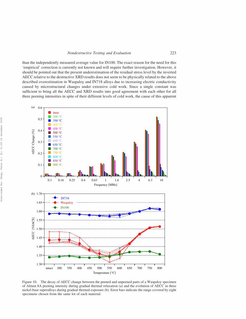
Figure 10. The decay of AECC change between the peened and unpeened parts of a Waspaloy specimenof Almen 8A peening intensity during gradual thermal relaxation (a) and the evolution of AECC in threenickel-base superalloys during gradual thermal exposure (b). Error bars indicate the range covered by eightspecimens chosen from the same lot of each material.



underestimation by the AECC method is most probably the intrinsic variation of the

electroelastic with microstructure.

4. Materials limitations

Previous experimental observations indicated that the sensitivity of eddy current conductivity

spectroscopy is fairly low, but still sufficient for residual stress profiling in certain surface-treated

engine alloys. However, the electrical conductivity and its stress-dependence are rather sensitive to

microstructural variations, therefore the selectivity of this method leaves much to be desired.

Recent research revealed a series of situations where anomalous stress-dependence and relaxation

behaviour were observed. This is not surprising at all in the case of an inherently indirect non

destructive method and should not lead to abandoning the eddy current approach, especially since

no better alternative is known at this point. This chapter reviews four previously unreported recent

experimental observations of anomalous materials behaviour and proposes further research efforts

to better understand the underlying physical mechanisms and to mitigate the adverse influence of

these phenomena on eddy current residual stress profiling.

4.1 Anomalous relaxation in Waspaloy

One of the main questions concerning the feasibility of eddy current residual stress profiling is

whether the AECC difference decays gradually with thermal relaxation or not, which is

extremely important from the point of view of assessing partial relaxation. Initial experimental

evidence indicated that the decay is usually monotonic and gradual, but it was noticed early on

that occasionally the rate of decay was much faster than expected. For example, in one of the first

such experiments aWaspaloy specimen of Almen 8A peening intensity was gradually relaxed by

repeated heat treatments of 24 h each at increasing temperatures in 508C steps from 300 to 9008C

in a protective nitrogen environment [19]. Figure 10(a) shows the observed AECC difference

between the peened and unpeened parts after each heat treatment. These results clearly indicate

that the measured AECC difference gradually decreases during thermal relaxation and almost

completely disappears after the 13th 24-h heat treatment at 9008C. However, there was a very

steep drop in the AECC difference at 4508C, which is highly suspicious as the peening-induced

residual stress is certainly more persistent in Waspaloy at such a low temperature.

Subsequent studies investigated the changing electric conductivity of nickel-base superalloys

due to microstructural evolution at elevated temperatures [25]. Figure 10(b) shows the evolution of

the electrical conductivity in these three nickel-base superalloys (IN718, Waspaloy, IN100) during

gradual thermal exposure. By far the strongest initial inhomogeneity among these materials was

observed inWaspaloy. Itwas also noted that the electric conductivity significantly dropped between

400 and 5008C before it started to increase above 5508C. These results suggested that spurious

electric conductivity variations caused by microstructural anomalies in nickel-base superalloys

interfere with eddy current residual stress assessment of subsurface residual stresses. If the

conductivity variationswere entirely volumetric effects, theywould not cause frequency-dependent

changes in the AECC spectrum, therefore they could be distinguished from near-surface residual

stress and cold work effects caused by surface treatment, which, in contrast, are strongly

frequency-dependent. According to the self-referencing method, the average AECC measured at

sufficiently low frequencies (e.g., between 0.1 and 0.3MHz) is subtracted from the absolute AECC

measured at all frequencies, i.e., the conductivity close to the surface is compared to the conductivity

at a sufficiently large depth where the material can be considered intact, i.e., unaffected by surface

treatment.



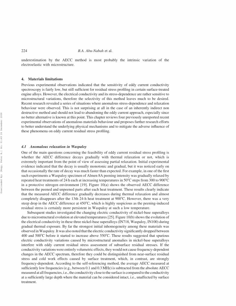
Recent experimental observations indicate that the above assumption is not necessarily valid

in Waspaloy specimens relaxed at around 400–4508C. Figure 11(a) illustrates schematically

how the presence of cold work reduces the transition temperature at which thermally activated

microstructural evolution takes place in the material. For example, let us assume that the

typically 30–40% near-surface plastic strain caused by cold work reduces the activation

temperature by about 408C. If then the surface-treated component is exposed to moderate

temperatures so that the transition occurs in the cold-worked near-surface layer, but not deeper

below the surface, a significant conductivity difference will develop, as it is shown in

Figure 11(b). This effect will be detectable in the measured frequency-dependent AECC

spectrum and could easily overshadow the residual stress relaxation effect that is very weak at

these temperatures. Currently, experiments are underway to verify that the steep drop illustrated

in Figure 10(a) would actually reach below zero if the exposure time were increased. The most

obvious way to mitigate this problem seems to be to expose all the new components to a

carefully chosen heat treatment, e.g., 500–5508C for 24 h. Such treatment would significantly

reduce further changes in conductivity and might not be necessary at all on used components

which tend to develop a uniformly high electric conductivity distribution due to their long

exposure to elevated operational temperatures.

Figure 11. A schematic illustration of how the presence of cold work reduces the transition temperature atwhich thermally activated microstructural evolution takes place in the material (a) and the resulting AECCchange between the cold-worked surface and the intact interior (b).



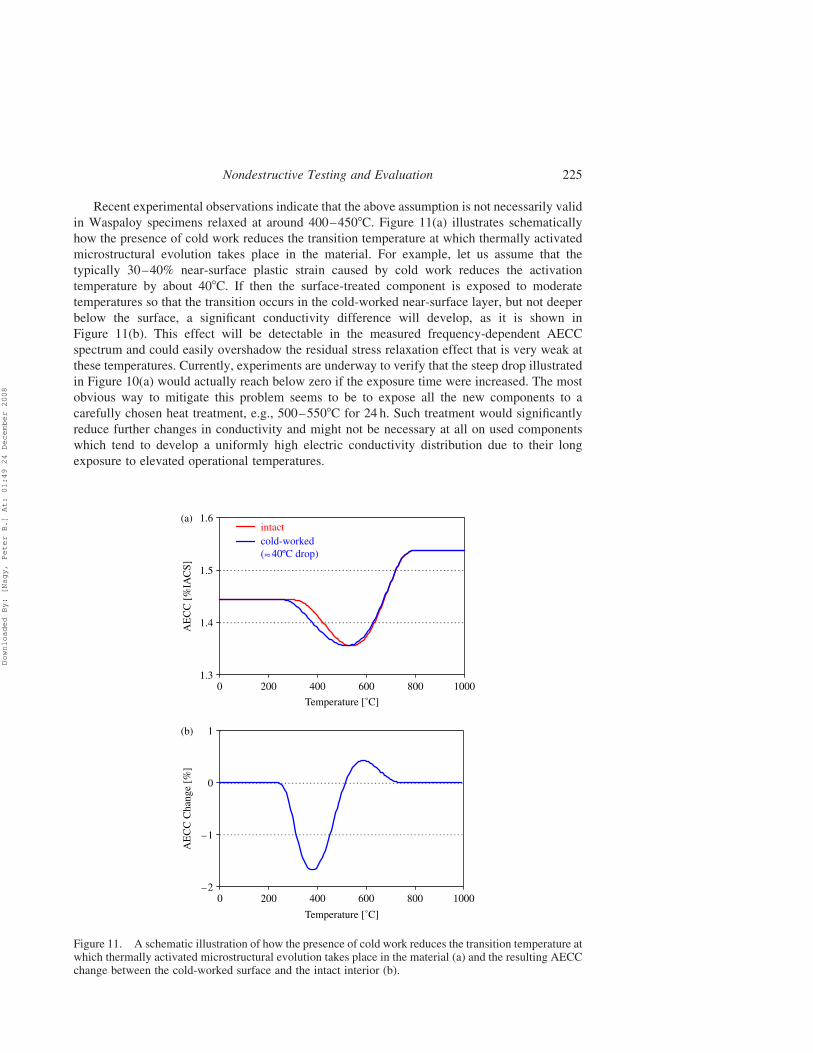
4.2 Anomalous behaviour in hardened IN718

It was recently found that special versions of the common IN718 material can also exhibit

anomalous behaviour that is very different from those of the commercial versions reported in

the literature [19,22,25,28]. A common feature of these materials seems to be that their

custom-designed thermo-mechanical processing results in both increased hardness and

increased electric conductivity. Figure 12 shows examples of AECC spectra measured in

Honeywell Engines DP718 specimens which were shot-peened to Almen 6A intensity and 200%

coverage. The curved specimen (OD ¼ 50.8mm and ID ¼ 34.9mm) shown in Figure 12(a)

was machined from hot rolled material and behaved conventionally, i.e., the AECC increased

with frequency by approximately 1–2%. It should be mentioned that the significant difference

between these spectra above 25MHz indicates uncorrected curvature effects. In comparison, the

AECC spectra measured on the two flat specimens machined from the first batch of forged

material exhibit a much smaller increase in conductivity at high frequencies, which is not

compatible with previous measurements on IN718 and the electroelastic coefficient

independently measured on DP718. Although the reason for this discrepancy is not understood

at present, it seems to be related to the microstructural differences between the two materials.

For example, it was reported in the literature before that soft fully annealed Waspaloy produced

a much stronger AECC increase at high frequencies than harder as-forged Waspaloy [25].

Figure 12. Examples of AECC change measured in Honeywell Engines DP718 specimens shot-peened toAlmen 6A intensity. The curved specimen (OD ¼ 50.8mm and ID ¼ 34.9mm) was machined from hotrolled material (a) while the two flat specimens were machined from forged material (b).



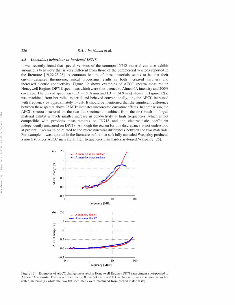
Preliminary results in DP718 indicate that the AECC spectrum is much more variable from

batch to batch than in ordinary IN718 and it exhibits very strange non-monotonic thermal

relaxation behaviour, most probably because of presently poorly understood thermally activated

microstructural evolution. Four flat DP718 specimens of Almen 6A peening intensity and 200%

coverage were prepared for this part of the study by Honeywell Engines from a second batch of

forged material. Subsequently, the peak residual stress in three of these specimens was reduced

to 75, 50, and 25% of the original as-peened level using well-controlled thermal relaxation.

Subsequently, four AECC measurements were conducted at different spots on each specimen

and the results were averaged. Figure 13 shows the AECC change as a function of frequency for

these four specimens. No unique trend can be identified from these results that would correlate

the measured AECC change to the residual stress profiles obtained by XRD. In addition, the

AECC change produced in the second batch of forged DP718 peened under the same nominal

conditions was much less than in the unexpectedly small but still detectable AECC increase

observed in the first batch. The results shown in Figure 13 are very surprising and not properly

understood. Further research is needed to understand why DP718 specimens prepared from

forged stock seem to behave so differently from other nickel-base superalloys tested in earlier

Figure 13. AECC change versus frequency measured in a second batch of flat forged DP718 specimens ofAlmen 6A peening intensity and 200% coverage after thermal relaxation resulting in different relativelevels of retained peak residual stress.

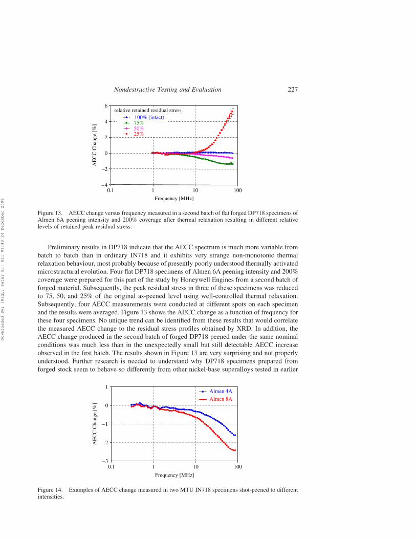
Figure 14. Examples of AECC change measured in two MTU IN718 specimens shot-peened to differentintensities.



studies, when a monotonic correlation between the XRD and AECC results was found. At this

point, the only potentially significant difference we found between DP718 and ordinary IN718 is

the perceivably higher electric conductivity <1.64% IACS of the former versus 1.38–1.56%

IACS for the latter. The parallel and normal electroelastic coefficients of DP718 were

determined following the earlier developed procedure [21]. Based on these measurements we

found that the isotropic plane stress electroelastic coefficient of DP718 is kip < 2 1.22, fairly

similar to the kip < 2 1.54 average value found for IN718, which also excludes the possibility

that the observed anomalous behaviour is residual stress related.

Interestingly, a similar, and probably related, effect was observed recently in custom-treated

IN718 provided by MTU of Munich, Germany. Figure 14 shows the AECC spectra measured in

two MTU IN718 specimens shot-peened to different intensities. These results represent the very

first observation of negative rather than positive AECC change in any as-peened nickel-base

superalloy. The specific microstructural differences between the MTU version of IN718 and

other commercially available versions are presently not known except that the former exhibits

perceivably higher electric conductivity <1.58–1.63% IACS versus 1.38–1.56% IACS and

also significantly higher Vickers hardness around 460HV versus 260HV for commercial IN718

(Hillmann, S. and Meyendorf, N., Private Communication, 2008). The role of different

thermo-mechanical processing on the AECC signature of surface-treated components

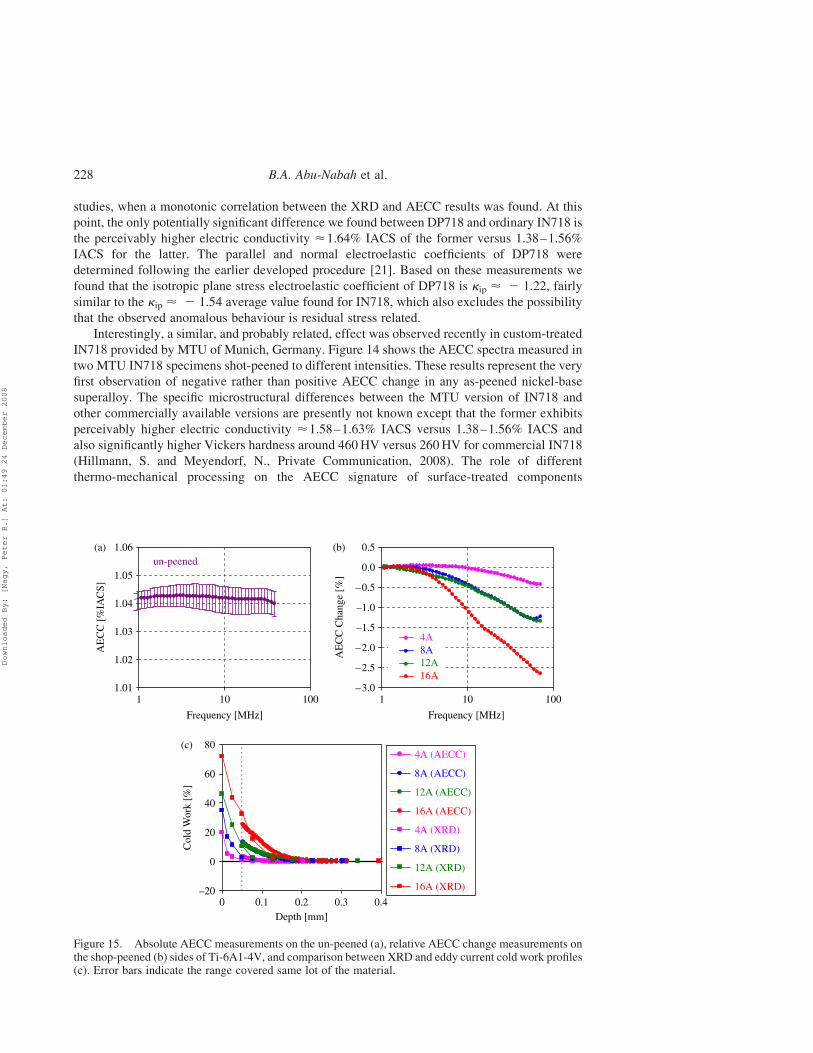
Figure 15. Absolute AECC measurements on the un-peened (a), relative AECC change measurements onthe shop-peened (b) sides of Ti-6A1-4V, and comparison between XRD and eddy current cold work profiles(c). Error bars indicate the range covered same lot of the material.



is currently being investigated at the Fraunhofer Institute for NDT in Dresden, Germany, and the

findings of that study will be published later.

4.3 Profiling in surface-treated Ti–6Al–4V

Initially, Ti–6Al–4V was one of the first materials tested for eddy current residual stress 20

characterisation [11,14]. However, later this interest faded away when it was found that in

Ti–6Al–4V the electric conductivity is insensitive to isotropic plane stress, as it was illustrated

in Figure 2. Because of direct exposure to erosion and foreign body impact damage, NDE of

low-temperature inlet fan and compressor blades, which are usually made of titanium alloys, is

even more important than that of high-temperature turbine components downstream, which are

usually made of nickel-base superalloys. Therefore, reliable engine rotor life prognostics

absolutely requires that an eddy current, or other suitable NDE method be developed for near-

surface cold work characterisation in titanium alloy components.

One of the main reasons why titanium alloys were originally thought to be less promising

candidates for eddy current inspection is that they dominantly crystallise in hexagonal symmetry

and therefore exhibit significant texture-induced electric anisotropy on the order of 3–4%

relative conductivity variation in a highly textured Ti–6Al–4V plate [39]. Our initial

measurements on shot-peened Ti–6Al–4V indicated a decrease in apparent eddy conductivity

near the surface [19]. Since the stress-dependence of electric conductivity is almost negligible in

Ti–6Al–4V and the surface roughness induced AECC loss is also negligible below 20MHz, it

was recently suggested that eddy current conductivity spectroscopy is selectively sensitive to

crystallographic and morphological texture in the shot-peened Ti–6Al–4V and it might be

exploited for near-surface cold work profiling [43].

Figure 15(a) shows the average of AECC measurements taken on the un-peened sides of four

Ti–6Al–4V specimens. In spite of the significant point-to-point variation of conductivity, these

results indicate that the average base-line conductivity spectrum is essentially frequency-

independent up to 40MHz, which illustrates that spatial averaging can sufficiently reduce the

adverse inhomogeneity effect on AECC measurements. For this reason, spatial averaging was

conducted on the peened sides as well. Figure 15(b) illustrates the average AECC changemeasured

at four locations clustered around the centre on the peened side of four specimens peened at four

different intensities. These results indicate that increasing the peening intensity level increases the

drop inAECCmeasurementswith frequency.However, there is a virtual overlapbetween theAECC

change of the Almen 8A and 12A specimens. To check the reproducibility of these results, other

specimens of Almen 8A and 12A from the same batch were tested and the results were found to be

consistent in terms of AECC change even though they correspond to slightly different near-surface

residual stress and cold work profiles.

Since near-surface cold work is the dominant factor affecting the AECC change in

shot-peened Ti–6Al–4V, the AECC change can be correlated to the presence of cold work alone

through an empirically determined dimensionless isotropic plane electroplastic coefficient [43].

Figure 15(c) shows a comparison between XRD and eddy current cold work profiles.

The frequency-dependent AECC change was first inverted to a depth-dependent electric

conductivity profile using the simplistic inversion technique [20]. Then, the depth-dependent

conductivity change was converted into the near-surface cold work profile assuming a

dimensionless isotropic plane electroplastic coefficient of 20.08 which was determined by best

fitting of the inverted eddy current results to the near-surface cold work profiles obtained by

destructive XRDmeasurements. The recently developed iterative inversion technique could not be

used due the sharp change in the depth-dependent conductivity profile within a short distance

below the surface [23]. However, the results using the more robust simplistic inversion technique



indicate the possibility of using AECC measurements for near-surface cold work profiling in shot-

peened Ti–6Al–4V.

5. Conclusions

This paper dealt with nondestructive characterisation of near-surface residual stress caused by

plastic deformation during surface treatment. Residual stress causes remnant elastic strain,

i.e., change in lattice separation, even in the absence of external applied loads. Surface

treatments aim at producing compressive subsurface residual stresses that can significantly

extend the fatigue life of fracture–critical components. Depending on how the plastic

deformation was achieved by cold work, e.g., by SP, LSP, or LPB, surface treatment also

leaves substantial microstructural damage behind in the material. The degree of cold work is

often characterised simply by the amount of plastic strain produced in the material. Although

cold work might have some beneficial effects on the material, such as surface hardening, in

most cases it affects adversely the material. In particular, cold-work-induced microstructural

damage is largely responsible for the accelerated thermal relaxation of protective residual

stress in surface-treated components. In most engine materials, this adverse effect of cold

work becomes especially strong above 10% equivalent plastic strain, which is why SP, that

produces as much as 20–40% plastic strain at the surface, is so inefficient on critical

components operating at elevated temperatures. The potential of thermal relaxation at elevated

operational temperatures necessitates repeated checks during periodic maintenance. Since,

existing inspection methods either cannot be applied to subsurface residual stress assessment

or are destructive in nature, new nondestructive characterisation methods are being sought to

replace them. Eddy current conductivity spectroscopy has emerged as one of the leading

candidates for non-destructive residual stress profiling in surface-treated metals. This is an

experimental method that will require further research before it can be applied in field

inspection. Currently, its feasibility for quality monitoring during manufacturing and assessing

subsequent relaxation during service has been demonstrated only for certain nickel-base

superalloys. The main limitation of residual stress profiling by eddy current conductivity

spectroscopy is that, although the method is sensitive enough to weak elastic strains to be

practically useful, it is not sufficiently selective for them. Even for the limited range of

nickel-base superalloys numerous limitations have been identified in the literature, such as

spurious inhomogeneity in some forged engine alloys, interference from cold-work-induced

microstructural damage, and practical inspection difficulties associated with the very high

inspection frequencies required to capture the peak compressive stress in moderately

shot-peened components. Because of the aforementioned limitations, eddy current

conductivity spectroscopy cannot be expected to replace XRD residual stress measurements.

However, because of its relative simplicity and nondestructive nature, it might supplement

this more accurate but destructive XRD technique.

This paper discussed numerous recently discovered additional materials limitations that are

presently not properly understood. The presented experimental evidence indicates that the

excess AECC in surface-treated nickel-base superalloys is due in part to elastic strains, i.e.,

residual stress, and in part to plastic strains, i.e., cold work, and it is also adversely influenced by

thermally or thermo-mechanically activated microstructural changes. The very fact that the

conductivity increases rather than decreases was originally thought to indicate that the observed

AECC increase was mainly due to the presence of compressive residual stresses. This

assumption was also supported by XRD results on fully relaxed specimens showing that the cold

work induced widening of the diffraction beam only partially vanishes when both the residual

stress and the AECC completely disappear due to thermal relaxation.



Phase transformations can occur in nickel-base superalloys parallel to residual stress

relaxation at normal operational temperatures of engine components. There is mounting

evidence that in the presence of plastic deformation damage thermal exposure can lead to

accelerated microstructure evolution which causes conductivity changes that interfere with, and

sometimes even overshadow, direct indications of the residual stress and cold work effects

caused directly by the surface treatment. Experimental observations first reported in this paper

indicate that some of these crucial materials issues have not been solved sufficiently for this

technique to be adopted for field applications yet and further research is needed to better

understand the underlying physical phenomena and the influence of materials variations.

Although we did not measure the chemical composition of our nickel-base superalloy

specimens, they all complied with tight tolerances specified for such engine materials. Based on

our most recent observations, referring to these materials by their commercial name and general

thermomechanical processing (fully annealed, hot rolled, forged, precipitation hardened, etc.)

might not be sufficient for the purposes of understanding the specific behaviour exhibited by

these materials. One of the main goals of this paper was to draw attention to the need for further

research of the unresolved materials issues. Specifically, additional research is needed to better

understand the correlation between hardness and electroelastic/electroplastic behaviour in these

materials.

Acknowledgments

This work was supported by the Air Force Research Laboratory partly under Contract No. F33615-03-2-5210 with the University of Cincinnati and partly through the Quantitative Inspection Technology forAging Military Aircraft program with Iowa State University on delivery order number 5007-IOWA-001 ofthe prime contract F09650-00-D-0018. Additional support was provided through cooperation with theCenter for NDE at Iowa State University with funding from the Air Force Research Laboratory on contractFA 8650-04-C-5228. The diffraction measurements reported in this study were made by Lambda Researchof Cincinnati. The authors would like to acknowledge valuable discussions and ongoing collaboration withSusanne Hillmann and Norbert Meyendorf of the Fraunhofer Institute for NDT in Dresden, Germany.

Notes

1. General Electric Aviation, Cincinnati, OH 45215, USA.2. Cessna Aircraft, Wichita, KS 67277, USA.3. Rolls-Royce Corporation, Indianapolis, IN 46241, USA.

References

[1] V. Hauk, Structural and Residual Stress Analysis by Nondestructive Methods, Elsevier, Amsterdam,Netherlands, 1997.

[2] J.T. Cammett, P.S. Prevey, and N. Jayaraman, Proceedings of ICSP 9, Marne-la-Vallee, Paris, France,2005.

[3] P.S. Prevey, IITT-International, Gournay-Sur-Marne, France (1990), p. 81.[4] D.J. Hornbach, P.S. Prevey, and M. Blodgett, Review of Progress in Quantitative NDE, Vol. 24,

American Institute of Physics, Melville, NY, 2005, pp. 1379–1386.[5] M.G. Moore and W.P. Evans, Mathematical Correction for Stress in Removal Layers in X-ray

Diffraction Residual Stress Analysis. SAE Trans. 66 (1958), pp. 340–345.[6] M. Francois, F. Convert, and J. Lu, ‘X-Ray Diffraction Method’ Handbook of Measurement of

Residual Stresses, Society of Experimental Mechanics, Fairmont Press, Lilburn, GA, 1996,pp. 71–132.

[7] G. Maeder, M. Barral, J.L. Lebrun, and J.M. Sprauel, Rigaku J. 3 (1986), pp. 9–21.[8] A. Pyzalla, J. Nondestr. Eval. 19 (2000), pp. 21–31.



[9] N. Goldfine, 41st Army Sagamore Conference, Plymouth, MA, 1994.[10] N. Goldfine, D. Clark, and T. Lovett, EPRI Topical Workshop: Electromagnetic NDE Applications in

the Electric Power Industry, Charlotte, NC, 1995.[11] F.C. Jr. Schoenig, J.A. Soules, H. Chang, and J.J. DiCillo, Mater. Eval. 53 (1995), pp. 22–26.[12] M. Blaszkiewicz, L. Albertin, and W. Junker, Mater. Sci. Forum 210 (1996), pp. 179–186.[13] N. Goldfine and D. Clark, EPRI Balance of plant heat exchanger NDE Symposium, Jackson, WY,

1996.[14] H. Chang, F.C. Jr. Schoenig, and J.A. Soules, Mater. Eval. 57 (1999), pp. 1257–1260.[15] I. Lavrentyev, P.A. Stucky, and W.A. Veronesi, Review of Progress in Quantitative NDE, Vol. 19,

American Institute of Physics, Melville, NY, 2000, pp. 1621–1628.[16] J.M. Fisher, N. Goldfine, and N. Zilberstein, 49th Defense Working Group on NDT, Biloxy, MS, 2000.[17] V. Zilberstein, Y. Sheiretov, A. Washabaugh, Y. Chen, and N. Goldfine, Review of Progress in

Quantitative NDE, Vol. 20, American Institute of Physics, Melville, NY, 2001, pp. 985–995.[18] V. Zilberstein, M. Fisher, D. Grundy, D. Schlicker, V. Tsukernik, V. Vengrinovich, N. Goldfine, and

T. Yentzer, J. ASME, Pressure Vessel Technol. 124 (2002), pp. 375–381.[19] M.P. Blodgett and P.B. Nagy, J. Nondestr. Eval. 23 (2004), pp. 107–123.[20] F. Yu and P.B. Nagy, J. Appl. Phys. 96 (2004a), pp. 1257–1266.[21] ———, J. Nondestr. Eval. 24 (2005), pp. 143–152.[22] ———, J. Nondestr. Eval. 25 (2006), pp. 107–122.[23] B.A. Abu-Nabah and P.B. Nagy, NDT&E Int. 39 (2006), pp. 641–651.[24] N. Nakagawa, C. Lee, and Y. Shen, Review of Progress in Quantitative NDE, Vol. 25, American

Institute of Physics, Melville, NY, 2006, pp. 14718–1425.[25] F. Yu, M.P. Blodgett, and P.B. Nagy, J. Nondestr. Eval. 25 (2006), pp. 17–28.[26] B.A. Abu-Nabah and P.B. Nagy, NDT&E Int. 40 (2007a), pp. 405–418.[27] ———, NDT&E Int. 40 (2007b), pp. 555–565.[28] Y. Shen, C. Lee, C.C. H. Lo, N. Nakagawa, and A.M. Frishman, J. Appl. Phys. 101 (2007), p. 014907.[29] M.P. Blodgett, C.V. Ukpabi, and P.B. Nagy, Mater. Eval. 61 (2003), pp. 765–772.[30] K. Kalyanasundaram and P.B. Nagy, NDT&E Int. 37 (2004), pp. 47–56.[31] F. Yu and P.B. Nagy, J. Appl. Phys. 95 (2004b), pp. 8340–8351.[32] C.S. Smith, Solid State Physics, Advance in Research and Application, Vol. 6, Academic, New York,

NY, 1958, pp. 175–249.[33] M. Bao and Y. Huang, J. Micromech. Microeng. 14 (2004), pp. 332–334.[34] E. Barsis, E. Williams, and C. Skoog, J. Appl. Phys. 41 (1970), pp. 5155–5162.[35] Z. Rosenberg, D. Yaziv, and Y. Partom, J. Appl. Phys. 51 (1980), pp. 4790–4798.[36] Y. Partom, D. Yaziv, and Z. Rosenberg, J. Appl. Phys. 52 (1981), pp. 4610–4616.[37] D.Y. Chen, Y.M. Gupta, and M.H. Miles, J. Appl. Phys. 55 (1984), pp. 3984–3993.[38] Y. Partom, Z. Rosenberg, and B. Keren, J. Appl. Phys. 56 (1984), pp. 552–553.[39] M.P. Blodgett and P.B. Nagy, Appl. Phys. Lett. 72 (1998), pp. 1045–1047.[40] N.J. Goldfine, Mat. Eval. 51 (1993), pp. 396–405.[41] R.J. Ditchburn, S.K. Burke, and M. Posada, J. Nondestr. Eval. 22 (2003), pp. 63–77.[42] R.J. Ditchburn and S.K. Burke, NDT&E Int. 38 (2005), pp. 690–700.[43] B.A. Abu-Nabah and P.B. Nagy, Review of Progress in Quantative NDE, Vol. 27, American Institute

of Physics, Melville, NY, 2008, 1228–1235.



Documents

Eddy current residual stress proﬁling in surface-treated ...pnagy/publications/Abu-Nabah et al., Nondestr. Test... · Eddy current residual stress proﬁling in surface-treated