EDEA- An Expert Knowledge-Based Tool for Performance Measurement

Kamel Bala

A thesis submitted to the Faculty of Graduate Studies in partial fulfillment of the requirernents

for the degree of

Doctor of Philosophy

Schulich School of Business York University

Toronto, ON, M6J 1P3

August 23,2001

National Library I*I ofCanada Bibliothèque nationde du Canada

Acquisitions and Acquisitions et Bibliographie Services services bibliographiques

395 Wellington Street 395. rue Wellington Ottawa ON K1A O N 4 OüawaON K I A W Canada Canada

The author has granted a non- exclusive licence allowing the NationaI Libmy of Canada to reproduce, loan, distribute or seU copies of this thesis in microfonn, paper or electronic formats.

The author retains ownership of the copyright in this thesis. Neither the thesis nor substantial extracts fiom it may be printed or othenvise reproduced without the author's permission.

L'auteur a accordé une licence non exclusive permettant à la Bibliothèque nationale du Canada de reproduire, prêter, disbcibuer ou vendre des copies de cette thèse sous la forme de microfiche/film, de reproduction sur papier ou sur format électronique.

L'auteur conserve la propriété du droit d'auteur qui protège cette thèse. Ni la thèse ni des extraits substantiels de celle-ci ne doivent être imprimés ou autrement reproduits sans son autorisation.

EDEA-AN EXPERT KNOWLEDGE-BASED PERFORMANCE MEASUREMENT TOOL

a dissertation submitted to the Faculty of Graduate Studies of York University in partial fulfillment of the requirements for the degree of

OOCTOR OF PHILOSOPHY

O Permission has been granted to the LIBRARY OF YORK UNIVERSITY to lend or sel1 copies of this dissertation. to the NATIONAL LIBRARY OF CANADA to microfilm this dissertation and to lend or seIl copies of the film, and to UNIVERSITY MlCROFlLMS to publish an abstract of this dissertation. The author reserves other publication rights, and neither the dissertation nor extensive extracts from it may be printed or otherwise reproduced without the author's writtefl permission.

ABSTRACT

This thesis presents an irnproved measurement tool for evaluating performance of

branches within a major Canadian bank. While there have been numerous previous

studies of performance at a branch levsl. within the banking industry. this study is

different in a signifîcant ariy: specifically two kinds of data are used to develop the

rnodel .

The first t>*pe of data is standard transaction data a\-ailable frorn an>- b a k . Such data have

formcd the basis of pre\ious studies. The second type of data. obtained from the site

studied. is what can be called classification information. based on branch

consultant/espert judgment as to good or poor performance of branches.

The purpose here is to develop an expert knowledge-based version of an esisting

benchrnarking model. Data Envelopment Analysis (DEA). and to show how this tool is

applied in the banking industr]i*. To reflect this extension of the basic DEA modeI. we

adopt the acronym EDEA.

Chapter 1 presents the contest of the research and briefly describes knowledge

acquisition techniques.

Chaptsr 2 introduces the DE.4 theor'.. ~vith its major modsls. and describes three diffèrent

discriminant techniques. namely:

Logistic regrsssion. nhich is based on the Maximum Likelihood concept:

Discriminant analysis. based on centroids and groups:

Goal programming. a powerful extension of linear prograrnming.

Chaptsr 3 builds classification concepts into the additive DEA model. It demonstrates

how DEA measures can be enhanced. by incorporating expert judgement into the

structure. This enhancement facilitates variable selection. as part of the modeling

esercise. This new mrthodology is tested using a set of data provided by a major

Canadian bank.

Chapter 4 estends the ideas of Chapter 3 to a nonlinear (input-orienred) DEA model

structure. As well. this chapter extends the expert system structure. by adding further

knowlsdge information in the form of a specification of the status (output or input). of a

subset o f the variables.

Chapter 5 investigates a number of extensions o f the models of the two previous chapters.

Specifically. an investigation is performed regarding the imposition of certain constraints

into the earlier models.

Conclusions are presented in Chapter 6.

ACKNOWLEDGEMENTS

1 would like to thank several people who have significantly contributed to this thesis.

In particular 1 am indebted to my supervisor. Professor Wade D. Cook (Mana, oement

Science). who proved to be an effective and unmatchable mentor.

1 u-ould also like to thank committee members Professor Gordon Roberts (Finance).

Professor Scott l'eomans (Management Science). and Professor Markus BiehI

(Management Science).

1 am also graieful to Dr. Mosz Hababou for his invaluable help and advice.

Finall!.. 1 would like to thanli m y family who helped and supported me. and who have

made this effort worthwhile.

TABLE OF CONTENTS

I I . OVERVIEW O F PERFORMANCE MEASUREMENT MODELS AND CLASSIFICATION TOOLS ......................................................................................................................................................... 1 1

I I . 1 DATA ESVELOPXIEST AS.-\LI'SIS MODEM .................................................................................... 1 1 1 . . I The concept ............................................................................................................................ / l 1 . 2 DE.?.\f~di.l~. . . . . . . . . . . . . . . . . . . . . . . . . . . . . . . . . . . . . . . . . . . . . . . . . . . . . . . . . . . . . . . . . . . . . . . . . . . . . . . . . . . . . . . . . . . . . . . . . . . . . . . I - f

.............................................................................................. 1 . 3 Mujor DE.4 . \ /UC/C/ Euerisiom -24 1 . 1.4 Srrengths und L~tnirurions ofDE.4 ......................................................................................... 23

1 . 2 DISCRlMIKAST MODELS ............................................................................................................. 27 7- 11.2. / Logisric Regwssiot~ ............................................................................................................... .-

............................................................................................. . I I 2.2 Multiple Disc*rin~ri~artr ? nui\-sis 32 1 . 2 3 Lirwar Gocd Pt-ugraniniit7g DiscritnNianr hfodels .................................................................. 37

III . EMBEDDING EXPERT KNOWLEDGE IN T H E ADDITIVE DEA MODEL ........................ 35

1 11 . 1 1 NTRODCCTIO'I ............................................................................................................................. .A4 /// . 1 / Linkirig disct-iturrtarir tecituiqms und the .-Iddiri i.e DE.4 Mo&/ ........................................... 50 /// . / 2 Daru Trat~fort t~~rt~oti ............................................................................................................ 33 I l 1 DE.4 .\le~r.swc.s .................................................................................................................... 55

111.2 METHODOLOGY .............................................................................................................................. 58 111.3 ESPERIMEST L!SIXG AS . ADDITIL'E DEA MODEL ............................................................................ 61

............................................................................................ / . . I Estinlaring rite Predictire . \focid 61 111.3 7 T e s h g tlw Pr~"it i tr i -~ . \ fo~/cl . . . . . . . . . . . . . . . . . . . . . . . . . . . . . . . . . . . . . . . . . . . . . . . . . . . . . . . . . . . . . . . . . . . . . . . . . -1

1 ' . EMBEDDING EXPERT KNOWLEDGE IN THE INPUT-ORIENTED DEA MODEL ......... 78

IV . I ISTRODUCTIOS ............................................................................................................................... 78 IV.? ESPERIMEST trS1sc; AS ISPCT-ORIENTED DEA MODEL ................................................................ 79

1 . 2 . / Estitmti17y rlir Pt-dicri)-e . t fodrl ..................................................................................... ' 9 ............................................................................. I 2 . 2 Tesfing rli t. Pt.èJicrrt.t, .\fodcl ............. .... 83

IV.3 COSCLUS [os ........................................................ .. ..................................................................... 85 / 3 1 C/ass1ficatioi7 uf'lio/~/ou/ surrrplrs ......................................................................................... 8- 11.. 3.2 Cases ~-itlr prt'tl@ed Iripzrr attd Ourpzrr variables ................................................................ 8 9

V . MODEL EXTENSIONS ..................................................................................................................... 99

...................................................... V . 1 DEA MODEL EXlIASCE31EST- EXPERT OP~N~OS CONSTRAINTS 99 I .. 1.1 imposir~g Goal Progranrn~irig Consrraints wirhin an -4 dditivr DE.? Mode1 ........................... 99

I . 2 Iniposrrtg Goal Pt-ogratnntitlg Co)tstraints ro an lnpzrl Orienred DEA Mode/ ..................... / O 8 V.2 EXTENSION TO X1ORE THAN T\V0 CLASSES .................................................................................. 119 V.3 SENSITIVITY As.-\L\.sIs ................................................................................................................ 135

VI . CONCLUSION .............................................................................................................................. 127

VI1 . APPENDIX .................................................................................................................................... 131

vii

...................................................... .................. 1 7 . 1 . 2 Facror atzalr.sis rs Componen r ana!vsis .. 133 .................................................................................. 1 3 Facror .-lna -.sis Decision Diagrant 133

........................................................................................................ 1 . 1.4 The rorarion of Facrors 133 7 1.5 Crireria for rhe "Vzrmber of Facrors ro Be Extracred ......................................................... 137

................................................................. 1'11 . 1.6 Crireriafor rhe sigruficance of Facror Loadings 139 ........................................................................................................................... . ' 1 1. 7 L imiraliom 140

.............................................................. ' 1 1 1.8 Afarrir Formiilarion ofrhe Factor ..l n a b i s Mode1 141 ................................................................................................. . . 1 . 1 9 Facror .4nalj .sis Kej Termr 1 4 2

........................................................................................ V I 1.2 DATA SET PROViDED B'i' THE BANK 144 V I 1.3 D I S C R I ~ ~ I S :I NT ANALYSK COEFFICIENT RESULTS ..................................................................... 149

TABLE OF FIGURES FIGLiRE 1- 1 . REGRESSIOS LINE VS . FRONTIER LlNE ..................................... ... ................................................. 2 FIGURE 1-2: STANDARD DATA VS . HEURISTICS ............................... ... ......................................................... 7 FIGURE 1-3: KSOWLEDGE ACQUISITION TO I ~ ~ P R O V E DEA MODELS ............................................................ 10 FIGURE 11-1 : A BANK BRANCH CONSUMNG 2 INPUTS TO PRODUCE 2 OLTPL~TS .................................... .... 1 1 FIGURE 11-2 : COMP.ARISOX O F DEA ASD REGRESS!ON AXALYSIS ..................... .. ...................................... 13 FIGURE 11-3 ENVELOPXIENT SURFACE FOR THE ADDITIVE MODEL ......................... .... ............................. 14 FIGURE I I 4 : DEA RATIO AND NET PROFIT ORIENTED MODELS ..................... .. ....................................... 15 FIGURE 11-5 : DEA MODEL ORIENTATION ......................... .. ...................................................................... 16 FIGURE 11-6 : ESVELOP~IENT SURFACE FOR THE ADDITIVE MODEL ............................................................. 17 FIGURE 11-7 : ENVELOPMENT SURFACE FOR THE CCR-1 MODEL (CRS) ....................................................... 19 FIGURE 11-8 : ENVELOPXIEST SURFACE FOR THE CCR-O MODEL (CRS) ...................................................... 19 FIGGRE 11-9 : RATIO VS LISEAR DEA FOR.VCLATIOYS ................................................................................. 23 FIGURE 11-1 0: MODEL CL.ASSIFICATIOS BASED OS THE DISTRIBLITIOX OF T H E R-\SDOM COMPONENT ..... 2 8 FIGURE 11-1 1 : LOGIT RESPONSE FL~SCTION ................................................................................................... 30 - - FIGURE 11- 13 : DISCRIXIIN.ANT ANALYSIS CENTROIDS ................................................................................... 23 -. FIGURE Il-l3 : MDA RC'LE ............................................................................................................................ 23

FIGURE I I - I 4 : MD.4 OVERL.VPISG DIsTRIBUTIO.\;S ..................................................................................... 34 FIGURE 11- 1 5 : MDA OPTI~ILIS! TWRESHOLDS ................................ .. ................................................ ........35 FIGURE I I - 16 : GOAL PROGRX~!~IISG COSSTR.AIST ..................................................................................... ..38 FIGURE I I - I 7 : I[.LCSTR..\TION O F ISTEGER PROGR.A~\I.~~ISG DISCRI\IISANT MODEL ..................................... 41 FIGURE I I - 18 : GOAL P R O G R . . \ S I ~ M CLASSIFICATIOS WTH O\'ERLAPPISG GROCPS .................................. 4 3 FIGCRE I I 1- I : DISCRI%IIS.-\ST TECIISIQLTS VS . DEA ................................................................................. 4 8 FIGL~RE II I - ? PRIYCIPLE O F THE THEORY THAT IMPROVES DEA MODELS ................................................... 49 FIGURE 111-3 : DATA PROJECTIOS .................................................................................................................. 5 5 FIGURE I I I - l : TEK-FOLD CROSS VXL[D.ATIOS MET HO DO LOG'^' .................................................................... 6 0 FIGCRE I I 1-5 : GESER..\L STEPS FOR THE ADDITIVE DEA ESPERIMEST ........................................................ 61 FIGURE 111-6: R=~SDO~I S X X ~ P L I M ~ ST.-\GE ..................................................................................................... 6 2 FIGURE 111-7: DETER%lISISG JKPL'TS ASD 01'11>1:TS FOR SCES.-~RIO = I %'[TH LOGISTIC' REGRESSION (LR) .. 6 3 FIGVRE III-8 : DISCRI\(ISAST TECMSIQL'ES STAGL ....................................................................................... 64 FIGURE 111-9 : D E A CO~IBIN.ATORIAL STAGE (ADDITIVE ESPERI~IEST) ....................................................... 66 FIGURE 111- 10 : MATCHING DEA SCORES STAGE .......................................................................................... 6 8 FIGURE I I 1-1 1 : CLASSIFICATION SLWXIARY TABLE STAGE ........................................................................... 6 9 FIGURE I I I - 12 : DEA PREDICTIVE CLASSIFIC.L\TIOS STAGE ......................... ... ........................................... 72 FIGCRE I I I - 13 : COVPLETE VS PARTIAL DEA ANALYSES ............................................................................. 7 3 FIGURE 111- 14 : DEA PREDICTIVE STAGE ...................................................................................................... 74 FIGL'RE I I 1- 15 : MATCI~IXG DEA SCORES STAGE .......................................................................................... 7 5 FIGURE 111-1 6 : C L ~ ~ I F I C A T I O K SLNMARY TABLE STAGE .......................................................................... 76 FIGURE IV-1 : GENERAL STEPS FOR THE INPUT DE.4 EXPERIMENT ................... .. ...... .. ........................... 80 FIGURE IV-?: ILLUSTRATION OF ~ N K I N G DEA RESULTS (ADDITIVE MODEL/AN.ALYSIS STAGE) ............... 86

............ FIGCRE IV-3: ILLUSTRATION O F RANKING DEA RESULTS (ADDITIVE MODEL/PREDICTIVE STAGE) 8 7 FIGURE 1V-4: RESTRICTING WEIGHTS OF G 0 . 4 ~ P R O G ~ M N G MODEL ...................................................... 9 2 FIGURE V- 1 : IMPOSING GOAL P R O G R A M ~ ~ G CONSTRAINTS ON A DEA MODEL ...................................... 100 FIGURE V-2 - RESTRICTEO VS . UNRESTRICTED ADDITIVE DEA MODEL ..................................................... 105 FIGURE V-3: NON-RESTRICTED ADDITIVE DEA MODEL ............................................................................. 107 FIGURE V-4: RESTRICTED ADDITIVE DEA MODEL = 1 ................................................................................. 108 FIGURE V-5: NON-RESTRICTED INPUT DEA MODEL ................................................................................... 1 13 FIGURE V-6: RESTRICTED INPUT DEA MODEL f: l (NON LINEAR CONSTRAIKTS) ........................................ 1 14 FIGURE V-7: RESTRICTED INPUT DEA MODEL # 1 (LINEAR CONSTRAINTS) ................................................ 1 17 FIGURE V-8: IMPOSING GOAL P R O G R . ~ MMIKG CONSTRAINTS ON A DEA MODEL (3 GROL'PS) .................. 1 19 F I G U R E VI-I : DEA LEARNING MODEL .................................................................................................... 1 2 9

LIST OF TABLES TABLE 111- 1 : DEA VARIABLES ..................................................................................................................... 50 TABLE I I I - ? : LOGISTIC REGRESSION SAMPLE RESCLTS ....................... .,. ........ ... ................................... 64 T ~ L E 111-3 : DEA CLASSIFICATION TABLE FOR SCENARIO 2 I (OUT O F 1 O) .................. .... ..................... 67 TABLE I I 1 3 : DEA CLASSIFICATION TABLE FOR THE LOGISTIC REGRESSION ............................................... 69 TABLE I I 1-5 : SLMX~ARIZED DEA CLASSIFICATION T ~ L E (ADDITI'JE MODE~J'ANALYSIS STAGE) ............... 71 TABLE 111-6 : S U ~ ~ ~ ~ A R I Z E D DEA CLASSIFICATION TULE (ADDITIVE MODEL~PREDICTIVE STAGE) ............ 77 TABLE IV- 1 : DEA CLASSIFICATION TABLE FOR SCENARIO :: 1 (OUT O F IO) ................................................ 81 TABLE IV-? : DEA CLASSIFICATION TABLE FOR T H E LOGISTIC REGRESSION .............................................. 82

............ TMLE IV-:: SUMM.~RIZED DEA CLASSIFICATION T . ~ L E (INPUT DEA MODEL/AN.ALYSIS STAGE) 83 .......... TABLE IV-4: SCMXIARIZED DEA CLASSIFICATIOX T M L E (INPCT DEA MODEL'PREDICTIVE ST .GE) 84

TABLE IV-5: COMPARISON OF ANALYSIS STAGE RESULTS ......................................................................... 85 TABLE IV-6: COW.-\RISOS OF PREDICTIVE STAGE RESC~LTS ........................................................................ 86 TABLE IV-7 : CL ..\ SSIFICXTIOS OF HOLDOUT SAMPLES U s r w ADDITIVE DEA MODEM AXD G 0 . 4 ~

PROGR..\II\IISG COEFFICIENT SIGNS TO SELECT ISPCTS AKD OUTPCTS ................................................ 89 TABLE IV-S : CL.ASSIFIC~\TIOS OF HOLDOL'T SAMPLES USIXG ~ N P L ~ T DEA MODELS ASD GOAL

................................................ P R O G R W ~ I I X G COEFFICIENT SIGNS TO SELECT INPUTS AND OLITPCTS 89 TABLE IV-9: V . A R I . ~ L E PREDEF~NED ORIENTATIOSS .................................................................................... 90 TABLE IV- IO: ADDITIVE DEA CLASSIFICATIO~ TABLE FOR SCES.MIO 2 I ................................................... 9 4 TABLE IV- l 1 : ISPL'T DEA CLASSIFICATION T.ABLE FOR SCENXRIO I ...................................... T.AB~.E IV- 12: X\XK : \GED ADDITIVE DEA CL.4SS1FiCATIOS RESLILTS FOR THE I O SCES..\RIO~ ................... 97 T..\BLE IV- 15: AL'ERAGED INPCT DEA CLASSIFICATIOS RESLrLTS FOR THE 10 ScEN..\RlOS ......................... 9 8

................................... TABLE V- I : S C ~ I . . \ R I Z E D RESULTS FOR THE ADDITI\'E RESTRICTED ESPERIMENT 106 ......................................... T..\BLE V-2: S L ~ X I A R I Z E D RESULTS FOR THE ISPCT RESTRICTED ESPERIMEKT I 12

TABLE V-3: SLIIXIARIZED RESLLTS FOR THE ISPET RESTRICTED ESPERIMENT (LISEAR COSSTRAIXTS) .. I 16 T:\BLE V-4: SL!\I\I.ARY O F RESTRICTED DEA MODEL ............................................................................... 1 18

... TABLE V-5 : SEYSITIVITY ASALYSIS WlTH INPUT DEA MODELS USKG S.WPLES OF DIFFERENT SIZES 126 TABLE VII- 1 : GOXL PROGR.4iclMING SAMPLE RESCLTS .............................................................................. 149 .T..\si.tl V11-2 : GOXL PROGRAXI.VING SAXIPLE RESC'LTS (N.IT!{ RESC. - \ l .~~ D ..\TA ) ....................................... 1-49 TABLE VI 1-3 : I N T E G E R LISE.^ P R O G U ~ I ~ I I X G S.-\MPLE RESCL'TS ............................................................ 149

...................... TABLE L'Il-4 : ISTEGER LISEAR P R O G R A ~ M ~ ~ G SAS~PLE RESULTS (Ii'lTH RESC..\LED D.AT.4) I 50 ....................................................... TABLE VII-5 : MCLTIPLE DISCRIMINANT AMLI'SIS S.AMPLE RESCLTS 150

1. INTRODUCTION

1.1 PERFORMANCE MEASUREMENT

In todaj.'s business environment, particulariy in financial services, it is a constant

challenge to stay ahead of the cornpetition. To increase market share and operate more

effici entl y. pan-erful. flexible and advanced anal ytical methods are essential. Of

particular interest in the financial senrices setting. is the development and incorporation

of performance measurement methodologies. These permit management to investigate

the rslati\.e efficiency or productivit of various decision- making units, such as branches

of a bank. and to identify besr pt-ucfice.

In this thesis a performance measurement tool is developed for application in the

financial sen-ices setting. This tool builds upon esisting methodologies. spec i ficall).

rneroin~ C + n-ell- developed optimization models with expert knowledge, leading to a f o m

of expert s'rnstern for performance measurement.

As a simple illustration of the performance measurement problem, consider the esample

of eight branches of a bank. Suppose that these are to be evaluated in ternis of a single

output (sales). and a single input (total employees). Figure 1-1 is an illustration of how the

branches might be positioned. Notice that sales-per-ernployee is a measure of

"productivity" ofien used in management and investment analysis. Given these data. one

approach to measuring performance is to view the problem from the standpoint of output

prediction. and to construct a statistical regression line fitted to the two-dirnensional

profile of the branches. The dotted line in Figure 1-1 shows one exarnple of a regression

line passing through the origin which. under the least squares principle, is expressed by

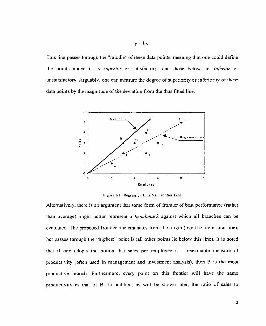
y = bs.

This line passes through the "rniddle" of these data points. meaning that one could define

the points above it as sriperior or satisfactory. and those belobv. as inferior or

unsatisfactory. Arguably. one can measure the degree of superiority or inferiority of these

data points by the magnitude of the deviation from the thus fitted Iine.

O i - 4 b 8 1 O

Em p l o y c e

- -

Figure 1-1 : Regression Line Vs. Frontier Line

Alternatively, there is an argument that sorne form of frontier of best performance (rather

than average) might better represent a b e d m a r k against which al1 branches can be

evaluated. The proposed frontier Iine emanates from the origin (like the regression line),

but passes through the "highest" point B (al1 other points lie below this line). It is noted

thar if one adopts the notion that sales per employee is a reasonable measure of

productivity (often used in management and investment analysis). then B is the rnost

productive branch. Furthermore. every point on this frontier will have the same

productivity as that of B. In addition. as will be shown later, the ratio of sales to

employees. for any branch below the line. is expressible as a measure of the distance of

that point from this line. Thus. the arguably reasonable way of defining performance as a

ratio. can actually be uncovered as a distance from the constructed frontier.

Hence. there esists a fundamental difference between statistical approaches via

regression analysis. and frontier or benchmark approaches. The former reflect "average"

or "central tendenqq" behavior of the observations. while the latter deal with the best

performance. and evaluate the performances of al1 branches as deviations frorn the

frontier line. Thcse two points of view can result in major differences when used as

methods of evaluation. They can also result in different approaches to improvement.

A rrlatively ne\\- efficient?. analysis method. Data Envelopment Analysis (DEA). was

designed to preciselj. construct frontier lines like that displayed in Figure 1-1. Moreover.

it is a tool that is able to do so in a multi output-multi input environment. rendering ir

ideally suited to the problem setting under study. This tool. first developed by Chames.

Cooper. and Rhodes [78CA]. is in widespread use today in a number of areas including

the banking industry. Sherman and Gold [85SG] first used DEA to evaluate 14 branches

of a US salting bank. DEA is a powerful tool that was developed specifically for

determining relative efficiencies within a group of similar Decision Making Units

(DMUs). where a set of outputs. e . g . core deposits. earnings assets, etc.. is created

utilizing severai inputs such as salary expense. numbers of customers. and so on. DEA

calculates a maximal performance measure for each DMU relative to al1 other DMUs in

the observed population. with the sole requirement that each DMU lie on or below the

extrema1 frontier. 1t is a relative benchrnarking tool. meaning that the set of best

practices is based on the particular set of DMUs under study. Typically. this approach is

applied to situations where some factors (both inputs and outputs) are qualitative in

nature. and where conventional engineering approaches to measuring efficiency are of

limired utility. Such is the case in many non-profit institutions. and in the public sector.

With reference again to the simple illustration. DEA would identie a point such as B for

future esamination or to sewe as a "benchmark" to use in seeking improvements. The

statistical approach. on the other hand. averages B along with the other observations.

including F. as a basis for suggesting where improi-ements might be sought.

Although many studies and applications have demonstrated the effectiveness of DEA, it

remains tliat for large-scals problems. with many different factors or variables available,

at least nc.o impedinlsnts to effective implementation still esist.

Fiisr. it is recognized that a DEA analysis entails esplicitly specifying a set of factors to

be used in the modeI. As well. a set of inputs and a set of outputs must be specified for

the analysis to be performed. In many settings. bon-ever. it c m be problematic to define

the most appropriate of those factors to be integrated into the analysis. As with

conventional statistical analysis. many choices c m exist. Equally pertinent. it can be a

challenge to specify which of the chosen factors should serve as inputs. and which as

outputs. Indeed. dependincg on the way the factors are organized. Le.. inputs vs. outputs, a

DEA analysis may result in a particular DMU being classified as inefficient. when, with a

different choice of factors. it may be declared efficient.

A secor~d major element involves implementation. and has to do with management's own

perceptions as to what constitutes good versus poor performance. If a methodology fails

to uncover what management feels is best or worst practice, that methodology is unlikely

to succeed as the measurement tool of choice.

This thesis presents an improved rneasurement tool for evaluating performance of

branches within a major Canadian bank. M i l e there have been nurnerous previous

srudies of performance at the branch level. within the banking industry. this study is

different in a very significant way: specifically two kinds of data are used to develop the

model.

The first type of data is standard transaction data available from any bank. Such data have

formed the b a i s of previous studies. The second type of data. obtained from the site

studied. is n-hat can be called ciass~~cution information. based on branch

consultant'espert judgment as to good or poor performance of branches.

Evaluation of brandi performance by intemal consultants is a common practice in most

major banks. Typically. micro-level work-studies are conducted within a sarnpie of

branches to establish some forrn of standards. While the evaluation of branch

performance attempts to view al1 operational activities as important components of both

the sales and service profiles of the organization, the prevailing emphasis appears to be

on the sales of financial services products (RSPs, mutual funds, etc.). There is usually no

transparent definition of the mechanisms whereby the performance status of the branch is

derived. This is generally due to the attempt of the consultants to merge any computed

quantitative evaluation with factors that capture the environment or context within which

the branch is compelled to conduct its business. This contest c m include the

demographic makeup of the custorner base. such as the financial profile of the average

customer. age. ethnic makeup. and so on.

In most banks. there is seldorn a single and definitive quantitative measure available as to

the performance status of branches. Rather. the practice appears to be to "classify"

branches into two or more groups on the basis of perceived levels of productivity. The

simplest of these classification schemes is a high/low. or good/poor grouping. This is the

case in the present context. and forms the basis of the development in this thesis.

Specificall-. branch consultants have been asked to classify a sample of branches into

two major groups (good performers and poor performers). Arguably. incorporation of

such information into a performance measurement model c m senfe to provide a more

accurate rspresentation of branch et'ticiency. -4s well. any model that builds on such

information is more likely to succeed in being accepted internally.

This thesis demonstrates ho^ this second type of information c m be used in selecting

variables for a DEA analysis in an appropriate way. and can. as well. be used to sharpen

the accuracy of the multipliers applied to these variables in a DEA model.

A major contribution of this work is. therefore. the linkage that it forges between

performance measurement tools (various forms of the DEA model), and the coliection of

tools for classification. e-g. goal programminp. logistic regression and multiple

discriminant analysis. This work is seen as an important and timely step in transforming

the esisting static DEA methodology to a more dynamic performance measurement tool,

along the lines of an expert system. In summary. the thesis develops a DEA methodology

termed EDEA (Expert Data Envelopment Analysis). that combines conventional

6

performance measurement constructs with expert knowledge tools. Such a dynamic

structure will facilitate model updates. and enhance performance measurement accuracy

over tirne.

To provide a backdrop for the model development in the chapters to follow. we briefly

discuss knowledge acquisition. and the basic ideas surrounding expert systems and

artificial intelligence. This provides suppon for. and hopefully validates the contention

that classification information of the type used here is now a valid data source for

performance measurement that deserves attention.

1.2 KNOWLEDGE ACQUISITION

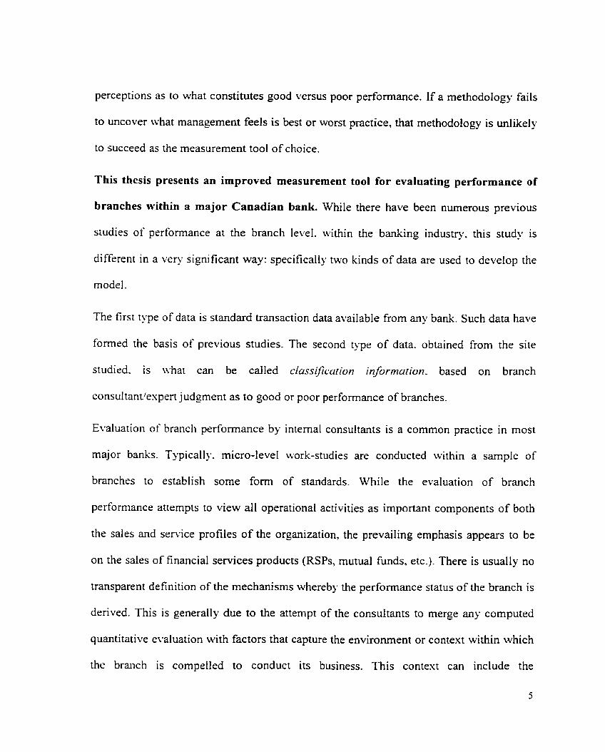
Many areas of research have been developing techniques or approaches to tackle

information that cannot be handled directl!.. because of its "non-sra~zdcr)-d' nature. This is

the case of problems with qualitative data or more sophisticated infom~ation such as

expertise [86B SI.

Figure 1-2: Standard Data Vs. Heuristics

Knowledge acquisition has developed into a mature field. as evidenced by the creation of

artificial intelligence. and more specifically. expert systems. Essentially. the idea of such

systems is to capture the expert's knowledge. and to train the tool to replicate the results

in F~ture.

The expert has a knowledge that the novice does not possess. He also has a recorded and

weli-hown past. proving that he is able to use this knowledge. We rely on experts for

information. their ability to solve problems, and the explmations they give. The

following features characterize them :

Their linowledge is real : the espert can use his knowledge to solve problems with an

acceptable percentage of success.

Their knowled~e is efficient : It is not sufficient to only be able to solve the problems.

an espert can solve them quickll- and efficiently.

Experts know their linlits : An expert is aware of the Iimits to his knowledge. He

knows what hs has to dral with. and when he must rely on others.

Kno~vledgs acquisition techniques use methods in order to gather and organize experts'

knowledge in a form that can be adapted to hardware and to analytic models. These

methods are based on a range of ideas sternming fiom several areas.

The classification techniques involve presenting to the expert the objects to be classified.

Thus. Lve obtain a hierarch which can either be simple (rwo groups). or complex.

according to the cases involved (several groups or hierarchical networks). Thus, one can

see that such techniques can be used to better formalize complex information. Their

ad~~antages are to gi1.e more data. and improve objectivity. thus leading to better models

or systems.

The knowledge acquisition principles can be applied in fields such as DEA. Indeed, we

often have quantitative data available conceming agencies' activities. but seldom use

qualitative information. such as environmental data or the expertise of branch

consultants. The objective herein is to design a construct to capture as much information

as possible. by taking into account this espertise. and thereby produce improved DEA

models. Knowledge acquisition is an iterative and continuous process. This process can

be divided into four major steps:

Acquisition: The bank branch consuItants have provided standard data such as the

number of employees and the nurnber of RRSP sold per branch (Table 111-1). In

addition. as pan of their expertise. they have dassified a set of branches into two

groups: specifically. lotv and high perforrning branches:

Formulation: We use the standard data to build the DEA models. and then utilize

discriminant techniques and operational research 1001s to formulate and integrate the

branch consultant expertise into these models:

Transfer: The entire set of information provided by branch consultants (standard data

and espertise) is integrated into the selected DEA models. to compare their

performance rvith "classical" DEA models. and thus demonstrate the possible

improvements that can resuh:

Test & Validation: The models thus obtained are tested and used to provide

benchrnarking resulrs that can aid branch consultants in managing the branch

network.

Figure 1-3: Knowledge Acquisit ion T o Irnprove DEA hlodels

In the chapter to follow. we review some of the basic DEA and classification models.

This \vil1 pro~pide the necessary fiarnework for the development in Chapters 3-5.

Conclusions are presented in Chapter 6.

II. OVERVIEW OF PERFORMANCE MEASUREMENT MODELS AND CLASSIFICATION TOOLS

11.1 DATA ENVELOPMENT ANALYSIS MODELS

11.1 .l The concept

Data Envelopment Analysis (DEA). a frontier analysis tool, is a special application of

linear programming based on Farrell's frontier methodology [57FM] as advanced by

Chames. Cooper and Rhodes [78CA]. and Banker. Chames, and Cooper [WBR].

DEA compares the inputs and outputs of Decision-Making Units (DMUs) and assesses

their relati\.e efticiency. .A DMU is a basic entity (e.g.. a bank branch) utilizing several

inputs to produce a set of outputs (Figure 11-1 ). that the decision-maker wishes to analyze

and rank nithin a comparable set of entiries (DMUs). DEA calculates a masimal

performance measure for sach DMU r-elariiv ro al1 other DMUs in the observed

population. with the sole requirsment that each DMU lie on or below the estremal

frontier. It is a relative bencharking tool. which means that the set of best practices is

based on the set of DMUs being considered at the time. Each time a new DMU is

included in the samplr. the set of best practices and the efficient frontier have to be

recomputed.

gure II-! : ri Bank Branch

The DMUs found to be inefficient are stnctly inefficient in a Pareto sense in that at least

one other DMU can produce at least the sarne outputs using less inputs. A significant

feature of DEA is that it allows for the inclusion of multiple input and output variables

that are calcuiated simultaneously. This ability sets DEA apart from the other single

dimension analytical techniques generally used in comparative analysis (e. g.. ratio

analysis and regression analysis). It is. thersfore. a performance measurement technique.

\vhich can be used for evaluating the relative efficisncy of DMUs in organizations.

Conventional ratio analyses give different pictures depending on the particular analpzed

ratio. In addition. it is difficult to combine an entire set of ratios into a single judgement.

This n.ould be especiall). true i f one wcre to increase the number of Dh,ILs.

In contrast to pararnetric approaches ~vhose objecti\.e is to optimize a single regression

plane through the data. DEA optimizes on each indi\.idual observation with an objective

of calculating a discrete piecet\-ise frontier. the efficient frontier. dettirminsd b). the set of

Pareto-efficient DMUs (Figure 11-2).

Pîrarnetric approaches require a specific functional forni (e.g.. a regression equation. a

production function. etc.). relating the independent \.ariables to the dependent variable(s).

The functional form selected also requires specific assumptions about the distribution of

the error t e m s (e-g., independently and identically normally distributed). and many other

restrictions. In contrast. DEA does not require any assumption about the functional form.

O O 5 10 15 20

INPUT -- - - --

Figure 11-2 : Cornparison Of DEA And Regression Analysis

The purpose of DEA is to find the best strategy to bring inefficient DMUs (belou. the

efficient frontier) ont0 the efficient frontier. either by reducing their inputs (the use of

their resources such as the number of cashiers), or by increasing their outputs (irnproving

somr parameters such as the numbers of operations per hour). This is illustrated by

Figure II-;.

By projectin each unit ont0 the frontier, it is possible to determine its Ievel of

inefficiency bjr comparison to a single reference unit or to a combination of reference

unirs. The projection refers to a vinual efficient DMU, which is a combination of one or

more efficient DM&. Thus. the projected point may itself not be an actual DMU.

I For the additive rnodel we can cornpute the corresponding efficient DMU of every DMUj by using the following projection: .y, . )-, 1 + ( .\' , . f , ) = (.y, - s-', 1; + ) . The slacks for an efficient DMU are both

nul!. Thus. this formula wiil give the DMU itself if it is an efficient one (identity mapping for efficient DMUs). See the surnrnac. tables for the projections of each rnodel.

INPUT

. .

Figure 11-3 : Enveloprnent Surface For The Additive hlodel

In summary. the DEA approach offers three main features:

1. Characterization of each DMU b!. a single summary relative-sfficiency score;

2. DMU-specific projections for irnpr~\~ements bascd on best-practice DMUs; and

3. Obviation of the alternative and indirect approach of specieing abstract statistical

models. and making inferences based on residual and parameter coefficient analysis.

11.1.2 DEA Models

DEA. in e\-aluating an!. number of DMUs. with any number of inputs and outputs:

Requires the inputs and outputs for each DMU to be specified:

Defines efficiency for each DMU by an objective function. The objective function in

DEA can be ratio oriented (outputs!inputs). or net protit oriented (outputs - inputs);

In calculating the efficiency of a particular DMU. weights are chosen to maximize its

efficiency. thereby presenting the DMU in the best possible light.

L 1 I 1 Figure I I 4 : DEA Ratio And Net Proiit Oriented Models

Man', DEA models and extensions can be found in literature. The main ones are the

additive model and the extended additive mode1 [87CA]. the multiplicative models

[83C.A]. the CCR (Charnes. Cooper and Rhodes) mode1 [78CA]. the BCC (Banker.

Charnes. and Cooper) mode1 [84BR]. and their ratio counterparts. Each model can have

different options. We discuss only the CCR. BCC. and additive models herein.

Ratio oriented models

11.7.2.1 DEA Mode1 Options

DEA offers three different orientations; input-oriented models, output-oriented models

and additive oriented rnodels (also called base-oriented models). Each of these

orientations can ha\.e constant returns to scale or variable returns to scale.

Net profit oriented models

In the input-oriented models, the inefficient DMUs are projected ont0 the efficient

frontier bl. decreasing their consumption of inputs. Input minimization allows us to

determine the estent to which a DMU can reduce inputs while maintaininç the curent

le\.el of outputs. This might occur in a situation where competition limits the market for

finished goods.

In the output-oriented models, the inefficient DMUs are projected ont0 the efficient

frontier by increasing their production of outputs. Output rnaximization might be used

when the inputs are constrained, such as by a fixed allocated budget, and the emphasis is

on increasing the outputs.

In the base. or additive models. inefficient DMUs are projected ont0 the efficient frontier

by simultaneously reducing their inputs and increasing their outputs to reach an optimum

level.

Figure 11-5 is an illustration of these possible orientations. The efficient DMU P5-1 is the

input projection of the inefficient DMU P5. Similarly. the efficient DMU P5-0 is its

output projection. and P2 is its base projection. However. there are cases where an input

reduction or an output increase u-il1 not be sufficient to make a DMU efficient because of

the fronrier boundaries. In such cases. additionai movement toward the envelopment

surface ma!. be necessar!. via an input reduction (DMU P7) or an output augmentation

(DMU P6).

O 2 4 6 8 10 12

l NPUT

Figure 11-5 : DEA hlodel Orientation

The constant retums to scale (CRS) model assumes that one unit of input results in a

constant nurnber of units of output (Figure 11-6). The variable returns to scale (VRS)

model assumes that one unit of input can result in a number of units of output. where this

number can be different at any point on the input scale. In the VRS model. DEA

determines the relationship (positive or negative) as well as the size of the retums to

scale. This provides flexibility to test different scenarios of performance based on

different assumptions. Additionally. under the VRS rnodel, one can explore the impact of

input minimization or output maximization.

O 2 4 6 8 1 O 12

INPUT

Figure 11-6 : Envelopment Surface For The Additive Mode1

The computing process is the sarne for any model. Given a set of n DMUs. the model

deiermines for each DMUo the optimal set of input weights and output weights that

optirnize its efficiency score under the set of constraints represented by DMUs in the

cornparison set. The objective funîtion gives the efficiency score o f the DMUo. This

process is repeated n times- once for each DMU, that has to be rated.

11.1.2.2 Efficiency measures in DEA

As can be seen in Figure 11-6, an efficient score can be computed for every DMU. This

efficient score is based on the efficient frontier and the projection o f the DMUs to this

frontier. Thus, the efficiency depends on the model itself. For a given DMU,. the input-

D, oriented efficiency score. for example, is given by the fol lo~ing formula: E, = - .

D,

where Dj is the distance of the DMUj from its projected point on the output axes and 8,

the distance of its projecred position on the fiontier fiom its own projection on the output

axes. For instance. the efficiency for the DMU, in the case of the VRS model is

AP. E- =- while the efficiency for the DMUl is E, = - AP3 = 1 = 100% . A P- A 4

This figure also illustrates the impact of a CRS model on the efficient fiontier and the

efficiency scores. Indeed. this model relaxes the convexity constraints. which reduces the

number of efficient DMCis (P I . P; and P7 are nu longer efficient). and ofien lowers the

efficiency scores of the inefficient DMUs. With this model. the same DMU7 has a score

clearly smaller than with the VRS model:

The following sections present the principal DEA models with their characteristics and

properties. We highlight specifically the basic radial projection models. and the additive

or base model. We do not discuss. herein, models such as the multiplicative DEA

structure. These models are the application of the additive models to the logarithrns of the

original data values. Therefore. the interpretations of the additive models apply, but in the

transformed logarithmic space. They yield log-linear envelopment surfaces.

1 . 2 3 The CCR Model

The CCR [78CA] model determines the set of weights that maximizes any DMU

efficiency relative to other DMUs of the sample. provided that no other DMU or convex

combination of DMUs could achieve the same output vector with a srnalier input vector.

In the input-oriented model (Figure 11-7): the objective is to produce the observed outputs

using a minimum level of resources.

Figure 11-7 : Envelopment Surface For The CCR-1 Mode1 (CRS)

In the output-oriented mode1 (Figure 11-8). the objective is to produce the maximum ievel

of outputs gi\*en an observed level of inputs.

O 2 4 6 8 10 7 2

INPUT

Figure 11-8 : Envelopment Surface For The CCR-O Model (CRS)

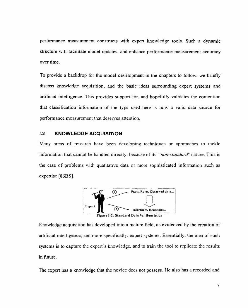
11.1.2.3.1 The CCR Ratio Formulafions

The CCR ratio formulation was the first standard DEA mode1 proposed by Charnes,

Cooper. and Rhodes [78CA]. The ratio formulation allows one to consider multiple-input.

multiple-output situations. Indeed, the mode1 reduces these situations to that of a single

"virtual" input and a single "virtual" output. As we c m see. for the CCR Ratio

formulation. a change in the orientation simply amounts to inverting the ratio. For

instance. the CCR-IR masimizes the production of the outputs while minimizing the

utilization of the inputs.

The CCR Ratio Formulations CCR Input Ratio (CCR-IR) CCR Output Ratio (CCR-OR)

These ratio formulations are very useful from an engineering point of view. However.

the). >.ield an infinits number of optimal solutions [93CA].

/1.1.2.3.2 The CCR Linear Formulations

Chames and Cooper [62CA] developed a transformation of these ratio formulations using

linear fractional programming and a representative solution (vTxo=l). Consequently. by

replacing the expression vTxo with 1. each of these formulations can be solved using their

corresponding net profit oriented mode1 formulations. Figure 11-9 sumrnarizes the mode1

equivalencies. The follo\ving figure presents the prima1 and dual input formulations of

the CCR linear model. There are CCR output oriented linear rnodels as weI1, but we will

not present these here. A DMU is efficient in a CCR input oriented model if and only if it

is efficient in the corresponding CCR output oriented model.

A small non-archimedian infinitesimai E has been introduced to prevent the zero weight solution [83CA].

The projectrd coordinates for an' DMU are: + ex, - S- ; y. + Y, + St

The CCR Linear Formuiations

The absence of the convesity constraint reduces the number of efficient DMUs and

results in a constant returns to scale envelopment surface (Figure 11-6).

Input-Oriented CCR Prima1 (CCRp-1) - - Adin z,, = B -E. 1s- - E . 15-

d ;..\- . \

S.[ .

1-2 - s- = 1;

&Y,, --Y2 - 5 - = O

%.s* .s - 2 O

We might have some cases where the proportional input reduction by itself may not be

sufficient to achieve efficiency; specifically, we might have to reduce some inputs and

augment some outputs (positive input and output slacks are frequently necessary to reach

the envelopment surface). This is common with multiple inputs and outputs problems.

Input-Oriented CCR Dual (CCRD-1)

Max wo = ,ury0 p.r

SJ*

vrx, = 1

~ ' Y - V ~ X 5 O -

pT 2&.1 -

v r 2 E. 1

11.7.2.4 The BCC Mode1

11.1.2.4.7 The BCC Ratio Fomulations

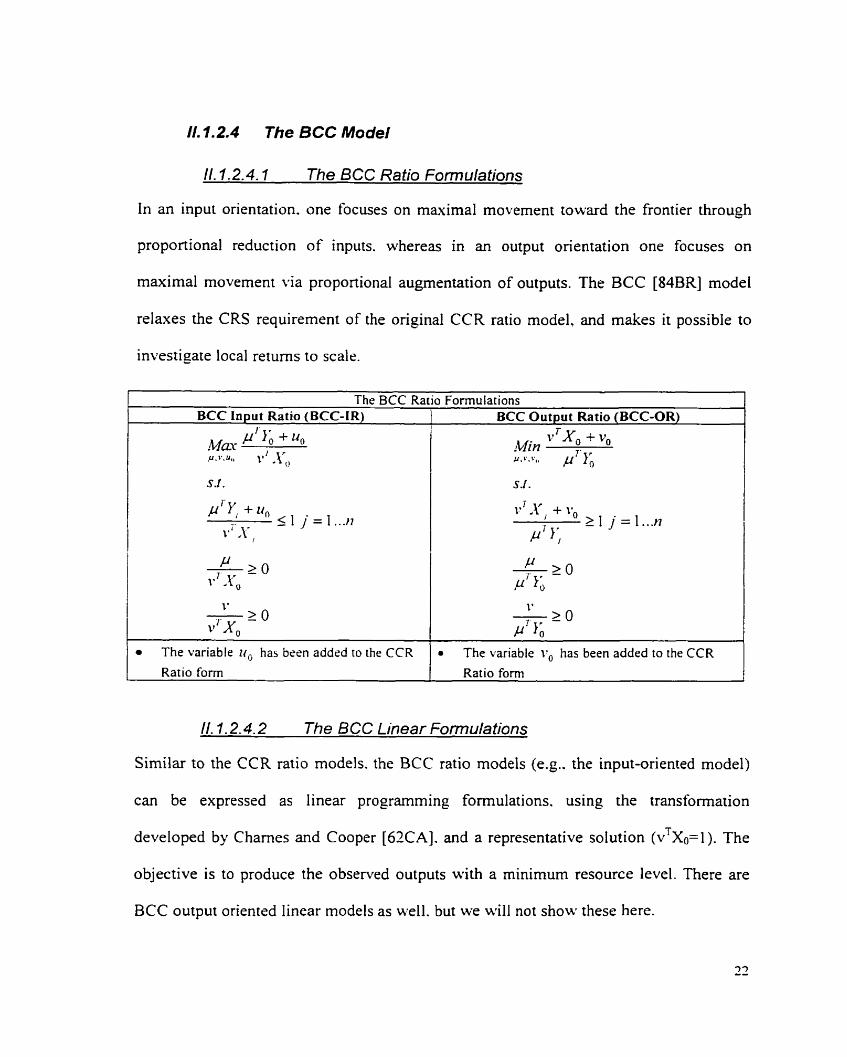
In an input orientation. one focuses on maximal movement toward the frontier through

proportional reduction of inputs. whereas in an output orientation one focuses on

maximal movement via proportional augmentation of outputs. The BCC [84BR] mode1

relaxes the CRS requirement of the original CCR ratio model. and makes it possible to

investigate local retums to scale.

S.I. I

The BCC Ratio Formulations

- - - --

The variable I r , has been added ro the CCR-IT The variable iTo has been added to the CCR

BCC Input Ratio (BCC-IR)

+ u, M a . P.'..., ,*l'.\r()

BCC Output Ratio (BCC-OR)

v T x , + v, min P.'.',, p7'&

II. 1.2.4.2 The BCC Linear Formulations

Ratio forrn

Similar to the CCR ratio models. the BCC ratio models (e.g.. the input-oriented model)

can be expressed as linear programming formulations. using the transformation

developed by Chames and Cooper [62CA]. and a representative solution (vTxo=l). The

objective is to produce the observed outputs with a minimum resource level. There are

BCC output oriented linear models as well. but we will not show these here.

Ratio forrn

I f a DMU is efficient in a CCR model it will also be efficient with the BCC modeI. but

the converse does not nocessarily hold [88BR].

The BCC Linea Input-Oriented BCC Primal (BCCp-1) - -

Mit? Z, = 8 - E. Is' - E. Is- t I . i . \ * . b

r Formulations Input-Oriented BCC Dual (BCCD-1)

7 M a y rr, = p Y. + tc, p.)'

Sf.

i " ~ , = I

1 The scalar variable 0 is the proportional reduction applied to al1 inputs of DMU,. A DkIU is efficient if and on[>. if û* = 1 and al1 slacks are zero.

Or. a DMU is efficient if and only if Z; = il{ = 1 . An!. non zero slacks and the value 0* <= I identiQ the sources and amount of inefficiencies that may be present. The projected coordinates for an' DMC on the efficient frontier are:

,Y, -P &Y, -s- : 1; + 1; -t s-

Figure 11-9 is an illustration of the relations between ratio and linear DE4 formulations.

For esample a CCR input ratio model can be transforrned into a CCR input linear model

by using the solution \?io = 1.

vTX,= I CCR-IR < CCRp-1

CCR-OR CCRD-O

I.~S, ,= I CCR-OR < > CCRp-O

Figure 11-9 : Ratio Vs L

vT.L ,= 1 BCC-IR BCCD-I

vTX ,= 1 BCC-IR BCCP-1

BCC-OR BK,-O

vTX, = 1 BCC-OR Bcc~-O

near DEA Formulations

i . 2 5 The Additive Model

As illustrated in Figure 11-5. the additive (or base) model projects along both output and

input dimensions. The additive model selects the point on the envelopment surface that

maximizes the L I distance in the "nonhwesterly" direction (reduces the inputs and

increases the outputs). This model has variable retums to scale and the efficient frontier is

invariant with respect to an affine translation of the data (consequences o f the convexity

constraint in the prima1 problrm or the unconstrained variable uo in the dual).

The Additive Model Additive Prima1 (ADDp) l- Also calfed the Envelopment Form - - M i 1 7 = - 1 s * . - - - 1 s -

K . % . \

- - 2.5 .s 2 0 n : number o f DMUs Y : marris o f output measures X : matris o f input measures

Additive Dual (ADDD) Also called the Multiplier Form

7 Alm Il-(, =,Y Y. - leJ -Yo + uo , U . 1 ' . l i , ,

s* and s- : siack variables on inputs and outputs

DMUo is efficient if and onl? if Z: = i1.I = O

DMUo is inefficient if and only if s*' # O or s-' # O The projected coordinates for an' DMU on the efficient fronrier are:

11.1.3 Major DEA Model Extensions

In realistic situations. one might need to incorporate some variations into the DEA

2 4

models such as non-discretionary variables. categorical inputs and outputs. and

qualitative data factors. We might also want to incorporate judgment or a priori

knowledge in the form of restrictions on variable rnultipliers. Because non-discretionary

variables are beyond control of the DMU's management. they will be excluded from the

objective function of the model but not from the constraints. With categoncal inputs and

outputs. one could run different DEA models for each category by following a

hierarchical process based on the hierarchy of the categories. Judgment or a priori

knowledge allows the analyst to tune hislher model in accordance with hisher knowledpe

of the situation. One will be able to restrict the range of the multipliers. for example.

11.1.4 Strengths and Limitations of DEA

DEA provides a new approach to organizing and analyzing data ("discussing ncu- truth").

It demonstrates that by the use of another methodology. unanticipated insights ma' be

obtained and ma'. therefore. redirect managerial action. The DE.4 framework creates a

new approach for learning from outliers and for applying new theories of best practice. It

provides a mors comprehensive picture of organizational performance. In fact. DEA

seems to be a very suitable tool that offers the possibility of handling multiple inputs and

outputs stated in different measurement units. It focuses on a best practice frontier instead

of the population central-tendencies: the inefficient DMUs are compared to their

projected efficient DMUs in order to analyze their inefficiencies. The multiple DEA

variations allow one to address many managerial problems by taking into account their

own properties (limited inputs and/or outputs, for instance).

DEA. as with other concepts has some limitations not yet resolved and some unexplored

dimensions. Noise in the data. even symmetncal noise with zero rneans. such as

measurement error. can cause significant problems. Statistical hypothesis tests are

difficult and are the focus of ongoing research. Finally. the standard formulation of DEAS

which creates a separate linear program for each DMU. c m be computationally intensive

for large problems.

In this section the basic DEA models have been exarnined. In the section to follow. some

of the standard models for handling classification data are discussed. It is emphasized

again. that the mode1 structures devsioped in later chapters are designed to evaluate those

situations where standard numerical data in a DEA setting is augmented with

classification data. Hence. there is a need to examine which classification methodologies

best suit this linkage essrcise.

11.2 DISCRIMINANT MODELS

In this section we review some of the standard classification rnodels. Specifically. we

examine logistic regression. multiple discriminant analysis. and goal prograrnrning.

11.2.1 Logistic Regression

/1.2..1 Introduction

The logistic regression technique [94DK] analyzes the relationship between dependent

(or response) variables and independent (or explanatory) variables. The dependent

variables are always categorical. while the independent variables can be categorical

(factors) or continuous.

When we study a random ~eariable Y using a linear model. we specify its espectation as a

h'

linear combination of K unknown parameters and covariates.: E ( Y ) = ,u = P, x, . k

We introduce a more generalized forrn called the link function: >I = g ( p ) .

The link function defines the mode1 used. which c m be determined by the distribution of

the randorn component. The distribution of the random component in Y (the part that

cannot be systernatically esplained by s variables) determines the type of generalized

linear rnodel (Figure 11-1 O). The distribution of the randorn component cornes from an

exponential family. to which the normal. binomial. and Poisson distributions beIong.

Ordinary Least Squares (OLS) assumes the normality of this distribution. while the Logit

and Probit models are both based on the binomial distribution.

Logistic regression has the advantage of being less affected than multiple discriminant

analysis (MDA) when the basic assumptions, particularly normality of the variables, are

not met. It also can accommodate non-metric variables through dummy-variable coding,

jus1 as regression c m . It is limited, however, to prediction of only a two-group dependent

measure. Thus. in cases where three or more groups form the dependent measure. MDA

is best suited.

Distribution of the Lin k Function

Binomial Logit

--

Binomial Probit = ' P h is

the inverse of the standard normal cumulative distribution function

Poisson Logarithm 7 = log(^)

Multinomial Multinomial Logit P q = l o g ( L ) j = 1, ..., J

PJ Figure 11-10: hlodet Classification Based On The Distribution OfThe Random Cornponent

Logit models have only two categories in the response variable - event A or non-A. The

response variable y is a realization of a binomial process.

We may express logit models in probability form:

The probability of non-event is then:

By simplifying. we O btain:

Therefore. we can state that:

The fraction - is called the odds ratio. Norv. take the natural log of the odds ratio: 0 - p, )

J11111 lim Prob(1' = 1) = l und lim Prob(I' = l ) = O ,$;-++x p. r - -cc

L ' is called the logit. and hence the name logit model' (Figure 11-1 1) .

I L, the log of the odds ratio, is not only linear in X. but also (fiom the estimation viewpoint) linear in the parameters. However. Although L is linear in X. the probabilities themselves are not. This property is in contrast uith the LPM model where the probabiiities increase linearly with X. ' The interpretation of the iogit model is as follows: the P, measure the change in L for a unit change in x,. The intercept P, is the value of the log-odds when X =O. Like most interpretations of intercepts, this interpretation may not have any physical meariing. Given a certain x,, if we actually want to estirnate not the odds in favor of being solvent but the probability of being solvent itself, this can be done directly fiom

I once the estimates of p l and p, are available. J + exp(-(P, + P, -Y, 1)

-- - O

Figure 11-1 I : Logit Üesponse ~ u n c t i o n

2 1.3 The Maximum Likelihood Estimation

Estimation of binary choice rnodels is usually based on the method of Maximum

Likelihood. Each observation is treated as a single draw frorn a Bernoulli distribution

(binomial with one draw - Figure 11-1 0). The mode1 with success probability F(P's)' and

independent observations leads to the joint probabili ty. or Iikelihood function:

By stating that P, = F(Ptx) , this formula can be rew~itten more conveniently as

Since it is easier to work with sums than with products we start by taking logarithms.

h(L) = x[i; L ~ P , + ( 1 - Y, )Ln(l - P, )] I

Maximizing the likelihood L is equivalent to mavimizing the Log Likelihood Ln(L).

Therefore. the first derivatives are computed with respect to each of the K coefficients PL,

and set to zero. The solutions of these K equations. called the likelihood equations. will

give the Maximum Likelihood &timation2 (MLE) estimators. The logit iikelihood

equation c m be written as:

Where the term in brackets is the deviation between the observation Y i and its expected

\-alue. X , are the weights.

1 The general Framework of probability models is: Prob(Y = 1 ) = F(P'x) and Pmb(Y = 0) = 1 - F(P'x). ' The minimum chi-square estimation for replicated. dichotomous data is an alternative to maximum likelihood estimation.

11.2.2 Multiple Discriminant Analysis

11.2.2.1 Introduction

The basic purpose of multiple discriminant analysis (MDA) is to estimate the relationship

between a single nonmetric (categorical) dependent variable (groups) and a set of metric

independent variables (predictors). The MDA can classify more than two groups'. When

two classifications are involved. the technique is referred to as two-group discriminant

analysis (DA) in contrast kvith MDA.

The MDA identifies the areas m-here the greatest difference exists between the groups.

derives a discriminant weighting coefficient for each variable to reflect these differences.

and then assigns each indi\.idual to a group using the weights and each individual's

ratings on the characteristics. The ultimate goal in MDA is to predict to which group a

new observation belongs.

11.2.2.2 Discriminant Analysis Model

MDA is based on centroids2 and groups (Figure 11-12). The centroids indicate where the

groups are centered or located. In general. the more centroids for the groups differ. the

easier it is to distinguish between the groups. However, most of time the difficulty is to

distinguish the groups when there is an overlapping area.

[ Problems involving only two groups could be handled with lest squares regession. ' A centroid is the mean value for the discriminant Z scores for a particular category or group. A two-group discriminant analysis has two centroids. one for each of the groups.

.\ Figure 11-12 : Discriminant Analysis Centroids

MDA involves deriving the linear combination of the two (or more) independent

variables that \vil1 discriminate best between the a priori defined group. This is achieved

by the statistical decision rule of maximizing the between-group variance relative to the

within-group variance. This relationship is expressed as the ratio of between-group to

within-group variance (Figure 11-13). It is similar to maximizing the between-group

variance and minimizing the within-group variance. If the variance between groups is

large relative to the variance within the groups, we say that the discriminant function

separates the groups tnell (Figure 11-1 4).

MDA Ruie

MAX ( Between - grorrp var iance) Benveet~ - group variance Ifirhir~ - group var lance ] 0 ami

MIN(WÏrhitr - groirp var tance)

Figure 11-13 : M D A Ruie

The linear combinations for a discriminant analysis are derived from an equation that

takes the following fom:

1

2, = Discriminant score

= Discriminant weight for the jIh observation and the i l h variable

X, = id' Independent variable for the jth observation I

The centroids for the two groups. Cl and C2. are the average discriminant scores of al1

the observations within each group. They indicate the most typical location of an

observation from a particular group' and a cornparison of the group centroids shows how

far apart the groups are along the dimension being tested.

The test for the staristical significance of the discriminant function is a generalized

measure of the distance betkveen the group centroids. This is done by comparing the

distribution of the discriminant scores for the two groups. If the overlap in

distribution is small. the discriminant function separates the groups well.

the

-- Figure 11-14 : M D A Overlapping Distributions

11.2.2.3 Determining the Cutoff Value

There are different ways to determine an appropriate cutoff value. One way would be to

select the cutoff value that minimizes the number of misclassifications in the analysis

sample. Another way would be to select the cutoff value as the midpoint between the

centroids of the groups:

Here Ni and N2 are. respectiveIl.. the numbers of observations in groups 1 and 2. Figure

11-15 is an illustration of the cutoff \ralue ~vhen the two group sizes are equal and

differenr. The right-hand side shows tw-O cutoff values: the unweighted cutting score does

not take into account the Sroup sizes. and thus leads to a poor classification.

Optirnrl iut:ins 5 id rc iiith cqual urriplc ,ire\

Figure 11-15 : %IDA Optimum Thresholds

Generally. MDA attempts to minimize the oïerlapping area b e t w r n groups. Depending

on how data are distributed. these cutoff value approaches can lead to poor classification

results. Therefore. we use a more refined cutoff value. which considers the cost of

misclassifying an obsenration into the wonp group. The optimum cutting score will be

the one that minimizes the cost of misciassification. It is represented by:

LN(.): natural logarithrn

, (q - l)$, + (17: - l)s;, SE, =

n, + nI - 2

C( 1 12): the cost of classifiing an observation into group 1 when it belongs to group 2.

C(2ll): the cost of classi-ing an observation into group 2 when it belongs to group 1.

P l : the prior probability that a new observation belongs to group 1 .

P:: the prior probability that a new observation belongs to group 2.

.4 more re fined formula is sometimes used. the Mahalanobis distance measure. which

takes into account the differences in the covariances between the independent variables

[97GR'].

11.2.3 Linear Goal Programrning Discriminant Models

II. 2.3.1 Introduction

Linear goal programming (GP) is a polverful extension of linear programming (LP). The

goal prograrnming approach is probablj. most popular for handling multi-objective

problems. It has the added conveniences that different objective fùnctions can be

measured in different units. and that it is not necessary to have al1 the objective functions

in the same forrn (masimization or minimization).

The first step in fomulating a GP mode1 is to create a constraint for each goal in the

problem (Figure 11-16). This allows us to determine hou- close a given solution cornes to

achieving the goal. Thus. a goal can be viewed as a constraint with a flesible Right-Hand

Side (RHS) value.

The RHS value of each constraint is the target value for the goal because it represents the

level of achievement that the decision-maker wants to obtain. The ~rariables d,+ and d,- are

called deviational variables. in that the' represent the amounts by uhich each goal

deviates from its target \value. The d,* represents the amount b!. ivhich each goal's target

value is underachieved. and d,- the amount by which each goal's target value is

overachieved ' .

1 1) In goal programming it does not make any sense for both deviational variables to take non-zero values simultaneously. In fact. due to the nature of the solution process. we do not have to model this condition. 2 ) In a GP problem. not al1 constraints have to be goal constraints. .4 GP rnodel can also include one or more hard constraints typically found in LP problems.

l I

Goal constraint formulation

1 1 Dscision variables 1 1 RHS = Target Value 1

1 Deviaiional variables I 1

Figure 11-16 : Goal Programming Constraint

The objective in a GP problem is to detemiine a solution that achieves a11 goals as closely

as possible. The ideal solution to any GP problem is one in which each goal is achieved

esactly at the level specified by its target value (d,- = d,- = O). One possible objective

(many variations are possible and depend on the probIem itself) would be to minimize the

sum of the deviations:

Min x ( d , + tri:)

Based on these principles. mode1 formulations depend on the problems treated and the

decision-maker's objectives. Indeed, some goal constraints will be more important than

some othrrs. or the objective function ma? emphasize one specific goal being reached

before some others would (preernptive goal programming). We can find many variations

in the literature [90GF]. One of them is the use of goal programming as a dis cri min an^

11.2.3.2 Goal Programming Discriminant Models

Applications of linear goal prograrnming-based approaches in discriminating between

two groups of observations. have appeared in numerous publications [95GF]. The main

idea here is that with GP models. we seek a hyperplane to separate two groups of points

"in the best possible way". regardless of whether or not they can be completely separated

[90GF].

A goal programming discriminant problem will have three parts:

1 . The objective function. which determines the way the model will solve the problem.

If the objective is to minirnize the number of misclassifications, we will use models

such as integer programming ($ 11.2.3.2.1). If the objective is to minimize the total

amount of esternal deviations and masirnize the total amount of intemal deviations

from the separating hyperplane. Ive will use models such as Giover's formulations

(9 11.2.3 .X) .

2. The constraints. representing the observations of each group. will be espressed

according to the model and the objective function.

3. The extemal constraints. not rea1Iy based on the model but necessary to reach an

optimum solution and avoid some problems such as the zero solution.

Many difficulties arise m-hen we try to discriminate between overlapping groups. Some

formulations have been proposed to handle these cases [86GF]. They al1 depend on the

problem itself and the objectives sought. The. could be of simple linear form,

incorporating variables such as interna1 and estemal deviations, or of a more complex

form. using quadratic. power or logarithrnic models.

11.2.3.2.1 lnteaer Goal Programmina Mode1

The integer programming formulation. where the objective is to minimize the nurnber of

misclassified points, c m be stated as follows:

subject to :

A , x - M y , <b i E G,

-4, x + iLI7, > b i E G?

7. E ~0.1) I. b wu-estricted in sign

A,. i E GI. represent the points of group 1 and A,. i E G?. represent the points of

group 2 (A, is an n-vector in Euclidran space):

x is the associated n-vector of variables that weight the points A,:

b is the scalar variable (The Threshold):

M is a large positive nurnber and is related to the esternal deviations. which a i s e for

points on the wrong side of the hyperplane (improperl?. classified):

-J, are binary integer variables (O or 1). which are used to count the number of

violations;

The discriminating ability of this mode1 can be improved by adding an infinitesimal

parameter. Say E: which avoids having some observations lying on the hyperplane

(neither in the group 1 nor in the group 2).

subjeci to : A , x - My: < 6 - E ~ E G ,

.-l,s+My, > b t & k G 2

7, E (0.1) .Y. 6 rrnrestricted in sign

In Figure 11-17. we can see how the mode1 discriminates between groups. A circle

represents the observations from group 1 and a star, those from group 2 . As we can see

that observations 2 and 5 are misclassified. Therefore, their corresponding y variables

\si11 take on the value of 1. and the others will be zero. The value of the objective

function will be 2. meaning two misclassified observations are present.

Group Differentiation with Integer Programming

Croup 2

Figure 11-17 : Illustration Of Integer Programming Discriminant Model

11.2.3.2.2 Glover's Fornula fion

Glover. in [90GF] introduces two models based on the same assumptions. but differing in

the way they handle the points lying on the hyperplane. The full model introduces two

variables a0 and Po, whereas the reduced mode1 uses an infinitesimal variable. B. In fact,

the full model can be formulated with or without E, but it is not recomrnended pnmarily

because it induces a redundancy. and makes the interpretation more difficult.

Full mode1 (with or without E) Reduced Model

s, b unrestricted in sign

Minirnize ~ l l n , - ~ k , f l

subject to :

( I ) . . i ,x -a , +P, = h - r ~ E G ,

(2).4,s+ori -Pr = b + r i~ G,

(;)a, 2 O

(3)P. 2 0

( 5 ) n , X ( P 1 -a.)+q Z(P, -a.) = 2n,n2 f * 1;, .cc;.

x. b unrestricted in sign

Where : A,. i E G I - represent the points of group 1 and Al. i E Gz. represent the points of group 2 (A, is an n-vector in Euclidean space); s is the associated n-vector of variables that weight the points .A1: b is the scalar variable; a, represent the external deviations. which arise for points on the \+Tong side of the hyperplane (improperly classified): pi represent the interna! deviations, which &se for points on the correct side of the hyperplane (properly classified); h, and ki are the coefficients that weight the external and internal deviations in the objective function; a,-, represents the maximum externa! deviation; Po represents the minimum internal deviation: ho and ko are the coefficients that weight a0 and Po; nl and nz are, respectively. the numbers of points in groupl and group 2: E is a non negative parameter utilized to induce a strict separation between the groups.

32

The goal is to minimize the weighted surn of extemal deviations and maximize the

weighted surn of intemal deviations (Figure 11-18). In problems where it is especially

imponant to correctly classify certain observations. those observations can be weighted

by increasing the appropriate h, and k, values in the objective function. Applying equal hi

and k, weights to both groups of data implies that the cost of a Type 1 error is equal to the

cost of a Type II error.

An example M-here Type 1 and Type II errors deserve different emphasis c m be the

following. N'hile tqing to identify banks that will succumb to bankruptcy. it ma' be

more important to be assured that a bank classified as financiallu strong will in fact

escape bankruptcy than to bs assured that a bank classified as financiall>- weak will

become insolvent. In addition. with the capacity to give higher weights to banks that are

dramatically successful or unsuccessful, the LP formulation will tend to position the "sure

bets" more deeply inside thsir associated half spaces. It is also a way of isolating these

cases that are difficult to discriminate. or even those that ~rould be considered as outliers

[90GF].

Group Differentiation with Overlapping Groups

I I I --

Figure 11-18 : Goal Programming Classification W'ith Overlapping Groups

The normalization constraint (constraint 5 in full and reduced models) is equivalent to

requiring a meaningful separation, and eliminates the nul1 weighting x=O as a feasible

solution. Glover in [89GF] has shown that the LP formulation employing the

normalization is a direct relaxation of a corresponding integer programrning problem for

minimizing the number of misclassified points.

Note that it is possible to obtain an LP discriminant analysis formulation that does not

require a normalization by relying on an objective function that is either derived from

regression analysis or that represents a norrnalization itseIf.

Even if some formulations tend to discriminate "well enough". it remains that for man-

problems. difficuities in efficient]! segregating groups will occur. due to degeneracy. as

has been pointed out in [86GF] : ". . . I A ~ S L ' CUSES represenr norhing pa[hologicul. Szrch un

ozrrconte nlerel~. signals [hm rhe grozdps cannor be separated, and thar rhe forin of group

oi*erlap co~fozrrids an). rensonuble 'purrial separarion' with the ppe of- n~odcl

enrplo-ved. . . ".

III. EMBEDDING EXPERT KNOWLEDGE IN THE ADDITIVE DEA MODEL

111.1 INTRODUCTION

Consider the situation in ~vhich management has provided an expert opinion in the form

of a classification of DMUs into two principal groups - cal1 them good and poor

performers. We now wish to apply the principIes of DEA to derive a measure of

performance for each membsr of an entire set of DMUs. but in a way that embeds this

classification information into the mode1 structure. I f we were to develop an espert

system. an appropriate question to ask here would be "what fimctional relationship

arnong the available variables (e.g.. sales. staff size, deposits, etc.)' would provide a

classification of the DMUs that most closely resembles management's classification?''

Any expert system works essentially in this way.

in the context of DEA. an analogous interpretation of this idea is to pose the question as:

"which variables should serve as outpurs and which as inputs, such that the DEA analysis

produces performance measures that are clustered in a way that best imitates

management's classification?" Such a DEA model will then be a form of espert system

performance measurement tool.

The most basic method for embedding expert opinion into the DEA structure is a two-

stage process. In the first stage the choice is made as to which variables to designate as

outputs and which as inputs. In the second stage. the DEA model is applied to derive a

performance measurs for each DMU (in a later chapter a third stage of performance

measurement enhancement is discussed).

The hypothesis is that the DEA scores, so derived. will be consistent with management3

opinions. Specifically. when ranked. the scores will provide a clustering of the sample

DMüs into two groups that imitate the groupings provided by the experts. In this chapter

we set out to test this hypothesis.

A DEA model is primarily defined by its orientation (additive, input or output oriented),

and the factors chosen to s e n e as its inputs and outputs. Thus. in any application. the

analyst must not only define the model's orientation according to his managerial

objectives. but as well must specify which variables are inputs and which are outputs.

When the number of variables is large and one does not know for every variable. its

orientation (input or output). the choice of a specific combination has a direct impact on

the efficiencies obtained with the DEA analysis, and may well not be consistent with

expert judgement.

The challenge. therefore. is to create the best DEA model to compare bank branches more

efficiently. Thersfore. the possibilities are to:

Combine every combination of variables, and compute the DEA scores. Then. pick

up the best formulation by using a selection rule;

Or. use a methodology that helps determine the relevant variables by using field

information prnvided by bank experts.

The first possibility consists in generating every possible combination of input and output

~eariables and cornputing the efficiencies of the branches for each model. Then. we have

to define a rule to select the model we want to use. This principle has at least three major

limitations:

It is tedious to apply. especially when the nurnber of variables and observations is

getting large:

There is no obvious methodology to assist the analyst with his choice afier analyses

are completed;

The optimum combination of input and output variables might not take into account

certain realities (i.e.. a variable that should obviously be an input. such as the number

46

of counter staff. could become an output in the optimum DEA model).

Given the impracticality of this approach. we present herein a methodology for aiding in

variable selection and classification (outputs versus inputs). This methodology is built

upon qualitative (classification) data supplied by branch consultants. and will assist in

embedding their expert judgement in the DEA exercise.

Discriminant techniques are particularly helpfùl in variable selection in this context as

they :

use the branch consultant's knowledge in terms of branch discrimination:

do not depend upon prescribed variable orientations (Figure 111-1). Indeed, a

discriminant technique uses variables as inputs and produces discriminant functions

and classification matrices. whereas DEA uses inputs to produce outputs and scores

to benchmark data management units (observations). Therefore. the use of

discriminant techniques will a\~oid heavy combinator!. computations.

Because some parameters are not analyzed in a DEA analysis (environmental data.

der.~ography. fiscd inputs.. .). discriminant techniques can assist in extracting

classification knowledge and then using this information to select appropriate variables,

by orienting them to produce results generally consistent with management's perceptions.

Each discriminant technique cornputes a discriminant hnction where each variable has a

coefficient (or weight): -1: (x,, .c,, ) = y, where y, is a probability (i.e.. logistic regression)

or a scalar (i.e.. goal programming). In fact. the nature of y, is not particularly important

in that it is used only as a classification measure. based on a threshold (or cutoff value).

This threshold determines if the observation #i with the score y, belongs to group 1 or 2

(with t\vo groups cases).

411 \ anablcs arc inuutr

u DEA \lodct

Somc ~arrahlcs arc inouts and romc arc outriut5

Figure 111-1 : Discriminant Techniques Vs. DEA

The principal objective of the experiment carried out in this chapter is to provide an

irnproved Data Envelopment Analysis model. that utilizes branch consultants' judgment.

W s rsiterate that this judgment, or knowledge. is represented b!; a set of bank branches

that are separated into two different groups : high performing and low performing

branches.

While the particular problem setting herein classifies branches via expert opinion. the

same idea applies in situations where classification can a i s e in other ways (e.g. banknipt

versus non bankrupt firrns).

Here. \\.e use the classification of the b a d branches to link discriminant and DEA

models. The basic hypothesis is that the sign of a discriminant function coefficient can

determine if the corresponding variable should be considered as an input or an output

variable in a DEA model (Figure 111-2). This approach can be very useful when a DEA

problem has "flexible variables" (variables that could be either inputs or outputs).

Analyring Standard Data d F BdC A n c p t l b c cocflicicni i n d i u i n an input 4 powmc c a f ï i o m i ~ n d i u i a rn output

RSP. MOPCAO. \IDPMTRF. W D I K P D

BE 4 \l<dci

Figure 111-1: Principle Of The Theory That Improves DEA Models

The branch consultant's knou-ledpe in the present sctting is represented b>- a data set in

which 200 bank branches are organized into tu-O groups: 100 high performing and 100

low performing branches.

For each branch. data ha\-c been provided in the form of s i s indicators. that describe its

business acti\.it?.: FTETOT. RSP. LOANTOT. MOPCAO. MDPMTRF and MWDMUPD

(Table III- 1 ).

Table 111-1 : DEA Variables

The objective of a DEA analysis herein is to evaluate the 200 branches against an

efficient frontier. This wilI facilitate the development of subsequent strategies for

improlVement of inefficient branches. Indeed. reducing inputs or increasing outputs to get

bank branches on the efficient frontier might not be possibie for every inefficient branch.

VARIABLES

We do not attempt to reduce the number of variables by using a pre-screening process

such as factor analysis or other statistical means. as we are assuming that the branch

consultants have selected the \.ariables on which they wish to apply strategies. However.

in many settings. such pre-screening ~vould be essential. and for this purpose. an

appendis on Factor Analysis is provided.

FTETOT RSP LOANTOT MOPCAO MDPMTRF MWDMUPD

III.l.1 Linking discriminant techniques and the Additive DEA Model

In the additive model [89BR] the objective is to rnaxirnize the production of outputs for

the minimum amount of inputs. This model has the advantage that the objective function

The surn of al1 full time ernployees (sales and service positions) The number of retirernent savings plans sold The total of al1 loans and mongages The total of accounts opened The number of deposits and transfers The number of withdrawals and updates

is a sumrnation of inputs and outputs (XOutputs -1Inputs). Recall that the formulation of

the additive (VRS) model is expressed by:

Max 1% = pYo - vX, + u, P.b.

sJ.

pY-vx+zi , IO

p21

v21

Thus. we c m bettrr understand the hypothesis stating that the selection of inputs and

outputs can be based on the sign of the discriminant analysis coefficients. To see this.

consider the logistic regression (LR) technique. The LR model and the associated

discriminating rule can be stated as follows:

if < P, thsn DMLT, E Groupl else DMU, E Group2:

i = l.... k :

P : Logistic Rsgression Threshold (usually 0.5)

The. Iogistic regrsssion function ( 2 ) can be restated as:

and the logistic rstression rule (3) can be divided into two equations:

(3.la) < PT DMU, E Groupl

Note that the formulas ( X a ) and (3.1 b) start to resemble the linear goal programming

discriminant model discussed earlier. In that case the logistic regression threshold plays

the role of the goal programming threshold. Let us define the function u as the following

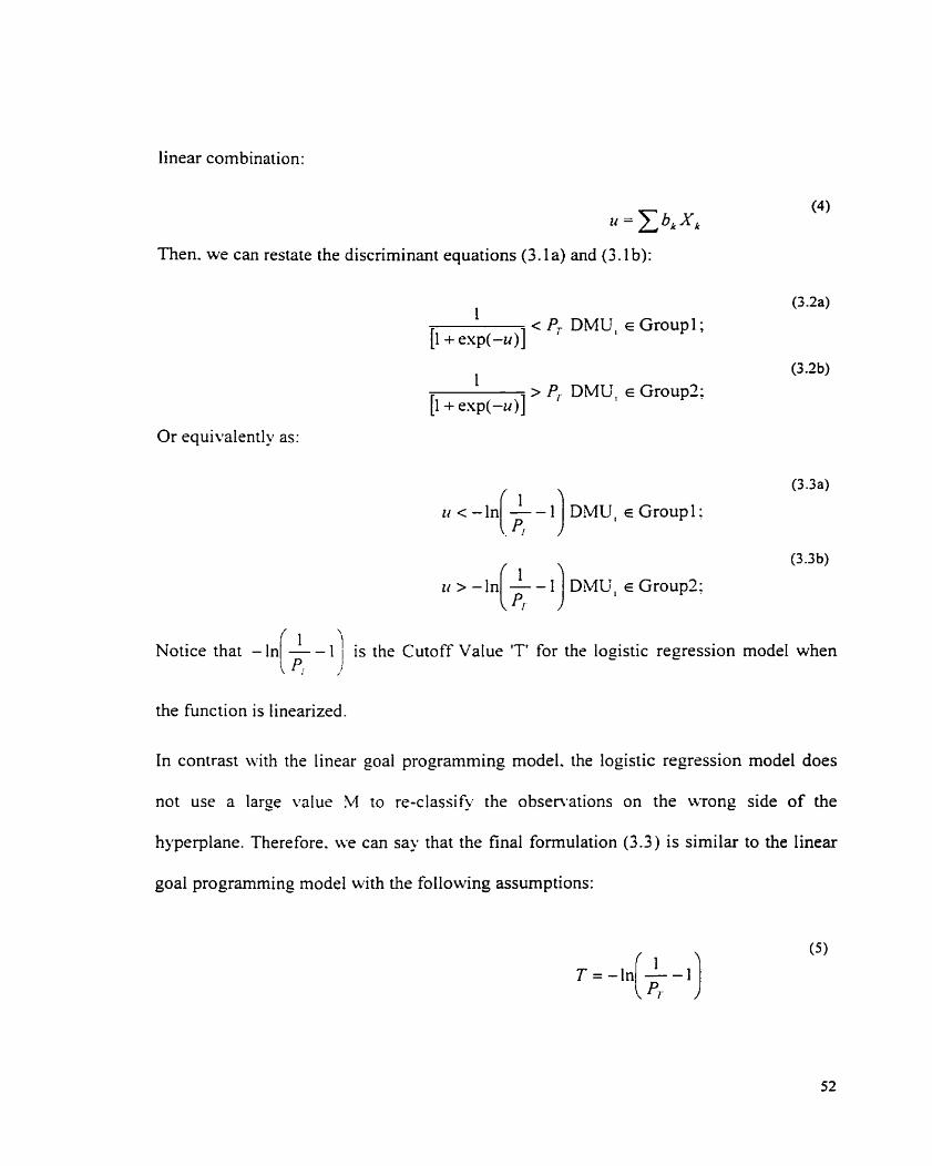
linear combination:

Then. we can restate the discriminant equations (3.1 a) and (3.1 b):

1 < PT DMU, E Group 1 ;

[I + exp(-u)]

1 > P, D M ü , E Group?;

[I + exp(-u)]

Or equivalently as:

t i c - I n / k - l ) DMC, r Groupl:

Notice that - l n - 1) is the Cutoff Value TV for the logistic regression rnodel when ,

the function is linearized.

In contrast with the linear goal prograrnming model. the logistic regression model does

not use a large valus 54 IO te-classify the obsenations on the wrong side of the

hyperplane. Therefore. Lve can say that the final formulation (3.3) is similar to the Iinear

goal prograrnming mode1 with the following assumptions:

And ti = p T ~ -V'X (6)

Assumption (6) is similar to: u = 6, X, = P'Y - v' X. and if we break down the lefi

tem. we obtain: b, X, + b, X, = ,U'Y - lvT .Y where the first summation represents 1 /

the outpurs ( X, = Y ) and the second summation represents the inputs ( X , = X ).

Therefore. this leads to the statement that a solution esists where the positive coefficients

are the p's ( b, = p, ) and the negative coefficients are the v's ( - 6, = v , ).

In conclusion. with the additive DEA mode1 i t appears that the signs of the logistic

regession coefficients can aid in determining the appropriate orientation of the variables:

ci posiri i~ coefficien~ indicales an outpuf and a negorire coefficienf an irrprir.

U'e do not concern ourselves here with significance of ~~ariables in the usual sense.

111.1.2 Data Transformation

In DEA. translation is a means of shifiing the data for some variable. input or output.

This is useful when there are negative numbers present in some of the DMUs for the

variable in question. For the CRS surface. anaiysis results wiIl differ for different

translations. For the VRS surface the sets of efficient and inefficient units remain the

same regardless of the translation. However. efficiency scores may differ for different

translations [90AS].

Scaling is invaluable and a theoretically sound option to use when the matrix is highly ill-

conditioned. Le.. there are very large numbers and very small numbers present in the

matrix. Analysis results for the standard and the non-Archimedian Standard evaluation

systems are not invariant to data scaling. On the other hand, for the invariant and the non-

Archimedian invariant evaluation systems, the results will remain the sarne regardless of

data scaling [95ALS].

A new data set has been included in this study to be used with goal programrning and

integer linear programming computations. This data set is a transformation of the original

data set that has besn provided by the bank. It is a projection ont0 an arbitra- positive

interval (100. 200). resulting in every observation being measured on the same scale

(Figure 111-3). Each variable observation (FTOT. RSP, LOANTOT. MOPCAO.

MDPMTRF. MWDMWPD) has been projected ont0 this scale, by applying the following

transformation:

A is the minimum value of the variable being projected

B is the maximum value of the \mariable being projected

D is the lower boundary of the target scale

E is the upper boundary of the target scale

i is the value of the observation #i before the projection

j is the value of the projected observation #i

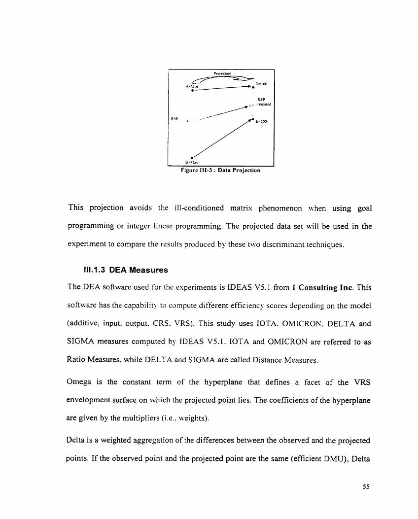
Figure 111-3 : Data Projection

This projection avoids the ill-conditioned matris phenomenon when using goal

prograrnming or integer linear programming. The projected data set will be used in the

experiment to compare the results producrd by these tn-O discriminant techniques.

fll.l.3 DEA Measures

The DEA software used for the espcriments is IDEAS V5.1 from 1 Consulting Inc. This

software has the capabilii? io coinpute diffrrent efficicncy scores depending on the mode1

(additive, input, output. CRS. VRS). This study uses IOTA. OMICRON. DELTA and

SIGMA measures computed by IDEAS V5.l. IOTA and OMICRON are referred to as

Ratio Measures, while DELTA and SIGMA are called Distance Measures.

Omega is the constant term of the hyperplane that defines a facet of the VRS

envelopment surface on ~vhich the projected point lies. The coefficients of the hyperplane

are given by the multipliers (i.e.. weights).

Delta is a weighted aggregation of the differences between the obsenred and the projected

points. If the observed point and the projected point are the sarne (efficient DMU), Delta

will be zero. Delta is optimized for additive models.

Sigma is obtained by weighting the output slack and excess input values by the

corresponding multipliers. For additive models Sigma and Delta are calculated in exactly

the sarne way since the differences between the obsenred and the projected points are

given by the output slack and excess input values.

///.7.3.7 lnput Measures of efficiency

The most standard measure of efficiency in the input-oriented mode1 is Theta, which

represents the proportional reduction of inputs possible in order to obtain the projected

input values. An altematii-e measure is Iota. which is calculated as:

IOZ4 = U R TG2 L O UTP UT + 0.bfEGA

I ÏR TUAL I W UT

The virtual output is calculated by weighting a unit's obsenred output values by the

obtained prices (weights). Similarly. the virtual input is calculated by weighting the

observed input values by the obtained prices. From the following relationship between

Iota and Delta X e can see that Iota is obtained by standardizing the total weighted

distance by the virtual input. Iota is I if and only if the unit is efficient. Le., the observed

point lies on the envelopment surface.

IOTA = 1 - DEL TA VIR TUA L iNP CrT

In summap, both Theta and Iota are measures of input inefficiency. Theta measures only

that portion of the inefficiency that can be realized by a proportional reduction of inputs.

Iota measures the total inefficiency by taking account of both proportional changes in the

factors. and any residual changes needed to get ont0 the frontier.

111.1.3.2 Output Measures of etficiency

The most standard measure of efficiency in the output oriented mode1 is Phi, which

represents that proportional augmentation of outputs possible in order to obtain the

projected output values. An alternative measure is Omicron. which is cakulated as:

0:CfICR Of\' = VIR TUA L IArP UT - OMEGA

WR TUAL OUTPUT

From the follouing relationship between OMICRON and IOTA. we can see that Iota is

obtained by standardizing the total weighted distance between the observed and projected

points b>- the virtual output. Omicron \vil1 be 1 if and only if the unit is efficient.

O M K R o.\- =

Both Phi and Omicron are measures

1 + DELE4 ?//R TUAL OUTP CrT

of output inefficiency. Phi measures only that

portion of the inefficiency that can be realized by a proportional augmentation of outputs.

Omicron measures the total inefficiency in terms of both proportional and residual output

augmentation.

111.2 METHODOLOGY

We wish to test the claim that Our theory that selecting the inputs and the outputs in a

manner consistent wi th expert judgements. can actuall y improve the predictive capability

of DEA models.

The demonstration's aim will be to compare the DEA models thus improved with the

DEA models not built with our method. Two experiments are conducted: one with an

additive orientcd model (the current chapter). and the other with an input oriented model

(the chapter to folloti-).

Each esperirnent will apply the sams msthodology. which consists of: (1 ) determinine an

xerage perforniance of the impro\red DEA modrls and. (2) comparing this average

performance with the set of the other DEA model's performances. The possible number

of DEA models for a given type (i.e. additive or input) corresponds to the set of the

possible combinations of variables: in Our case. there are 728 DEA models (j6 - 1)).

The performance measure of quality that will be used to assess the 'expert DEA" model.

will be that model's ability to classify branches according to their DEA scores. A DEA

mode1 'i' will be considered as bener than a model J' if the model 'i' properly classifies

(consistent with management's judgement ) more branches than the model 3'. We will use

this measure of performance for two main reasons:

We already have classification information provided by the bramh consultants: the

high and low performing branches:

This provides a way to have a unique performance measure for a DEA mode1 and the

scores of the best models (i.e. those that properly classifi the greatest numbers of

branches) are likely to be more easily accepted by branch management.

The average performance computation will be based on the use of a statistical

methodology. Its principle is to calculate a performance that is the average of at least 10

similar experiments' performances. These experiments are similar as they al1 use the same

initial data set. Each experiment builds a predictive model by using 90% of this initial

data set and then testing this mode1 on the 10% left. These subsets are created randomly,

and the result of each predictive mode1 indicates the performance of the corresponding

experiment.

These experiments will also enable us to compare different techniques that help to define

the inputs and outputs (i.e. logistic regression. multiple discriminant analysis. goal

programming and integer linear programming).

To repeat. the rnethodology applied here is based on ten-fold cross-validation [95GD]. Its

principle is as follows: the predictive model is estimated using 90% of the branch subsets

(the analysis sample). and tested on the remaining 10% (the holdout sample). This is done

ten times, each time testing on a different 10%. The average performance on the testing

sets gives an accurate. unbiased estimate of real-world performance (Figure 111-4).

ANALYSE

TEST Y 4

SPLIT n

'redictive Model -

.r\verri_ee performance = estimate of rcal-world performance

Figure I I I 4 : Ten-Fold Cross b'alidation hlethodology

Therefore. the methodolog! used for this experiment is divided into two phases:

The analysis phase. composed of five sequential stages, creates 10 predictive models

using 10 analysis samples:

The predictive phase tests these predictive models on 10 holdout samples.

Figure 111-5 is an illustration of this two-stage approach. Each step is detailed in the next

paragraphs and sarnple results are given.

-10 anaIysis sampIes & 10 holdout sarnples

il/ [ DISCRIMINAST TECHNIQUES

n DEA COMBINATORIAL PROCESS

r w ~ i i r t : hiodrl r

*Logistic tegression. goal programming. multiple discriminant analysis applird to 1 O analysis samplss -Classification Mairices 8: Discriminant Techniques Coefficients

*7280 Additire DE4 cornputaiions ( I O analusis samples x 718 1iO combinations) -10 Classification nbles ( I O malysis samples x DEA measurel

MATCHING DEA SCORES I -Corresponding DE.-\ scores for c x h technique baxd on the signs of the corfficicni

-Cornparison iablr. for rhc DEA mrasure cDrlta) and e x h discriminant technique

.. . - z .

DEA PREDICTIVE CL.L\SSIFICATIOS - - .. . *Cornparison [able for the DEA rneasurr r De11a1 and tach discriminant technique

Figure 111-5 : General Steps For The Additive DEA Experiment

111.3 EXPERIMENT USING AN ADDITIVE DEA MODEL

111.3.1 Estimating the Predictive Model

111.3.1. 7 Random Sampling Stage

The branch consultants have provided a data set of 200 branches. divided into equal parts

of high and low performing branches. (As discussed earlier. the methodology used by the

consultants to categorize branches. is not transparent. but appears to be heavily dependent

on overall sales performance and the demographic makeup of the customer base).

The Random Sarnpling Stage creates I O different subsets of data that are used to build IO

predictive models (Figure 111-6). Each subset is divided into two data sets: The analysis

sample contains 90% of the observations, and the holdout sample. the remaining 10%.

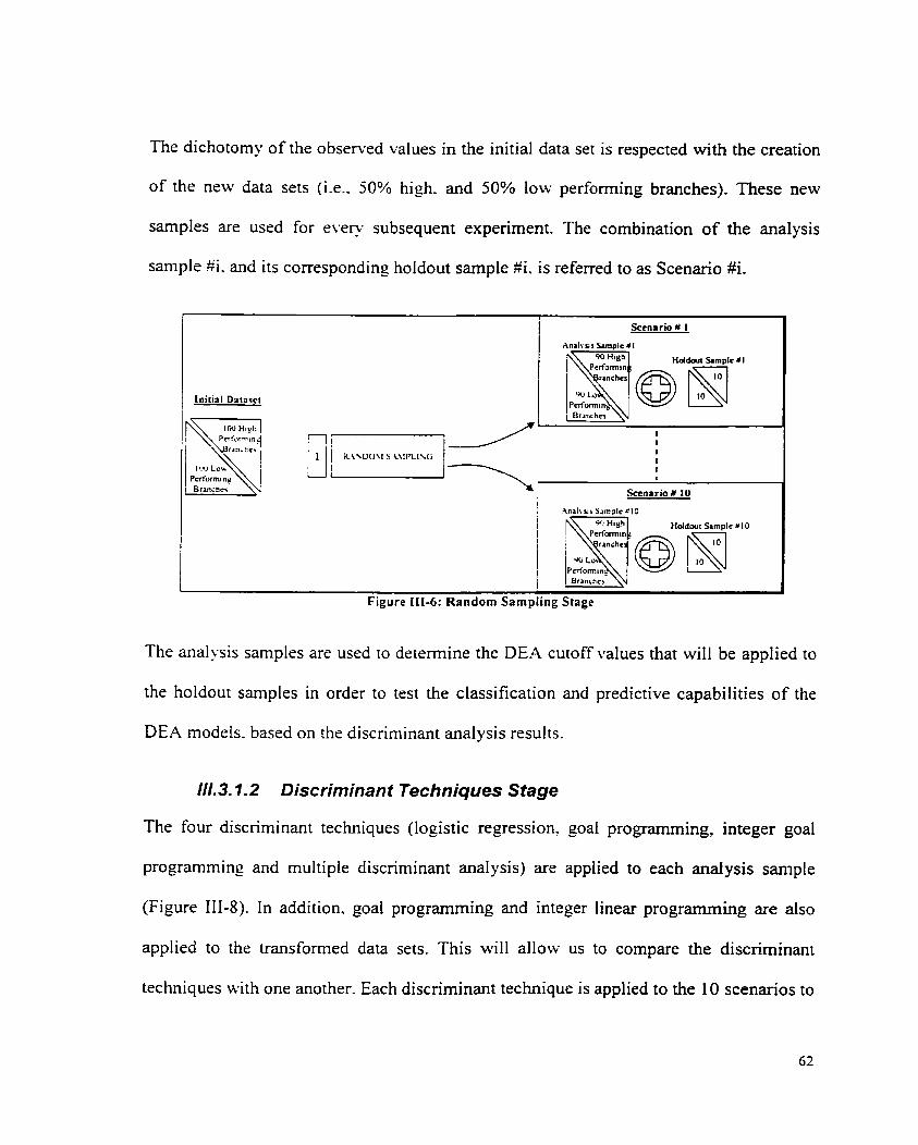
The dichotomy of the observed values in the initial data set is respected with the creation

of the new data sets (i-e.. 50% high. and 50% low performing branches). These new

samples are used for every subsequent experiment. The combination of the analysis

sample fii. and its corresponding holdout sample Xi. is referred to as Scenario #i.

The analysis samples are used to determine the DEA cutoff values that will be applied to

the holdout samples in order to test the classification and predictive capabilities of the

DEA models. based on the discriminant analysis results.

111.3.7.2 Discriminant Techniques Stage

The four discriminant techniques (logistic regression. goal programming, integer goal

programming and multiple discriminant analysis) are applied to each anaiysis sample

(Figure 111-8). In addition. goal programming and integer linear programming are also

applied to the transformed data sets. This will allow us to compare the dis cri min an^

techniques with one another. Each discriminant technique is applied to the 10 scenarios to

obtain the discriminant fünction coefficients.

For example, the logistic regression function for the scenario $1 is:

With (SbkXk) = (3.21 - 2.05*FTOT + 7.3OE-02*RSP + 7.72E-03*L0.4NTOT - 1.52E-

O3*MOPCAO - 6.06E-03*MDPMTRF - 3.96E-05*MWDMWPD).

From this example. and as illustrated by Figure 111-7. we can dcduce that the variables

FTOT. MOPCAO. MDPMTW and MWDMWPD are inputs (their respective logistic

function coefficients are negative) and that RSP and LOANTOT are outputs (their

respective logistic function coefficients are positive).

Variables

0 FTOT

RSP LOANTOT MOPCAO

MDPMTRF MWDMWPD

LR - Coefficients

%f9 -7.05

7.30e-02 7.7-e-02 - 1.52~03

-6.06e-03 -3.96~-05

LR ~ o e K i e n t

S L 5 Nrgativc: Positike Positive

Negativc: Negative N e g a t i ~ e

Inout or e

Input output Ourput

Input Input 1 nput

Figure 111-7: Determining I n p u l And Outputs For Scenario #1 With Logistic Regression (LR)

As displayed in Figure 111-8, each discriminant technique is applied to each of the 10

scenarios in order to produce discriminant functions and thus. the signs of the respective

coefficients.

Scenario # i 4nrlvris Sirnole mi

This proccss 1s rcpeatcd 10 cimes. one for cach scenario

Ferfam~ng ] brancher I

Table 111-2 is an ssarnple of the coefficients cornputed on the 10 scenarios for the Iogistic

regression model. Similar tables for the other discriminant techniques (Le. goal

programming. integer linear programming, multiple discriminant analysis) have not been

displayed here but are available in the appendix.

Table 111-2 : Logistic Regression Sample Results

Scenario #

I 3

-, 2

4

5 6 7 8 -2.03.E-00 7.80E-02 7.35E-02 -1.09E-O3 -3.07E-03 -9.34E-04

FTOT -2.05E-00 -2.09E-00 -2.09E+00 -2.03 E+00 - 1.78E+00 -2.00E+00 - 1.77E-00

RSP 7.30E-02 6.94E-02 8. I7E-02 7.40E-02 4.66E-02 7.59E-02 4.05E-02

LOANTOT 7.72E-02 7.47E-02 7.50E-02 7.62E-02 9.49E-02 7.03E-02 8.83E-02

MOPCAO -1 XE-03 -1.40E-03 - 1.17E-03 - I .52E-03 -2.5 1 E-03 -8.8 1 E-04 -2.3 1 E-03

MDPMTRF -6.06E-03 -4.49E-03 -6.28E-03 -5.6 1 E-03 -9.34E-03 -6.5 1 E-03 -7.52E-03

MWDMWPD -3.96E-05 - 1.98E-04 -3.16E-04 -2.0 1 E-05 1.76E-04

-4.64 E-04 - 1.53E-O4

111.3.1.3 DEA Combinatorial Stage

The DEA Combinatonal Stage computes. for every scenario, and each possible additive

model based on inpuVoutput combinations, a set of tables. called DEA Classification

Tables. These tables are used during the Matching DEA Scores Stage. The DEA

Combinatorial Stage is divided into four steps, repeated 10 times. one for each scenario

(Figure 111-9):

Step 1: Creation of 728 additive DEA rnodels corresponding to the 728 input and

output combinations that are possible with 6 variables.

Step 2: The 728 additive DEA Models are solved. and the DEA measures (for the

additive model it is the DELTA measure) are computed for each DMU.

Step 3: For each scenario and each DEA Mode1 (one pcr input/output combination).

an optimum cutoff value or threshold is computed in order to discriminate as well as

possible among the 180 branches. according to their DEA measures. That is. the

cutoff value is computed so as to maximize the number of branches properly

classified. Thrn. a classification score is computed for each DEA measure that

indicates the number of observations properly classified with the associated cutoff

value. For example. a branch with a DEA score lower than this threshold belongs to

the group 1, otherwise it is classified as being in group 2.

Step 4: The final stage creates the DEA Classification Tables that are used in the

matching process. Each table is composed of 728 rows corresponding to the number

of input/output combinations and. each row gives the optimum threshold and the

number o f branches properly classified for a specific additive DEA mode1 that is

determined by an input/output combination. The classification table is then sorted by

the number of properly classified observations in descending order so the first row

indicates the best combination of inputs and outputs. giving the highest number of

branches properly classified. Consequently, at the end of this process 10 tables are

created (one for each of the 10 scenarios).

Sccnario U i 4 n ~ h sis Samplc =i

This process rs rcpcatrd I O iimcs. one for rach sccnano

l I CRE \TE ' 3 Cmbinrtions o f lnpuud: Oulpuu I

!

7

F I t D T t i k '15 BEbT WREStiOLDS FOR THE DE.* S E A S L R E DELT \

f

/ SORT THE ) L \ l \ I W L E D CL+SSlFlC.\TIO\ TABLE FOR THE DE4 \IEASCRE DELT*

I

1

DEA Classific~rion Table I Delta Additt\c=i I -

Figure 111-9 : DEA Combinatorial Stage (Additive Experiment)

Table 111-3 is an estract of the classification table for Scenario # 1 . The first row indicates

that the best classification score for scenario #1 is obtained by the combination #270 with

163 properly classified branches out of 180.

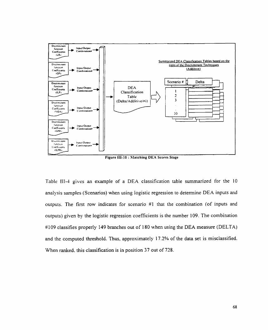
Discnrninani !Lnc:iun

CoctTicr enir in pu^ Ouiput -) Cornbinaiion#

Summîrited DEA Classrfication Tables based on the siens of [he Discriminani Techniaues

{Additive)

DEA Classification

+ Table (Delta/.r\dditi\.e/gi)

Scenario f: Delta 1 kt . , r -

Table 111-4 gives an exarnple of a DEA classification table summarized for the 10

analysis samples (Scenarios) when using logistic regression to determine DEA inputs and

outputs. The first row indicates for scenario #1 that the combination (of inpurs and

ourputs) given by the logistic regression coefficients is the number 109. The combination

#IO9 classifies properly 149 branches out of 180 when using the DEA measure (DELTA)

and the computed threshold. Thus, approximately 17.2% of the data set is misclassified.

When ranked. this classification is in position 37 out of 728.

Table I I I 4 : DEA Classification Table For The Logistic Regression

Similar tables have been obtained for the other discriminant models but have not been

displayed here.

Scenario f:

1 ,

1lL3.1.5 CIassificationSummary Tablestage

This stage summarizes the average ~Iassification measures for every scenario and each

discriminant technique (Figure I I I 4 1 ). Each table created in the previous step is averaged

and reportsd on a row of the resulting summary table. Therefore, one can compare the

performances of the additive DEA mode1 classification capabilities. when assisted by

each discriminant technique.

Summsrrzrd DEA Classification Tables hascd 1 on the siens of ihc Discnminani Techniques

[Addiinci

Position @ Out Of 728 Sorted DEA

Combinations 37

Combination S

1 09

Classification Surnmm Tablr. (Additne) I

1 GPR

# Of Properly Classified Branches Out Of 180

Using DEA Scores (Delta) 149

I 1 - I l

Figure 111-1 1 : Classification Summary Table Stage

% Of Non Properly Classified Branches

1 7.2%

Table 111-5 summarizes the classification results for each discriminant technique. Each

row indicates the average classification results. The first row displays the results

computed when using logistic regression coefficient signs to determine inputs and

outputs. The first column displays the average performance of the DEA models using

these variable combinations to classify branches according to their DEA scores. The

second coiumn indicates the percentage of branches that are misclassified. The final

colurnn shows the average r d of this score within the DEA Classification Tables. For

example, the DEA Score of 136. in the first row, means that when using the logistic

regression coefficients and the Delta measure (additive DEA score). 136 branches out of

180 are properly classified on a\-erage. meaning that 24.4% of the branches are

misclassified. This rrsult is. on al-erage. in the 78.~'~ position (out of 728) within the

DEA Classification Table. The last row shows the best results: in this case it indicates

that determining inputs and outputs with goal prograrnrning is the best method for

computing DEA scores in terms of cIassifying the branches in the best manner (the best

results are underlined). I r is noted that re-scaling the original data gives the same results

when using goal programming.

Table 111-5 : Summarized DEA Classification Table (Additive ModelIAnalysis Stage)

Average Results Of The

1 10 Scenarios

Discriminant Technique Lis

Inputs and Outputs selected with LR coefficient signs

Inputs and Outputs selected with GP

Inputs and Outputs selected wirh GP coefficient signs (Data Rescaled)

Inputs and Outputs selected with ILP coefficient signs

Inputs and Outputs selected with ILP coefficient signs (Data rescaled)

Inputs and Outputs selected with MDA coe ficient signs

--

Best Results

111.3.2 Testing the Predictive Model

111.3.2.7 DEA Predictive Classification Stage

The DEA Predictive Classification Stage is the second part of the methodology. The

principle is to use the same combinations of inputs and outputs. and the same thresholds

as those computed in the analysis part. This predictive process is divided into three steps

(Figure III- 12):

Ranking Out Of 728 Sorted DEA Combinations

# Of Properiy Clissified DMUs Out Of 180 Using DEA Scores

Step 1: The DEA Predictive Process cornputes the DEA scores for each possible

combination of inputs and outputs (728 combinations). Note that we do not compute

DEA scores on just the holdout samples, but on the entire data set composed of 200

branches. By using the thresholds and the coefficients computed in the previous part,

we create 10 DEA classification tables.

Oh Of Not Properly Clarsified DMUs

Step 2: The Matching DEA Scores Process is sirnilar to the one applied during the

analysis part. It consists of building one table per discriminant technique, indicating

for each scenario the classification score that corresponds to the combination of input

and output computed during the analysis phase.

Step 3: The Classification Sumrnary Tables Process is the final stage that sumrnarizes

the measures for the 10 scenarios and the discriminant techniques into one table.

IO ho1 Jout sainplrs

I \ *Classification Matrices & Discriminant Technique Coefficients

DE.4 PREDlCTIL'E PROCESS 0728 Additive DEA computations t :\ddiii\r. Xlodr.1 I IO Classific~iion tablcs ( I O holdout samplcs s DEA rneasurc)

SIATCH I S G DEA SCORES *Conesponding DEA scores for rach technique basrd on the signs of the cositicicnt

*Cornparison table tor thc DEA measure (Delta) and each discriminani technique

Figure 111-12 : DEA Predictive Classification Stage

The DEA Predicti\,e Procsss is similar to that of the analysis part. but it is slightly

different in a feu. aspects:

The data set is composed of 200 branches. Indeed. the DEA is nin on the 200

observations and not only on the 20 observations of the holdout sample. Uniike some

statistical tools. DEA is a relative benchmarking tool? which means that the set of best

practices is based on the full set of DMUs. Each time a new DMU is included in the

sarnple. the set of best practices and the efficient frontier have to be recomputed. If

the efficient frontier is modified, then some DMUs that were efficient before c m

become inefficient and have their DEA score modified. therefore impacting the final

classification. I f we had to use only the 20 DMUs we would forget the previous

branches and their efficient frontier. and would build another efficient frontier taking

into account only these 20 DMUs. Figure 111-13 illustrates this idea with a small

sample of 7 DMUs. The graph on the top plots the 7 DMUs and their efficient

frontier. One can observe, with the two graphs belou that use two subsets (cal1 them

analysis and predictive sets), different results. and most imponantly. changes in the

efficient frontier result;

The combinations of inputs and outputs used to select the corresponding DEA mode1

during the Matching DEA Scores stage. are identical to those of the analysis pan:

The DE.4 thresholds are identical to those of the analysis part.

Complerc Vs fanial DEA Anal' sss

- - - - - -- . - - - - - -

Figure 111-13 : Complete Vs Partial DEA Analyses

As shown in Figure 111-14. the principle is to:

Create 728 combinations of inputs and outputs:

Compute the 728 additive DEA models composed of 200 branches each (instead of

180 branches during the analysis phase);

Classify the 728 samples using the thresholds computed in the previous analysis

stage. for each of the 1 O scenarios.

The final DEA classification tables (10 tables) are then sorted, in descending order-

according to the numbers of branches properly classified.

i Initial Dataset

I I CRE.4TE 728 Combinations of Inputs d Output3 I RCX 728 DE4 ADDITI\'E \IODELS

CLXSSIFl. THE 728 HOLDOL T SAifPLES CSIYG THE ASALYSIS SAX1PLES THREHOLDS FOR THE DEA XIEASLi'RE

DELT.4. 1

SORT THE SC%IXIAiüZED CLASSIFICATIO\ TABLE FOR THE DE.4 MEASCRE DELT.4

1 DEA Classiftcrition Table 1 1 1

Thcse stcps are repea~ed 10 times. one for each scenario

Figure 111-14 : DEA Predictive Stage

The 10 DEA classification tables are then used to match the ciassification scores for each

scenario and each discriminant technique, with the combination of inputs and outputs

determined by the discriminant fùnction coefficients computed in the previous parts.

Figure 111-1 5 illustrates this process that builds the surnrnary tables in a manner similar to

that in the analysis part.

Input Output C ~ b i n u i o n = + i Sumrnanzcd DEA ClassitÏcai~on Tables bascd on the

sicns o f ihe Dtscnrninmr Tcchnioiics f Addit~vrr

r i Scenario $

l 1

i 1. IILPR)

Figure 111-15 : Matching DEA Scores Stage

The final stage (Figure 111-1 6) sumrnarizes the average classification measures for every

scenario and each discriminant technique. Each table created in the previous step is

averaged and reported on a row of the resulting summary table. Therefore, one can

compare the performances of the DEA dassification measure and each discnminant

technique.

Summarizrd DEA Classitication Tables based on the siens o f the Discriminant Techniaues

! Additive) Classificarion Surnmarv Table

[Additive)

1 Delta 1

ILP

Figure 111-16 : Classification Summary Table Stage

Table 111-6 shows the classification resuits obtained at the end of this process. Each row

indicates the average classification results. The first row displays the results computed

when using logistic regression coefficient signs to determine inputs and outputs. For

example. the DEA Score of 160.5. in the second row, means that when using goal

programming coefficients and the Delta measure (additive DEA score). 160.5 branches

out of 200 are properiy classified on average, which is similar to saying that 19.8% of the

branches are misclassified. This result is, on average. in the 46.jth position (out of 728)

within the DEA Classification Table. The last row shows the best results. Again. it would

appear that goal programming is the best technique for selecting variables for computing

DEA scores. in that it classifies the branches in the best manner (the best results are

underlined). Specifically. goal prograrnming appears to be a favorable vehicle for

incorporating expert opinions into the DEA framework

Table 111-6 : Summarized DEA Classification Table (Additive Model/Predictive Stage)

This chapter has concentrated on the additive model for DEA. In the following chapter

the same ideas are revisited. but in the contest of the input-oriented model.

Ranking Out Of 728 Sorted DEA Corn binations

7 5

- 46.5

- 46.5

206

76

76

46.5

O h Of Not Properly Classified DMUs

24.0%

- 19.8%

19.8%

3 1 .O%

25.3%

25.3%

19.8%

Average Resuits Of The # OC Properiy 10 Scenarios Classified DMUs

Out OC 200 Using DEA Scores

Inputs and Outputs selected with LR coefficient signs

Inputs and Outputs selected with GP coefficient signs

Inputs and Outputs setected with GP coeficient signs (Data Rescaled)

Inputs and Outputs selected with ILP coefficient signs

Inputs and Outputs selected with ILP coefficient signs (Data rescaled)

Inputs and Outputs selected with iLLD.4 coefficient signs

Best Results

152

- 160.5

- 160.5

138

149.5

149.5

160.5

IV. EMBEDDING EXPERT KNOWLEDGE IN THE INPUT- ORIENTED DEA MODEL

I V . INTRODUCTION

In this chapter we use the input-oriented DEA Model. and run the same experiments as

those of the previous chapter. Recall that the input onented (VRS) formulation is

expressed by:

Except for the mode1 orientation, the scope and assumptions of the esperiment are

essentially the same.

A data set of 200 branches with the sarne generated analysis and holdout samples:

The sis \variables FTETOT, RSP. LOANTOT. MOPCAO. MDPMTRF and

MWDMUPD;

The use of the ten-fold cross validation methodology;

The discriminant techniques are not dependent on the DEA mode1 orientation. hence.

the discriminant function coefficients found earlier are reused here;

The sarne transformed data to be used with goal programming and integer linear

programming (re-scaled data set) apply here;

The DEA measure to classify the bank branches is now the input measure IOTA;

The principle to select the sets of inputs and outputs is based on the signs of the

discriminant function coefficients (a negative coefficient indicates an input variable

and a positive coeff~cient indicates an output variable).

1V.2 EXPERIMENT USlNG AN INPUT-ORIENTED DEA MODEL

IV.2.1 Estirnating the Predictive Model

The methodology used for this experiment follows the same principles as that used with

the additive rnodel. and is divided into tn-O phases (Figure IV-1):

The analysis part. composed of three sequential stages, creates 10 predictive models.

usine 10 analysis samples already created during the previous experiment.

The predictive pan tests rhese predictive models on 10 holdout sarnples. also created

during the previous esperiment. Notice that we do not have to regenerate the 10

scenarios. and do not cornpute the discriminant function coefficients again. These

steps have already been done ~vith the additive esperiment.

-16 analysis wmplcs 8: I O holdout urnples

\ *Classification Maaices B: Discnrninani Technique Coefficients

DE* COblJ3lsAToRIAL PlKXESS 1 -7280 Input DEA mpuiations ( l O anal? SIS wmplrr \ 728 1, O (Input hfodcl ) carnbinaiions)

n 10 Clamfication tabla ( 10 andysis sampla x DEA meaurc)

-

121 LLATCHING DEA SCORES .Corresponding DEA xorcs for cach techique baxd an the si- of the cocfficicni

n u CLASSIFiC.4TION SUhUURY TABLE *Cornpanson table for ihc DEA rnczure (lofa) and cach

drxnrninani icchnique

Figure IV-1: General Steps For The Input DEA Experirnent

The DEA Combinatorial Stage cornputes a set of classification tables for every scenario,

and each possible input-oriented DEA model. based on input/output combinations. These

tables are used dunng the Matching DEA Scores Stage. This process is similar to the one

in the previous chapter and creates. therefore. 10 sorted classification tables summarizing,

for each combination. the best threshold and the number of properly classified branches.

Table IV- 1 is an extract of the classification table for Scenario # 1. The first row indicates

that the best classification score for scenario #1 is obtained by the combination #133 with

175 properly classified branches out of 180.

Table IV-1: DEA Classification Table For Scenario # I (Out Of 10)

SimiIar to the prei-ious chapter. during the Matching

table per discriminant technique.

Input DEA Model

DEA Scores

Combination # Out Of 728

133 135 216 422 43 2

Stage. we create one

Table IV-2 gives an exarnple of a DEA classification table sumrnarized for the 10

analysis samples (scenarios). when using logistic regression to determine DEA inputs and

outputs. The first row indicates. for scenax-io #1' that the combination (of inputs and

Threshold

0.39976 0.3 1492 O. 13589 0.3 128 1 0.377 13

outputs). given by the Iogistic regression coefficients, is the number

combination #IO9 classifies properly 159 branches out of 180 when using

109. The

the DEA

# Of Properly Classified Branches Out Of 180

175 1 74 173 173 173

measure (IOTA) and the computed threshold, meaning that 11.7% of the data set is

misclassified. When ranked. this classification is in position 63 out of 728. SimiIar tables

have been obtained for the other discriminant models but have not been displayed here.

# Of Not Properly Classified Branches Out Of 180

5 6 7 7 7

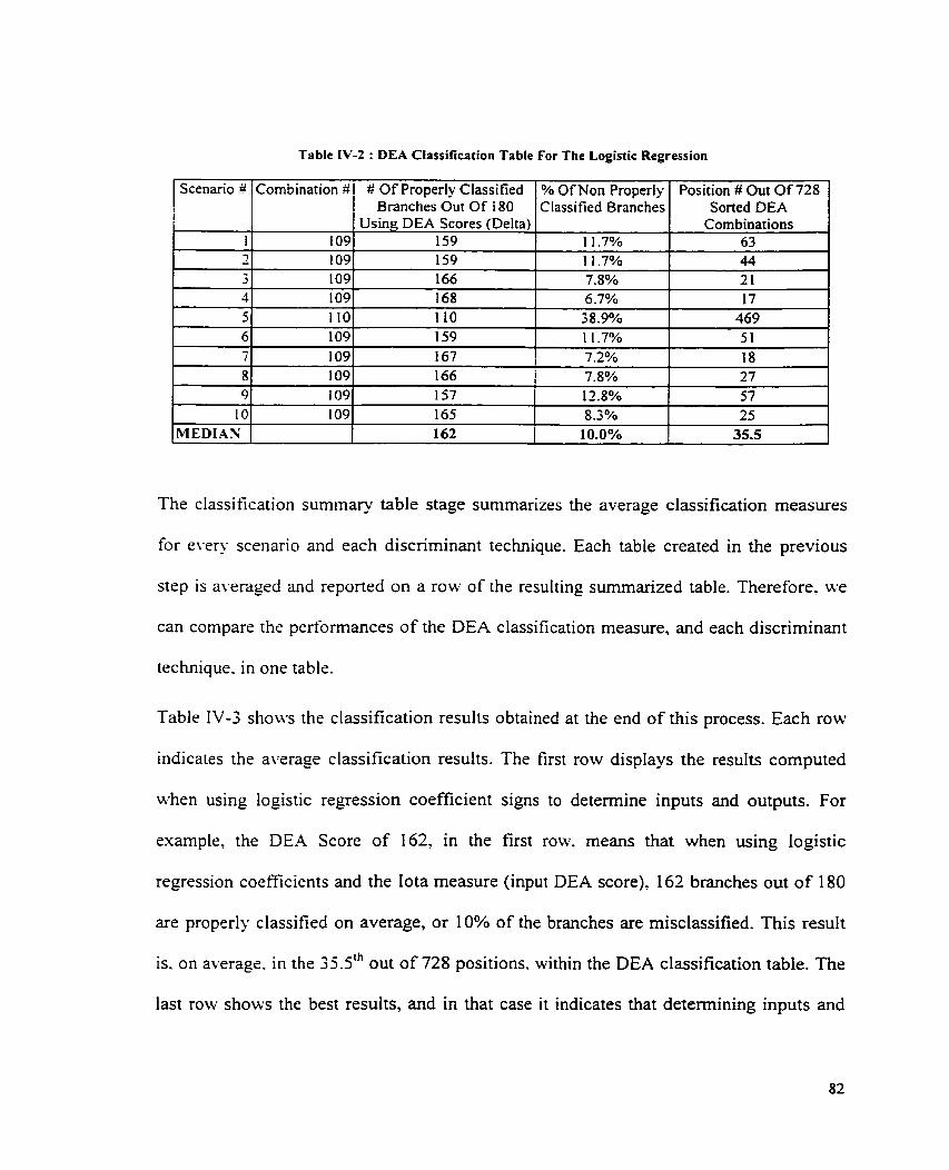
Table IV-2 : DEA Classification Table For The Logistic Regression

Scenario ii

The classification summary table stage summarizes the average classification measures

! Usinp DEA Scores (Delta) i 159

159 166 168 110 159

for ever). scenario and each discriminant technique. Each table created in the previous

Combination

step is averaged and rsported on a row of the resulting summarized table. Therefore. we

I I .y'/0 1 1.7% 7.8% 6.7%

38.9% 1 1.7%

can compare the performances of the DEA classification measure, and each discriminant

# Of Properly Classified Branches Out Of 180

Combinations 63 44 21 17

469 5 1

technique. in one table.

Table I V 4 shows the classification results obtained at the end of this process. Each row

% Of Non Properly Classified Branches

indicates the average classification results. The first row displays the results computed

Position # Out Of 728 Sorted DEA

when using logistic regression coefficient signs to detemine inputs and outputs. For

example. the DEA Score of 162, in the first row. rneans that when using logistic

regression coefficients and the Iota measure (input DEA score), 162 branches out of 180

are properly classified on average, or 10% of the branches are misclassified. This result

is. on average. in the 3 5 S t h out of 728 positions. within the DEA classification table. The

last row shows the best results, and in that case it indicates that determining inputs and

outputs with logistic regression is the best technique for computing DEA scores; it

classifies the branches in the best manner (the best results are underlined).

Table IV-3: Summarized DEA Classification Table (Input DEA ModeVAnalysis Stage)

Average Results Of The # Of Properfy 10 Scenarios Classified DMu's

Out Of 180 Using DEA Scores

Inputs and Outputs selected with LR 162 - coeficient signs

Inputs and Outputs selected with GP coeficient signs

Inputs and Outputs selected with GP

156

156 coefficient signs (Data Rescaled)

Inputs and Outputs selected with ILP coefficient signs

Best Results 1 162

146

Inputs and Ourputs selscted \vitIl ILP coeficient signs (Data rescaled)

Inputs and Outputs seIected with MDA coefic ient signs

159

133.5

IV.2.2 Testing the Predictive Model

This DEA Predictive Classification Stage is similar to the one applied in the previous

chapter. The principle is to use the same combinations of inputs and outputs and the same

thresholds as those compured in the analysis stage. This predictive process creates a final

table summarizing the average classification measures for every scenario, and each

discriminant technique. Therefore. we c m compare the performances of the DEA

classification measure, and each discriminant technique in a single table.

Table IV-4 summarizes the average classification measures for each scenario and

.- -

Oh Of Not properly Classified DMUs

- - - . . . -

- Ranking o u t Of 728 Sorted DEA Combinations

discriminant technique. We note as wel1 in this case that the recommended discriminant

tool for selecting inputs and the outputs is logistic regression. Indeed. it is with this

technique that we obtain the best average results: 182.5 branches out of 200 are properly

ciassi fied.

Other techniques such as goal prograrnrning (GP) and integer linear prograrnming (ILP)

also perform well: 180 branches are properly classified when using ILP to select inputs

and outputs. and 17 1 branches are properly classified when using GP.

Table IV-4: Surnrnarized DEA Classification Table (Input DEA ModeWredictive Stage)

coefficient signs (Data rescaled ) 1 1 1 1

Ranking Out Of 728 Sorted DEA Corn binations

26.5

62.5

62.5

120

Inputs and Outputs selected with ILP 1 l 801 1 O.oO!l 321

O h Of Not Properly Classified DMUs

8.8 O/%

14.5%

14.5%

1 8.590

Average Results Of The # Of Properly 10 Scenarios Classified DMUs

Out O f 200 Using DEA Scores

Inputs and Outputs selected with hfDA coefficient signs

Inputs and Ourputs seIected \vith LR coefficient signs

Inputs and Outputs selected with GP coefficient signs

Inputs and Outputs selected with GP coeficient signs (Data Rescaled)

Inputs and Outputs selected with ILP coefficient signs

Best Results

182.5-

171

171

163

153.5

182.5

23.3% 179

8.8% 26.5

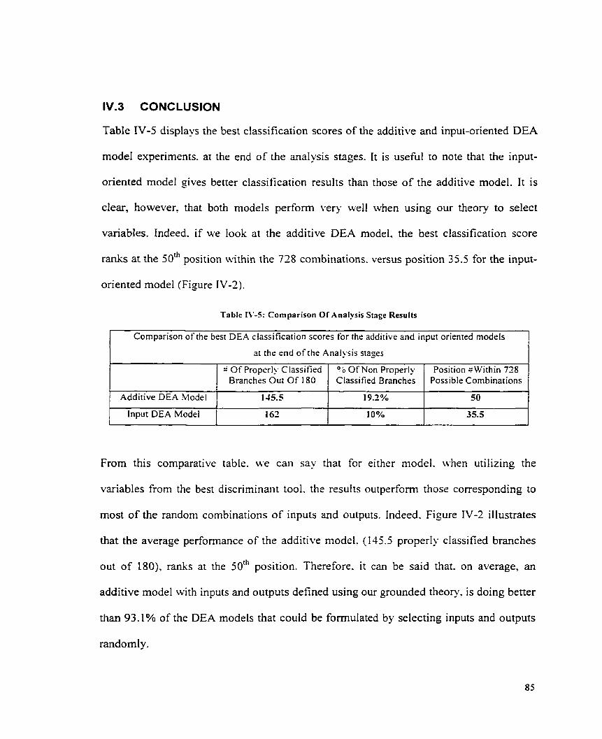
IV.3 CONCLUSION

Table IV-5 displays the best classification scores of the additive and input-oriented DEA

mode1 experiments. at the end of the analysis stages. It is useful to note that the input-

oriented model gives better classification results than those of the additive model. It is

clear, however. that both models perform very well when using Our theory to select

variables. Indeed. if we look at the additive DEA model. the best classification score

r a d s at the 50'~ position within the 728 combinations. versus position 35.5 for the input-

oriented model (Figure IV-2).

Table 1\'-5: Comparison Of Analysis Stage Results

Comparison of the best DEA classification scores for the additive and input orienred models

l at the end o f the Analysis stages l C

= Of Properly Classified Branches Out Of 1 80

I I I

From this comparative table. u-e can say that for either model. when utilizing the

Additive DEA Model [ 145.5

Input DEA Model

variables from the best discriminant tool. the results outperfom those corresponding to

9'0 Of Non Properly Classified Branches

most of the random combinations of inputs and outputs. Indeed. Figure IV-2 illustrates

Position =Within 738 Possible Combinations

1 9.Z0/U

162

that the average performance of the additive model. (145.5 properly classified branches

out of 180), ranks at the 5oth position. Therefore. it can be said that. on average, an

50

additive model with inputs and outputs defined using our grounded theory. is doing better

10%

than 93.1 % of the DEA models that could be formulated by selecting inputs and outputs

35.5

randornly.

Xots as well that the first DEA model classifies 166.6 branches out of 180 and the last

DEA model classifies 91 -3 branches out of 180.

Sorrcd DEA Clustficaiion Scores AT-]

Lasr DEA combination 9 1 2 out of 180 L I

Figure IV-2: Illustration Of Ranking DEA Results (Additive ModellAnalysis St

Table IV-6 displays the best classification scores of the additive DEA model and the

input-oriented DEA model experiments. at the end of the predictive stages. Here again.

we can see that the classification results are impressive.

Table IV-6: Comparison Of Predictive Stage Results

I I I

Input DEA Model 1 182.5 8.8% 1 26.5 1

Comparison of the best DEA classification scores for the additive and input oriented rnodels at the end of the predictive stages

These average performances demonstrate that the method to select DEA variable

Additive DEA Model

orientations, based on the sign of the discriminant function coefficients, performs well.

One can see from Figure IV-3 that in the predictive stage. the average DEA performance

86

;: Of Properly Classified Branches Out Of 200

160.5

% Of Non Properly Classified Branches

19.8%

Position fi Within 728 Possible Combinations

46.5

for the additive model ranks at the 46.sth position. The results for the input-oriented

model are even better: 182.5 branches out of 200 are properly classified, and it ranks at

position $26.5.

Soned DEA Classdcmon ~ c u r e s ) ~ ~

Bcst ALerage DEA score 183 9 oiii of 200 + Avengc DEA performance 160 5 out o f 200

1 1 Figure I\'-3: Illustration Of Ranking DEA Results (Additive hlodel/Predictive Stage)

In addition. Table IV-4 shows that goal programrning is essentially as good as logistic

regression (see resuits with ILP Input Re-scaled) or other discriminant techniques in

selrcting \pariables.

IV.3.1 Classification of holdout samples

As seen previously, because of the nature of DEA, which is a relative benchmarking tool, the results in the Predictive Stage Vary slightly from those of the Analysis Stage. Indeed, the models computed during the Analysis

Stages have been applied on the whole data set (200 DhIUs), instead of being applied sirnpIy on the hoidout sample (20 DMUs). Although our approach does not change the demonstration, (the purpose was to compare DEA models thus improved), we extracted the holdout samples from the experiments and have displayed the

results in Table IV-7 and Table IV-8.

These two tables show. for the 10 scenarios, the classification results when using goal

prograrnrning coefficient signs to determine inputs and outputs. Similar tables have been

obtained when using other discriminant techniques (LR. ILP, MDA), but have not been

presented here.

During the Analysis Stages (using 180 DMUs). we built DEA models that have been

tested on the remaining 20 DMUs (using the thresholds computed in the previous step).

The first table displays the results for the additive experiments. One can see that, on

average. 18.5% of DMUs out of 20 are not properly classified. meaning that 16.3

branches out of 20 are properly classified. The second table displays the results for the

input esperiments. i.e. 16.5% of DMUs out of 20 are not properly classified or 16.7

branches out of 20 are properly classified.

These results illustrate the predictiïe capability of the DEA models thus obtained.

although the main objective is to demonstrate the superiority of such models compared to

other DE.4 models built randoml~,.

Table IV-7 : Classification Of Holdout Sarnples Using Additive DEA Models And Goal Programming Coefficient S i ~ n s To Select Inputs And Outputs

Holdout Samples

1 7 -

1 O 1 0.4578 Average

Threshold

0.592 13 0.58852

16 16.3

20.0% 18.5%

# of properly classified DMUs Out Of 20 Using DEA Scores

17 18

O/O Of Not Properly Classisifed DMUs

1 5.0% 1 O. 0%

Table IV-8 : Classification Of Holdout Sarnples Using Input DEA Models And Goal Programrning Coefficient Signs TO Select inputs And Outputs

- -

[ Holdout 1 Threshold l# of properly classified DMUs Out 0 d O/O Of Not Properly 1

I

Average 1 16.7 1 16.5% 1

Sarnples I 9 -

IV.3.2 Cases with predefined Input and Output variables

The branch consultant kno~vledge ussd for these experiments is the classification of

branches into two groups: the high and low performing branches. One can also take into

account another type of information such as predefined variable orientations. Indeed. in

man! cases. the brancl~ consultants. when classifying branches. already know which

variables are definitely inputs and which are outputs, versus those that can be considered

as eiihev inprtrs or ourprtrs. It is important to consider this kind of information during the

anal ysis.

In Our case. the branch consultants were requested to specify which variables they would

consider as inputs and which as outputs. They defined FTETOT as being an input and

RSP and LOANTOT as being outputs (Table IV-IO). They displayed no strong opinion

about the remaining variables. We refer to these as "flexible" variables.

0.592 13 0.58852

. -

20 &ing DEA Scores 16 16

Classisifed DMUS 20.090 20.0°/0

Table I\'-IO: Variable Predefined Orientations

Variable

FTETOT

Orientation

RSP

Description

I

LOANTOT

INPUT

OUTPUT

MOPCAO

the sum of al1 fidl time employees (sales and service positions)

The number of retirement savings plans sold

OUTPUT

I 1

Therefore. this type of information can be incorporated into the rnodels by matching the

signs of the coefficients according to their predefined orientations. For instance. FTETOT

is defined as an input. which rnsans that its associated coefficient. nithin any

discriminant model. should be nepative. Similarly. an output variable indicates a positive

coefficient.

the total of al1 loans and niongages

Flexible

MDPMTRF

MWDMUPD

There is no con\.enient mechanism for adding this kind of constraint to models such as

logistic regression or multiple discriminant analysis. whereas this can be done with goal

programming rnodels. Fortunately. as discovered earlier. goaI programming provides

results that are approximately on par with logistic regression. Hence. there is no sacrifice

in discriminant ponrer. by resorting to goal prograrnming as the tool of choice. Therefore,

adding sign restriction constraints ((3) and (4) in the model below) to the previous integer

goaI programming structure results in the following formulation:

the total of accounts opened

Flesible 1 the number of deposits and transfers I

Flexible the number of withdra~vals and updates

Minimize y ,

subject to :

(1)A,x - My, c b - E i E Gl

( 2 ) A , x + M y , > b + ~ i e G ,

( 3 ) x , > O k E (RSP. LOANTOT } ( 4 ) ~ , < O z E {FTETOT } ( 9 7 , E {oJ} (6)b unrestrict ed in sign

(7)s, unrestrict ed in sign

Notice that one could also use Glover's Models by imposing the same additional

constraints. (3) and (4). The principle is to cany out the sarne experiments as those of the

previous chapters. but with three main differences:

We use only one discriminant technique. integer linear programming. to determine

the orientation of the "flexible" variables. and compare the results with those of the

corresponding non- resrncted DEA models (i.e. additive and input experiments);

Additional goal programming constraints are imposed on the integer model. This is to

take into account the fact that RSP and LOANTOT are outputs and that FTETOT is

an input.

The number of possible inputloutput combinations is reduced because 3 variable

orientations are now known; there are now 27 combinations.

RSP & LOAhTOT

A ncgau\c coefficient indicare, an Input flOrtsnrarions 4 p o s i u ~ c c o c ~ c r e n i indicatcr an output

FTETOT RSP. LOASTOT. \tDPVTRF

1 PE.4 \li>dcl

Figure IV-4: Restricting M'eights Of Goal Programming ,Mode1

According to the branch consultant strategy. some input and output combinations will not

be possible rven if the? are included in the 27 remaining cases. Indeed, if one looks at

Table IV-12, it can be seen that the first row indicates the combination #135 that

corresponds to the following variable combinations: one input (FTETOT). tw-o outputs

(RSP and LO.ANTOT). with the other variables are not considered for the analysis.

Recall that the strategy is to keep al1 variables within the analysis scope to be able later

on to reduce inputs or increase outputs of the inefficient branches to bring them to the

efficient frontier. Therefore. the ranking will be based on the remaining combinations.

Table IV-1 2 displays for one of the ten scenarios (i.e. scenario #1), the input and output

combinations and the classification results for each of the 27 possible combinations. The

values in this table are sorted. in descending order. according to the number of properly

classified branches. The best DEA mode1 (in terms of classification capability) is in first

position. and the worst is in last position. Similar tables have been obtained for the other

scenarios, but have not been displayed here. Each row of this table specifies:

Its input and output combination number.

Its input and output combination description. A value of 1 defines an input, a value of

2 an output. and a value of 3 indicates that the variable is not included in the analysis.

The last value is used for the durnmy variable. Recall that this variabIe has been

defined to help us work with pure input and pure output cases. For instance. the

combination #IO9 indicates the following inputs and outputs for the flexible

variables:

1 FTETOT 1 1 1 INPUT 1 ~redefined

Variable Combination Id

RSP

LOANTOT

Orientation

2

MOPCAO

MDPMTRF

The computed DEA threshold to discriminate the branches.

Comment

- 3

MWDMUPD

The number of properly classified branches. using this input and output combination

and this DEA threshold:

OUTPUT

I

1

The number of non-properly classified branches.

Predefined

OUTPUT Predefined

INPUT

INPUT

Flexible I

Flexible

Flexible

INPUT

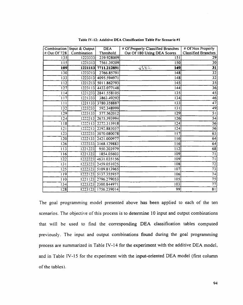
Table I\'-12: Additive DEA Classification Table For Scenario # t

( Combination 1 Input &: Output # Out Of 728 Combination

135 1223333

DEA # Of Properly Classified Branches # Of Non Properly Threshold Out Of 180 Using DEA Scores Classified Branches 239.928009 15 t 29

The goal programming model presented above has been applied to each of the ten

scenarios. The objecti\.e of this process is to determine 10 input and output combinations

that will br used to find the corresponding DEA classification tables computed

previousl~.. The input and output combinations found during the goal programming

process are summarized in Table IV-14 for the experiment with the additive DEA model.

and in Table IV-] 5 for the esperiment with the input-oriented DEA model (first colurnn

of the tables).

Table IV4 1 displays the classification table for the experiment with the input-oriented

DEA models, and the scenario #1. Similar tables have been obtained for the other

scenarios, but have not been dispIayed here.

Table IV-1 1: Input DEA Classification Table For Scenario #1

Combination Input & Output DEA d Of Properly Classified Branches f; 0 f ~ o n Properly f: out of 728 Combination Threshold Out Of 180 Using DEA Scores Classified Branches

135 1223333 0.20576 179 I 1 09 122 1 1 13 0.28851 165 15 130 12232 13 0.3266 1 154 26 132 322323 3 0.40456 151 29

The 27 input and output combinations are sorted by the number of branches properly

classified in descending order. Combination #109 is in the second position in the table.

This means that a goal programming model, with additional constraints imposed, that

determine which of the flexible variables are inputs and outputs. helps in defining a DEA

model that is doing better than any of the 25 remaining models.

In addition, if we consider that. in accordance with bank consultants' strategy. we want to

keep every variable in the analysis, combination #IO9 is in first position. Indeed.

combination # 135 should be escluded from the analysis set since the remaining "flexible"

variables are not included in the analysis (they are neither inputs nor outputs).

Table IV- 14 and Table IV- 1 5 display sumrnaries of the experiments of the additive and

input-oriented DE.4 models. The ten-fold cross validation methodology has been used to

compute an average performance for the restricted models in each orientation. Each table

has 10 rows. one for each subset of 180 branches. Each subset is used in the goal

programming restricted model to find the inputloutput combination. In that case.

combination HO9 is chosen for every scenario (it could be different for some of them).

Each row. then. indicates the number of branches properly classified. and the percentage

of branches not properly classified. when using the DEA scores computed by the model.

(additive or input). that corresponds to the inputs and outputs defined by combination

8109. The last column displays the ranking of each scenario. within the 27 sorted possible

combinations (Table IV- 12). Notice that the ranking does not esclude the scenarios with

variables excluded (such as the scenario # I 35).

Table iV-lit: Averaged Additive DEA Classification Results For The 10 Scenarios

Classification Results # Of Properly Classified O h Of Not Properiy Ranking Out Of 27 1 DMUs Out Of 180 Using Classified DMUs Sorted DEA

DEA Scores Corn binations l

In conclusion. restrictions impossd on the goal programming mode1 multipliers. to

express variable orientations predefïned by bank consultants. provides better results. on

average. than is true of the umestricted DEA version. Recall that the average

performance of the additive esperiinent gak-e 145.5 branches properly classified while the

average restricted result is 147.1 branches properly classified.

Table IV-1 5 demonstrates the same conclusion u-ith the input experiment: the

unrestricted version computed an average performance of 162 properly ciassified

branches. while the fised sign mode1 computed an average of 164.5 branches out of 180

properI y classi fied.

Table IV-15: Averaged Input DEA Classification Results For The 10 Scenarios

Classification Results 1 # Of Properly Clauified 1 O h Of Not Property 1 Ranking Out Of 27

I DMUs Out Of 180 Using Classified DMUs DEA Scores I Combinations I DEA

- -

I Average 8.6% 2.1

Combination # for the 10 ~ c e n à ; i o S \ . 1 09 165 8.3 % 2

V. MODEL EXTENSIONS

V.1 DEA MODEL ENHANCEMENT- EXPERT OPINION CONSTRAINTS

V.1.l Imposing Goal Programming Constraints within an Additive DEA Model

The model structures discussed above build expert opinion into the firsr stage of the

analysis. where classification models are applied to decide variable designation (inputs

and outputs). In the second stage. a standard DEA model is used to derive performance

scores for the DMUs. Arguably. the performance measures can be enhanced. by re-

itztrodrrcing the espert's classification information directly into the second stage DEA

structure itself. Specificallj.. \ve permit the expert to intervene in this stage. by imposing

constraints on the DE.4 mode1 that capture hisher decisions. The hypothesis is that by

integrating this additional linon-ledge into the model, the results \vil1 be more consistent

u-ith expert heuristics (Figure V- 1 ).

The approach n i 1 1 be to compare the results arising from this enhanced rnodel, on which

additional constraints have been imposed. with those from a comparable non-restricted

mode]. Let G i be the set of the high performing branches of the analysis sarnple (90

branches) and G2 be the set of 90 low performing branches. The DEA model is applied

on the entire data set of 200 branches. but impose classification restrictions on a subset of

the data set ( 180 branches).

A ncgahte cocficicnt indicarci an input A posiu\c cafftctcnt indiuics an ouipu:

L A &

RSP. LOASTOT. -- \ , O K A 0 \fWD\tI--PD

DE 4 \(ode

Figure V-1: Irnposing Goal Programming Canstraints On A DEA Mode1

A multi-criteria problem can be formulated (see below). to express an additive DEA

model. with additional constraints that take into account the discrimination between two

groups of branches (according to their DEA scores). The objective of this multi criteria

problem is to compute DEA scores in such a way that there is a discrimination between

these scores represented by the observations in groups 1 and 2. This discrimination is

expressed by an integer formulation as descnbed in chapter II:

subjecr to :

A , x - M y , < b - E ~ E G ,

A , x + M y , > b + ~ ~ E G ,

y, E (0.1) x, b unrestricted in sign

Recall that this discriminant problem tries to properly classify the observations of G , and

G2 represented by the Iinear combinations: A i x . Now. let us assume the DEA scores are

the observations to be discriminated: , dyo - v7' X, + uo . Therefore. the corresponding

integer goal programming formulation to discriminate these DEA scores is as follows:

This multi-criteria problem is similar to a linear programming system with tkvo

objectives. The first goal is ro rninimize the number of branches that are not properly

classified (Le. branches located on the wrong side of the separating hyperplane). subject

to the associated constraints (2) and (3). The second objective is to masimize the DEA

profit function. subjéct to the additive mode1 constraints. (1). (4) and (5).

Here. Gi represents the set of DMUs classified in group 1 (1..90}, and Gz the set of

DMUs classified in group 2 (9 1 .. 180).

Again. we introduce a large number M. as a means of incorporating constraints for those

branches which are not properly classified.

This kind of problem (nith tn .0 objectives) cannot be easily solved. In fact. these

problems are usually handled using a process that solves a first objective (e-g.

discriminate the DEA scores). and uses the solutions found to solve the second objective

(cg . compute the DEA scores). Thus. to sol\-e this problem. we c m use the following

methodology illustrated by Figure V-2. Lei us consider the modeling of branch

performance as a three-stage. rather than as a tu-O-stage process:

Stage 1 : Use a classification tool (goal programming. logistic regression etc.. . ). to

detemiine which variable should be considered as outputs (Y), and which as inputs

W.

Stage 2: Restrict the multipliers (p. v) such that the two groups of DMUs in the

analysis sampIe (1 80 branches). are separated. to the greatest extent possible. when

we perform the analysis on al1 branches. Specifically. s o h e the problem:

Min 1 y ,

S.[.

( I ) ~ ~ Y , - Y ' X , + zc, c M y , 2 T + E j a G, 1 ( 2 ) p 1 1 ; - ~ 1 .Y ,+u , -My , T - E j c G 2

Let 7 , and 7. denote the optimal valu eri ved in this model.

Constraints ( 1 ) and (2) are similar to those in the integer goal programming mode1

discussed in chapter II.

Stage 3: Solve the following (constrainrd) additive DEA problem:

Here. represents the set of DMUs frorn group 1 properly classified in stage ZI and G,

the set of DMUs fiom group Z properly classified in stage 2' Le. those DMUs properly

classified in stage 2 will rernain as such in the DEA analysis. This has the effect of

insuring that the ,uns and v's chosen when the DEA analysis is done, will be such that the

DMUs properly classified in stage 2 will remain properly classified.

The branches are classified according to their DEA scores, (computed with this final

model). usine an optimum threshold. This threshold is computed so as to maximize the

number of branches properly classified. and a classification matrix is obtained.

h o t h e r classification rnatris is computed by a similar process applied on the following

non-restrictsd DEA mode1 (ive. no additional constraints have been imposed):

The underlying principle is. for a gi\ren DEA analysis, to compare the number of analysis

bank branches properlj, classified in the enhanced model, to the number in the regular

additive modeI.

Initial Daraset

l II DISCRi\II\+UT ECHSIQCE TO DETER\IISE A SET OF K P f T S AYD OLTPLTS

I 0 I I - Figure 1'-2 - Restricted Vs. trnrestricted Additive DEA Model

For this csperirnent. u-e h a ~ e chosen to select one input and output combination of

\rariablcs to faci l itats the cornparison.

According to the tsn-fold cross validation methodolog>.. the lefi-hand side of Figure V-2

is run I O times using the data set of 200 branches for the additive DEA models, and again

on 10 different subsets of 180 branches for the discriminant models. Each time, an

optimum threshold and a classification matris are computed.

Table V-1 summarizes the results for the unrestricted DEA model (column O), and for the

10 restricted DEA models (columns 1 to 10). The first row of this table displays the

thresholds computed for each model. Note that the thresholds for the ten DEA restricted

models are similar. The second row indicates the number of properly classified branches

out of the 200 in the data set. The last row is the number of branches not properly

classified. The last column is the average performance of the ten restricted models. In this

case. the restricted models properly classify, on average. 198.7 out of 200 branches, while

the unrestncted rnodel classifies properly only 139 out of 200 branches. Hence, we can

conclude that, on average. a restricted additive DEA model out performs a non-restricted

additive DEA model. By irnposing constraints that reflect bank management expertise.

the enhanced DEA model computes DMU scores closer to what bank consultants expect.

Table \'-1: Summarized Results For The Additive Restricted Experiment

Figure V-3 plors the DMU scores for the unrestricted additive DEA model. The square

plots designate the group of low performing branches. and the diamond-shaped plots. the

woup of high performing ones. With a non-restricted DEA model. the scores do not help b

very much in discrirninating DMUs. In fact. one can note that many branches identified

as low performing by branch consultants. are efficient according to their DEA scores (i.e.

10w performing DMUs that have their DEA scores equal to 1. and therefore lie on the

efficient frontier). In addition. some high performing DMUs have a DEA score lower

than some low performing DMUs. These results would be clearly seen as inconsistent

with experts' perceptions.

Threshold

= Of Properl! Classilied Branches ;Of Non Properl! Classttied Brancfies

L!nresiricrcd (0)

A l ( 1

A2 ( 2

-373621 -373621 -28107i -37361 1 -37275 I j -5JS? -373611 - 3 3 3 5

A3 (3)

139: 199. 1981 199

1 l i j

61 1 1 j 2 1 1 I I 1 /

! I

-37362

A6 ( 6 )

A4 (3)

A i ( 5 )

-37362

A7 (7)

199 1991 198/ 19sI 1991 1991 1987: 1

f 1991 , I i l

1 1 I i ! j ' 1 7 1 '1 I I /

-35723

I l

.AS (8 )

1

I . j /

! l 1 1 I

Average A I - A I 0

A9 ( 9 )

A l 0 ( 1 0 )

l S O X REriTRICTU) D U SCORES

. . . - . Efficicn~ Branches rn Son Efficienr Branchcs

- - -- - . . -. . . - ---- I

Figure \'-3: Xon-Restricted Additive DEA hlodel

Figure V-4 plots the DkIU scores for the restncted additive DEA model # l . Frorn these

eraphs. we can see that the restricted model improves the scores computed, in that we can C

discriminate more efficiéntlj. between the branches in the two groups. Notice that the

only branch no[ properly classified is not very far from the threshold. In that case. the

DEA scores are more in accordance with what bank management feels about their branch

network performance. In addition. a restricted model designates fewer branches as 100%

efficient. This is important since branch consultants can attempt to apply managerial

strategies to bring inefficient branches onto the efficient frontier. With a non-restricted

model. these inefficient branches could appear efficient and no strategy wouId be defined

for thern.

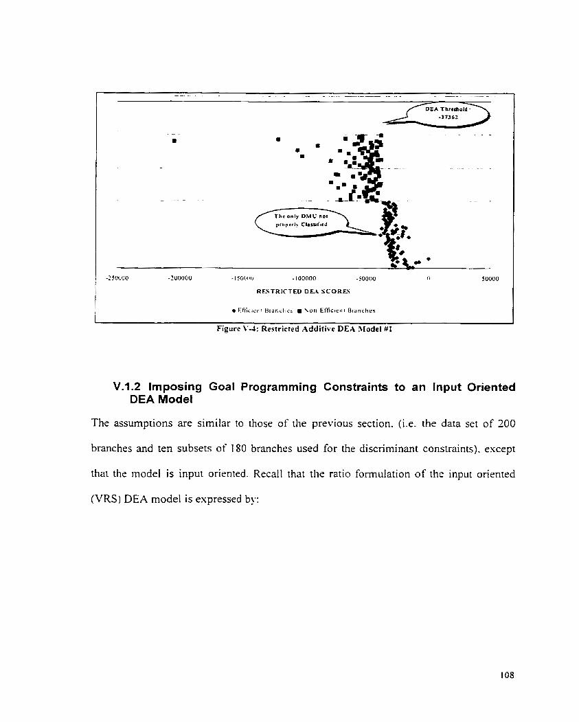
-200000 - 1 !G(~IIIJ - 100000 -C0000 0 50000

RESTRICTEU DE4 SCORW

1

Figure \'4: Restricted Additive DEA 3lodel # I

V.1.2 lmposing Goal Programming Constraints to an Input Oriented DEA Modef

The assumptions are similar to those of the prwious section. (Le. the data set of 200

branches and ten subsets of 180 branches used for the discriminant constraints). except

that the model is input oriented. Recall that the ratio formulation of the input oriented

(VRS) DEA model is espressed by:

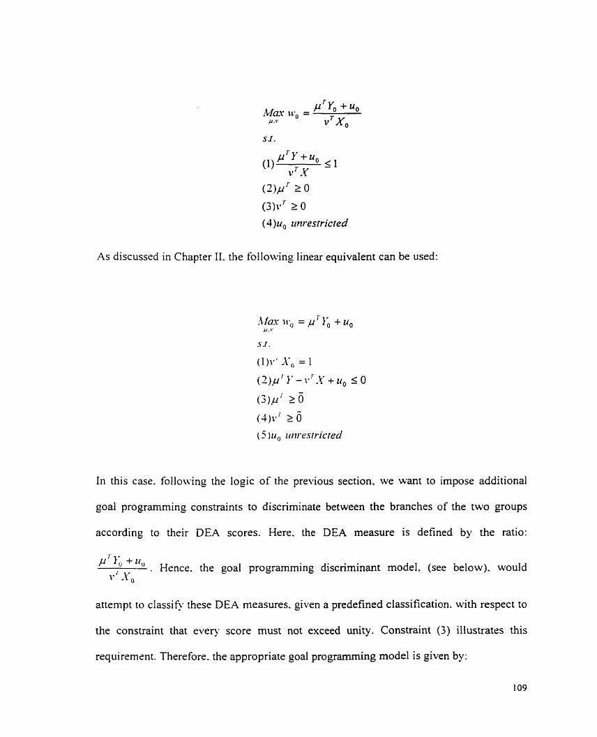
As discussed in Chapter II. the following linear equivalent can be used:

s . r .

( 1 ) r i xo = 1

( 2 ) p ' 1. - 1.' .Y + r r , 2 O -

( 3 ) p i 2 O

In this case. following the logic of the previous section, we want to impose additional

goal programrning constraints to discriminate between the branches of the two groups

according to their DEA scores. Here. the DEA measure is defined by the ratio:

,dl; + Zr" . Hsnce. the goal programming discriminant model, (see below). would

1- ' .Y,

attempt to classify these DEA measures. given a predefined classification. with respect to

the constraint that every score must not exceed unity. Constraint (3) illustrates this

requirement. Therefore. the appropriate goal programrning model is given by:

Let ;î, and 7 be the optimal values derived in this rnodel.

This formulation is clearly nonlinear. and in real situations. with large data sets. deriving

a solution can be computationally challenging. It can be important to avoid adding such

nonlinear restrictions into the input oriented model. The purpose of the esperiment herein

is to compare three approaches:

O The non-restricted input oriented model. expressed in its linear version:

O The input oriented model. with nonlinear goal programming constraints added. The

results computed by this enhanced DEA model take into account expert opinion,

expressed in a ratio forrn;

O The input oriented model. with linear goal programming constraints added. Indeed,

with this experiment. we wish to demonstrate that this c m be a good approximation

of the nonlinear version (Le. ratio constraints). The performance of this DEA model

will be compared with the two other cases. to determine if it can be used as a

replacement for the nonlinear version. and if it is providing bener results than a non-

restricted model.

V. 1.2.1 lmposing Nonlinear Goal Programming Constraints in an Input Oriented DEA Mode1

The nonlinear problem presented above was solved. and the optimal values derived were

inserted into the goal constraints, thereby transforming them into a linear form as follows

(this holds since the optimal values are now scalars):

Becausr M is a large scalar number, the constraints corresponding to the DMUs not

properlj- classified \vil1 aIways be verified. Therefore. the number of the constraints can

be reduced by the following formulation:

These constraints are then added to the linear form of the input oriented model:

This three-stage process. applied to the bank data set. is similar to the previous

esperiment. and Table V-2 summarizes the results of the ten restricted DEA rnodels

compared to the unrestricted DEA model. The last column dernonstrates that, on average.

the nonlinear restricted version of the DEA model is properly classifying 189.9 branches

out of 200 branches. I f we compare this average performance with the unrestricted

version. we recognize that it is doing better. both in terms of classification, and in terms

Table \'-2: Summarized Resufts For The Input Restricted Experiment

Figure V-5 plots the branch DEA scores for the unrestricted version. Again, we note the

same inconsistency with the bank consultants' classification. Indeed, sorne low

Thrcshold

o Of Properl) Classifird Branches = Of Non Properl? Classi ticd ,Branches

Unresrricted (0 )

Al

044481 030671 030851 02599

A2

03013 ( 1 )

A3

190' 1891 1901 188 I i l 7 ] . l g l

1

(4) 02449022361 03043

( 2 ) A4

le2i 191

( 3 5

29 j 9; 101 I l i 101 l l i 81 1 1 1 i I l ! 1 i 1 1

l I t / i l , ( ,

03342

A5

189

(6)

9

A6

02884,

12 I IB9 91

10 1 ,

I 1

191

0.3045 (7)

188

029318

A7 ( 8 ) A8

AI-Al0 (9) Average

(10) A9 AI0

performing branches are deemed efficient in a DEA sense (i.e. on the efficient frontier).

and some high performing branches have their benchmark being lower than some low

performing branches.

I O 1 O 4 0 6 O 8

SOS RESTRICTED D U S C O R S

Effic~cnt Branches . S o n Efficient Branches

Figure V-5: Non-Restricted Input DEA Model

Figure V-6 shows that the DEA scores are better classified for the nonlinear restricted

version than the non-restricted case. Also, there are no low perfoming branches on the

efficient frontier. This first experiment clearly means that adding nonlinear goal

programming constraints to the DEA mode1 can improve its accuracy. and more

importantly. its consistency with bank consultant expertise.

RESTRICTED D m SCORES

- - - - - - - O Efficicnr Branclics Son Efficient Brancliec

- . . - - - -

Figure V-6: Restricted Input DE.4 Xlodel #1 (Non Linear Constraints)

V. f.2.2 lmposing Linear Goal Programming Constraints in an Input Oriented DEA Mode!

This case assumes that the follo~ving linear goal prograrnming model can be used in place

of the nonlinear formulation. Notice that the constraint (3) indicates that every DEA score

must not exceed 1. In fact. even if kve used the net profit oriented form as an

approximation to the ratio fom. we still need to keep the original requirements of the

input oriented model. Hence. we have imposed the DEA constraints into the goal

programming model. to respect the nature of the DEA scores:

Ler 7, and 7 be the optimal values derived in this model.

In stage 2. the optimal values are replaced in the equations ( 3 ) and (4). so we can solve

the constrained DE.4 problem:

Again, this process is similar to the one used with the additive formulation. The final

stage cornputes the DEA model. and classifies the scores for each of the ten versions.

Table V-3 summarizes the results for the unrestricted version, and the ten restricted

models. The last column is the average of rhe ten restricted results. and gives an estimate

of the performance we can have with this approximation. We can see that 188.8 out of

200 branches are properly classified, while only 171 branches are properly classified with

the unrestricted version. This average performance is very close to the nonlinear

restricted performance (i.e. 189.9). Therefore, we can conclude that instead of using a

nonlinear form for restricting an input oriented model. one c m use its linear

approximation. and get close results.

Tabte V-3: Summarized Results For The Input Restricted Experiment (Linear Constraints)

Branchss ; Of Non Propcrl! Classificd Eranc hcs t Figure V-7 plots the DEA scores of the 200 branches when linear constraints are imposed

on the input oriented model. This graph is to be compared to the non-restricted graph

(Figure V-5). and to the restricted graph obtained with the nonlinear constraints (Figure

V-6). We can see that the discrimination of branches is quite similar to the one obtained

with the noniinear version. In addition. it is consistent with bank management

classification. with no low performing branch being efficient. and vice-versa.

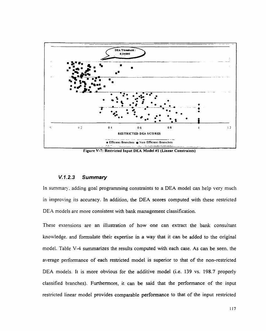
RESTRlCTEû DEA SCORES

Figure V-7: Restricted Input DEA Model#l (Linear Constraints)

V.1.2.3 Summary

In summary. adding goal programming constraints to a DEA model can help ver). much

in iniproving its accuracy. In addition, the DEA scores computed with these restricted

DEA models are more consistent with bank management classification.

These extensions are an illustration of how one can extract the bank consultant

knowledge. and formulate their expertise in a way that it can be added to the original

model. Table V-4 summarizes the results computed with each case. As can be seen. the

average performance of each restricted model is superior to that of the non-restricted

DEA models. It is more obvious for the additive model (Le. 139 vs. 198.7 properly

classified branches). Furthermore, it can be said that the performance of the input

restricted linear model provides comparable performance to that of the input restricted

nonlinear version.

Table V J : Summary Of Restricted DEA Model

Non-Restricted DEA Model (k of properly classified

branches out o f 200)

Average Performance o f Resûicted DEA Mode1

(# o f properly ciassified branches

Additive Oriented Model

1 linear version) I l L

Input Oriented Model (non

139

approximation)

. .

out o f 200) 198.7

l

Input Oriented Model (linear

.A second type of improvement is the way DEA models compute the branch scores.

Indeed. with non-restricted models. somr inconsistency can appear such as having low

performing branches being efficient in ternis of DEA measure. With restricted models.

the DEA scores become more consistent with branch consultants' perceptions, and there

would appear to be less likelihood of low performing branches being deemed efficient. in

terms of DEA benchmarking.

171 189.9

171 188.8

V.2 EXTENSION TO MORE THAN TWO CLASSES

We have demonstrated. thus far. how to handle branch consultant expertise, and more

specificall y classrficorion infornlarion of branches within two groups: high and low

performing branches. In many cases we will have to deal with more sophisticated

classifications. involving more than two groups, for example, High. Medium. and Low

performing branches. The approach that c m be used in such instances would be similar to

the methodology developed previously. with the oniy difference being that the goal

prograrnming discriminant mode1 has to be adapted to that kind of situation (Figure V-8).

No esperiment n i I l be performed in this case. Rather, we describe the methodology. and

the different models that can be appIied in such situations.

FTETOT SlDPSCTRF

PF4 \f&

Figure V-8: lmposing Goal Programming Constraints On A DEA hlodel (3 Croups)

The basic problem to be addressed initially may be brieflp described as follows. Group

membership for a set of p-dimensional points is knoun. A simple weighting scheme is

sought to 'score' each p-dimensional point by weighting its components. The scores will

be divided into intervals designed to ensure. where possible. proper grcup assignment. By

extension, the scoring (weighting) scheme rnay then be applied to addirional points in the

space in order to determine likely group membership. This provides insight into the

relative importance of dimensions in segregating groups.

The problem can be stated as follows [95GF]: Given points A, and sets G,. find the linear

transformation X. and the appropriate boundaries (interval subdivisions) b: and b l , to

properly categorize each A, (Bounds b: and by represent respecti\dy the loufer and

upper boundaries for points assigned to group j). Thus. the task is to determine a linear

predictor or weightinf scherns X. and breakpoints b! and by . such that:

The boundary constraints in (2) designate a specific ordering of discriminant scores,

requiring, for example. that Group 1 scores be generally lower than Group 2 scores,

Group 2 scores be generally lower than Group 3 scores. and so on. This particular

sequencing may prove too restrictive to produce the most effective discriminant solution.

An alternative formulation may be considered. This formulation would impose boundary

separalion as a common constraint. seaing as a goal. the inclusion of points within

appropriate bounds:

Min a,

(3)b: <b:+, for j = 1.-.-.g-1

where g = nurnber of designared grozrps

We finally obtain a more refined formulation by introducing d, which is the distance of

points A, from its adjusted boundary. Therefore. we can effectively combine the goal of

minimizing boundar!. deviations with that of maxirnizing the surn of these distances:

S.I .

1 ) d , = b a , j o r d U , E G ,

(7).+k'+d,=b)+a, f o i - u l l A , ~ G ,

(3)by 5 b:+, for j = 1.-.-.g - 1

iiqhere g = number of designured groups

If the brancli consultants had provided a branch classification composed of three groups

(Low. Medium and High performing branches), we would use the following approach:

Stage 1: Use the multigroup goal programming mode1 presented above, applied to

our three group case (let G1 be the group of low. G3 the group of medium and G3 the

group of high performing branches). The signs of the goal programming coefficients

will determine the inputs and outputs for subsequent DEA analyses (i.e. additive.

input.. .).

Stage 2: Restrict the multipliers such that the three groups of branches in the analysis

sarnple (say 180 branches) are separated to the greatest extent possible. Notice that.

depending on the DEA model we want to work with. we impose additional

constraints in the goal programming discriminant rnodel to respect the DEA model

requirements. If we choose to work with an additive model, the following goal

programrning discriminant formulation will try to discriminate the additive DEA

scores :

for d l A, E G , for a// A, E G,

In the case of an inpur model. solve the linear approsimation of the multigroup goal

programrning constraint model. with additional constraints that take into account the

input DE.4 mode1 requirements:

S.!.

( I ) P ~ Y -V 'X + u, -d , = bj -a, fornllA, E G ,

( 2 ) p T ~ -Y ' .X t u , + d , = b: +a, for alZ A, E G , (3)by s hJ-, jor j = 1.---.g - l

(4),uTy + z r , S n' X

(5)/YT 2 O

(6)vT 2 O

( 7 ) rc , rtnrestricred

where g = nrimber of designated grorrps

Stage 3: Let d l , 6:-, by . â, be the optimal values derived in either of these two

models. These optimal values are then replaced in the corresponding modified DEA

models (Le. additive. input.. .). and the branches are classified according to their DEA

scores. The DEA scores will be improved. and more in line with what branch

consultants are expecting. The nest formulation will be used if we decide to apply the

additive oriented model:

( 3 ) ~ ' y - v' X + t r , + d , = by +a, foraZlA, E G ,

( 4 ) p T 2 1 -

(5)v7 2 1

(6)u, unr-estricted

With an input oriented model instead. the following formulation will be used:

V.3 SENSlTlVlTY ANALYSE

The previous experiments were based on additive and input DEA models using data sets

of fixed size: 200 branches with 180 classified as good and poor performing by the

branch experts.

The pr imas objective of these experiments was not to test the predictive capabilities of

such models. but rather to compare improved DEA models (by determining inputs and

outputs or by imposing additional constraints), with other DEA models built randornly.

In this case. ~vhile branch consultants classified 180 branches out of 200. it would be

interesting to know how the various analysis sample sizes work. if one were now

approaching a new Bank uith the idea of building such an "Expert DEA" model for them.

Since there c m be significant effort needed on the part of branch consultants to arrive at

a reliable classification of branches. it would be ver). useful to h o u - that an analysis

sample size of sa!. 10 is nor adequate. but that a size 40 can classify significant branches

out of the 20 holdouts, and that more than 40 analysis branches, gives us very little

improvement. To know that we c m rely on the results from an anaiysis of 30 or 40

classified branches. as opposed to 200 can have a major impact on the usefulness of the

DEA tool. In addition. the less qualitative information imposed by the expert. the more

objective will be the analysis.

To test this hypothesis. the entire exercise had been carried out with smaller analysis sets

(1 0, 20, 40, 60. 100. 180). with a remaining set of 20 branches being kept as a holdout

sarnple, and inserted into the final model in the predictive stage. Table V-5 displays the

results from the input experiment. The results show how the hold out samples of 20 are

classified in these instances. versus the way they ended up in the models that used an

analysis sarnple size of 180 DMUs.

The first cohmn indicates the number of branches used dunng the analysis stage, to build

the DEA models. Thsss branches have been classified by the consultants, and the

experiment was run. starting from 10 to 180 classified branches. The second colurnn

indicates for each case. the number of DMUs out of the 20 hoIdout units that were

properly classified. This number is an increasing function of the analysis sample size. as

u-ouId be espected. The last column indicates the percentage of branches properly

classified.

Table \'-5 : Sensitivity Analysis W i t h Iriput DEA Models Csing Samples Of Different Sizes

In summary- we can sas that a small analysis sarnple (say 40 DMUs). can yield good

results in ternis of classification. Therefore, one couid apply our rnethodology, with a

relatively small number of classified branches. Hence. a reIatively small amount of

qualitative information is required from the organization in order to gain significant

irnprovements in the DEA performance model.

# DMUs in Analysis Set

1 O 20 40 60

1 O0 180

# Holdout Branches (out of 20) Properly Classified

13.4 14.2 14.9 15.7 16.2 16.9

% Holdout ProperIy Classified 62% 71% 75% 790/0 81% 85%

VI. CONCLUSIONS

This thesis has demonstrated hou. DEA, when improved. can be a powerful

benchmarking technique. and a managerial tool that can help bank management apply

strategies to improve their branch network efficiency. Enhanced DEA models have been

presented. to take into account. not only standard information. but also other types of

information such as expertise. These DEA models. obtained using Our approaches. have

two main advantages:

The? compute more refined scores. and outperform most of the other DEA models

that might have been defined differently (by selecting variables arbitrarilp or

randomly). For instance. an additive model with inputs and outputs defined using

expert knowledge and discriminant techniques. out performs 93% of the set of DEA

models. with variables randomly defined. In addition. an additive model with

additional goal programming constraints. representing branch consultants

classification. is better than a non-restricted mode1 (1 98.7 properly classified branches

out of 200 vs. 139).

The branch consultants are more likely to accept the computed measures. and use

them as managerial tools. Indeed. these improved DEA models compute efficiency

scores for each branch that are more consisrent with branch experts' perceptions.

These rnodels will help managers benchmark branches' and eventually apply

strategies (by reducing inputs or increasing outputs) to bring inefficient branches onro

the efficient frontier.

We have created a methodology that combines standard performance measurement tools

(DEA) and discriminant techniques. and have demonstrated that the DEA model being

applied. can be improved in many ways:

Selecting inputs and ourpzits ivith the help of discriminant techniques. Goal

programming appears to be the best tool. if we decide to work with an additive

model. If the selected model is input oriented. logistic regression is slightly better

than goal programming.

Rrs fricr iitg the goal progranming nt ulripliers. when experts have un opiniort abolrr

[hr orientarion of sonle ini-iables. This has the effect of reducing the number of

possible combinations. and helps in defining inputs and outputs for the remaining

variables. The resuits are very good for both additive and input models.

Iïltposiitg additional consrrainrs i~ the DEA nzodel to reflect the bl-anch classification

giiqen b~n the experr. This feature not only improves the performance of the models.

bur also their way of benchrnarking the units. Indeed, the obtained scores are more

consistent with what the expert perceives. using their own knowledge and classical

techniques.

In this thesis we demonstrated how one can extract expert knowledge and formulate it to

irnprove DEA models in many different ways. This idea can clearly be extended to a

DEA expert system that could not only be improved once, but could learn from additional

expertise. and from itself. It could be a learning process by way of incremental

knowledge (Figure VI-1). The DEA model would use standard data on Say 200 bank

branches (1). and classification knowledge (2), on, Say. 60 branches (3), whose

performance we know. This improved DEA model would benchmark the units (4), so

that the managers c m apply strategies to bring the inefficient branches ont0 the frontier.

The experts will l e m from the DEA mode1 to increase hisher knowledge about the

branch network (5). This additional knowledge would be mixed with field observations

(6). to become a part of rheir expertise. and to increase the information used by the Model

- 20 DMUs

20 DMUs

classi tled (Heuristics)

Standard Data Performance (200 DMUs)

Irnproved DEA Model (DEA scores)

Follow-up branch Network

performance Figure VI-1: DEA Learning Model

These experiments couid be carried out on other data sets which would provide more

results that could confirm our methodology, and the improvements obtained with such

DEA models.

The approach that could be adopted in real cases would be the following:

1. An initial screening process would be applied to help identify the most significant

variables (using a statistical tool such as factor analysis) and to define the flexible

variables. the prcdcfined inputs and outputs. and the variables to retain because the

branch consultants want to apply strategies on them (reducing inputs or improving

outputs):

2. An analysis stage. using a small data set (40 DMUs can be sufficient), would then be

applied to determine the inputs and outputs among the flexible variables;

3. A bencharking stage would then follow. that cornputes DEA scores for the

branches. using the DE.4 mode1 defined in the previous stage. The branch consultant

should be receptive to the identified benchmark branches. as these would be

consistent with his own knolvledge. This being the case. one would anticipate that

strategies ~ o u l d be applied to bring inefficient branches on the efficient frontier;

4. A final predictivc stage could then be employed to integrate new branches. This

would aid in setting performance targets for those branches.

VII. APPENDIX

Vil.? FACTOR ANALYSIS

VII.1 .l Introduction

The general purpose of factor analysis is to find a way of condensing (summarizing) the

information contained in a number of original variables. into a smaller set of new

composite dimensions (factors), with a minimum loss of information.

Factor analysis attempts to identie underlying variabIes. or factors. that explain the

pattern of correlations nithin a set of observed variables. Factor analysis is often used in

data reduction. by identifiping a small number of factors which explain most of the

variance observeci in a much larger number of manifest variables. Factor analysis can also

be used to generate hypotheses regarding causal mechanisms. or to screen variables for

subsequent analysis (for example- to identify collinearity prior to a linear regression

anaIysis).

Variables that are correlated with one another. but largely independent of other subsets of

variables. are combined into factors.

The GLM General Factonal procedure, provides regression analysis and analysis of

variance for one dependent variable by one or more factors andor variables. The factor

variables divide the population into groups. Using this general linear mode1 procedure.

we can test nul1 hypotheses about the effect of other variables on the mean of various

groupings of a singIe dependent variable.

Factor Analysis is particularly suitable for analyzing cornplex. multidimensional

problems. This technique c m be utilized to examine the underlying patterns or

relationships for a large number of variables, and to determine whether or not the

information can be condensed or summarized into a smaller set of factors or components.

Factor Analysis. (unlike multiple regression. discriminant analysis, or logistic regression.

in which one or more variables are explicitiy considered the cnterion or dependent

variable. and ali others the predictor or independent variables), is an interdependence

technique in which a11 variables are simultaneously considered. In fact, each of the

observed (original) variables is considered as a dependent variable that is a function of

some underlying. latent. and hypothetical set of factors (dimensions).

Factor Analysis can perform four functions:

1. Identify a set of dimensions that are latent in a large set of variables; this is referred to

as R factor analysis.

2. Devise a method of combining or condensing large numbers of people into distinctly

different groups within a larger population; this is referred to as Q factor analysis.

3. Identify appropriate variables for subsequent regression, logistic, or discriminant

analysis from a much larger set of variables.

4. Create an entirely new set of a smaller number of variables to partially or completely

replace the original set of variables for subsequent analysis.

Factor analysis c m achieve each of the purposes from either an exploratory (useful in

searching for structure among a set of variables or as a data reduction method). or

confirmatory perspective (assess the degree to which the data meet the expected structure

of the analyst).

V11.1.2Factor analysis vs Component analysis

Numerous variations of the general factor model are available. The rwo most frequently

employed factor analytic approaches. are component analysis (or principal components

analysis) and common factor analysis. Selection of the factor model depends on the

objectives. The component model is used when the objective is to summarize mosr of the

original information (variance) in a minimum number of factors for prediction purposes.

In contrat, the common factor analysis is used primarily to identiQ underlying factors or

dimensions not easily recognized (only shared variance is analyzed).

V11.1.3 Factor Analysis Decision Diagram

The next figure shows the general steps followed in any application of factor analysis. If

the objective is data reduction and summarization, factor analysis is the appropriate

technique to use. The sample size should be 100 or larger. As a general mie. there

shouId be four or five times as many observations as there are variables to be analyzed.

In the second step, the alternative would be to examine either the correlations between

the variables, or the correlations between the observations. if the objective is to

sumrnarize the characteristics, the factor analysis would be applied to a correlation matrix

of the variables (R Factor Analysis). If the objective is to summarize the observations.

the factor analysis would be applied to a correlation matrix of the observations (Q Factor

Analysis). The Q Factor PLnaIysis approach is not utilized very frequently because of

computational difficulties. Cluster analysis or hierarchical grouping. are more designed

for this approach.

In the third' step. we need to specify how the factors are to be extracted: orthogonal

factors (each factor is independent from al1 other factors). or oblique factors (the

extracted factors are correlated). Orthogonal solutions are mathematically simpler to

handle. while oblique factor solutions are more flexible and realistic. If the goal is to

reduce the number of original variables. regardless of how meaningful the resulting

factors may be. the appropriate solution would be an orthogonal one. Also. if we want to

reduce a Iarger number of variables to a smaller set of uncorrelated variables for

subsequent use in a regession or other prediction technique. an orthogonal solution is the

bsst. If the goal is to obtain several theoreticaIly meaningful factors or constructs. an

oblique solution is more appropriate.

In the next step. \Te examine the Unrotated Factor Matrix to explore the data reduction

possibilities for a set of variables and obtain a preliminary estimate of the number of

factors to extract.

In the following stsp. the factor matris is rotated to obtain the final number of factors and

their interpretation.

Then, we may stop there or proceed with subsequent analysis using other techniques such

as Logistic Regression. Discriminant Analysis, or even Goal Prograrnming. For this

purpose, we would esamine the factor matrix and select the variable with the highest

factor loading as a surrogate representative for a particular factor dimension.

If the objective is to create an entirely new set of a smaller number of variables,

composite factor scores would then be used as the raw data to represent the independent

variables in a logistic, or discriminant analysis.

I l FACTOR MODEL

Factor Analysis or Cornponenf &~alysis

Orthogonal or Oblique

UNROTATED FACTOR hL4TRIS

Number of factors.

-

ROTATED FACTOR MATRI S I Il Factor in~erpretation. I

--L6JS FACTOR SCORES I

I For subscquent analysis (Log. Reg. MDA) -

Sequence of Analysis

Vll.l.4The rotation of Factors

The reference axes of the factors are tumed about the origin until some other position has

been reached. The simplest case is in an orthogonal rotation in which the axes are

maintained at 90 degrees.

Rotation of the factors. in rnost cases, improves the interpretation by reducing some of

the ambiguities that often accompany initial unrotated factor solutions. Generdly,

rotation will be desirable because it simplifies the factor structure. and because it is

usually difficult to determine whether unrotated factors will be meaningful or not.

Unrotated factor solutions extract factors in the order of their importance (the first factor

accounts for the largest amount of variance).

The oblique solution provides us with information about the extent to which the factors

are actually correlated with one another.

When the objecti1.e is to utilize the factor results in a subsequent statistical analysis, we

should always select an orthogonal rotation procedure. because the factors are orthogonal

and thrrefore elinlinate coliinearity. However, if we are simply interested in obtaining

theoretically meaningful constructs or dimensions. the obtique factor rotation is more

desirable. because it is theoretically and empirically more realistic.

In a factor matrix. columns represents factors, with each row corresponds to a variable's

Ioading on a factor. Three major orthogonal approaches have been developed:

QUARTIMAX Rotation: the goal is to simplify the rows of a factor matrix (i.e.

masimizing a variable's loading on a single factor).

VARIMAX Rotation: the goal is to simplifi the columns of the factor matrix (Le.

making the number of "high" loadings as few as possibIe). This approach seems to

give a clearer separation of the factors.

EQUIMAX Rotation: it is a compromise between the QUARTIMAX and the

VAFUMAX criteria.

The following graph shows the five variables plotted in the two selected component

spaces. after their rotation (using SPSS Software).

Component Plot in Rotated Space

Component 1

VIL1 .SCriteria for the Nurnber of Factors to Be Extracted

An esact quantitative basis for deciding the number of factors to extract has not been

developed. Latent Root' A Priori. Percentage of Variarice and Scree Test criteria. are the

techniques for the number of factors to extract, currently being utilized.

Vli. 1.5.1 Latent Roo t Criterion

In Component Analysis, in which 1's are inserted in the diagonal of the correlation

matrix. and the entire variance is considered in the analysis. only the factors having latent

roots (eigenvalues) greater than 1 are considered significant: al1 factors with latent roots

less than 1 are considered insignificant and disregarded. On the other hand. with

Common Factor Analysis. the latent root criterion should be adjusted slightly downward;

the eigenvalue cutoff level should be lower. and approximate either the estimate for the

common variance of the set of variables or the average of the communality estimates for

al1 the variables. In many cases. any positive eigenvalue obtained in a Common Factor

Analysis \vil1 qualify the corresponding factor.

V11. '1.5.2 A Priori Criterion

With the a priori criterion. kve already know how many factors are to be extracted. The

cornputer will stop the anal>-sis when the desired number of factors has been extracted.

VI/. 1.5.3 Percen tage of Variance Criterion

The cumulative percentages of the variance extracted by successit:e factors are the

criteria. In many cases. the factoring procedure should not be stopped until the estracted

factors account for at least 95 percent of the variance or until the last factor accounts for

only a srnall portion (less than 5 percent). Where information is less precise. we can

consider a solution that accounts for 60 percent (or even less) of the total variance as a

satisfactory solution.

VI!. 1.5.4 Scree Test Criterion

The scree tail test is an approach used to identify the optimum number of factors that can

be extracted. before the arnount of unique variance begins to dorninate the cornmon

variance structure. This test is derived by plotting the latent roots against the number of

factors in their order of extraction. and the shape of the resulting curve is used to evaluate

the cutoff point.

The following graph shows the scree plot for Our data set. Using the eigenvalue of 1 as a

cutoff. the first two components (factors) will be extracted. In general. the scree test will

result in at least one, and sometimes two or three more factors being considered as

significant than \vil1 the latent root criterion.

Scree Plot

i

1 2 4

Component Nurnber

Total Variance Explainad

VII.l .GCriteria for the significance of Factor Loadings

Extraction Meihod Principal Componenl Analysis

Camooneni 1

2 3 4

5

Roiaiion Sums of Squared Loadinqs Extraciion Sums of Squarw Loadinqs Cumulative

Ok 49.587' 77.341

Total 2.479 1 388

ln~iial Eiqenvalues K cf

Variance 49.587 27 755

Cumulaiive % 49.722 77.341

Toiai 2.486 1.381

Toial 2 486 1 381 ,636 375 122

% of Variance

49.722 27,620

% of Variance

Cumulaiive U

49.722 i 49.722 27 620 12.715 7.508 2.436

77.341 90.057 97.564

1OOOOO

In interpreting factors, we must decide which factor loadings are worth considering.

Different approaches can be applied, such as:

Defining a scale describing the importance of factor loadings (.50 and more are very

important factor loadings, .40 are important and .30 are considered significant).

Another way would be to use a similar approach to that of interpreting correlation

coefficients. If the sample size is 100 or less? loadings of at least .19 and -26 are

recommended for the 5 and 1 percent IeveIs, respectiveIy. When the sampIe size is

200. .14 and .18 are recornmended for the 5 and 1 percent levels significance. When

the sample size is 300 or more, . I l and .15 are recornmended for the 5 and 1 percent

levels

As the number of \*aiables being analyzed increases. the acceptable IeveI for considering

a loading significant. decreases. Adjustment for the number of variables is increasingly

important as one moves from the first factor extracted to later factors. The larger the

sarnple size. the smaller the loading to be considered significant. The larger the nwnber

of variables being analyzed, the smaller the Ioading to be considered significant. The

larger the number of factors, the larger the size of the loading on later factors to be

considered significant for interpretation.

VI1.1.7 Limitations

One of the problems with Principal Component Analysis and Factor Analysis is that there

is no criterion beyond interpretability such as group membership. against which to test

the solution.

A second problem with these techniques is that, after extraction, there are an infinite

number of rotations available. al1 accounting for the same amount of variance in the

original data but with factors defined slightly differently.

Factor Analysis is frequently used in an attempt to "save" poorly conceived research.

V11.1.8 Matrix Formulation of the Factor Analysis Model

Principal Component Analysis and Factor Analysis produce a set of matrices depending

on the technique and the options chosen during the stages:

Observed Correlation Matris : Correlation matrix produced by the observed variables.

Reproduced Correiation Matris : Correlation matrix produced from factors.

Residual Correlation Matris : Difference between Observed and Reproduced

Correlation matrices. A small Residual Correlation Matrix indicates a close fit

between Observed and Reproduced Correlation matrices.

Factor-Score Coefficients Matris: Matrix of coefficients used to estirnate scores on

factors from scores on observed variables for each individual.

If rotation is orthogonal (factors are uncorrelated), a loading matrix is produced

which is a matrix of correlations between observed variables and factors.

If rotation is obrique (factors are correlated), the Factor Correlation Matrix contains

the correlations among the factors. The loading matrix splits into two matrices: a

structure rnatrix of correlations between factors and variables and a pattern matrix of

unique relationships between each factor and each observed variable.

1; Imatrix iandob1i4ue Variable matrix Both orthogonal

and obli ue Factor-score Both orthogonal

La bel R

Name Correlation

A

Rotation Both orthogonal'-

matrix 1 and oblique Factor loading 1 Orthogonal matrix Pattern matrix

Oblique

I

B

C

Eigenvalue Both orthogonal 1 1 matrix and obliaue

0

uenvector Both orthogonal and obliaue

Factor-score coefficients matrix Structure rnatrix

p : number of v a i a b l e s . ~ : number of su

Both orthogonal and oblique

ObIique I

Factor correlation matrix

1

N x p 1 Matrix of standardized observed variable

Size p x p

Oblique

Description Matrix of correlations between variables

N x m

1 estirnate theunique contribution of each [

scores Matrix of standard scores on factors or

p x m

factor to the variance in a variable. If orthogonal, also correlations between

components Matrix of regression-like weights used to

1 variables and factors. p s m 1 Matrix of regression weights used to

cenerate factor scores from variables I - I

p s m ( Matrix of correlations between variables

m s m Diagonal matris of eigenvalues. one per I factor

m s m

p S rn ~ a t r i s o f eigenvoctors. one vector prr I ei~envalue. I

and (correlated) factors Matris of correlations among factors

--

~jects. m : number of factors or components

V11.1.9Factor Analysis Key Terms

Common Factor Analysis: A factor mode1 in which the factors are based upon a

reduced correlation matrix. That is. commonalties are inserted in the diagonal of the

correlation matrix, and the extracted factors are based only on the common variance. with

specific and error variance excluded.

Communality: The amount of variance an original variable shares with al1 other

variables included in the analysis.

Factor: A linear combination of the original variables.

Factor loadings: The correlation between the original variables and the factors, and the

key to understanding the nature of a particular factor. Squared factor loadings indicate

what percentage of the variance in an original variable is explained by a factor.

Factor matrix: A table displaying the factor loadings of al1 variables on each factor.

Factor rotation: The process of manipulating or adjusting the factor axes to achieve a

simpler and pragmatically more meaninghl factor solution.

Factor score: Factor analysis reduces the original set of variables to a new smaller set of

variables. or factors. U'hen rhis new smaller set of variables (factors) is used in

subsequent analysis (e.g.. Logistic Regression), some measure or score must be included

to represent the newly derived variables. This measure (score) is a composite of al1 of the

original variables that n-ere important in making the new factor. The composite measure

is referred to as a factor score.

Oblique factor solutions: A factor solution computed so that the extracted factors are

correlated. Rather than arbitrarily constraining the factor solution so the factors are

independent of each other. the analysis is conducted to express the relationship between

the factors that ma. or ma) not be orthogonal.

Orthogonal factor solutions: A factor solution in which the factors are extracted so that

the factor axes are maintained at 90 degrees. Thus each factor is independent of. or

orthogonal from. al1 other factors. The correlation between factors is arbitrarily

determined to be zero.

VIL2 DATA SET PROVIDED BY THE BANK

Branch r

98 99

100

IO1

102

IO3 39.65 125 582 6555 952 4933 1

MOPCAO

1 872

4785

820

442 1 31 18

FTOT

317

9.61 411

13 79

9.17

MDPMTRF

217

57 1 90 77 1 187

RSP

6

70

5 30

17

LOANTOT

131 346

165

189 129

MWDMWPD

1329 3891 407 3532 1868

Dummy Variable

1 I 1 1

i

Observed

O O O

1

1

Branch #

148 149 150 151 152 153

FTOT

11.73 14.78 10.38 5.72

18.71 12.12

RSP

10 22 18 6

33 29

LOASTOT

166

22 4 149 126 709 1 93

hlOPC.40

3054

MDPMTRF

436 4239 4012 3092 3950

4408

Obsrrvrd

1

MWDMWPD

ZOO0 458 407 296 657 596

1 1

I 1 1

Durnmy Variable

I 1879 7854 3152 3 33-1

3 533

1

1 1

I 1

Observed

1 1

1

BranchX

198 199 200

FTOT

1982 26.75 4 1 7

LOANTOT

179 332 2-1

MDPMTRF

264 340

RSP

31 47

1

hlOPC.40

3391 3 825

42

MWDMWPD

2625 3100

Durnrny Variable

1 1

3001 23 1

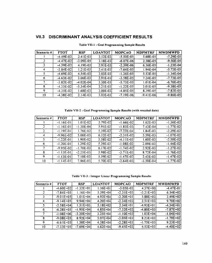
V11.3 DISCRIMINANT ANALYSE COEFFICIENT RESULTS

Table VIL1 : Goal Programming Sample Results

Scenario # 1 FTOT 1 RSP

Table VIL2 : Goal Programrning Sample Results (with rescaled data)

Table 1'11-3 : lnteger Lincar Programrning Sample Results

Scenario # FTOT RSP 1 -4.60E102 -1.32E-0 1

MWDMWPD - 1.36E-02

LOANTOT MOPCAO MDPMTRF MWDMWPD 1.36E+O 1 -3 .O5 E-02 4.37E+00 -4.47E-0 1

Scenario #

1 LOANTOT 1 MOPCAO

5.79~-021 - 1.66E-02 FTOT -1.16E-O 1

MDPMTRF 1.62E-03

RSP 1 .O 1 E-02

Table VI14 : Integer Linear Programming Sample Results (with rescaled data)

Scenario f: 1 7 - 3 4 5 6 7 8 9 1 O

Table VI14 : Multiple Discriminant Analyis Sample Resutts

MDPMTRF -2.27E-02 4.38E+00 -8.90E-03 -3.47E-03 - 1.45E-02

-4-07E+00 -6.23 E+O 1 -5.84E-03 -6 .HE-02 -7.9 1 E+00

Scenario # FTOT RSP 1 -5.92E-01 7.85E-03

MWDMWPD -9.40E-03 -2.24E+00 -3.75E-03 - 1 26E-03 5.68E-03

-2.32Ei-00 4.58E+0 1 -6.16E-03 3.9OE-02

LOANTOT MOPCAO MDPMTRF MWDMWPD 5.8 1 E-03 1.9 1 E-04 -3.20E-04 -4.88E-04 5.82E-03 2.3OE-04 -4.34E-04 -4.70E-O4

FTOT -3.6OE-O l -3.47E102 -2.48E-0 1 -2.32E-0 1 -2. I3E-0 1 -2.32E-07 -6.9 1 E-02 -2.23E-O 1 -6.2 1 E-O 1

RSP 2.95E-02 1 -5 1 E+O 1 1.65E-02 1.3 1E-02 8.94E-03 l.36E+01 5.69E+O 1 I.32E-02 7.84E-02

LOANTOT ].OIE-O1

4.6 1 E+O 1 5.60E-02 4.39E-02 8.3 1 E-02

4.36E+OI 2.06E+-02 4.9 1 E-02 1.89E-0 1

4.13E+OI -1.82E702i 1.40E+Oi

MOPCAO -3.1 0E-02

-9.22E+00 - I .3 1 E-02 -8.14E-03 4.08E-02

-6.64E-iOO -1 -2 1 €+O2 -8.79E-03 -1.01E-01

-3.lJE+00

VIII. REFERENCES

Agrell P. J.. Steuer R. E. ( 1997). Faculty Performance Evaluation Using Data Envelopment AnaZyszs. Working Paper WP-246, Department of Production Econornics. Linkoping Institute of Technology.

Ali A. 1.. Lerne C. S.. Seiford L. M. (1995). Components Of EfBciency Evalzrat ion In Data Enveiopment Analysis Models. European Journal of Operational Research 80(3), 462-473.

Ali A. 1,. Seiford L. M. (1990). Translation Invariance In Data Eni.elopntettt Ana!l.vsis. Operations Research Letters 9(5), 403-405.

Banker R. D. ( 1 984). Estimating AMosr Productive Scale Siie Using Data Emelopntent 4nah.si.s. European Journal of Operational Research 17. 3 5-44.

Banlier R. D.. Charnes A.. Cooper W. W. (1984). Some Models For The Estit?tation Of Technical And ScaZe Inefjiciencies In Data EnveZopnent -4naiysis. Management Science 30. 1078- 1092.

Banker R. D.. Charnes A.. Cooper W. W.. Swarts J., Thomas D. (1989). An hfr-odzrctiort To Data Envehpment Analysis With Some Models And Tlieir L'tes. Research in Government And Non-Profit Accounting 5. 125-164.

Barker K.. Szpakowicz S. ( 1995). Interactive Semantic AnaZ'sis Of Clazrse-Leiyel Relationships. Proceedings of the Second Conference of the Pacific Association for Computational Linguistics. Brisbane. Australia.

Becker S.. Selman B. ( 1986). An Overview Of Knowledge Acquisition Methods For Expert Systems. Tech. Rept. CSRI, University of Toronto. Computer Systems Research Institute.

Bogeto fi P. (1 994). Incentive Ef$cient Production Frontiers: An Agencj? Perspective On DEA. Management Science 40,959-968.

Bogetofi P. (1 996). DEA On A Relaxed Cunvexity Assumption. Management Science 42(3), 457-465.

[93 CP]

Boose J.H. (1986). Expertise Transfer For Expert Sysiem Design. Amsterdam Elsevier.

Boose J.H. ( 1 986). Personal Consrruct Theory And The Transfer Of firman Expertise. Proceeding of the fourth National Conference on Artificial Intelligence. Austin, TX. 27-33.

C harnes A.. Cooper W. W. ( 1 962). Prograrnming With Fractional Fzinctionuls. Naval Research Logistics Quarterly 9,67-88

Charnes A.. Cooper W. W., Golany B., Seiford L. M., Shutz J. (1995). Forlndarions Of Data Envelopment Analysis For Pareto-Koopmans Efficien~ Enzpirical Producrion Funcrions. Journal of Econometrics 30. 91-107.

Charnes A.. Cooper W. W., Golany B., Seiford L. M., Stutz J. (1983). Invariut~t kftdriplicative Efflciency and Piecewise Cobb-Dotiglas Envelopments. Operations Research Letters 2(3), 10 1 - 1 03.

Chames A.. Cooper W. W., Lewin A. Y ., Seiford L. M. (1 993). Daru Emclopnzenr .-l nul~sis: Theory. Methodologt: And Appl icarions. Kluwer Academic Publishers. Boston.

Charnes A.. Cooper W. W.. Rhodes E. (1 978). hleasziring The Efficiency Of Decixion A4aking Units. European Journal of Operations Research 2. 429-344.

Charnes A.. Cooper W. W., Rousseau J. J., Semple J. H. (1 987). Daru Enivloptmnt A nalysis and Axiornatic Notions Of Efficiency And Reference Sets. Research Paper CCS 558, Center for Cybemetic Studies. University of Texas, Austin.

Charnes A.. Cooper W. W., Wei Q. L.. Huang C. H. (1987). Cone Ratio Data Eni-elopment A nalysis and Multi-Objective Programming. CCS Research Report no. 559, Center for Cybernetic Studies, University of Texas. Austin

Clark P., Matwin S. (1993). Learning Decision Theories From Absrracr Backgomd Kno~dedge. Proceedings of the European Conference on Machine Learning. Vienna, Austria, 360-365.

Clark P., Matwin S. (1993). Using Qualitative Models To Guide Indzrcrive Lenrning. loth ~nternational Conference on Machine Learning. Amherst, MA, 49-56.

[9 1 WC]

[O 1 WC]

[93 WC]

[96 WC]

[94FR]

[96FR]

[96FRP]

[57FM]

[8 1 GF]

Cook W. D.. Ali A. 1.. Seiford L. M. (1991). Strict Vs. Weak Ordinal Relations For Mrtltipliers In Dam Envelopment Analysis. Management Science 37 (6). 733-738.

Cook W. D.. Hababou M. (200 1). Sales Performance Meusuremenr In Bank Branches. Omega, The International Journal Of Management Science 29.299-307.

Cook W. D.. Kress M.. Seiford L. M. (1993). On The Use Of Ordinal Data In Dara Eni*elopment Analysis. The Journal Of The Operational Research Society 44(2). 1 33- 140.

Cook W. D.. Kress M.. Seiford L. M. (1996). Data Envelopment Analysis In The Presence O f Bofh Quantitative And Qualitative Factors. Jou rna 1 of the Operational Research Society 47.945-953.

Copeck T.. Delisle S.. Szpakowicz S. (1992). Parsir?giind Case Analysis Irt T.J.\'K-I. Proceedings of COLING-92. Nantes, France. 1008- 10 12

Delannoy J.F.. Riverson R. ( 1994). Translating A Detailed Linguistic Semantic Represenration h t o Horn-Clause Logic. Brazilian Symposium on Artificial Intelligence (SBIA). Fortaleza. Brazil, 257- 267.

Delisle S.. Copeck T.. Szpakowicz S.. Barker K. (1 993). Pnrrern Marching For Case Anûl'sis: A Cornputarional Dejinirion Of Closeness. Proceedings of ICCI-93.3 10-3 15.

Fare R.. Grosskopf S.. Lovell C. A. K. ( 1 994). Prodztctiorz Frontier-S. Cambridge University. Cambridge.

Fare R.. Grosskopf S.. Lovell C. A. K. ( 1996). Inrerrrn~poral Producrion Frontieiir: W'ith Djwan~ic DEA. Kluwer Academic Publishers, Boston.

Fare R.. Primont D. (1 996). The Opportunit), COS[ Of Dualiv. Journal of Productivity Analysis 7. 2 13-224.

Farrell M. 1. (1 957). The Meusurement OfProductive Efficiency. Journal of the Royal Statistical Society 120, 253-290.

Freed N.. Glover F. (1 98 1 ). Simple Bu! Potverful Goal Progrûmrning Forn~rrlarions For- The Discriminant Problern. European Journal of Operations Research 7.44-60.

Freed N., Glover F. (1986). Resolving Certain Dif$culties And Improving The Classzjicarion Power Of LP Discriminant Analysis Formulations. Decision Sciences 17. 589-595.

Glover F. (1 989). Exploiting Links Between Linear And Integer Programming Formulations For Discriminant Analysis. Working paper (CAAI 89-1). University of Colorado.

Glover F. (1 990). Intproved Linear Programming Models For Discriminant Analysis. Decision Sciences 21, 77 1 -785.

Gochet W., Stam A.. Srinivasan V.. Chen S. (1 997). Mttlrigrozip Discriminant AnaZj.sis Using Linsar Programrning. Operations Research 45(2).

Greene W. H. (1997). Econornetric Analysis. Prentice Hall. Upper Saddle River. N.J.

Gujarati A.. Damodar N. (1995). Basic Econometrics, McGraw-Hill. New York.

Gupta Y. P.. Bagchi P.. Rao K.' Ramesh P. (1 987). A Conzparative Analysis Of The Performance Of4lrernative Discriminant Pt-ocedwes: An -4pplication To Bunknptcy Prediction. Working Paper.

Hart A. ( 1988). Ktîowledge Acqziisition For Expert Systenzs. Masson.

Hosmer D. %'.. Lemeshow S. (1 989). Applied Logisric Regr-ession. Wiley Series in Probability and Mathematical Statistics.

John H. A.. Forrest D. N. ( 1 984). Linear Probability, Logit. And Probii Models. Sage University Paper #45.

Kahn G.. Nowlan S. Demott J. M. (1 985). Straiegies For Knowledge Acqllisition From Multiple Experts. IEEE transactions on Pattern Analysis and Machine Intelligence 7 ( S ) , 5 1 1-522.

Kelly G.A. (1955). The Psychology Of Persona2 Consiructs. Norton, New York.

Kleinbaum D. G. (1 994). Logisfic Regression, A Self-Learning Text. Springer-VerIag.

Lachenbruch P. A.: Sneeringer C., Revo L. T. (1973). Robustness Of The Linear And Quadratic Discriminant Function To Certain Types Of Non- Normality. Communications in Statistics 1,3946.

Lafrance M. (1980). The Knowledge Acquisition Grid: .4 Method For Training Knowledge Engineers. Symposium on knowledge acquisition. Banff. Canada.

Li ao T. F. ( 1 994). Interpreting Pro bability Models, Logit. Pro bit And Other Generalized Linear Models. Sage University Working Paper. #101.

Maddala. G. S. ( 1 983). Limited-Dependent And Qualiiative Variables In Econonzetrics. Cambridge University Press, New York.

Marks S.. Dunn O. J. (1974). Discriminant Funclions When Covariance &fatrices Are Unequol. Journal of Arnerican Statistical Association 69. 555-559.

Menard S. ( 1995). .$pplied Logistic Regression Analysis. Sage University Working Paper. + 106.

Michalopoulos M.. Zopounidis C.. Doumpos M. (1 998). Evaluation De Szrcczirsules Bancaires A 1 'Aide D'une Méthode Mzrlticritére. FINECO. Vol. 8. N" 2.

Mignons R. P.. Glover F. ( 1 995). Further Investigatiom h m An improi*etl L P-Busrcl Mode1 For Discriminant Analysis And Patteri? Classificririon In Manugement Decision. Working paper. University of Colorado.

Myers R. H. (1 990). Classical .And Modern Regression W t h Applications. PWS-KENT, Boston.

Norman M.. Stoker B. (1 99 1) . Data Envelopment Anui'ysis: The ..issrssment Of Performance. John Wiiey and Sons.

Olesen O. B.. Petersen N. C. (1994). hcorporating Qtiality Into Data Envelopnreizr A na/j?sis: A Stochastic Dominance Approach. Working Paper. Department of Management, Odense University .

Olesen O. B.. Petersen N. C. (1 994). Indicators Of Ill-Condifioned Data- Sets And Modei Msspecijication In Data EnveZopment Analysis. Working Paper, Department of Management, Odense University .

Petersen N. C. (1 990). Data Enveloprnent Analysis On .4 Rela-red Set Of Asszimptions. Management Science 36, 305-3 14.

[96SL] Seiford L. M. ( 1 996). Dota Enveloprnent Ana[ysis: The Evolution Of The State Of The Art (1978-1995). Journal o f Productivity Analysis 7, 99- 137.

[85SG] Sherman H. D.. Gold F. (1 985). Bank Branch Operating Eficiency: Evalziaiion W h Data Envelopment Analysis. JournaI o f Banking and Finance 9(2). 298-3 1 5 .

[82RT] Taffler R.J. (1982). Forecasting Company Failure Zn The UK Using Discriminani Analysis And Financial Ratio Data. Journal of the Royal Statistical Society. Series A. 145, part 3. 342-58.

[92TE] Thanassoulis E.. Dyson R. G. (1 992). Estimating Preferred Target Input- Oritptit Leilels Using Data Envelopment Analysis. European Journal of Operational Research 56. 80-97.

[93TH] Tulkens H. ( 1993). On FHD Eflicienc~. Analysis: Some Merhodological lssries .4 nd -4ppliccrtions To Retail Banking. Courts And Urban Transir. Journal o f Productivity Analysis 4. 183-21 0.

[91 YR] Yaakov R.. Cook W. D.. Golany B. (1 99 1 ). ControlIing Factor Weights il7 Dam El7idopn7ent ilt~aZj*sis. IIE Transactions Roll, 23.2-9.

[96Z5] Zhu J . ( 1996). Dcrrcr Enwlopment Anabsis With Preference Structzire. Journal o f the Operational Research Society 47. 136-1 50.