Embed Size (px)
Citation preview
STUDY OF SPACECRAFT ORBITS IN THE
GRAVITY FIELD OF THE MOON
-PROJECT REPORT-
by
EDGAR CARDOSO VILANA
A dissertation submitted to the Department of Aerospace Engineering,
ETSEIAT – Universitat Politècnica de Catalunya,
in partial fulfillment of the requirements for the degree of
Aeornautical Engineer
Tutor: Dr. Elena Fantino
January 2012
ESCOLA TÈCNICA SUPERIOR D’ENGINYERIES
INDUSTRIAL I AERONÀUTICA DE TERRASSA
ENGINYERIA SUPERIOR AERONÀUTICA

STUDY OF SPACECRAFT ORBITS IN THE GRAVITY FIELD OF THE MOON
1
This page is intentionally left blank.
E.CARDOSO
2
ABSTRACT
The objective of the present study is to analyze the evolution of low lunar
orbits under the gravitational potential of the Moon and additional perturbations of
gravitational (Earth and Sun gravity) and non-gravitational (radiation pressure)
nature. Such evolution can be used to estimate the amount of propellant required
to maintain a certain orbit during a given time or, alternatively as in the present
case, to identify orbits which may offer a wide surface coverage if no orbit
correction maneuvers are applied.
The lunar gravitational potential and its first-order gradient, the acceleration,
are given through spherical harmonics expansions. The traditional representation
based on Associated Legendre Functions (ALFs) of the first kind has been
abandoned due to the inherent singularity at the poles, where interesting orbits
pass. The chosen approach is based on the functions introduced by Pines [24]
and consists in representing the gravitational potential and its gradients in
Cartesian coordinates. Thanks to this, the singularity is overcome and the various
functionals of the gravity field can be computed all over the sphere without loss of
precision. The implementation of the so-called lumped coefficients in the
treatment of the series expansions allows considerable memory and computing
time savings over the traditional representation.
Perturbations other than the lunar mass distribution are considered when
their average magnitude is an appreciable fraction of the gravitational
acceleration: this includes third body and radiation pressure effects. They have
been modeled by assuming that the Sun, the Earth and the Moon stay in a
common plane and are aligned at the beginning of the simulations.
Several orbits of interest in a general context of remote sensing have been
identified and simulated over significant time intervals: some of them, such as the
so-called frozen orbits or the repeat ground track orbits, are well known for their
stability; other types, such as the general class of polar orbits, are characterized
by rapid evolution. The former offer the possibility of continuously observing the
same surface area, thanks to the fact that the perturbations are 1:1 resonant with
the orbit (same period). Polar orbits, instead, could be the choice for global
mapping of the lunar surface or in the context of lunar observation or
reconnaissance. The evolution of the orbits has been computed by numerical
integration of the equations of motion of the spacecraft, accounting for the lunar
gravitational acceleration (with the LP100K spherical harmonic model complete to
degree and order 100) and the additional, relevant perturbing accelerations, by
means of a Runge-Kutta-Fehlberg 7(8) scheme with variable step size.

STUDY OF SPACECRAFT ORBITS IN THE GRAVITY FIELD OF THE MOON
3
We have simulated the evolution of many orbits, we have observed how the
perturbations modify them and we have related such modifications to a suitable
type of lunar mission, one that could take advantage of the natural evolution of
the orbit for its scientific or technical objectives.
Keywords: Moon, Gravity field, Spherical Harmonics, Orbital perturbations,
Frozen Orbits

E.CARDOSO
4
ACKNOWLEDGEMENTS
Con este apartado me gustaría expresar mi más sincero agradecimiento a
todas esas personas que han contribuido directa o indirectamente a la
realización de este proyecto final de carrera. En primer lugar debo mencionar a
mi tutora, Dra. Elena Fantino. Sin su ayuda el presente trabajo no hubiese sido
posible. Su apoyo y sus enseñanzas han sido vitales. También me ha
demostrado que es una docente muy cualificada y de gran profesionalidad, y no
sólo eso, sino que además he podido comprobar que es una persona admirable
cuya dedicación por los alumnos es totalmente encomiable. Gracias por
transmitirme dichos valores y guiarme durante estos últimos meses en la
elaboración de este estudio.
Y como el presente trabajo representa la culminación a cinco años y medio
de carrera, tampoco quiero dejar en el olvido a todos los compañeros de clase
que me han apoyado, aguantado y animado durante esta etapa de mi vida en la
universidad. Asimismo también mencionar a todos los docentes que durante
estos años me han brindado sus conocimientos, los cuales espero que se vean
reflejados de forma pertinente a lo largo de este documento.
Por último tampoco puedo olvidarme de la familia ni de esas personas que
durante más o menos tiempo han estado a mi lado y que me han apoyado en los
momentos difíciles y que han celebrado conmigo los éxitos y los momentos de
alegría. Gracias a todos.
STUDY OF SPACECRAFT ORBITS IN THE GRAVITY FIELD OF THE MOON
5
TABLE OF CONTENTS
ABSTRACT ................................................................................................................................... 2
ACKNOWLEDGEMENTS ............................................................................................................... 4
TABLE OF CONTENTS ................................................................................................................... 5
LIST OF FIGURES .......................................................................................................................... 7
LIST OF TABLES ............................................................................................................................ 9
LIST OF SYMBOLS ...................................................................................................................... 10
OPERATORS................................................................................................................................. 11
SUBSCRIPTS ................................................................................................................................. 12
ACRONYMS ................................................................................................................................. 12
CHAPTER ONE. INTRODUCTION............................................................................................ 14
CHAPTER TWO. PROJECT SCOPE ............................................................................................ 20
CHAPTER THREE. LUNAR GRAVITATION MODEL .................................................................. 21
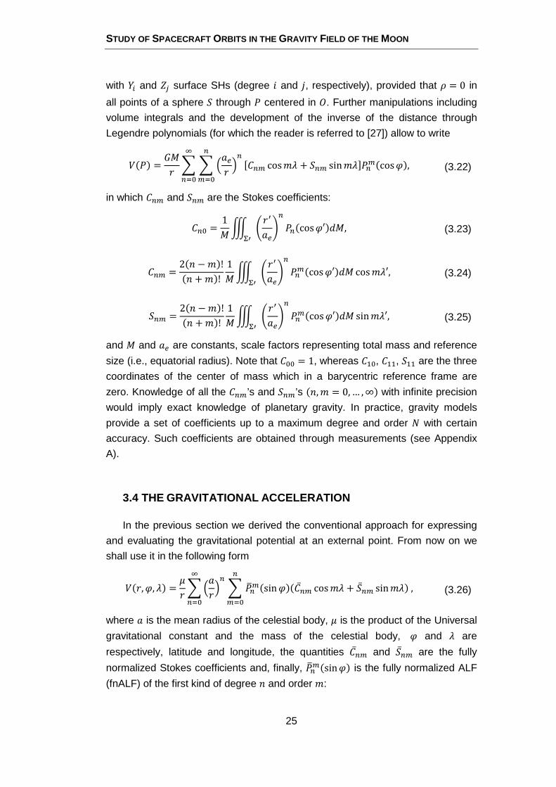
3.1 GRAVITATIONAL FIELD AND POTENTIAL THEORY .......................................................... 21
3.2 SPHERICAL HARMONICS ................................................................................................ 23
3.3 THE GRAVITATIONAL POTENTIAL IN SHS ........................................................................ 24
3.4 THE GRAVITATIONAL ACCELERATION ............................................................................ 25
3.5 PINES’ REPRESENTATION ............................................................................................... 26
CHAPTER FOUR. PERTURBATIONS ...................................................................................... 30
4.1 THIRD-BODY ................................................................................................................... 31
4.1.1 Earth-induced acceleration........................................................................................ 32
4.1.2 Sun-induced acceleration .......................................................................................... 33
4.2 SOLAR RADIATION PRESSURE ........................................................................................ 33
4.2.1 Eclipse conditions ...................................................................................................... 35
4.3 LUNAR ALBEDO .............................................................................................................. 36
4.4 LUNAR THERMAL RADIATION PRESSURE ....................................................................... 38
4.5 PERTURBATIONS AS A FUNCTION OF. ALTITUDE ........................................................... 39
CHAPTER FIVE. DEVELOPMENT OF THE CODE ....................................................................... 41
5.1 INPUT PARAMETERS ...................................................................................................... 41
5.1.1 Perturbation parameters ........................................................................................... 41
5.1.2 Initial position of the satellite .................................................................................... 42
5.1.3 Parameters related to integration ............................................................................. 44
5.1.4 Parameters related to celestial bodies ...................................................................... 45
E.CARDOSO
6
5.1.5 Other parameters ...................................................................................................... 45
5.2 OUTPUT PARAMETERS ................................................................................................... 46
5.3 CODE PERFORMANCE .................................................................................................... 47
5.3.1 Modifications and enhancements of the method of Pines ........................................ 49
5.3.2 Lumped coefficients synthesis of the geopotential and its gradients ........................ 52
5.3.1 Summary of the routines involved in the program .................................................... 54
CHAPTER SIX. SIMULATIONS .............................................................................................. 55
6.1 DEFINITION OF PARAMETERS ........................................................................................ 55
6.1.1 Integration steps ....................................................................................................... 55
6.1.2 Tolerance ................................................................................................................... 57
6.1.3 Output temporal resolution ....................................................................................... 57
6.2 VALIDATION OF THE CODE ............................................................................................. 58
6.2.1 Keplerian orbit ........................................................................................................... 58
6.2.2 Effect of �2 ................................................................................................................. 59
6.3 STUDY OF ORBITS ........................................................................................................... 61
6.4 SIMULATIONS ................................................................................................................ 63
6.4.1 Frozen orbits .............................................................................................................. 63
6.4.2 RGT lunar orbits ......................................................................................................... 69
6.4.3 Polar orbits ................................................................................................................ 72
CHAPTER SEVEN. CONCLUSIONS AND FUTURE WORK ......................................................... 78
APPENDIX A. LUNAR DATA............................................................................................ 80
A.1 LUNAR PROSPECTOR ..................................................................................................... 80
A.2 GRAVITY DATA ............................................................................................................... 82
APPENDIX B. MODEL PARAMETERS .............................................................................. 84
APPENDIX C. NUMERICAL SOLVER ................................................................................ 86
C.1 INTRODUCTION TO NUMERICAL ODE METHODS .......................................................... 86
C.2 RUNGE-KUTTA-FEHLBERG METHOD ............................................................................. 87
C.3 RUNGE-KUTTA-FEHLBERG METHOD OF ORDER 7(8) ..................................................... 87
APPENDIX D. BUDGET OF THE STUDY ............................................................................ 90
REFERENCES .............................................................................................................................. 92
BOOKS, LECTURES AND ARTICLES ............................................................................................... 92
WEBSITES .................................................................................................................................... 95
STUDY OF SPACECRAFT ORBITS IN THE GRAVITY FIELD OF THE MOON
7
LIST OF FIGURES
Fig. 1.1 Near and far sides views of the Moon (Extracted from [W5]) ............................................ 14
Fig. 1.2 Topography of the Moon as mapped from Clementine (Extracted from [W5]) ................. 15
Fig. 1.3 Vertical accelerations at the lunar surface expressed in mGal as mapped from LP with
mascons in red. J2 coefficients have been removed (Extracted from [18]) ............................ 15
Fig. 1.4 Images of the Luna 1 (left) and Pioneer 4 (right) probes .................................................... 16
Fig. 1.5 LP concept artist ................................................................................................................. 17
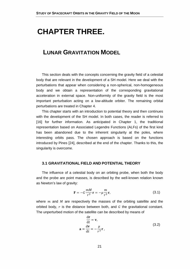
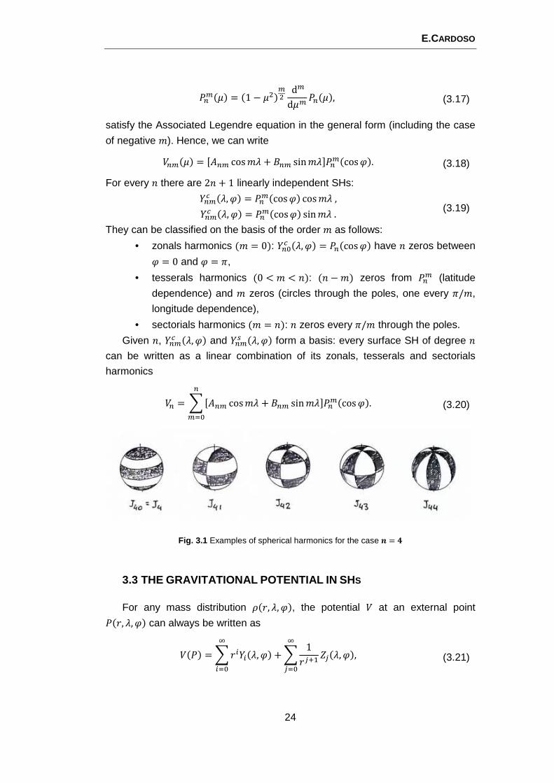
Fig. 3.1 Examples of spherical harmonics for the case � = 4 ......................................................... 24
Fig. 3.2 The global reference system (�, i1, i2, i3) and the local reference system (�, e1, e2, e3) . 27
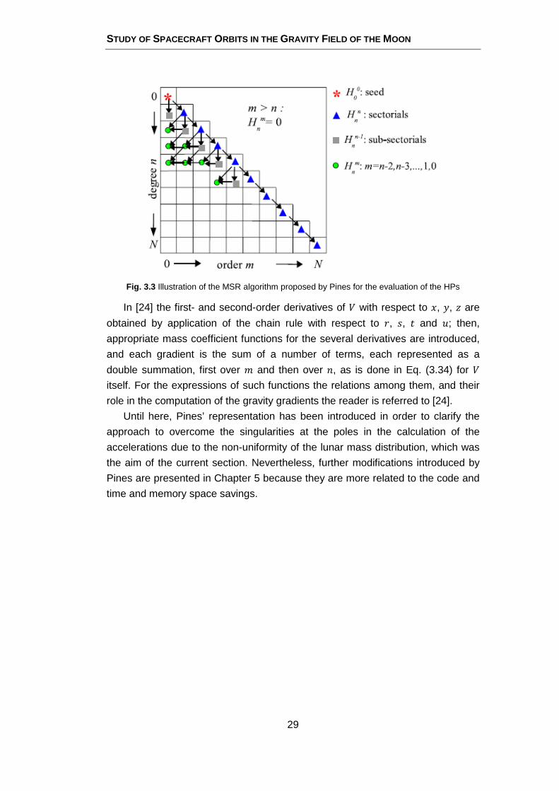
Fig. 3.3 Illustration of the MSR algorithm proposed by Pines for the evaluation of the HPs .......... 29
Fig. 4.1 Representation of the vectors in a three bodies system .................................................... 31
Fig. 4.2 Moon-Earth system with different geometric parameters ................................................ 32
Fig. 4.3 Representation of the eclipse zone with cylindrical shape ................................................ 36
Fig. 4.4 The angle between the Sun and the satellite pointing vectors defines the view factor
value ....................................................................................................................................... 38
Fig. 4.5 Accelerations due to each individual effect as altitude functions ...................................... 40
Fig. 5.1 Log10 of the difference between the fnHPs computed with the MSR algorithm and those
resulting from adopting the IDR scheme ................................................................................ 51
Fig. 5.2 Comparison between the IDR (left) and MSR (right) algorithm schemes........................... 51
Fig. 6.1 Evolution of orbital parameters within a whole orbit around the 347th
day in the
integration. In blue (ℎ = 1), in red (ℎ = 5) and in green (ℎ = 10) ........................................ 56
Fig. 6.2 Plane view of two orbits for different values of ‘ppo’: 10 (top left), 20 (top right), 30
(bottom left) and 40 (bottom right) ....................................................................................... 58
Fig. 6.3 Simulation of the Keplerian orbit (red) ............................................................................... 59
Fig. 6.4 Variation of the RAAN (left) and the argument of periapsis (right). The analytical effect
appears in green, the simulated results in blue ..................................................................... 60
Fig. 6.5 Variation of the RAAN (left) and the argument of periapsis (right) for an inclination of
63.435°. Analytical results appear in green, while the results of the simulations in blue ..... 61
Fig. 6.6 Evolution of the eccentricity over a 10 days interval for orbit F. Three simulations are
represented, corresponding to three different choices of the maximum degree and order
for the lunar gravity field: 10x10 (blue), 50x50 (red) and 100x100 (green) ........................... 64
Fig. 6.7 Evolution of the inclination over one orbital period for orbit F .......................................... 64
Fig. 6.8 Initial (in green) and final (in red) orbits for the 53 days interval of Orbit J ....................... 65
Fig. 6.9 Evolution of the orbital elements for Orbit J ...................................................................... 66
Fig. 6.10 Evolution of the orbital elements for Orbit D ................................................................... 67
Fig. 6.11 Evolution of the orbital elements for Orbit E ................................................................... 68
Fig. 6.12 Comparison of the results extracted from [26] (left) and simulation (right) for Orbit B .. 70
Fig. 6.13 Evolution of the orbital elements for Orbit B as extracted from [26] .............................. 70

E.CARDOSO
8
Fig. 6.14 Evolution of the orbital elements of Orbit B resulting from the simulations ................... 71
Fig. 6.15 3-D and 2-D graphics extracted from STK for Orbit B ....................................................... 72
Fig. 6.16 Coverage times (red) for Orbit B for a 4 days sample extracted from STK ....................... 72
Fig. 6.17 Constellation sample for achieving continuous coverage from a South Pole lunar base . 73
Fig. 6.18 Evolution of Orbit O (left) and Orbit P (right) with initial and final conditions shown
respectively in green and red ................................................................................................. 74
Fig. 6.19 Evolution of the orbital elements of Orbit O .................................................................... 75
Fig. 6.20 Evolution of the orbital elements of Orbit P ..................................................................... 76
Fig. 6.21 Two instant captures of the Orbit P passing over the same point for two different dates:
17th
December (left) and 14th
January (right). Extracted from STK ........................................ 77
STUDY OF SPACECRAFT ORBITS IN THE GRAVITY FIELD OF THE MOON
9
LIST OF TABLES
Table 5.1 Blocks of input parameters related to perturbations. In brackets are shown the values
used in the present study (see Appendix A) ........................................................................... 42
Table 5.2 Blocks of input parameters that give the initial position of the satellite ........................ 43
Table 5.3 Blocks of input parameters related to integration .......................................................... 45
Table 5.4 Block of input parameters related to celestial bodies ..................................................... 46
Table 5.5 Blocks of other input parameters .................................................................................... 46
Table 5.6 Different routines called by Pines.f90 and their tasks ..................................................... 49
Table 5.7 The several routines involved in the program and the task they perform ...................... 54
Table 6.1 Orbital parameters of the simulated satellite to study the effect of the integration step
................................................................................................................................................ 56
Table 6.2 Simulation elapsed time versus integration time step .................................................... 57
Table 6.3 Orbital elements employed in the simulation of a Keplerian orbit ................................. 59
Table 6.4 Initial orbital elements for the study of the �2 effect (� is the orbital period) ............... 60
Table 6.5 List of reference orbits found in the literature ................................................................ 61
Table 6.6 Time until lunar surface collision for low-altitude “frozen” orbits .................................. 65
Table 6.7 List of polar orbits analyzed in the present study ........................................................... 73
App. Table A.1 Different gravity models resulting from the LP tracking data................................. 82
App. Table B.1 Parameters related to the celestial bodies necessary for the study ....................... 84
App. Table B.2 Parameters related to the celestial bodies orbits necessary for the study ............ 84
App. Table B.3 Mass and area-to-mass ratios for different types’ satellites .................................. 85
App. Table C.1 Coefficients for the Runge-Kutta-Fehlberg 7(8) method ........................................ 89
App. Table D.1 HW and SW cost ..................................................................................................... 90
App. Table D.2 Worked hours cost .................................................................................................. 91
App. Table D.3 Total cost of the project ......................................................................................... 91

E.CARDOSO
10
LIST OF SYMBOLS
� Semi-major axis of an orbit
Mean radius of a celestial body
� Acceleration of the satellite with respect to the Moon center of mass
� Satellite’s front-side area
� Speed of light
�� Reflectivity of a surface element
��� Stokes coefficients of degree � and order �
� Eccentricity of an orbit
Gravitational acceleration
Universal gravitational constant
���� � Helmholtz Polynomial of degree � and order �
� Inclination of an orbit
�� Zonal harmonic coefficient of degree �
� Satellite’s mass
� Mass of a celestial body
� Mean motion
��� Full normalization factor for degree � and order �
���(�) Associated Legendre Functions of degree � and order �
� Position of the satellite with respect to the Moon center of mass
� Independent variable: time
�� Final time of integration
� Orbital period
Argument of latitude of an orbit
�� Solid spherical harmonic of degree �
�� Surface spherical harmonic of degree �
STUDY OF SPACECRAFT ORBITS IN THE GRAVITY FIELD OF THE MOON
11
� Gravitational potential
� Velocity of the satellite with respect to the Moon center of mass
� First coordinate of the position in a Cartesian reference frame
� Second coordinate of the position in a Cartesian reference frame
� Third coordinate of the position in a Cartesian reference frame
��� Kronecker’s delta
� True anomaly of an orbit
Longitude
� Gravitational parameter (� = �)
! Density
!� Parallactic factor of degree �
" Latitude
# Argument of periapsis of an orbit
Ω Right Ascension of the Ascending Node (RAAN) of an orbit
OPERATORS
$ Scalar magnitude
� Vector magnitude
�% First time derivative
�& Second time derivative
''� Total or full derivative with respect to �
((� Partial derivative with respect to �
∇$ Gradient of a scalar
�̅ Fully normalized coefficient
�*��� Fully normalized function or polynomial
E.CARDOSO
12
SUBSCRIPTS
� Degree of the SH expansion
� Order of the SH expansion
+�� Satellite
⨀ Sun
⊕ Earth
⊂ Moon
ACRONYMS
AD Atmospheric Drag
ALF Associated Legendre Functions
AL Atmospheric Lift
ARP Albedo Radiation Pressure
CM Center of Mass
DGE Doppler Gravity Experiment
DSN Deep Space Network
fnALF Fully normalized ALF
fnHP Fully normalized HP
GPS Global Positioning System
HP Helmholtz Polynomial
IDR Increasing Degree Recursion
LO Lunar Orbiter
LP Lunar Prospector
MSR Mixed Strides Recursion
NASA National Aeronautics and Space Administration
ODE Ordinary Differential Equations
PFS Particle & Fields Satellite
RAAN Right Ascension of the Ascending Node
STUDY OF SPACECRAFT ORBITS IN THE GRAVITY FIELD OF THE MOON
13
RGT Repeated Ground Tracks
RTBP Restricted Three-Bodies Problem
SH Spherical Harmonics
SRP Solar Radiation Pressure
STK Satellite Tool Kit
TRP Thermal Radiation Pressure
TB Third-Body gravitational perturbations
E.CARDOSO
14
CHAPTER ONE.
INTRODUCTION
Simulating an orbit in the vicinity of any celestial body is a classical
perturbations problem. The purely Keplerian dynamics is not sufficient to
accurately describe the motion of a spacecraft: important deviations from purely
elliptical orbits are caused by the real mass distribution within the body. It is worth
remembering that real space missions must be extremely precise. Moreover, the
closer a satellite is to a central body, the greater importance small effects take.
Such importance was clearly and dramatically shown by the case of PFS-2 in
1972, a probe released within the Apollo 16 mission. The Moon itself plunged the
subsatellite to its death by collision after a few orbits: the probe had been placed
in an unstable orbit, whose eccentricity was drastically modified by the
perturbative forces. [W1].
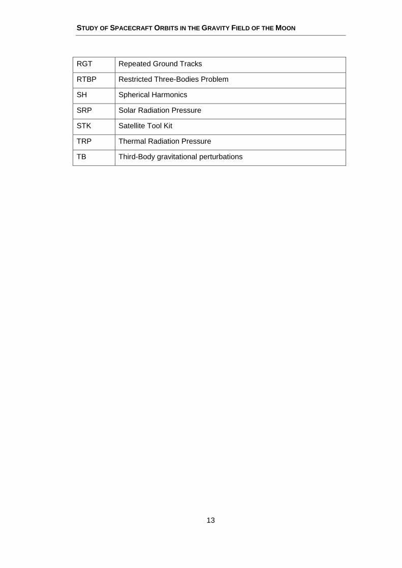
Fig. 1.1 Near and far sides views of the Moon (Extracted from [W5])
The Moon orbits the Earth in a 1:1 spin-orbit resonance at a mean distance
over 384000 km. As a result, it shows approximately always the same face to the
Earth1.
1 Note that the apparent wobble or variation in the visible side of the Moon, called libration, allows observers on Earth to see more than half of the lunar surface.
STUDY OF SPACECRAFT ORBITS IN THE GRAVITY FIELD OF THE MOON
15
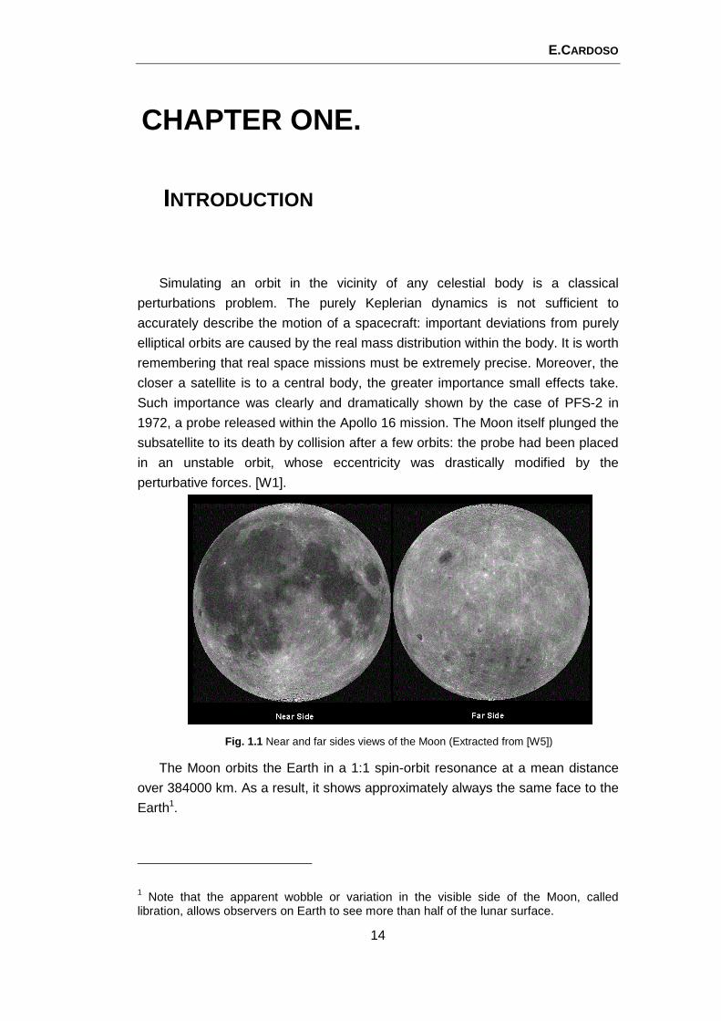
Fig. 1.2 Topography of the Moon as mapped from Clementine (Extracted from [W5])
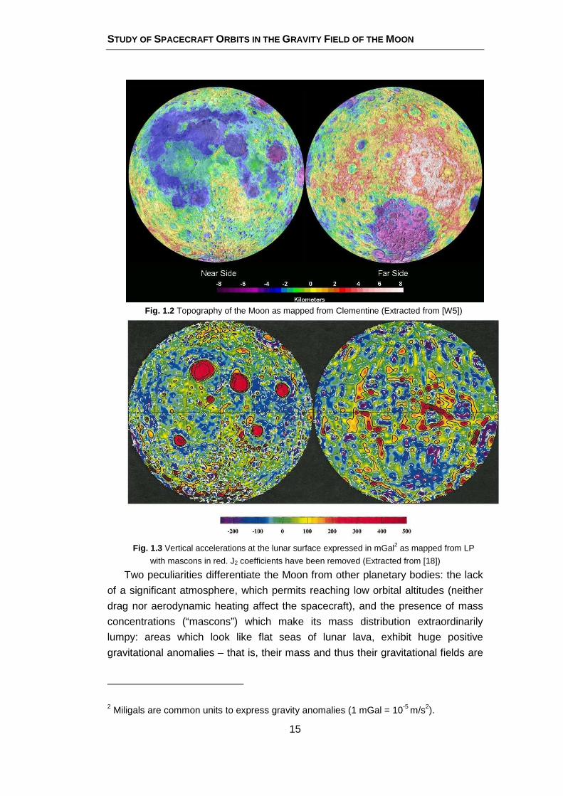
Fig. 1.3 Vertical accelerations at the lunar surface expressed in mGal2 as mapped from LP
with mascons in red. J2 coefficients have been removed (Extracted from [18])
Two peculiarities differentiate the Moon from other planetary bodies: the lack
of a significant atmosphere, which permits reaching low orbital altitudes (neither
drag nor aerodynamic heating affect the spacecraft), and the presence of mass
concentrations (“mascons”) which make its mass distribution extraordinarily
lumpy: areas which look like flat seas of lunar lava, exhibit huge positive
gravitational anomalies – that is, their mass and thus their gravitational fields are
2 Miligals are common units to express gravity anomalies (1 mGal = 10-5 m/s2).
E.CARDOSO
16
significantly stronger than the rest of the lunar crust. This phenomenon can be
appreciated by comparing Fig. 1.2 with Fig. 1.3.
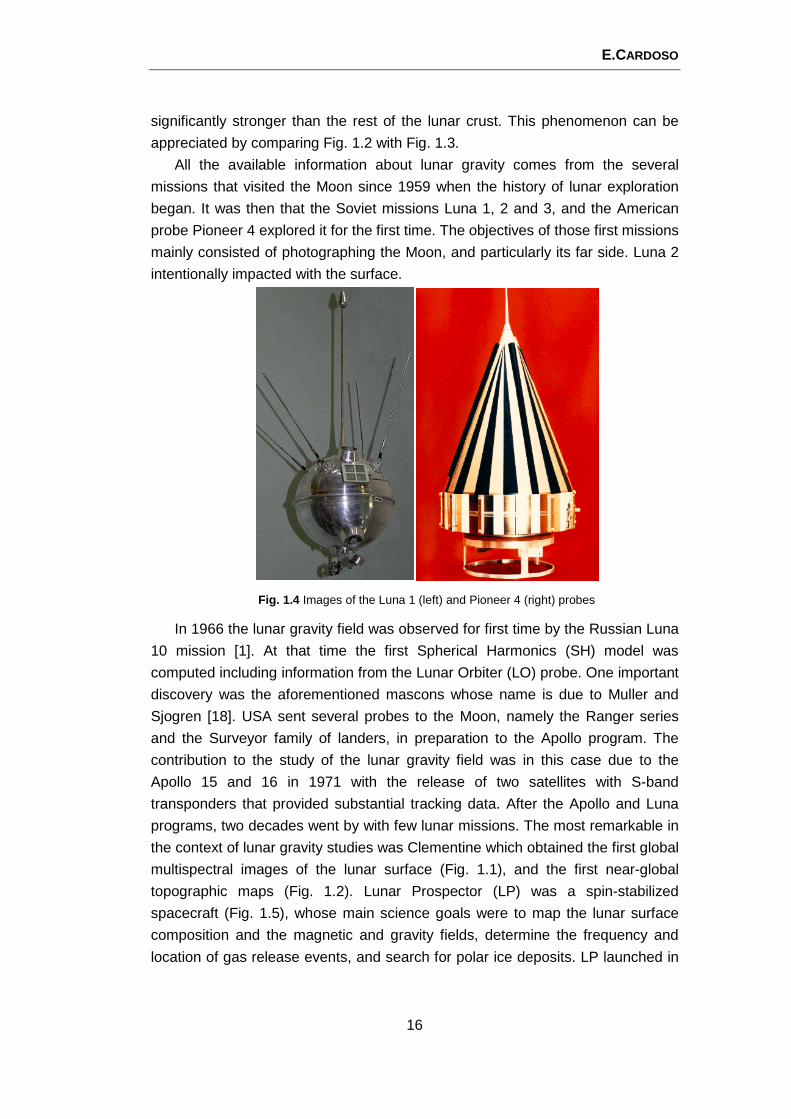
All the available information about lunar gravity comes from the several
missions that visited the Moon since 1959 when the history of lunar exploration
began. It was then that the Soviet missions Luna 1, 2 and 3, and the American
probe Pioneer 4 explored it for the first time. The objectives of those first missions
mainly consisted of photographing the Moon, and particularly its far side. Luna 2
intentionally impacted with the surface.
Fig. 1.4 Images of the Luna 1 (left) and Pioneer 4 (right) probes
In 1966 the lunar gravity field was observed for first time by the Russian Luna
10 mission [1]. At that time the first Spherical Harmonics (SH) model was
computed including information from the Lunar Orbiter (LO) probe. One important
discovery was the aforementioned mascons whose name is due to Muller and
Sjogren [18]. USA sent several probes to the Moon, namely the Ranger series
and the Surveyor family of landers, in preparation to the Apollo program. The
contribution to the study of the lunar gravity field was in this case due to the
Apollo 15 and 16 in 1971 with the release of two satellites with S-band
transponders that provided substantial tracking data. After the Apollo and Luna
programs, two decades went by with few lunar missions. The most remarkable in
the context of lunar gravity studies was Clementine which obtained the first global
multispectral images of the lunar surface (Fig. 1.1), and the first near-global
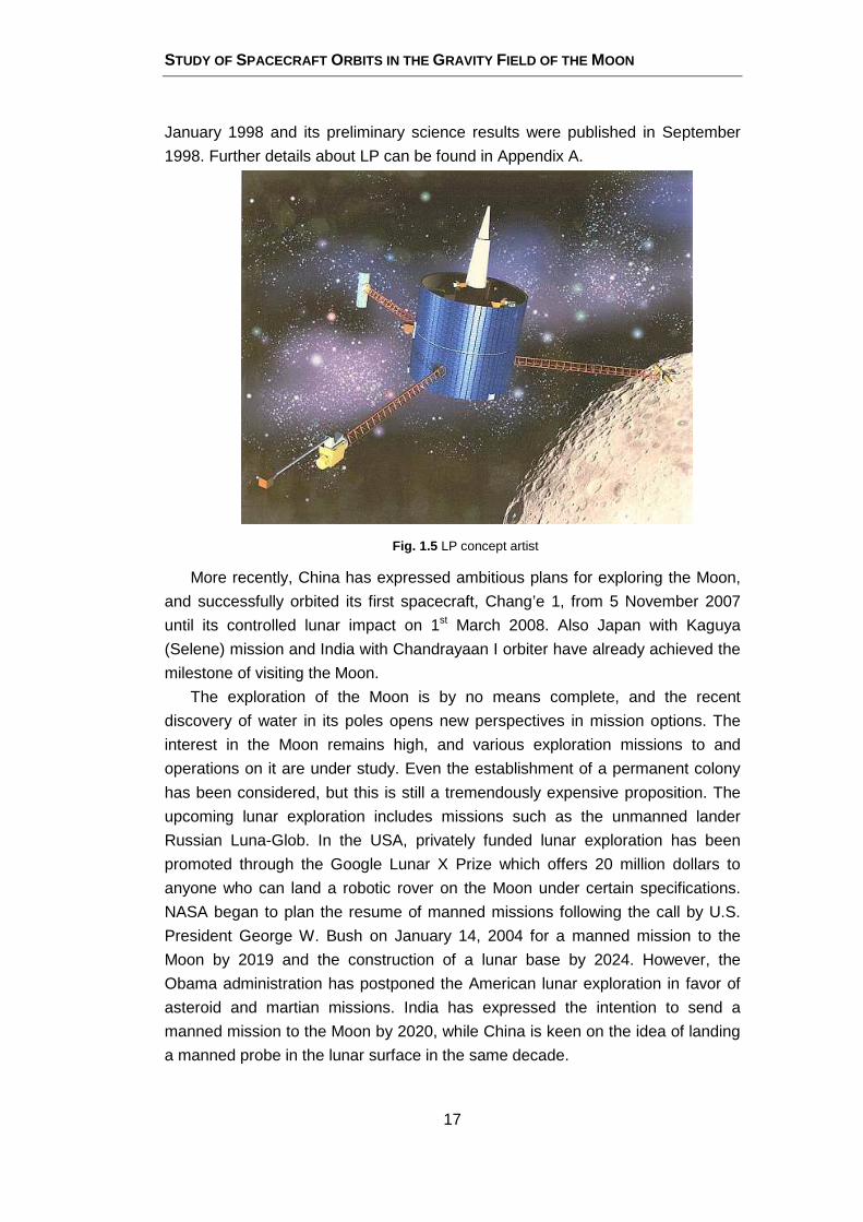
topographic maps (Fig. 1.2). Lunar Prospector (LP) was a spin-stabilized
spacecraft (Fig. 1.5), whose main science goals were to map the lunar surface
composition and the magnetic and gravity fields, determine the frequency and
location of gas release events, and search for polar ice deposits. LP launched in
STUDY OF SPACECRAFT ORBITS IN THE GRAVITY FIELD OF THE MOON
17
January 1998 and its preliminary science results were published in September
1998. Further details about LP can be found in Appendix A.
Fig. 1.5 LP concept artist
More recently, China has expressed ambitious plans for exploring the Moon,
and successfully orbited its first spacecraft, Chang’e 1, from 5 November 2007
until its controlled lunar impact on 1st March 2008. Also Japan with Kaguya
(Selene) mission and India with Chandrayaan I orbiter have already achieved the
milestone of visiting the Moon.
The exploration of the Moon is by no means complete, and the recent
discovery of water in its poles opens new perspectives in mission options. The
interest in the Moon remains high, and various exploration missions to and
operations on it are under study. Even the establishment of a permanent colony
has been considered, but this is still a tremendously expensive proposition. The
upcoming lunar exploration includes missions such as the unmanned lander
Russian Luna-Glob. In the USA, privately funded lunar exploration has been
promoted through the Google Lunar X Prize which offers 20 million dollars to
anyone who can land a robotic rover on the Moon under certain specifications.
NASA began to plan the resume of manned missions following the call by U.S.
President George W. Bush on January 14, 2004 for a manned mission to the
Moon by 2019 and the construction of a lunar base by 2024. However, the
Obama administration has postponed the American lunar exploration in favor of
asteroid and martian missions. India has expressed the intention to send a
manned mission to the Moon by 2020, while China is keen on the idea of landing
a manned probe in the lunar surface in the same decade.
E.CARDOSO
18
Navigation and telecommunications architectures constitute a major design
issue if a permanent manned colony is set on the Moon: a navigation
constellation of some extent would be a necessary infrastructure for locating
astronauts moving on the surface, especially during activities involving stays at
the far side, where no tracking from Earth is possible. Then, two or more
satellites could also provide permanent contact with the Earth. Scientific probes
are preferably positioned in low polar orbits where global coverage is naturally
obtained. Now, the information gathered by the above-listed historical missions
show that the Moon is a celestial body without a nearly regular surface,
moreover, its gravity field is non-uniform and exhibits significant anomalies.
Therefore, the dynamical stability and evolution of orbiting probes constitute a
critical design issue: the analysis of the orbital evolution of different types of
orbits, based on the available detailed knowledge of the lunar gravity field and
other physical sources of orbital perturbation can be employed in the choice of
the most suitable orbit for a given mission type and objective: the orbit/trajectory
is the physical basis on which the mission is built, its definition is closely related
to the payload design and to the mission objectives and top level requirements
[21]. Orbit suitability is related to lifetime and cost, and can be defined based on
the frequency and magnitude of the maneuvers required to maintain a given
geometry. Clearly, orbits which satisfy the mission objectives but require
minimum fuel usage are to be preferred. The consequences this has on the
design of the bus are important. Hence, to have a tool capable of simulating the
natural orbital evolution of a lunar satellite provides considerable aid in the
definition of the possible mission scenarios, including lifetime, propellant budget,
mass budget, observing strategy and operations.
The objective of the present study is to construct such analysis tool. Pseudo-
professional software is commercially available, most noticeably Satellite Tool Kit
(STK), a graphical 3D platform which performs simulations of orbital evolution
accompanied by visibility and communications architecture analysis. It has to be
said, however, that STK is by no means a research instrument, it is not open
source, the models it uses are not entirely documented and cannot be modified.
No code inspection is allowed and this limits the level of awareness on the
output. It offers very good support, though, and many of the simulations
presented in this report have been supplemented by information obtained with
STK.
The construction of the orbital evolution code has involved the modeling of
the gravitational acceleration at any point in outer space together with other
perturbing accelerations of relevant magnitude. The modeling of the gravity field
is based on potential theory, on the one hand, and lunar gravity data in the form
of spherical harmonics coefficients on the other. The traditional representation
based on Associated Legendre Functions of the first kind has been abandoned in
STUDY OF SPACECRAFT ORBITS IN THE GRAVITY FIELD OF THE MOON
19
favor of a different type of spherical harmonics representation in which the
involved functions depend on Cartesian coordinates and do not suffer from
singularities or loss of precision at the poles [24]. Then, an additional
improvement consisting in the implementation of the so-called lumped
coefficients in the treatment of the series expansions, allows considerable
memory and computing time savings over the traditional representation. When
the lunar gravitational acceleration is combined with the effect of third body and
radiation pressure perturbations, the resulting accelerations allow to predict the
motion of a close Moon satellite.
The present document is structured as follows: Chapter 2 contains the project
scope; Chapters 3 and 4 deal with the perturbation models, the former about the
central body, the latter the remaining perturbing sources. Chapter 5 illustrates the
development of the code that implements the functions and algorithms of the
previous chapters. Simulations of several interesting orbits are described and
commented in Chapter 6. Chapter 7 draws the conclusions of the study and
provides insight into its future developments.
E.CARDOSO
20
CHAPTER TWO.
PROJECT SCOPE
The scope of the project mainly consists in the extension of a Fortran code
developed by [5] which computes the gravitational potential of a planetary body
and its first-, second- and third-order gradients at any point in external space. The
extension includes
• the implementation of a Runge-Kutta-Fehlberg 7(8) numerical integrator
(see Appendix C)
• the implementation of the so-called lumped coefficients approach to the
series expansions of the central gravitational acceleration in order to
achieve better performance in memory usage and execution time (see
[13] and [14]).
• the rearrangement of the entire code in order to make it suitable to
simulating the orbital evolution of a low-altitude lunar probe under the
gravitational potential of the main body and other types of orbital
perturbations, namely third-bodies gravitational perturbations due to the
Sun and the Earth, and solar and thermal radiation pressures.
Then, the literature has been searched for orbits suitable for lunar missions of
different types. Simulations have been carried out in a context of mission
analysis: coverage, revisit time, durability and any other aspect related to orbital
evolution versus mission objective. Some results have been used to validate the
code by comparison with the literature, and STK has been adopted to
supplement the numerical simulations with geometrical information, such as the
visibility and the access times of interesting points on the surface.
Despite the fact that platform design is not the aim of the study, some
assumptions have been made concerning the main physical characteristics of the
satellite, namely mass, front section area, and reflectivity of the surface.
STUDY OF SPACECRAFT ORBITS IN THE GRAVITY FIELD OF THE MOON
21
CHAPTER THREE.
LUNAR GRAVITATION MODEL
This section deals with the concepts concerning the gravity field of a celestial
body that are relevant in the development of a SH model. Here we deal with the
perturbations that appear when considering a non-spherical, non-homogeneous
body and we obtain a representation of the corresponding gravitational
acceleration in external space. Non-uniformity of the gravity field is the most
important perturbation acting on a low-altitude orbiter. The remaining orbital
perturbations are treated in Chapter 4.
This chapter starts with an introduction to potential theory and then continues
with the development of the SH model. In both cases, the reader is referred to
[16] for further information. As anticipated in Chapter 1, the traditional
representation based on Associated Legendre Functions (ALFs) of the first kind
has been abandoned due to the inherent singularity at the poles, where
interesting orbits pass. The chosen approach is based on the functions
introduced by Pines [24], described at the end of the chapter. Thanks to this, the
singularity is overcome.
3.1 GRAVITATIONAL FIELD AND POTENTIAL THEORY
The influence of a celestial body on an orbiting probe, when both the body
and the probe are point masses, is described by the well-known relation known
as Newton’s law of gravity:
, = −��$� � = −� �$� �, (3.1)
where � and � are respectively the masses of the orbiting satellite and the
orbited body, $ is the distance between both, and the gravitational constant.
The unperturbed motion of the satellite can be described by means of d�d� = �,
� = d�d� = −
�$� �, (3.2)
E.CARDOSO
22
where � represents the position, � the velocity and a the acceleration of the
satellite with respect to the central body (� is a parallel to the line joining the
central body with the satellite).
The resulting motion is a Keplerian orbit: a circle, an ellipse, a parabola or a
hyperbola, the occurrence of one type or the others depending on the value of
the total mechanical energy.
Now, a real body is neither a point mass nor a perfect sphere (known to
behave in outer space like a point endowed with the same mass). So, the
gravitational potential � (and its gradients of any order) varies not only with the
distance to the satellite, but also with its position. The acceleration is the first-
order gradient of �,
� = ∇�. (3.3)
For a point mass,
� = �$ . (3.4)
And, for � negligibly small compared to �, Eqs. (3.3) and (3.4) are valid for a
coordinate system whose origin is at the center of mass (CM) of �. The
acceleration produced by several point masses �� at distances $� from m can be
expressed as the gradient of a potential which is the sum of potentials �� expressed by Eq. (3.4). If these particles form a continuous body of variable
density !, such summation is replaced by an integral over the volume of the
body:
� = .!(�,�, �)$(�,�, �) '�'�'�. (3.5)
In the case of a point mass, a specific component �� of � is given by
�� = (�(� = −� �$�, (3.6)
whereas the second gradient yields
��� = (�(� = �/− 1$� + 3�$ 0. (3.7)
which, summed to the remaining two diagonal elements of the second-order
gravity gradient tensor, provides the equation of Laplace:
∇� =(�(� + (�(� + (�(� = �/− 3$� + 3�� + � + ��$ 0 = 0. (3.8)
An equivalent result holds for any element of mass !'�'�'� in Eq. (3.5) and
hence for the summation thereof.
STUDY OF SPACECRAFT ORBITS IN THE GRAVITY FIELD OF THE MOON
23
3.2 SPHERICAL HARMONICS
A solid spherical harmonic ��(�,�, �) of degree � is every solution of the
Laplace’s equation that is positively homogeneous of degree � in �,�, �.
Changing to a system of spherical polar coordinates (a more appropriate choice
to describe the potential of a round body like a planet) 12$, ,"3, yields
����, �, �� = $���� ,"�. (3.9)
��� ,"� is a surface spherical harmonic of degree �. A given �� corresponds to
two solids SHs, ����, �, �� = $���� ,"� and ����,�, �� = $������� ,"� respectively of degree � and −� − 1.
The Laplacian in polar spherical coordinates takes the following form
1$ (�$���($ +
1$ sin" ((" 4sin" (��(" 5 + 1$ sin" (��( = 0. (3.10)
Substituting the definition of ��� ,"�, gives
1
sin" ((" 4sin" (��("5+ 1
sin" (��( + ��� + 1��� = 0. (3.11)
Then, we assume that �� can be written by separating the independent variables,
i.e., ��� ,"� = � ��"�. In the previous (3.9), this leads to the sum of two
independent terms. Such terms can be written as two opposite constants, i.e.,
��� + 1��1 − ��+ 1 − �Φ
d
d� 6�1 − ��dΦd� 7 = �, (3.12)
as latitude part and
1
ΛdΛ
d = −�, (3.13)
as azimuthal part, where � is an integer, called the order. The solution of Eq.
(3.13) is
� � = ���� +8���� , (3.14)
which in the real domain gives
Λ� � = � cos� + 9 sin� . (3.15)
The solution of Eq. (3.11) is ��� = 2� cos� + 9 sin� 3���"�, and it is a
surface SH of degree � and order �.
Eq. (3.12) is called Associated Legendre equation:
d
d� :�1 − �� d����d� ;+ :��� + 1� − �
1 − �; ���� = 0�|�| ≤ 1�. (3.16)
The ALFs of the first kind ���(�) of degree � and order �, defined as
E.CARDOSO
24
������ = �1 − ��� d�d�� �����, (3.17)
satisfy the Associated Legendre equation in the general form (including the case
of negative �). Hence, we can write
������ = 2��� cos� + 9�� sin� 3����cos"�. (3.18)
For every � there are 2� + 1 linearly independent SHs: =��� � ,"� = ����cos"� cos� , =��� � ,"� = ����cos"� sin� . (3.19)
They can be classified on the basis of the order � as follows:
• zonals harmonics (� = 0): =��� � ,"� = ���cos"� have � zeros between " = 0 and " = >,
• tesserals harmonics (0 < � < �): (� −�) zeros from ��� (latitude
dependence) and � zeros (circles through the poles, one every >/�,
longitude dependence),
• sectorials harmonics (� = �): � zeros every >/� through the poles.
Given �, =��� � ,"� and =��� � ,"� form a basis: every surface SH of degree �
can be written as a linear combination of its zonals, tesserals and sectorials
harmonics
�� = ?2��� cos� + 9�� sin� 3����cos"��
���
. (3.20)
Fig. 3.1 Examples of spherical harmonics for the case � = �
3.3 THE GRAVITATIONAL POTENTIAL IN SHS
For any mass distribution !�$, ,"�, the potential � at an external point ��$, ,"� can always be written as
���� =?$�=�� ,"��
���
+? 1$��� @�� ,"��
���
, (3.21)
STUDY OF SPACECRAFT ORBITS IN THE GRAVITY FIELD OF THE MOON
25
with =� and @� surface SHs (degree � and A, respectively), provided that ! = 0 in
all points of a sphere + through � centered in 1. Further manipulations including
volume integrals and the development of the inverse of the distance through
Legendre polynomials (for which the reader is referred to [27]) allow to write
���� = �$ ? ? B��$ C� 2��� cos� + +�� sin� 3����cos"�
�
���
�
���
, (3.22)
in which ��� and +�� are the Stokes coefficients:
��� = 1�. /$���0� ���cos"′�'�
��
, (3.23)
��� =2�� −��!�� +��! 1�. /$���0
� ����cos"′�'� cos� ′��
, (3.24)
+�� =2�� −��!�� +��! 1�. /$���0
� ����cos"′�'� sin� ′��
, (3.25)
and � and �� are constants, scale factors representing total mass and reference
size (i.e., equatorial radius). Note that ��� = 1, whereas ���, ���, +�� are the three
coordinates of the center of mass which in a barycentric reference frame are
zero. Knowledge of all the ���’s and +��’s ��,� = 0,… ,∞� with infinite precision
would imply exact knowledge of planetary gravity. In practice, gravity models
provide a set of coefficients up to a maximum degree and order � with certain
accuracy. Such coefficients are obtained through measurements (see Appendix
A).
3.4 THE GRAVITATIONAL ACCELERATION
In the previous section we derived the conventional approach for expressing
and evaluating the gravitational potential at an external point. From now on we
shall use it in the following form
��$,", � = �$ ?B�$C� ? �*���sin"����̅� cos� + +̅�� sin� ��
���
�
���
, (3.26)
where � is the mean radius of the celestial body, � is the product of the Universal
gravitational constant and the mass of the celestial body, " and are
respectively, latitude and longitude, the quantities ��̅� and +̅�� are the fully
normalized Stokes coefficients and, finally, �*���sin"� is the fully normalized ALF
(fnALF) of the first kind of degree � and order �:
E.CARDOSO
26
�*���sin"� = ��� :cos�"�! 2� d���
d�sin"���� �sin" − 1��;, (3.27)
with the full normalization factor
��� = D�2 − �����2� + 1� �� −��!�� +��!, (3.28)
where ��� is Kronecker’s delta. It is important to note that when the ALFs are fully
normalized, the stokes coefficients must be normalized accordingly.
The gravitational acceleration in an external point is the first-order gradient of
Eq. (3.26), which is also a SH expansion:
(�($ = −�$ ? ?�� + 1� B�$C
� ���̅� cos� + +̅�� sin� ��*���sin"��
���
�
���
, (3.29)
(�(" =�$ ? ? B�$C
� ���̅� cos� + +̅�� sin� �(�*���sin"�("�
���
�
���
, (3.30)
(�( = −�$ ? ? �B�$C
� ���̅� sin� − +̅�� cos� ��
���
�
���
�*���sin"�, (3.31)
3.5 PINES’ REPRESENTATION
Eqs. (3.26), (3.29), (3.30) and (3.31) are singular at the poles, with loss of
precision in the points nearby. This may constitute a serious drawback when
these accelerations are used to integrate the equations of motion of an orbiting
probe which may pass several times through the poles or near them. Alternative
SH representations allow to overcome this difficulty. The reader is referred to [5]
for a comparison of several methods for SH synthesis applied to the potential and
its first-, second- and third-order gradients. Among them, the method developed
by Pines ([24]) is based on a Cartesian representation of the SH functions and is
faster than the similar method of Cunningham & Metris ([7] and [23]): Both are
devoid of singularities at the geographic poles.
In Pines’ method the geopotential and its gradients are represented in terms
of so-called derived Legendre polynomials or Helmoltz Polynomials (HPs) in the
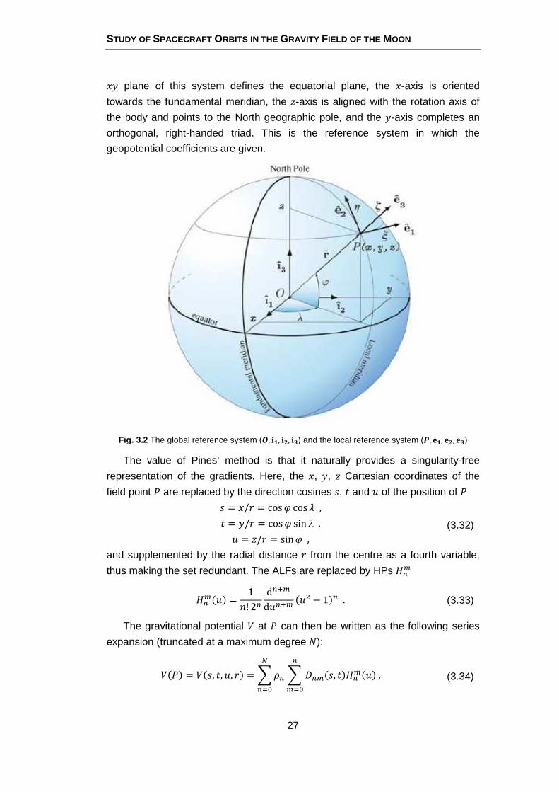
global reference system. This reference system is bodycentric (see Fig. 3.2), so it
has its origin 1 centered within the body and it is endowed with both the
Cartesian coordinate system (1, �, �, �) and the spherical equatorial coordinate
system (1, ,", $). The basis vectors E�, E, and E� form an orthonormal basis. The
STUDY OF SPACECRAFT ORBITS IN THE GRAVITY FIELD OF THE MOON
27
�� plane of this system defines the equatorial plane, the �-axis is oriented
towards the fundamental meridian, the �-axis is aligned with the rotation axis of
the body and points to the North geographic pole, and the �-axis completes an
orthogonal, right-handed triad. This is the reference system in which the
geopotential coefficients are given.
Fig. 3.2 The global reference system (�, ��, ��, ��) and the local reference system (�, ��, ��,��)
The value of Pines’ method is that it naturally provides a singularity-free
representation of the gradients. Here, the �, �, � Cartesian coordinates of the
field point � are replaced by the direction cosines F, � and of the position of � F = �/$ = cos" cos , � = �/$ = cos" sin , = �/$ = sin", (3.32)
and supplemented by the radial distance $ from the centre as a fourth variable,
thus making the set redundant. The ALFs are replaced by HPs ���
���� � = 1�! 2� d���
d ��� � − 1��. (3.33)
The gravitational potential � at � can then be written as the following series
expansion (truncated at a maximum degree �):
���� = ��F, �, , $� = ?!� ? 8���F, ������ ��
���
�
���
, (3.34)
E.CARDOSO
28
where the parallactic factor !� = �/$(�/$)� is computed recursively through
!� = B�$C !���, !� = �$ ,� = 1,2,…�, (3.35)
and 8���F, �� is called the “mass coefficient function” of degree � and order �
8���F, �� = ���$��F, �� + +�����F, ��. (3.36)
The functions $��F, �� and ���F, �� are defined as $��F, �� = Re�F + ����, ���F, �� = Im�F + ����, (3.37)
where
�F + ���� = �cos" cos + � cos" sin �� = ��� cos�". (3.38)
$� and �� with � = 0,1,… ,� are determined recursively with $� = F$��� − �����, �� = F���� + �$���, (3.39)
after initialization with $� = 1, �� = 0. In this procedure, the cos� " factor, which is
responsible for the singularities in the derivatives of the fnALFs at the geographic
poles, is no longer bound to the SH function, but to $� and ��, which are never
singular. This makes the gradients of � with respect to " singularity-free.
In the method of Pines the sectorial HP are determined by means of an
increasing degree-and-order recursion on the sectorial terms (i.e., � = � with � ≥ 1):
���� � = �2� − 1�����
���� �, (3.40)
Initialized with ���� � = 1 (which follows from �� = 1). The sub-diagonal elements
(zonals and tesserals with � = � − 1 and � ≥ 1) are obtained through the
recursion
������ � = ��
�� �. (3.41)
The remaining zonal and tesserals terms (0 ≤ � ≤ � − 2) are computed through
a mixed-strides recursion (MSR) formula:
���� � = 2 ��
���� �−�������( )3/(� −�), (3.42)
whereas, by definition,
���� � = 0, � > �. (3.43)
The computation procedure is represented in Fig. 3.3. In lower triangular part of
the matrix, every square correspond specific combination of � and �. Away from
the diagonal ��� is a linear combination of polynomials of different degree/order,
therefore not on the same stride (row/column).
STUDY OF SPACECRAFT ORBITS IN THE GRAVITY FIELD OF THE MOON
29
Fig. 3.3 Illustration of the MSR algorithm proposed by Pines for the evaluation of the HPs
In [24] the first- and second-order derivatives of � with respect to �, �, � are
obtained by application of the chain rule with respect to $, F, � and ; then,
appropriate mass coefficient functions for the several derivatives are introduced,
and each gradient is the sum of a number of terms, each represented as a
double summation, first over � and then over �, as is done in Eq. (3.34) for �
itself. For the expressions of such functions the relations among them, and their
role in the computation of the gravity gradients the reader is referred to [24].
Until here, Pines’ representation has been introduced in order to clarify the
approach to overcome the singularities at the poles in the calculation of the
accelerations due to the non-uniformity of the lunar mass distribution, which was
the aim of the current section. Nevertheless, further modifications introduced by
Pines are presented in Chapter 5 because they are more related to the code and
time and memory space savings.
E.CARDOSO
30
CHAPTER FOUR.
PERTURBATIONS
In this chapter we deal with the remaining orbital perturbations that may affect
a low-altitude lunar orbiting satellite. Here is a complete list of the effects that
need to be evaluated and, in case, taken into account ([3], [6], [8], and [28]):
• Atmospheric drag (AD)
• Atmospheric lift (AL)
• Third-body gravitational perturbations (TB)
• Solar radiation pressure (SRP)
• Albedo radiation pressure (ARP) of the central body
• Thermal radiation pressure (TRP) of the central body
• Tides
• Magnetic field
• Propulsion system’s thrust
The Moon does not possess a significant atmosphere3: the small amount of
atmospheric gases does not constitute a relevant source of orbital perturbation.
Hence, both AD and AL can be neglected.
The magnitude of the tidal effects on artificial satellites is very small. Despite
playing an important role in the evolution of the massive satellites of Jupiter,
Saturn, and other outer planets, it is usually not included in the perturbation
equations [6]. So, its contribution has not been taken into account in the present
study.
The Moon has a residual, crustal magnetic field of intensity between 1 and
100 nT, less than one-hundredth that of the Earth; it does not exhibit a global
dipolar magnetic field, as would be generated by a liquid metal core geodynamo,
and the external magnetization was probably acquired early in lunar history when
a geodynamo was still operating [12].
Thrusts of the engine constitute a large perturbation, but it is a planned and
known one, and, furthermore, here we do not deal with orbital maneuvers
3 Lunar atmospheric pressure is far less than 1 · 10���[���] and it contains approximately 80.000 atoms per cubic centimeter (Argon and Helium in more than 99%).
STUDY OF SPACECRAFT ORBITS IN THE GRAVITY FIELD OF THE MOON
31
because we are interested in observing and exploiting the free evolution of the
orbit. So, this effect is not considered.
Sections 4.1 to 4.4 derive the general treatment for the remaining orbital
perturbations in the above list, and obtain the corresponding accelerations, to be
added in Eq.(3.2) leading to:
� = d�d� = −
�$� �+ �����. (4.1)
where ����� are the perturbative accelerations determined in each section. Each
section includes the description of the model and the assumptions on which they
are based. Finally, Section 4.5 discusses the relative magnitude of the various
effects as a function of altitude.
4.1 THIRD-BODY
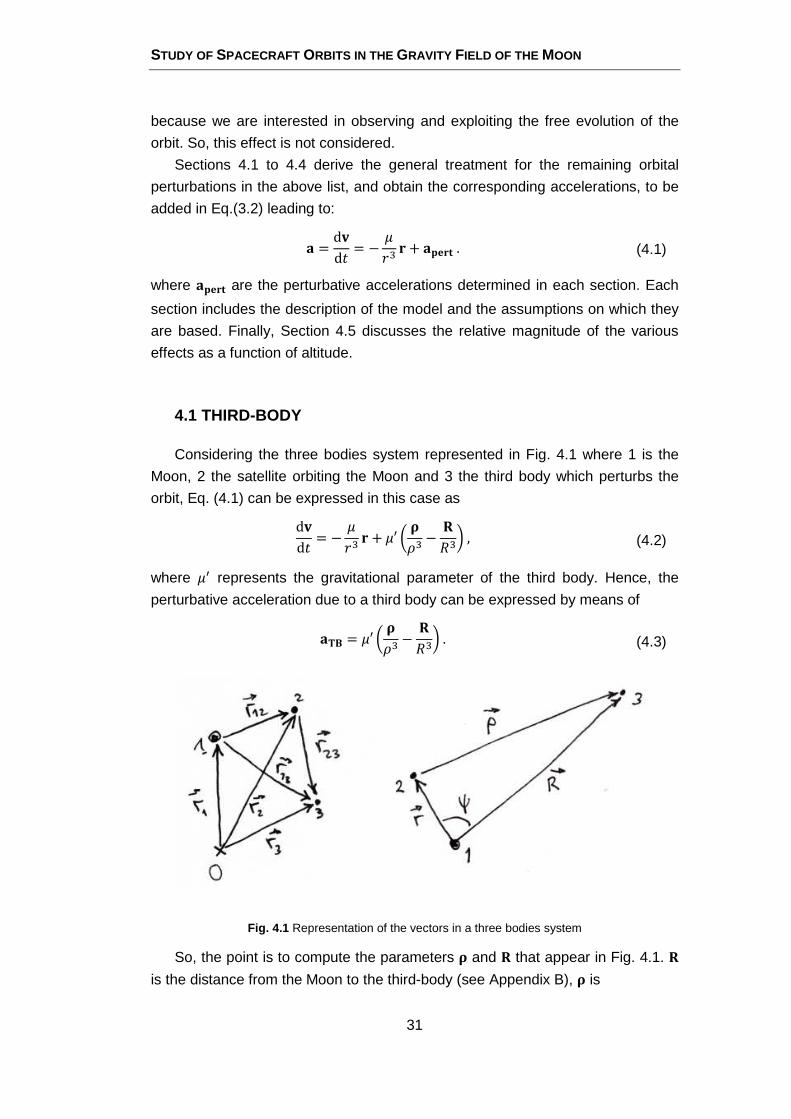
Considering the three bodies system represented in Fig. 4.1 where 1 is the
Moon, 2 the satellite orbiting the Moon and 3 the third body which perturbs the
orbit, Eq. (4.1) can be expressed in this case as
d�d� = −
�$� �+ �′ 4 G!� − HI�5, (4.2)
where �� represents the gravitational parameter of the third body. Hence, the
perturbative acceleration due to a third body can be expressed by means of
��� = �′ 4 G!� − HI�5. (4.3)
Fig. 4.1 Representation of the vectors in a three bodies system
So, the point is to compute the parameters G and H that appear in Fig. 4.1. H
is the distance from the Moon to the third-body (see Appendix B), G is
E.CARDOSO
32
G = H− �. (4.4)
The Sun and the Earth constitute the only relevant contributors to this
perturbation at the Moon, exactly like the Sun and the Moon are the only
significant third bodies at the Earth [6]. Furthermore, we assume that the Sun, the
Earth and the Moon lie in a common plane and their orbits are circular (and we
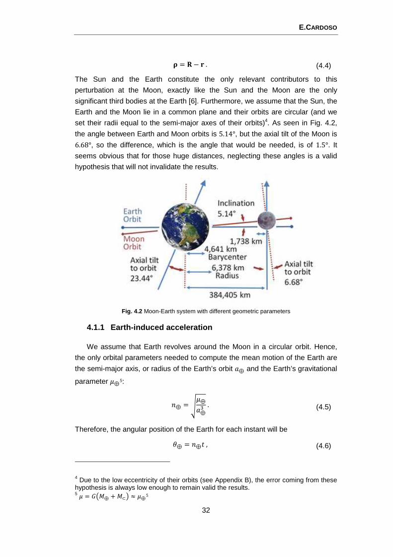
set their radii equal to the semi-major axes of their orbits)4. As seen in Fig. 4.2,
the angle between Earth and Moon orbits is 5.14°, but the axial tilt of the Moon is
6.68°, so the difference, which is the angle that would be needed, is of 1.5°. It
seems obvious that for those huge distances, neglecting these angles is a valid
hypothesis that will not invalidate the results.
Fig. 4.2 Moon-Earth system with different geometric parameters
4.1.1 Earth-induced acceleration
We assume that Earth revolves around the Moon in a circular orbit. Hence,
the only orbital parameters needed to compute the mean motion of the Earth are
the semi-major axis, or radius of the Earth’s orbit �⊕ and the Earth’s gravitational
parameter �⊕5:
�⊕ = D�⊕�⊕� . (4.5)
Therefore, the angular position of the Earth for each instant will be
�⊕ = �⊕�, (4.6)
4 Due to the low eccentricity of their orbits (see Appendix B), the error coming from these hypothesis is always low enough to remain valid the results. 5 = �� ⊕ + ⊂� ≈ ⊕5
STUDY OF SPACECRAFT ORBITS IN THE GRAVITY FIELD OF THE MOON
33
where we set �⊕�� = 0� = 0. Hence, the position of the Earth with respect to the
Moon is
�⊕⊂ = �⊕Jcos�⊕ , sin�⊕K. (4.7)
Now, substituting in Eq. (4.4), yields:
G⊕ = �⊂⊕ − � = −�⊕⊂ − �. (4.8)
Eventually, the perturbative acceleration due to the Earth is
���,⊕ = �⊕ 4G⊕!� − �⊂⊕I�5. (4.9)
4.1.2 Sun-induced acceleration
For the case of the Sun, the procedure is the same, with the only difference
consisting in the composition of the orbital motion of the Sun around the Earth
and that of the Earth around the Moon:
�⨀ = D�⨀�⨀� . (4.10)
�⨀ = �⨀�, (4.11)
�⨀⊕ = �⨀�cos�⨀ , sin�⨀�. (4.12)
Now, the position of the Sun relative to the Moon is
�⨀⊂ = �⨀⊕ + �⊕⊂, (4.13)
and substituting again in Eq. (4.4), we obtain:
G⨀ = �⊂⨀ − � = −�⨀⊂ − �. (4.14)
Thus, the perturbative acceleration for the case of the Sun is:
���,⨀ = �⨀ 4G⨀!� − �⊂⨀I�5. (4.15)
4.2 SOLAR RADIATION PRESSURE
The pressure of the solar radiation produces a non-conservative perturbation,
an acceleration resulting from the momentum exchange between the photons
and the surface of the satellite. SRP depends on the distance from the Sun
(through the value of the radiation flux), the area-to-mass ratio and the reflectivity
properties of the surface. One of the difficulties in analyzing this effect is
E.CARDOSO
34
accurately modeling the solar cycle and its variations, as part of the solar flux.
Similarly, the cross-sectional area and any shadowing effects on the spacecraft
itself are difficult to determine: since the incoming radiation from the Sun exerts a
force on the satellite, the effective surface of the satellite as seen from the Sun is
crucial in accurately estimating the amount of acceleration.
The pressure is simply the force divided by the incident area exposed to the
Sun. This means that the pressure distribution is critical, and this depends on the
satellite’s shape and composition. Incorporating the mass, allows to transform
from force to acceleration. However, this entire process involves determining the
Sun’s location, the satellite orbital attitude, the solar radiation pressure, the
effective, time-varying cross-sectional area exposed to the incoming radiation,
and the usually time-varying coefficients that model the satellite’s reflectivity. In
order to simplify, some assumptions must be made.
We start with the intensity of the energy: at the distance of 1 AU from the
Sun, the solar-radiation constant, or intensity, or irradiance, or solar flux, is +L = 1367M/� (see Appendix B). Most analyses use this value for the solar
constant because determining the actual frequencies and energy is very difficult.
Then, the pressure, or amount of momentum imparted, is given by
N�� = +L� =1367M/�
3 · 10 �/F = 4.57 · 10�!��
(4.16)
Now, using the reflectivity ��, the solar-radiation pressure N�� and the exposed
area to the Sun �⊙, the imparted force is
,"# = −N�����⨀� (4.17)
The reflectivity indicates how the satellite reacts to the interaction with the
photons and it is always between 0 and 2: 0 means that the surface is
translucent, no force is imparted, but there may be some refraction; a value of 1
means that all the radiation is absorbed, a value of 2 indicates that all the
radiation is specularly reflected (e.g., a flat mirror perpendicular to the light
source). It turns out that determining �� properly is extremely difficult. It changes
over time and is virtually impossible to predict. This is especially true for complex
satellites made of various materials, which enter and exit eclipse regions, and
have a constantly changing orientation. For this reason, it is almost always a
solution parameter, determined by differential correction. It is common to assume
that the surface maintains a constant attitude and stays oriented orthogonally to
the Sun. Though not very realistic, this assumption provides acceptable
estimates for the effect of the solar radiation pressure.
Newton’s second law allows to determine the acceleration with the given
force:
STUDY OF SPACECRAFT ORBITS IN THE GRAVITY FIELD OF THE MOON
35
��� = L��� =N�����⨀� (4.18)
Because the direction of �"# is always away from the Sun, a unit vector from the
satellite to the Sun yields the correct direction. The formula commonly used for
numerical simulations is:
�"#$ = −N�����⨀� �%&�⨀O�%&�⨀O = −N���� �� �%&�⨀O�%&�⨀O (4.19)
with �/� representing the area-to-mass ratio (see Appendix B). In this equation
several assumptions were made concerning satellite attitude and other
parameters. Satellites have complex geometries. Some surfaces reflect diffusely;
others reflect specularly and with changing aspect toward the Sun. Hence, at any
moment, the satellite will experience a net force, in general not directed as the
Sun-satellite vector, plus a torque. This introduces the possibility of implementing
the so-called solar sail in which solar-radiation pressure becomes the “wind” to
move the satellite in a “low-thrust-like” maneuver. Because the interest is on
orbital motion, the torque is often ignored and the disturbing acceleration is given
through Eq. (4.19), where �⊙ is an average effective cross-section that implicitly
incorporates ��. The subscript, which means that the area referred is the one
facing the Sun, has been suppressed as a simplification. As all radiative effects
depend on the product of the reflectivity and the area-to-mass ratio, with different
areas and reflectivities, but generally similar values, one value for this parameter
has been chosen (see Appendix B) and has been used for all the perturbations of
this kind.
In reality, though, the reflection process is two-fold: absorption followed by
reflection. Nevertheless, as its effect has minor importance for the case of study,
as it will be showed in Section 4.4, Eq. (4.19) is considered adequate for
obtaining the perturbative acceleration due to SRP.
4.2.1 Eclipse conditions
SRP only affects the satellite in the illuminated parts of its orbit: if the Earth or
the Moon eclipse the satellite, the perturbation due to SRP is null. In order to
determine if the satellite is eclipsed, we use the relative positions of Sun, Earth
and Moon as determined in Section 4.1. The shadow zone is considered
cylindrical (Fig. 4.3): this implies that the satellite is eclipsed by the given body
(the Moon or the Earth) when
O��'( × P⨀O = $ sinQ < I, (4.20)
��'( · P⨀ = $ cosQ < 0. (4.21)
E.CARDOSO
36
��'( · P⨀ = $ cosQ < 0, (4.22)
in which P⨀ and ��'( are vectors with origin in the given body: P⨀ is a unit vector
to the Sun, whereas ��'( is the relative position of the satellite. I is the radius of
the central body, and Q is the angle between the two vectors (Fig. 4.4).
Fig. 4.3 Representation of the eclipse zone with cylindrical shape
So, for the case of the Earth the vectors will be determined as follows:
P⨀ = P⊕⨀ = �⊕⨀O�⊕⨀O, (4.23)
��'( = �⊕�'( = �⊕⊂ + �, (4.24)
and for the Moon:
P⨀ = P⊂⨀ = �⊂⨀O�⊂⨀O, (4.25)
��'( = �, (4.26)
When both conditions (4.20) and (4.21) are met for one or both bodies (Moon
or Earth), the satellite is in eclipse and SRP does not contribute to the
perturbative acceleration, so the value of Eq (4.19) is zero.
4.3 LUNAR ALBEDO
Solar radiation that reflects off a celestial body is called albedo. The
magnitude of its effect on an orbiting satellite is much more difficult to model than
the SRP or the thermal radiation pressure because it depends on the relative
position between the satellite, the Moon and the Sun through the so-called view
factors. It also depends on the orbital altitude, i.e. the distance between the
satellite and the source of the perturbation.
STUDY OF SPACECRAFT ORBITS IN THE GRAVITY FIELD OF THE MOON
37
The amount of reflected radiation by the Moon is about 7% (see Appendix B)
of the incoming solar radiation and its effect on some satellites can be
measurable.
The acceleration produced by the ARP is modeled by taking into account that
only the illuminated side of the Moon contributes to this effect. Furthermore, each
illuminated elementary element on the surface contributes in a different way
depending on the how they are oriented with respect to each elementary surface
of the satellite. In practice, latitude-longitude regions define central locations that
produce individual accelerations. Denser grids produce more accurate results,
but at the cost of significantly higher processing times. The acceleration due to
ARP can be described as
�)#$ = −??N*���,����� �%&�⊂,��O�%&�⊂,��O��
(4.27)
in which subscript � indicates the generic satellite element, A refers to the surface
element on the Moon, N*� is the albedo radiation pressure, ��,� is the reflectivity
of the satellite’s surface element �, ��� is the area of a generic element � in the
satellite illuminated by a surface element A of the Moon, � is the mass of the
satellite, and �%&�⊂,�� is the relative position of the generic element with respect to
the lunar surface element. The area and the direction vary for each Moon location A considered. A way to simplify the treatment is by means of the radiative flux due
to albedo:
�*� = � · +L · L, (4.28)
Where � is the planetary albedo coefficient, 0.07 for the Moon as
aforementioned, and L is the view factor which depends on the incident angle
and can be computes by means of tables or graphics. Then, the radiation
pressure becomes
N*� = �*�� (4.29)
thus, giving a simplified relation for the perturbative acceleration due to lunar
albedo:
�)#$ = N*����⊂� �%&�⊂|�%&�⊂| = N*��� �� �%&�⊂|�%&�⊂| (4.30)
Note that in Eq. (4.30) the view factor is contained in the pressure radiation
parameter, but the computing way results easier than in Eq. (4.27). This view
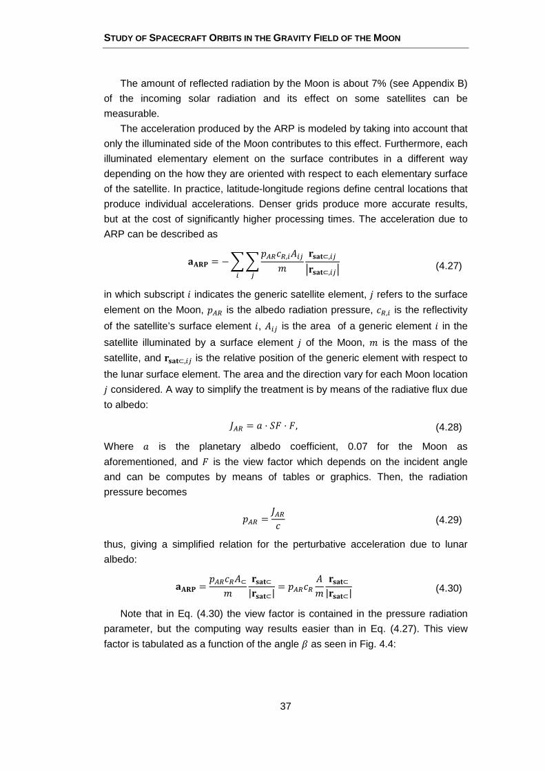
factor is tabulated as a function of the angle Q as seen in Fig. 4.4:
E.CARDOSO
38
Fig. 4.4 The angle between the Sun and the satellite pointing vectors defines the view factor value
4.4 LUNAR THERMAL RADIATION PRESSURE
The radiation environment in the vicinity of the Moon includes the direct solar
radiation, the surface albedo and the thermal radiation emitted in the infrared by
the surface. Important differences in temperature exist between night (−153[℃]) and day (107[℃]) on the Moon (the lack of an atmosphere does not mitigate the
diurnal thermal gradients). Such temperature difference produces dramatically
different emitted fluxes between day (1400 W/m2) and night side (a few W/m2).
For practical purposes and considering the short orbital periods relative to the
thermal inertia of the spacecraft, one can assume that the Moon radiates an IR
flux equal to the average value measured at some given phase on the illuminated
side: �+, = 977[M/�] (see [22]) Furthermore, it is reasonable to assume that
thermal radiation emanates uniformly. The intensity of this radiation decreases
with altitude as
�+� = 977 4I⊂|�|5
, (4.31)
where I⊂ is the lunar radius. Eventually, the thermal lunar radiation pressure is
obtained as in Eq. (4.16):
N+� = �+,� (4.32)
The perturbative acceleration of this effect can be computed also as in Eq. (4.19):
��#$ = −N+����⊂� �%&�⊂|�%&�⊂| = −N+��� �� �%&�⊂|�%&�⊂| (4.33)
The precise computation of the acceleration produced by the thermal radiation
pressure requires the evaluation of the exact amount of flux received by the
satellite. This flux depends on the relative orientation among the three bodies and
STUDY OF SPACECRAFT ORBITS IN THE GRAVITY FIELD OF THE MOON
39
therefore it involves once again the computation of the visibility factors as in the
case of the albedo flux.
4.5 PERTURBATIONS AS A FUNCTION OF. ALTITUDE
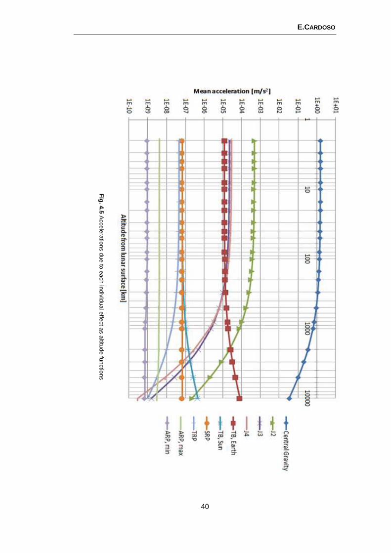
We conclude by evaluating the mean acceleration due to each perturbation
considered as acting separately on the satellite. We study the behavior as a
function of altitude from the lunar surface. Fig. 4.5 illustrates the average effects
of TB (Sun and Earth), solar radiation pressure, lunar thermal radiation pressure,
and the higher-order zonal harmonics of the gravity field (J2, J3, J4) against the
central Keplerian term. For the albedo, the maximum and the minimum appear,
instead of the average, the reason being that the use of values from a graph for
the view factors reduces the precision.
In the figure we find confirmation that the non-uniformity of the gravity field
constitutes the main perturbation at low altitudes, up to 2000 km, where the third-
body effect of the Earth becomes dominant. As expected, the lunar gravitational
and thermal effects decrease with the altitude, while those associated to the third
body increase. The albedo effects stay always between four and five magnitude
orders of magnitude below the largest acceleration. For this reason, the albedo
has been excluded from the model.
E.CARDOSO
40
Fig. 4.5
Accelerations due to each individual effect as altitude functions
STUDY OF SPACECRAFT ORBITS IN THE GRAVITY FIELD OF THE MOON
41
CHAPTER FIVE.
DEVELOPMENT OF THE CODE
The objective of this study is to develop a tool to analyze the evolution of low
lunar orbits. For this purpose, the original Fortran90 code mentioned in Chapter 2
has been modified: it now computes such evolution under several orbital effects.
The present chapter is dedicated to the structure of the code.
The main building blocks are the numerical integrator, a Runge-Kutta-
Fehlberg 7(8), and the several accelerations. The latter are determined as
described in Chapters 3 and 4. The numerical integration of the equations of
motion returns the position of the satellite at successive steps, and at each new
position the acceleration is computed and used in the subsequent integration.
This chapter starts with the description of the input parameters (Section 5.1),
followed by the illustration of the output (Section 5.2). Section 0 is dedicated to
the performance of the tool with particular emphasis on the lumped coefficients
method. The interested reader can access the code in the Annex A.
5.1 INPUT PARAMETERS
The input parameters are divided into five categories:
• Parameters related to perturbations
• Initial position of the satellite
• Parameters related to integration
• Parameters related to the celestial bodies
• Others
The values of the several parameters are introduced into the code through a
text file named “input_Orbit_Integration.txt”.
5.1.1 Perturbation parameters
The parameters related to the perturbations are listed in Table 5.1: there is a
set of four booleans that decide which perturbations have to be included: TB from
Earth and Sun, SRP and TRP (see Chapter 4). Each perturbation can be
selected independently: if selected, its contribution is added to the acceleration
vector. The lunar gravity field is treated separately. Two blocks allow its
E.CARDOSO
42
modification: one is about the specific model used and the other defines the
portion of the model to be used (i.e., maximum degree N_max and order
M_max). The different harmonic terms can be taken into account by modifying
these two blocks. Hence, the relative effect of different harmonics can be studied
by considering different field portions and forcing pre-selected coefficients to be
zero. For example, if one wants to quantify the effect of a certain harmonic, e.g.:
the third one (� = 3, � = 0), all the terms must be zero, except ��̅� and the
central gravity term (��̅�). Then, the contribution of the central gravity term must
be subtracted and the acceleration resulting will be the one due to the third zonal
harmonic.
It is important to note that the central gravity term (represented by the term ��̅� = 1) must always be included because it is not a perturbation and it allows to
obtain a regular orbit. The terms ��̅�, ��̅�, +̅�� are all zero because the reference
frame adopted is a barycentric one (see Chapter 3). The upper field limits can
vary between 1 and 100.
accelerations
Earth3rdbody boolean
Sun3rdbody boolean
SunPressure boolean
Thermal boolean
field_limits
N_min (����) Integer (0)
N_max (��'�) Integer (between 1 and 100)
M_min (����) Integer (0)
M_max (��'�) Integer (between 1 and 100)
model_file
Iu_MoonModel integer
MoonModelFile path
MoonModel character (LP100K)
Table 5.1 Blocks of input parameters related to perturbations. In brackets are shown the values used in the present study (see Appendix A)
5.1.2 Initial position of the satellite
Six parameters must be provided representing the initial conditions for the
numerical integration. It can be input in two different ways: either by means of the
orbital elements or through position and velocity vectors (forming the so-called
STUDY OF SPACECRAFT ORBITS IN THE GRAVITY FIELD OF THE MOON
43
state vector6). A Boolean parameter (orb_el) determines whether the parameters
are of the former or latter type. The orbital elements set consists in the semi-
major axis (�), the eccentricity (�), the inclination (�), the argument of periapsis
(#), the right ascension of the ascending node (RAAN,R) and the true anomaly
(�). The state vector includes the position vector � = ��,�, �� and velocity vector �% = ��% ,�% , �%�. These parameters are listed in Table 5.2.
intr_variables
sm_axis (�[�]) real
ecc (�[−]) real
incl (�[°]) real
per_arg (#[°]) real
raan (R[°]) real
anom (�[°]) real
orb_el boolean
position_velocity
pos_x (�[�]) real
pos_y (�[�]) real
pos_z (�[�]) real
vel_x (�% [�/F]) real
vel_y (�% [�/F]) real
vel_z (�%[�/F]) real
Table 5.2 Blocks of input parameters that give the initial position of the satellite
The relationship between state vector and orbital elements can be found in
many text books (see [3], [6] and [8]). We only report the transformation from
orbital elements to state vector: � = $�cosΩ cos − sinΩ cos � sin �, � = $�sinΩ cos − cosΩ cos � sin �, � = $�sin � sin �, �% = �$%$ − % �cosΩ sin + sinΩ cos � cos �, �% = �$%$ − % �sinΩ sin − cosΩ cos � cos �,
�% = �$%$ + % �sin � cos �,
(5.1)
6 A physical system that evolves with time can be modeled by means of a set of differential equations. The state vector is the vector that contains the unknown variables. Hence, for the case of study, the acceleration can be determined as a function of the state vector: �� = �(�� , �).
E.CARDOSO
44
$ is the radial position of the satellite, $% is the radial velocity, is the argument of
latitude7, and % is the tangential velocity. They can be obtained by means of
$ = ��1 − ��1 + � cos�,
$% = D �⊂��1 − �� � sin�, = # + �,
% = �% = D �⊂��1 − ���1 + � cos��, (5.2)
where �⊂ is the gravitational parameter of the central body, i.e., the Moon. For
the transformation from state vector to orbital elements, the reads is referred to
any of the above textbooks on orbital mechanics.
5.1.3 Parameters related to integration
Two blocks of parameters have been defined, as listed in Table 5.3. One is
about the total integration time, which can be introduced either as a number of
orbits (num_orbits) or in days (num_days). There is also a boolean (orbits): if it is
set to true, the num_orbits is considered, whereas if it is false the code works
with num_days. Two more parameters set the interval of time between
consecutive outputs: ppo (points per orbit) tells the number of equidistant points
in which the output variables are sampled over a whole orbit; orbits_step tells the
number of orbits to be extracted from the whole integration.
The initial orbital elements (Section 5.1.2) allow to determine the orbital
period �8 (expressed in seconds) of the initial osculating Keplerian orbit
� = 2>D���⊂. (5.3)
The final integration time ��, expressed also in seconds, is defined by the value of
the boolean orbits. If it is true,
�� = � �_S$T��F · �. (5.4)
Otherwise,
7 In celestial mechanics, the argument of latitude is used when the argument of periapsis is undefined. This occurs when the orbit is circular or when the orbital plane coincides with the fundamental plane, in which case the ascending node cannot be defined. 8 Of course, due to the orbital perturbations, the orbit loses its periodicity. T is used as a reference time.
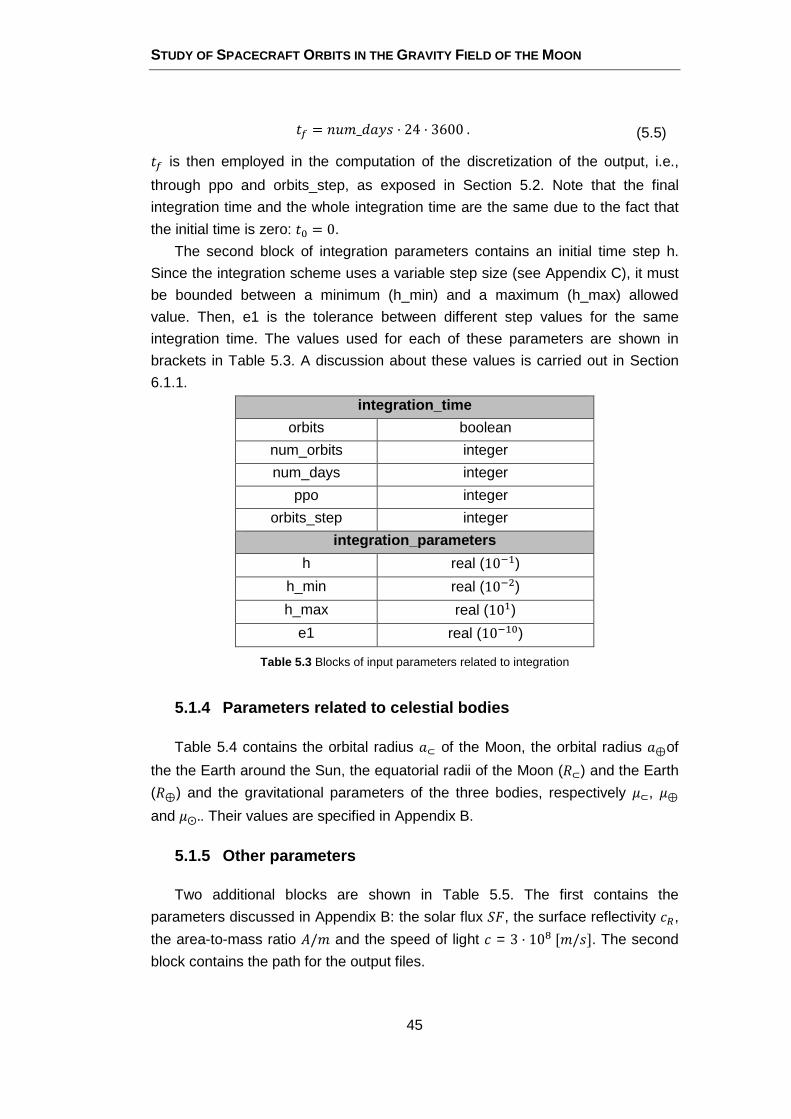
STUDY OF SPACECRAFT ORBITS IN THE GRAVITY FIELD OF THE MOON
45
�� = � �_'��F · 24 · 3600. (5.5)
�� is then employed in the computation of the discretization of the output, i.e.,
through ppo and orbits_step, as exposed in Section 5.2. Note that the final
integration time and the whole integration time are the same due to the fact that
the initial time is zero: �� = 0.
The second block of integration parameters contains an initial time step h.
Since the integration scheme uses a variable step size (see Appendix C), it must
be bounded between a minimum (h_min) and a maximum (h_max) allowed
value. Then, e1 is the tolerance between different step values for the same
integration time. The values used for each of these parameters are shown in
brackets in Table 5.3. A discussion about these values is carried out in Section
6.1.1.
integration_time
orbits boolean
num_orbits integer
num_days integer
ppo integer
orbits_step integer
integration_parameters
h real (10��)
h_min real (10�)
h_max real (10�)
e1 real (10���)
Table 5.3 Blocks of input parameters related to integration
5.1.4 Parameters related to celestial bodies
Table 5.4 contains the orbital radius �⊂ of the Moon, the orbital radius �⊕of
the the Earth around the Sun, the equatorial radii of the Moon (I⊂) and the Earth
(I⊕) and the gravitational parameters of the three bodies, respectively �⊂, �⊕
and �⨀.. Their values are specified in Appendix B.
5.1.5 Other parameters
Two additional blocks are shown in Table 5.5. The first contains the
parameters discussed in Appendix B: the solar flux +L, the surface reflectivity ��,
the area-to-mass ratio �/� and the speed of light � = 3 · 10 [�/F]. The second
block contains the path for the output files.
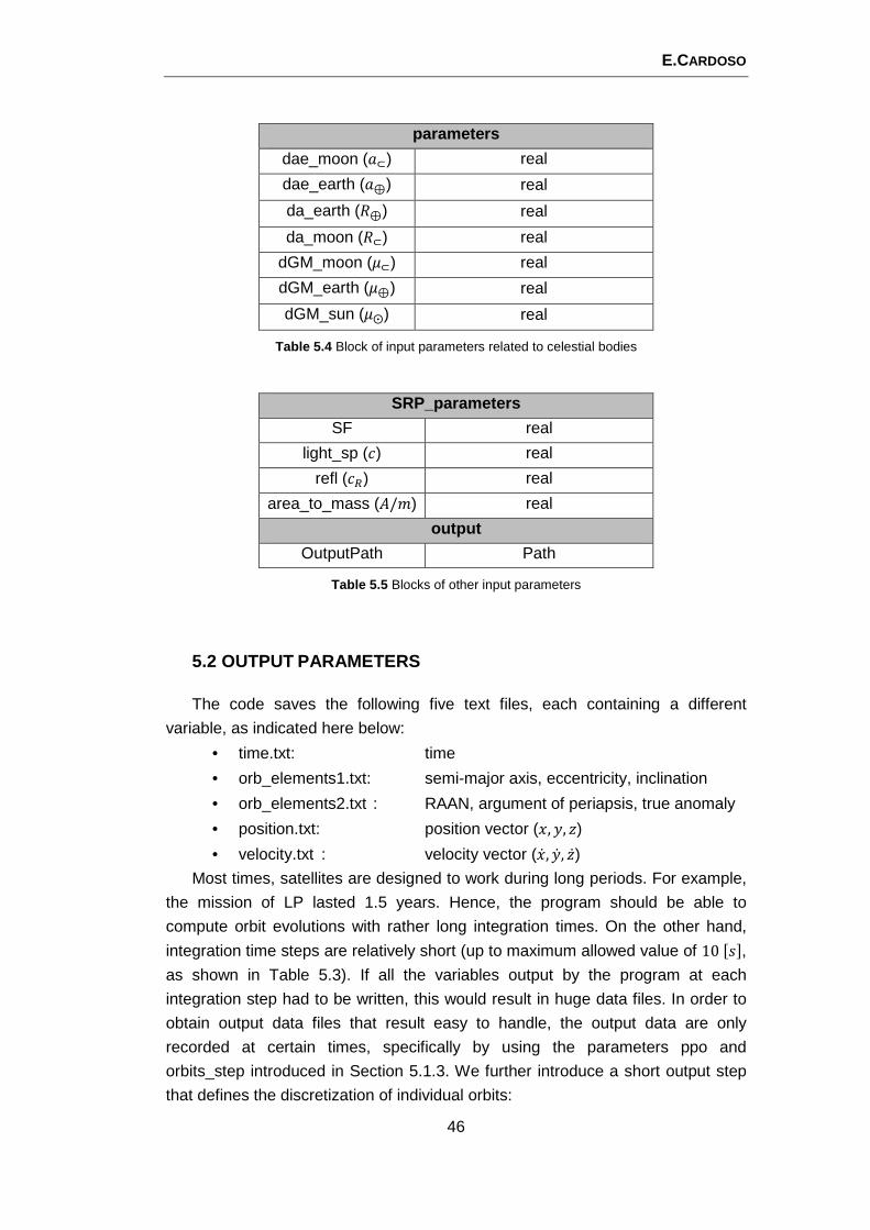
E.CARDOSO
46
parameters
dae_moon (�⊂) real
dae_earth (�⊕) real
da_earth (I⊕) real
da_moon (I⊂) real
dGM_moon (�⊂) real
dGM_earth (�⊕) real
dGM_sun (�⨀) real
Table 5.4 Block of input parameters related to celestial bodies
SRP_parameters
SF real
light_sp (�) real
refl (��) real
area_to_mass (�/�) real
output
OutputPath Path
Table 5.5 Blocks of other input parameters
5.2 OUTPUT PARAMETERS
The code saves the following five text files, each containing a different
variable, as indicated here below:
• time.txt: time
• orb_elements1.txt: semi-major axis, eccentricity, inclination
• orb_elements2.txt : RAAN, argument of periapsis, true anomaly
• position.txt: position vector (�,�, �)
• velocity.txt : velocity vector (�% ,�% , �%) Most times, satellites are designed to work during long periods. For example,
the mission of LP lasted 1.5 years. Hence, the program should be able to
compute orbit evolutions with rather long integration times. On the other hand,
integration time steps are relatively short (up to maximum allowed value of 102F3, as shown in Table 5.3). If all the variables output by the program at each
integration step had to be written, this would result in huge data files. In order to
obtain output data files that result easy to handle, the output data are only
recorded at certain times, specifically by using the parameters ppo and
orbits_step introduced in Section 5.1.3. We further introduce a short output step
that defines the discretization of individual orbits:
STUDY OF SPACECRAFT ORBITS IN THE GRAVITY FIELD OF THE MOON
47
FℎS$�_F��N = �NNS. (5.6)
It divides an orbit into ‘ppo’ equispaced time intervals and, helped by a counter,
determines when the output parameters have to be recorded.
Furthermore, the total integration time is divided into ‘orbits_step’ equidistant
time intervals:
US�_F��N = ��S$T��F_F��N. (5.7)
A counter determines when the output parameters have to be recorded. As an
example, if the orbital period is of 2,000[F], the whole integration time is
40,000[F], and ppo and orbits_step are 20 and 10, respectively, the short_step
and large_step are 100[F] and 4,000[F], respectively. The result is that for the
first period of 2,000[F] the output parameters are recorded every 100[F]. Then,
between 2,000[F] to 4,000[F] the output parameters are not recorded and are
saved between 4,000 and 6,000[F]. Hence, the parameters are written 20 times
per orbit in 10 equidistant different orbits.
5.3 CODE PERFORMANCE
Here we provide a general overview of the structure of the code. It consists of
15 source files written in Fortran90 language (see Table 5.7). Detailed
information is only provided for those functions which concern the general
comprehension of the program. The auxiliary functions and variables are not
explained.
The code consists of a main routine (Orbit_Integration) which calls specific
routines or functions for specialized computations. The input parameters are
introduced in ReadInputParameters subroutine. Then, allocation of matrices and
vectors is made based on the number of Stokes coefficients involved and
determined by gravity field input parameters (����, ��'�, ���� and ��'�). The
computation begins with the determination of the orbital elements of the satellite
or its position and velocity vectors, depending on which set of parameters has
been introduced by the user. The program needs both sets: the orbital elements
are used to compute the orbital period as in Eq. (5.3) and, consequently, the
short_step by means of Eq. (5.6). The state vector is needed as an input for the
numerical integration.
A while loop is employed to perform the numerical integration with the
following two stop conditions:
• End of integration: the time � exceeds ��,
E.CARDOSO
48
• Impact condition: the distance from the center of the Moon drops below I⊂ + ∆I, where ∆I represents the satellite’s minimum allowed altitude
over the surface. The highest point of the Moon has an altitude of
10.786[V�] 0 but a value of 7[V�] has been used in this study for polar
or near-polar orbit: Fig. 1.2 shows that only a small area in the far-side
exceeds 72V�3. For non-polar of orbits, ∆I has been set to 11[V�] to
avoid collisions with the topographical features.
Another condition that has been considered is when the altitude of the
satellite exceeds the value for which the Earth’s TB acceleration overcomes the
perturbations induced by the lunar gravity field, i.e. $ > I⊂ + 2,0002V�3 =3,738[V�]. In this case the execution does not stop, but a warning is given,
notifying the user that the orbit has gone beyond of what can be considered as
low-altitude.
Inside the while loop the routine RungeKutta78, which contains the numerical
integration: it computes the time and the state vector for the next step. This
function works as detailed in Appendix C using a total of 13 steps and
evaluations of the vector field (as an auxiliary routine: CalcVectorField). It
computes two different estimations of the next point. In any case, when the next
point is computed, the step h to be used in the next call of the routine is
predicted. The input parameters in this function are the current value of the
independent variable (��), the current value of the state vector (�-,�% -), the three
steps (h, h_max, h_min) and the tolerance (e1). The output are the next values of
the independent variable (����) and the state vector (�-�.,�% -�.), as well as the
time step to be used in the next call to this routine.
In CalcVectorField the six-components vector called field is filled in: �W�,W,W�� = ��% ,�% , �%�, �W/,W,W!� = (�& ,�& , �&), (5.8)
where W� (� = 1,… ,6) are the six components of the field vector. The objective of
CalcVectorField is to obtain the different components of the acceleration by
means of two auxiliary routines, PinesAccel which computes the acceleration due
to the lunar gravity field, and OtherAccel, which computes the remaining the
accelerations. The list below summarizes the tasks carried out by PinesAccel
(see Section 5.3.1)
• Determination of the spherical coordinates of the field point
• Computation and storage of various powers of �/$
• Computation of the trigonometric functions of the latitude "
• Computation of fully normalized HPs (fnHPs) and their derivatives
• Initialization and calculation of the lumped coefficients arrays
• If rotation of the tensors is required, then additional trigonometric
functions are computed for the longitude
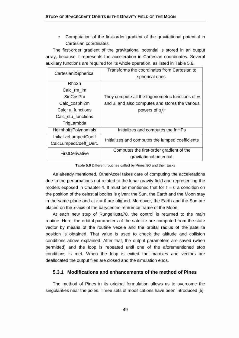
STUDY OF SPACECRAFT ORBITS IN THE GRAVITY FIELD OF THE MOON
49
• Computation of the first-order gradient of the gravitational potential in
Cartesian coordinates.
The first-order gradient of the gravitational potential is stored in an output
array, because it represents the acceleration in Cartesian coordinates. Several
auxiliary functions are required for its whole operation, as listed in Table 5.6.
Cartesian2Spherical Transforms the coordinates from Cartesian to
spherical ones.
Rho2n
Calc_rm_im
SinCosPhi
Calc_cosphi2m
Calc_u_functions
Calc_stu_functions
TrigLambda
They compute all the trigonometric functions of "
and , and also computes and stores the various
powers of �/$
HelmholtzPolynomials Initializes and computes the fnHPs
InitializeLumpedCoeff
CalcLumpedCoeff_Der1 Initializes and computes the lumped coefficients
FirstDerivative Computes the first-order gradient of the
gravitational potential.
Table 5.6 Different routines called by Pines.f90 and their tasks
As already mentioned, OtherAccel takes care of computing the accelerations
due to the perturbations not related to the lunar gravity field and representing the
models exposed in Chapter 4. It must be mentioned that for � = 0 a condition on
the position of the celestial bodies is given: the Sun, the Earth and the Moon stay
in the same plane and at � = 0 are aligned. Moreover, the Earth and the Sun are
placed on the �-axis of the barycentric reference frame of the Moon.
At each new step of RungeKutta78, the control is returned to the main
routine. Here, the orbital parameters of the satellite are computed from the state
vector by means of the routine vecele and the orbital radius of the satellite
position is obtained. That value is used to check the altitude and collision
conditions above explained. After that, the output parameters are saved (when
permitted) and the loop is repeated until one of the aforementioned stop
conditions is met. When the loop is exited the matrixes and vectors are
deallocated the output files are closed and the simulation ends.
5.3.1 Modifications and enhancements of the method of Pines
The method of Pines in its original formulation allows us to overcome the
singularities near the poles. Three sets of modifications have been introduced [5].
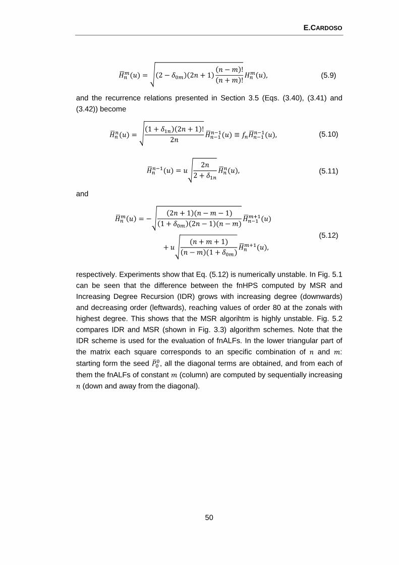
E.CARDOSO
50
�X��( ) = D�2 − �����2� + 1� �� −��!�� +��!���� �, (5.9)
and the recurrence relations presented in Section 3.5 (Eqs. (3.40), (3.41) and
(3.42)) become
�X��( ) = D�1 + �����2� + 1�!2� �X������( ) ≡ W��X������( ), (5.10)
�X����( ) = D 2�2 + ��� �X��( ), (5.11)
and
�X��� � = −D �2� + 1�(� −� − 1)�1 + �����2� − 1�(� −�)�X������( )+ D (� +� + 1)�� −��(1 + ���)�X����( ), (5.12)
respectively. Experiments show that Eq. (5.12) is numerically unstable. In Fig. 5.1
can be seen that the difference between the fnHPS computed by MSR and
Increasing Degree Recursion (IDR) grows with increasing degree (downwards)
and decreasing order (leftwards), reaching values of order 80 at the zonals with
highest degree. This shows that the MSR algorihtm is highly unstable. Fig. 5.2
compares IDR and MSR (shown in Fig. 3.3) algorithm schemes. Note that the
IDR scheme is used for the evaluation of fnALFs. In the lower triangular part of
the matrix each square corresponds to an specific combination of � and �:
starting form the seed �*��, all the diagonal terms are obtained, and from each of
them the fnALFs of constant � (column) are computed by sequentially increasing � (down and away from the diagonal).
STUDY OF SPACECRAFT ORBITS IN THE GRAVITY FIELD OF THE MOON
51
Fig. 5.1 Log10 of the difference between the fnHPs computed with the MSR algorithm and those resulting from adopting the IDR scheme
Fig. 5.2 Comparison between the IDR (left) and MSR (right) algorithm schemes
�X��� � = D�2� + 1�(2� − 1)
(� +�)(� −�) �X���� � �−D�2� + 1��� −� − 1��� +� − 1��2� − 3��� +���� −�� �X��� � �. (5.13)
The V(0 derivative of the HP of degree � and order � is the HP of degree � and
order �� + V�: '1��
�� �' 1 = ����1� �. (5.14)
E.CARDOSO
52
The only necessary derivative for this study is the first one, due to the fact that
the accelerations are the first derivatives of the potential and they will be
expressed, then, in terms of the first derivatives of the HP. It can be shown by
induction over the differentiation V, that its fully normalized form for the first
derivative is
'�X��� �' = D�2 − ������ −��(� +� + 1)
2�X����� �. (5.15)
5.3.2 Lumped coefficients synthesis of the geopoten tial and its
gradients
In this contribution, the Pines’ method has been rewritten in the lumped
coefficients form. It can be easily shown that
� = ? B��(�) cos� + 9�(�) sin� C�
���
cos� ", (5.16)
with ��(�) and 9�(�) given by
��(�) = ? !���̅��X���
���
,
9�(�) = ? !�+̅���X���
���
. (5.17)
As for the gradients, by application of the chain rule the differential operators of
the gravitational potential � with respect to the global coordinates �, �, � of � can
be written as a function of the differential operators with respect to $, F, � and : ((� = 1$ ((F + F 4 (($ − F$ ((F − �$ ((� − $ (( 5, ((� = 1$ ((� + � 4 (($ − F$ ((F − �$ ((� − $ (( 5, ((� = 1$ (( + 4 (($ − F$ ((F − �$ ((� − $ (( 5. (5.18)
By defining the operators
STUDY OF SPACECRAFT ORBITS IN THE GRAVITY FIELD OF THE MOON
53
Y� = 1$ ((F, Y = 1$ ((�, Y� = 1$ (( ,
Y/ = (($ − F$ ((F − �$ ((� − $ (( . (5.19)
Eqs. (5.18) can be rewritten more concisely as ((� = Y� + FY/, ((� = Y + �Y/, ((� = Y� + Y/.
(5.20)
Hence, differentiating the geopotential � of Eq. (5.16) with respect to global
Cartesian coordinates yields the components of the first-order gradient (the
notation of [4] has been used in representing the physical components of the
gradients) �� = �� + F�/, �2 = � + ��/, �3 = �� + �/, (5.21)
where the quantities �� (� = 1, 2, 3, 4) result from the application of the operators Y�, Y, Y� and Y/ to �, and their lumped coefficients expressions are given as
�� = ? �B��(�)���� + 9�(�)F���C�
���
cos���"
� = ? �B9�(�)���� − ��(�)F���C�
���
cos���"
�� = ? B��()�� + 9�()F�C�
���
cos� "
�/ = ? B��(�)�� + 9�(�)F�C�
���
cos� "
(5.22)
where the quantities ���� and F��� replace respectively the expressions
cos�� − A� and sin�� − A� . Moreover, must be mentioned that in working out
the expression of �/, the following relation has been used: (!�($ = −�� + 1� !���� ≡ −�� + 1� !�� . (5.23)
The expressions of the lumped coefficients needed for the first-gradient
calculations, besides those of Eq.(5.17), are
E.CARDOSO
54
��() = ? !��
���
��̅�'�X��/'
9�() = ? !��
���
+̅��'�X��/'
��(�) = ? !��
���
��̅�Y*��
9�(�) = ? !��
���
+̅��Y*��
(5.24)
and the auxiliary function Y*�� is defined as
Y*�� = (� +� + 1)�X�� + '�X��' . (5.25)
Note that differentiation of Eq. (5.21) with respect to �, �, � provides the second-
and third- order gravity gradients.
5.3.3 Summary of the routines involved in the progr am
Table 5.7 summarizes all the routines involved in the program and their main
task. Note that the routines complementary to PinesAccel are listed in Table 5.6
and not mentioned here.
Constants
Contains constants/definitions that are used in
several routines in order to not define them more
than once
greeks Defines the relations to pass from degrees to
radians and viceversa.
ReadInputParameters Reads the input information and writes the output
files
elevec/vecele Returns the position and velocity vectors from the
orbital elements and viceversa.
Orbit_Integration Main program
OtherAccel Determines the acceleration due to orbital
perturbations not related to lunar gravity field
PinesAccel Determines the accelerations due to the lunar
gravity field as developed in Chapter 3
RungeKutta78 Performs the numerical integration
ReadStokesCoeff Reads the Stokes Coefficients of the model
CalcVectorField Complementary to RungeKutta78
Table 5.7 The several routines involved in the program and the task they perform

STUDY OF SPACECRAFT ORBITS IN THE GRAVITY FIELD OF THE MOON
55
CHAPTER SIX.
SIMULATIONS
This chapter presents the simulations carried out with the code described in
the previous chapter. These simulations have been used to validate the
functionality of the code and to identify useful orbits for lunar missions.
This chapter begins with the definition of the value of some key parameters.
Then, the code validations are presented, followed by the illustration of some
selected orbits, with the most outstanding results detailed by means of tables and
figures. The final idea of the present study is to show the capabilities and the
applications of the developed software in a context of mission analysis. It must be
noted that some orbits are not low-altitude orbits: they have been included in the
sample in order to reproduce the results contained in the corresponding
references and decide if the hypotheses followed can give good results.
6.1 DEFINITION OF PARAMETERS
This sections deals with the definition of the code input parameters, such as
the integration time step and the integration tolerance and other parameters that
allow to discretize and adjust the output to the desired resolution while
maintaining an adequate numerical accuracy.
6.1.1 Integration steps
With an appropriate time step, the integration tolerance e1 determines the
precision of the results. However, choosing inadequate time steps can provide
huge errors even under a very restrictive tolerance. As a consequence, the
minimum and maximum allowed steps must be carefully determined. This
imposes an analysis to determine the time steps which better fulfill this
requirement. Fig. 6.1 shows the evolution of five orbital elements within a whole
orbit (note that the true anomaly evolution is comparable to the time evolution, so
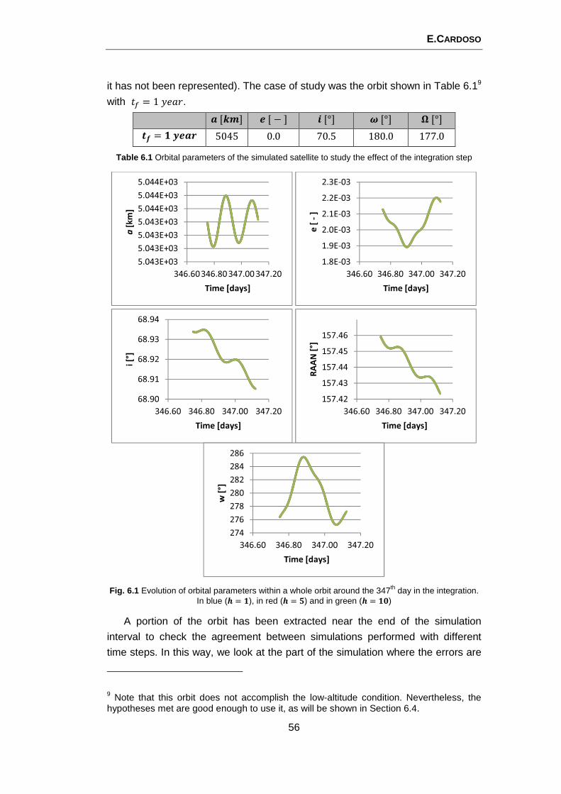
E.CARDOSO
56
it has not been represented). The case of study was the orbit shown in Table 6.19
with �� = 1���$.
Z[[\] ][−] ^[°] _[°] `[°] a4 = bc]Zd 5045 0.0 70.5 180.0 177.0
Table 6.1 Orbital parameters of the simulated satellite to study the effect of the integration step
Fig. 6.1 Evolution of orbital parameters within a whole orbit around the 347th day in the integration. In blue (� = �), in red (� = ) and in green (� = �)
A portion of the orbit has been extracted near the end of the simulation
interval to check the agreement between simulations performed with different
time steps. In this way, we look at the part of the simulation where the errors are
9 Note that this orbit does not accomplish the low-altitude condition. Nevertheless, the hypotheses met are good enough to use it, as will be shown in Section 6.4.
5.043E+03
5.043E+03
5.043E+03
5.043E+03
5.044E+03
5.044E+03
5.044E+03
346.60346.80347.00347.20
a [
km
]
Time [days]
1.8E-03
1.9E-03
2.0E-03
2.1E-03
2.2E-03
2.3E-03
346.60 346.80 347.00 347.20
e [
-]
Time [days]
68.90
68.91
68.92
68.93
68.94
346.60 346.80 347.00 347.20
i [°
]
Time [days]
157.42
157.43
157.44
157.45
157.46
346.60 346.80 347.00 347.20
RA
AN
[°]
Time [days]
274
276
278
280
282
284
286
346.60 346.80 347.00 347.20
w [
°]
Time [days]
STUDY OF SPACECRAFT ORBITS IN THE GRAVITY FIELD OF THE MOON
57
amplified. Fig. 6.1 shows that the different integration steps do not modify
appreciably the orbital evolution. On the other hand, Table 6.2 shows that the
different values of h produce large differences in the simulation elapsed time. The
comparison is in favor of ℎ = 10.
Integration time step Simulation elapsed time e = b 18014�5� e = f 3037�58� e = bg 1049�11�
Table 6.2 Simulation elapsed time versus integration time step
6.1.2 Tolerance
The tolerance e1 determines the precision of the results in the integration, but
it also influences the duration of the simulations. Hence, a trade-off has to be
made between the simulation time and the precision of the results. Taking into
account that the order of magnitude of the perturbing accelerations ranges
between 10−3 and 10−8 [�/F], the minimum time step has been set at 10−2,
and the tolerance at 10−10. An order of magnitude estimation:
�$$S$2�/F3~����ℎ����1 =10� 10�
10���= 1[�/F], (6.1)
which corresponds to a reasonable spatial error, considering that a satellite 100
meters above the lunar surface would be moving at more than 1600[�/F]. 6.1.3 Output temporal resolution
An external script (see Annex B) that runs under MATLAB takes care of
plotting the several orbits obtained with the code. The output temporal resolution
is the resolution shown in the graphics obtained. It can be modified by means of
the parameters ppo and orbits_step defined in Section 5.1.3. The latter is defines
how close the different output orbits are and it depends of the duration of the
integration time, which can vary from few weeks to several years depending on
the mission. These aspects make it more difficult to a priori choose the most
appropriate value for orbits_step. The parameter ppo defines how smooth the
orbits look like: the point is to have a ppo large enough to obtain smooth orbits,
but small enough to avoid saving too much data. Fig. 6.2 shows that 40 is a good
compromise.
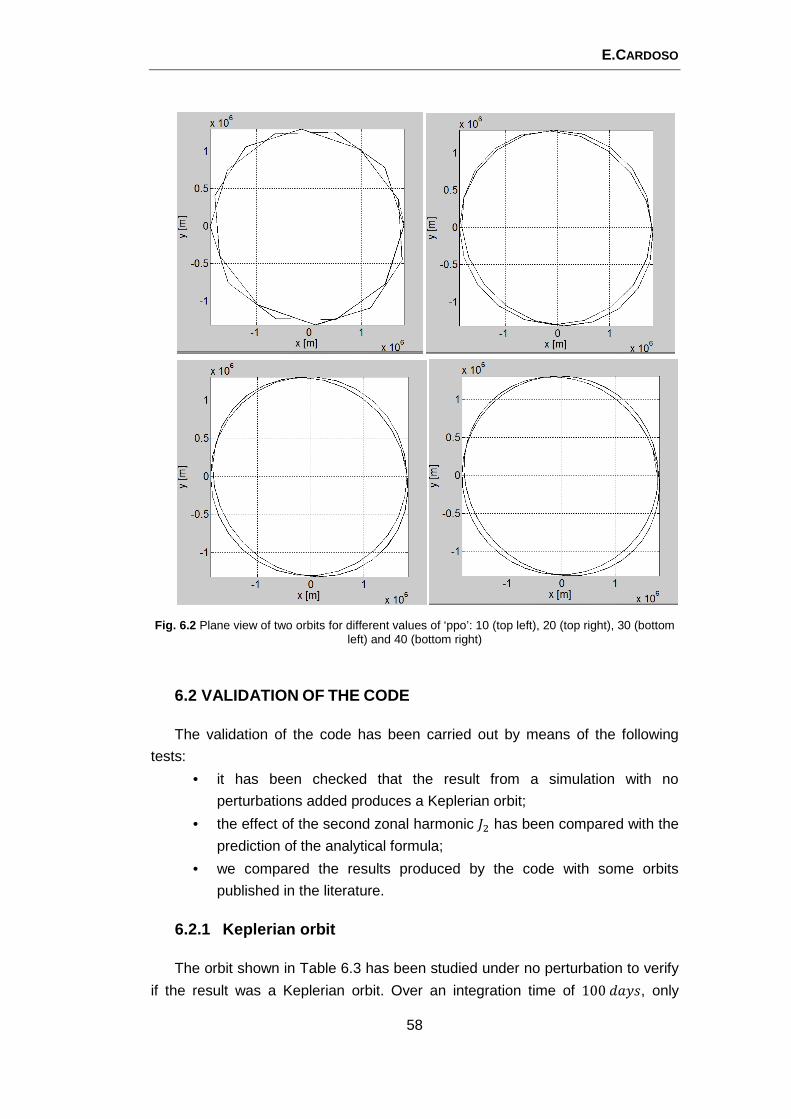
E.CARDOSO
58
Fig. 6.2 Plane view of two orbits for different values of ‘ppo’: 10 (top left), 20 (top right), 30 (bottom left) and 40 (bottom right)
6.2 VALIDATION OF THE CODE
The validation of the code has been carried out by means of the following
tests:
• it has been checked that the result from a simulation with no
perturbations added produces a Keplerian orbit;
• the effect of the second zonal harmonic � has been compared with the
prediction of the analytical formula;
• we compared the results produced by the code with some orbits
published in the literature.
6.2.1 Keplerian orbit
The orbit shown in Table 6.3 has been studied under no perturbation to verify
if the result was a Keplerian orbit. Over an integration time of 100'��F, only
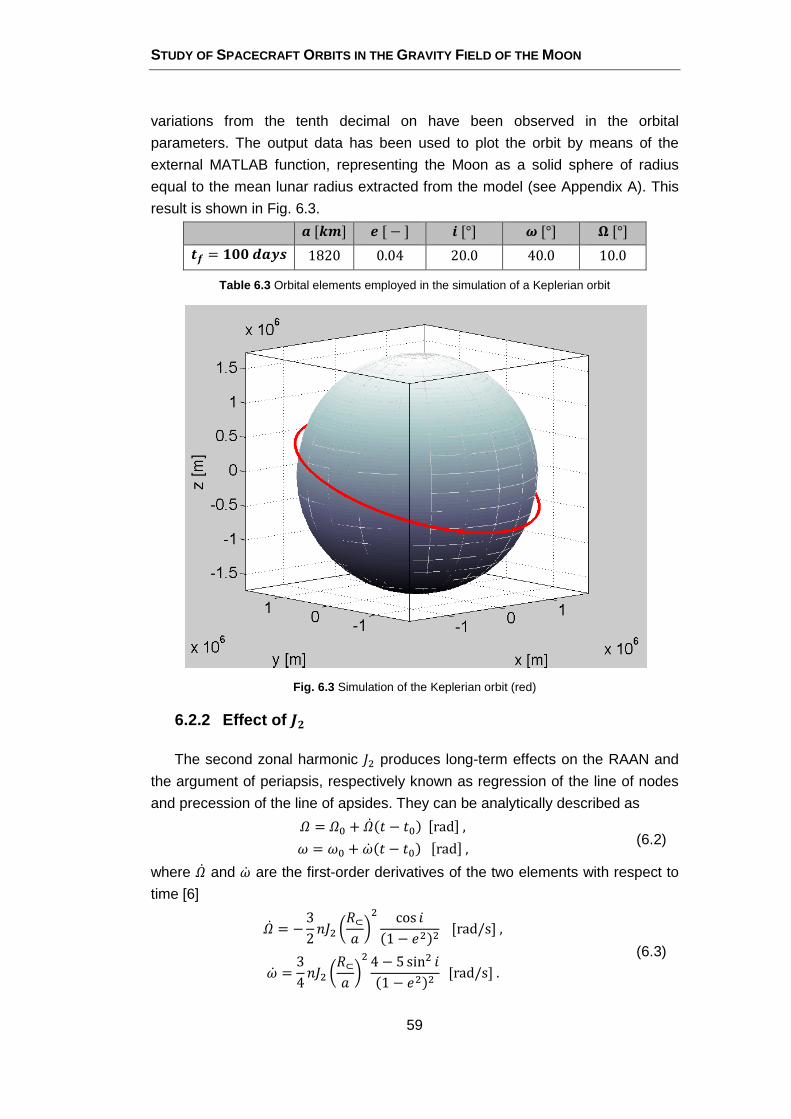
STUDY OF SPACECRAFT ORBITS IN THE GRAVITY FIELD OF THE MOON
59
variations from the tenth decimal on have been observed in the orbital
parameters. The output data has been used to plot the orbit by means of the
external MATLAB function, representing the Moon as a solid sphere of radius
equal to the mean lunar radius extracted from the model (see Appendix A). This
result is shown in Fig. 6.3.
Z[[\] ][−] ^[°] _[°] `[°] a4 = bgghZci 1820 0.04 20.0 40.0 10.0
Table 6.3 Orbital elements employed in the simulation of a Keplerian orbit
Fig. 6.3 Simulation of the Keplerian orbit (red)
6.2.2 Effect of ��
The second zonal harmonic � produces long-term effects on the RAAN and
the argument of periapsis, respectively known as regression of the line of nodes
and precession of the line of apsides. They can be analytically described as R = R� + R% �� − ���2rad3, # = #� +#% �� − ���2rad3, (6.2)
where R% and #% are the first-order derivatives of the two elements with respect to
time [6]
R% = −3
2�� 4I⊂� 5 cos ��1 − �� [rad/s],
#% = 3
4�� 4I⊂� 5 4 − 5 sin ��1 − �� [rad/s]. (6.3)
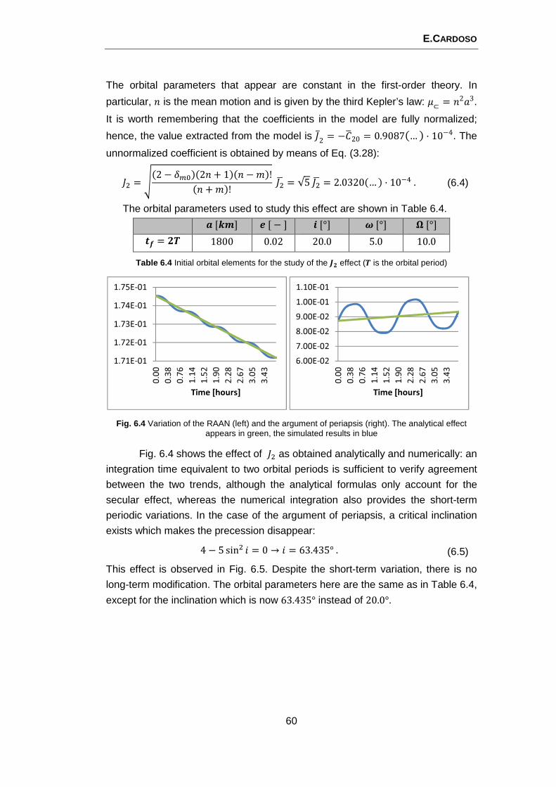
E.CARDOSO
60
The orbital parameters that appear are constant in the first-order theory. In
particular, � is the mean motion and is given by the third Kepler’s law: �⊂= �2�3.
It is worth remembering that the coefficients in the model are fully normalized;
hence, the value extracted from the model is �̅2= −��20 = 0.9087�… � · 10−4. The
unnormalized coefficient is obtained by means of Eq. (3.28):
� = D�2 − �����2�+ 1��� −��!�� +��! �X = √5�X = 2.0320�… � · 10�/. (6.4)
The orbital parameters used to study this effect are shown in Table 6.4.
Z[[\] ][−] ^[°] _[°] `[°] a4 = kl 1800 0.02 20.0 5.0 10.0
Table 6.4 Initial orbital elements for the study of the �� effect (� is the orbital period)
Fig. 6.4 Variation of the RAAN (left) and the argument of periapsis (right). The analytical effect appears in green, the simulated results in blue
Fig. 6.4 shows the effect of � as obtained analytically and numerically: an
integration time equivalent to two orbital periods is sufficient to verify agreement
between the two trends, although the analytical formulas only account for the
secular effect, whereas the numerical integration also provides the short-term
periodic variations. In the case of the argument of periapsis, a critical inclination
exists which makes the precession disappear:
4 − 5 sin � = 0 → � = 63.435°. (6.5)
This effect is observed in Fig. 6.5. Despite the short-term variation, there is no
long-term modification. The orbital parameters here are the same as in Table 6.4,
except for the inclination which is now 63.435° instead of 20.0°.
1.71E-01
1.72E-01
1.73E-01
1.74E-01
1.75E-01
0.00
0.38
0.76
1.14
1.52
1.90
2.28
2.67
3.05
3.43
Time [hours]
6.00E-02
7.00E-02
8.00E-02
9.00E-02
1.00E-01
1.10E-01
0.00
0.38
0.76
1.14
1.52
1.90
2.28
2.67
3.05
3.43
Time [hours]
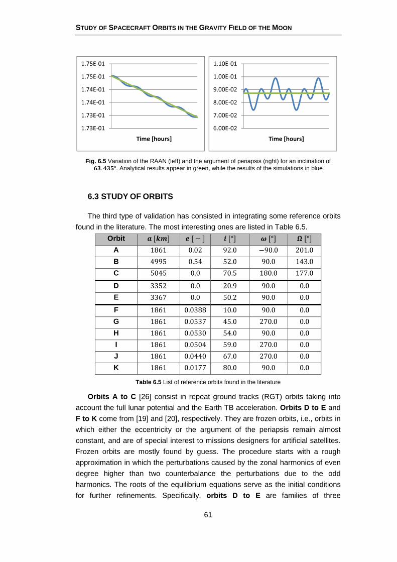
STUDY OF SPACECRAFT ORBITS IN THE GRAVITY FIELD OF THE MOON
61
Fig. 6.5 Variation of the RAAN (left) and the argument of periapsis (right) for an inclination of �.��°. Analytical results appear in green, while the results of the simulations in blue
6.3 STUDY OF ORBITS
The third type of validation has consisted in integrating some reference orbits
found in the literature. The most interesting ones are listed in Table 6.5.
Orbit Z[[\] ][−] ^[°] _[°] `[°] A 1861 0.02 92.0 −90.0 201.0
B 4995 0.54 52.0 90.0 143.0
C 5045 0.0 70.5 180.0 177.0
D 3352 0.0 20.9 90.0 0.0
E 3367 0.0 50.2 90.0 0.0
F 1861 0.0388 10.0 90.0 0.0
G 1861 0.0537 45.0 270.0 0.0
H 1861 0.0530 54.0 90.0 0.0
I 1861 0.0504 59.0 270.0 0.0
J 1861 0.0440 67.0 270.0 0.0
K 1861 0.0177 80.0 90.0 0.0
Table 6.5 List of reference orbits found in the literature
Orbits A to C [26] consist in repeat ground tracks (RGT) orbits taking into
account the full lunar potential and the Earth TB acceleration. Orbits D to E and
F to K come from [19] and [20], respectively. They are frozen orbits, i.e., orbits in
which either the eccentricity or the argument of the periapsis remain almost
constant, and are of special interest to missions designers for artificial satellites.
Frozen orbits are mostly found by guess. The procedure starts with a rough
approximation in which the perturbations caused by the zonal harmonics of even
degree higher than two counterbalance the perturbations due to the odd
harmonics. The roots of the equilibrium equations serve as the initial conditions
for further refinements. Specifically, orbits D to E are families of three
1.73E-01
1.73E-01
1.74E-01
1.74E-01
1.75E-01
1.75E-01
Time [hours]
6.00E-02
7.00E-02
8.00E-02
9.00E-02
1.00E-01
1.10E-01
Time [hours]
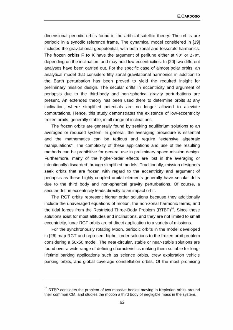
E.CARDOSO
62
dimensional periodic orbits found in the artificial satellite theory. The orbits are
periodic in a synodic reference frame. The dynamical model considered in [19]
includes the gravitational geopotential, with both zonal and tesserals harmonics.
The frozen orbits F to K have the argument of perilune either at 90° or 270°,
depending on the inclination, and may hold low eccentricities. In [20] two different
analyses have been carried out. For the specific case of almost polar orbits, an
analytical model that considers fifty zonal gravitational harmonics in addition to
the Earth perturbation has been proved to yield the required insight for
preliminary mission design. The secular drifts in eccentricity and argument of
periapsis due to the third-body and non-spherical gravity perturbations are
present. An extended theory has been used there to determine orbits at any
inclination, where simplified potentials are no longer allowed to alleviate
computations. Hence, this study demonstrates the existence of low-eccentricity
frozen orbits, generally stable, in all range of inclinations.
The frozen orbits are generally found by seeking equilibrium solutions to an
averaged or reduced system. In general, the averaging procedure is essential
and the mathematics can be tedious and require “extensive algebraic
manipulations”. The complexity of these applications and use of the resulting
methods can be prohibitive for general use in preliminary space mission design.
Furthermore, many of the higher-order effects are lost in the averaging or
intentionally discarded through simplified models. Traditionally, mission designers
seek orbits that are frozen with regard to the eccentricity and argument of
periapsis as these highly coupled orbital elements generally have secular drifts
due to the third body and non-spherical gravity perturbations. Of course, a
secular drift in eccentricity leads directly to an impact orbit.
The RGT orbits represent higher order solutions because they additionally
include the unaveraged equations of motion, the non-zonal harmonic terms, and
the tidal forces from the Restricted Three-Body Problem (RTBP)10. Since these
solutions exist for most altitudes and inclinations, and they are not limited to small
eccentricity, lunar RGT orbits are of direct application to a variety of missions.
For the synchronously rotating Moon, periodic orbits in the model developed
in [26] map RGT and represent higher-order solutions to the frozen orbit problem
considering a 50x50 model. The near-circular, stable or near-stable solutions are
found over a wide range of defining characteristics making them suitable for long-
lifetime parking applications such as science orbits, crew exploration vehicle
parking orbits, and global coverage constellation orbits. Of the most promising
10 RTBP considers the problem of two massive bodies moving in Keplerian orbits around their common CM, and studies the motion a third body of negligible mass in the system.

STUDY OF SPACECRAFT ORBITS IN THE GRAVITY FIELD OF THE MOON
63
results are the low-altitude families of near-circular, inclined orbits that maintain
long-term stability despite the highly non-spherical lunar gravity (e.g. Orbit A).
The aimed missions are likely to require extended stays and global
communication coverage. Therein lays the challenge to find long-lifetime orbits in
the vicinity of the Moon. Hence, RGT lunar orbits are useful for many different
missions including mapping missions when the repeat cycle is long enough. It
can be shown that periodic orbits of simplified models generally remain as RGT
orbits in the full ephemeris models. However, this does not apply to the lumpy
Moon where it has been shown that lower order zonals, particularly �5, notably
affect the long-term behavior of low altitude orbits. For simple resonances, or
RGT cycles, the near-polar, near-circular solutions of the perturbed three-body
problem are found to be linearly stable for altitudes less than ~1200[V�]. At the
higher altitudes, the families evolve into stable moderately-inclined eccentric
orbits. The stable and near-stable families of solutions are shown to exist for a full
range of average inclinations and altitudes making them suitable for long-lifetime
parking applications such as science orbits, crew exploration vehicle parking
orbits, and global coverage constellation orbits ([10], [11] and [26]).
6.4 SIMULATIONS
Here we describe the simulations carried out on the above orbits and some
others. Note that some discrepancies with respect to the literature may appear:
an orbit that is considered frozen within a certain model might impact the lunar
surface if considered under a different set of perturbations or with an improved
definition of the lunar gravity field.
The objective of the simulation is to realize two alternative orbit design
strategies: optimization with respect to fuel consumption or taking advantage
from the natural evolution resulting from the orbital perturbations.
Besides the orbits listed in Section 6.3, some polar orbits have been also
studied. Hence, the current section has been divided into three parts: the first
deals with the frozen orbits D to K of Table 6.5, the second is about the RGT
lunar orbits (A to C in Table 6.5), and a third section is dedicated to the study of
polar orbits. In each specific subsection the benefits of the most outstanding orbit
is discussed in the context of future lunar missions.
6.4.1 Frozen orbits
All the low-altitude lunar frozen orbits F to K from Table 6.5 have semi-major
axis � = 1861[V�], i.e., that they all have an orbital period � = 7204[F].
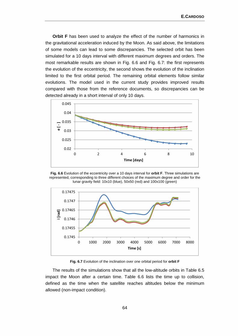
E.CARDOSO
64
Orbit F has been used to analyze the effect of the number of harmonics in
the gravitational acceleration induced by the Moon. As said above, the limitations
of some models can lead to some discrepancies. The selected orbit has been
simulated for a 10 days interval with different maximum degrees and orders. The
most remarkable results are shown in Fig. 6.6 and Fig. 6.7: the first represents
the evolution of the eccentricity, the second shows the evolution of the inclination
limited to the first orbital period. The remaining orbital elements follow similar
evolutions. The model used in the current study provides improved results
compared with those from the reference documents, so discrepancies can be
detected already in a short interval of only 10 days.
Fig. 6.6 Evolution of the eccentricity over a 10 days interval for orbit F. Three simulations are represented, corresponding to three different choices of the maximum degree and order for the
lunar gravity field: 10x10 (blue), 50x50 (red) and 100x100 (green)
Fig. 6.7 Evolution of the inclination over one orbital period for orbit F
The results of the simulations show that all the low-altitude orbits in Table 6.5
impact the Moon after a certain time. Table 6.6 lists the time up to collision,
defined as the time when the satellite reaches altitudes below the minimum
allowed (non-impact condition).
0.02
0.025
0.03
0.035
0.04
0.045
0 2 4 6 8 10
e [
-]
Time [days]
0.1745
0.17455
0.1746
0.17465
0.1747
0.17475
0 1000 2000 3000 4000 5000 6000 7000 8000
i [r
ad
]
Time [s]
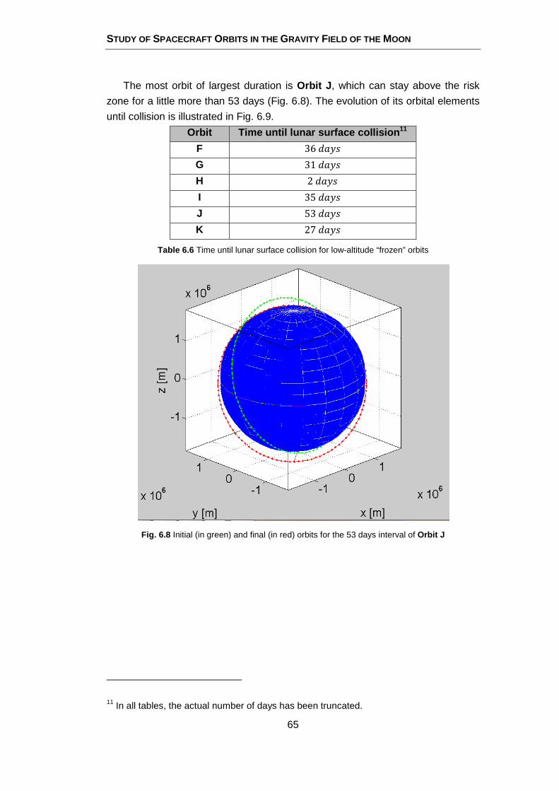
STUDY OF SPACECRAFT ORBITS IN THE GRAVITY FIELD OF THE MOON
65
The most orbit of largest duration is Orbit J, which can stay above the risk
zone for a little more than 53 days (Fig. 6.8). The evolution of its orbital elements
until collision is illustrated in Fig. 6.9.
Orbit Time until lunar surface collision11
F 36'��F
G 31'��F H 2'��F
I 35'��F J 53'��F K 27'��F
Table 6.6 Time until lunar surface collision for low-altitude “frozen” orbits
Fig. 6.8 Initial (in green) and final (in red) orbits for the 53 days interval of Orbit J
11 In all tables, the actual number of days has been truncated.
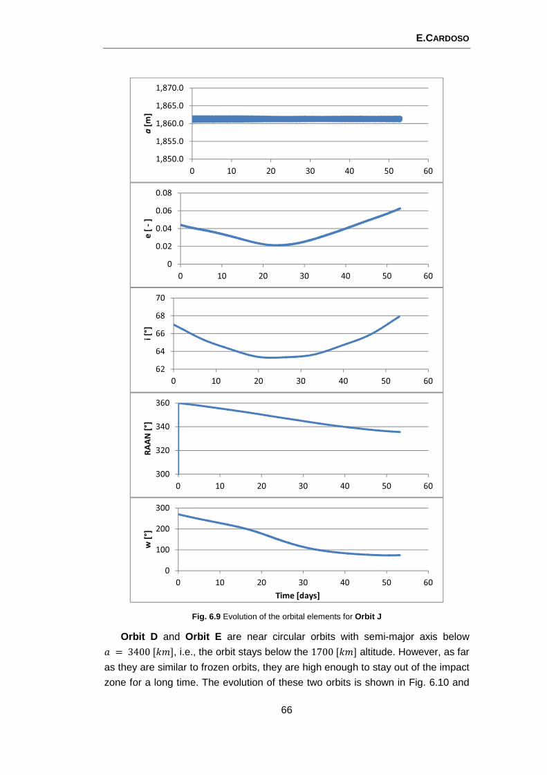
E.CARDOSO
66
Fig. 6.9 Evolution of the orbital elements for Orbit J
Orbit D and Orbit E are near circular orbits with semi-major axis below � = 3400[V�], i.e., the orbit stays below the 1700[V�] altitude. However, as far
as they are similar to frozen orbits, they are high enough to stay out of the impact
zone for a long time. The evolution of these two orbits is shown in Fig. 6.10 and
1,850.0
1,855.0
1,860.0
1,865.0
1,870.0
0 10 20 30 40 50 60
a[m
]
0
0.02
0.04
0.06
0.08
0 10 20 30 40 50 60
e [
-]
62
64
66
68
70
0 10 20 30 40 50 60
i [°
]
300
320
340
360
0 10 20 30 40 50 60
RA
AN
[°]
0
100
200
300
0 10 20 30 40 50 60
w [
°]
Time [days]
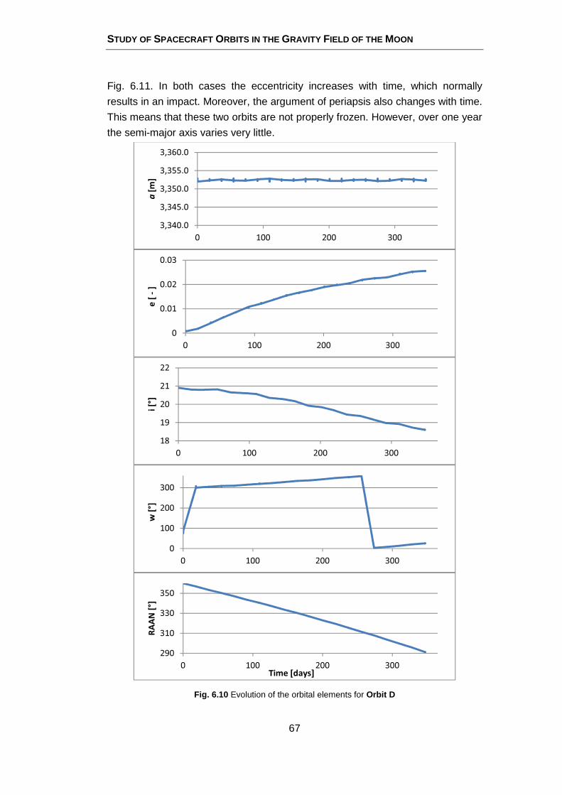
STUDY OF SPACECRAFT ORBITS IN THE GRAVITY FIELD OF THE MOON
67
Fig. 6.11. In both cases the eccentricity increases with time, which normally
results in an impact. Moreover, the argument of periapsis also changes with time.
This means that these two orbits are not properly frozen. However, over one year
the semi-major axis varies very little.
Fig. 6.10 Evolution of the orbital elements for Orbit D
3,340.0
3,345.0
3,350.0
3,355.0
3,360.0
0 100 200 300
a[m
]
0
0.01
0.02
0.03
0 100 200 300
e [
-]
18
19
20
21
22
0 100 200 300
i [°
]
0
100
200
300
0 100 200 300
w [
°]
290
310
330
350
0 100 200 300
RA
AN
[°]
Time [days]
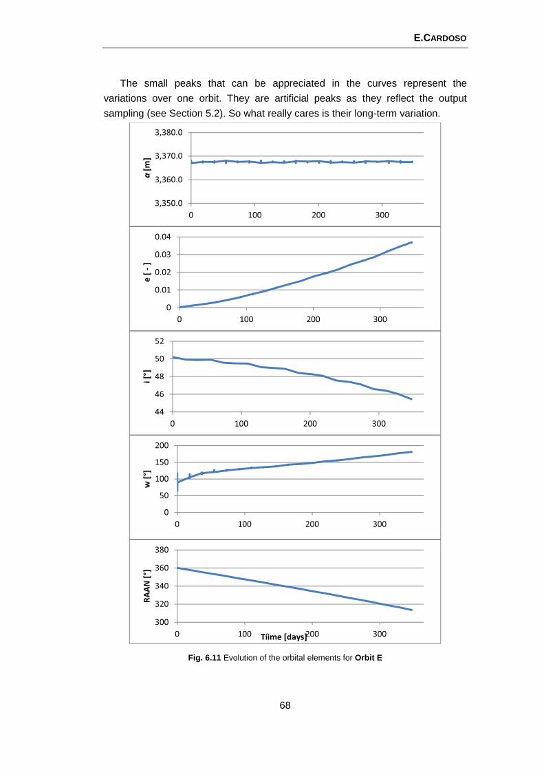
E.CARDOSO
68
The small peaks that can be appreciated in the curves represent the
variations over one orbit. They are artificial peaks as they reflect the output
sampling (see Section 5.2). So what really cares is their long-term variation.
Fig. 6.11 Evolution of the orbital elements for Orbit E
3,350.0
3,360.0
3,370.0
3,380.0
0 100 200 300
a[m
]
0
0.01
0.02
0.03
0.04
0 100 200 300
e [
-]
44
46
48
50
52
0 100 200 300
i [°
]
0
50
100
150
200
0 100 200 300
w [
°]
300
320
340
360
380
0 100 200 300
RA
AN
[°]
Tíime [days]
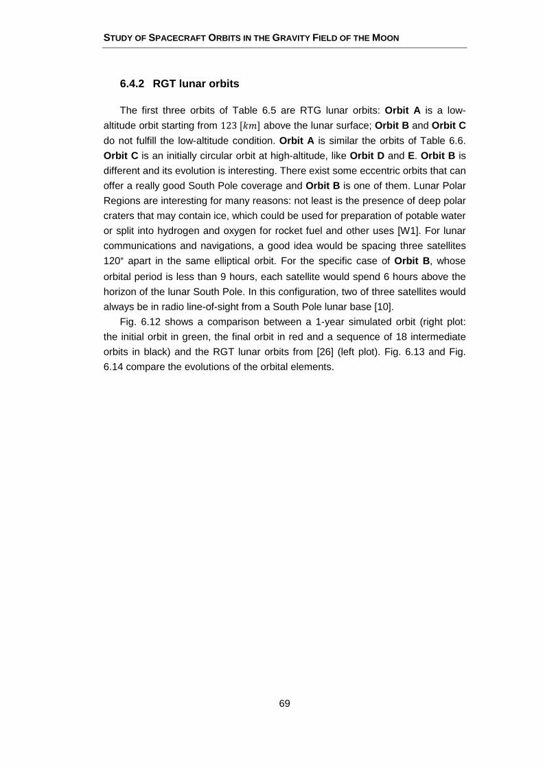
STUDY OF SPACECRAFT ORBITS IN THE GRAVITY FIELD OF THE MOON
69
6.4.2 RGT lunar orbits
The first three orbits of Table 6.5 are RTG lunar orbits: Orbit A is a low-
altitude orbit starting from 123[V�] above the lunar surface; Orbit B and Orbit C
do not fulfill the low-altitude condition. Orbit A is similar the orbits of Table 6.6.
Orbit C is an initially circular orbit at high-altitude, like Orbit D and E. Orbit B is
different and its evolution is interesting. There exist some eccentric orbits that can
offer a really good South Pole coverage and Orbit B is one of them. Lunar Polar
Regions are interesting for many reasons: not least is the presence of deep polar
craters that may contain ice, which could be used for preparation of potable water
or split into hydrogen and oxygen for rocket fuel and other uses [W1]. For lunar
communications and navigations, a good idea would be spacing three satellites
120° apart in the same elliptical orbit. For the specific case of Orbit B, whose
orbital period is less than 9 hours, each satellite would spend 6 hours above the
horizon of the lunar South Pole. In this configuration, two of three satellites would
always be in radio line-of-sight from a South Pole lunar base [10].
Fig. 6.12 shows a comparison between a 1-year simulated orbit (right plot:
the initial orbit in green, the final orbit in red and a sequence of 18 intermediate
orbits in black) and the RGT lunar orbits from [26] (left plot). Fig. 6.13 and Fig.
6.14 compare the evolutions of the orbital elements.
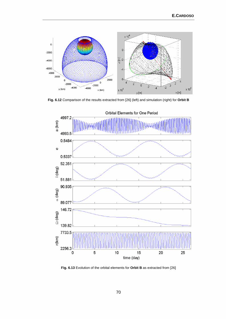
E.CARDOSO
70
Fig. 6.12 Comparison of the results extracted from [26] (left) and simulation (right) for Orbit B
Fig. 6.13 Evolution of the orbital elements for Orbit B as extracted from [26]
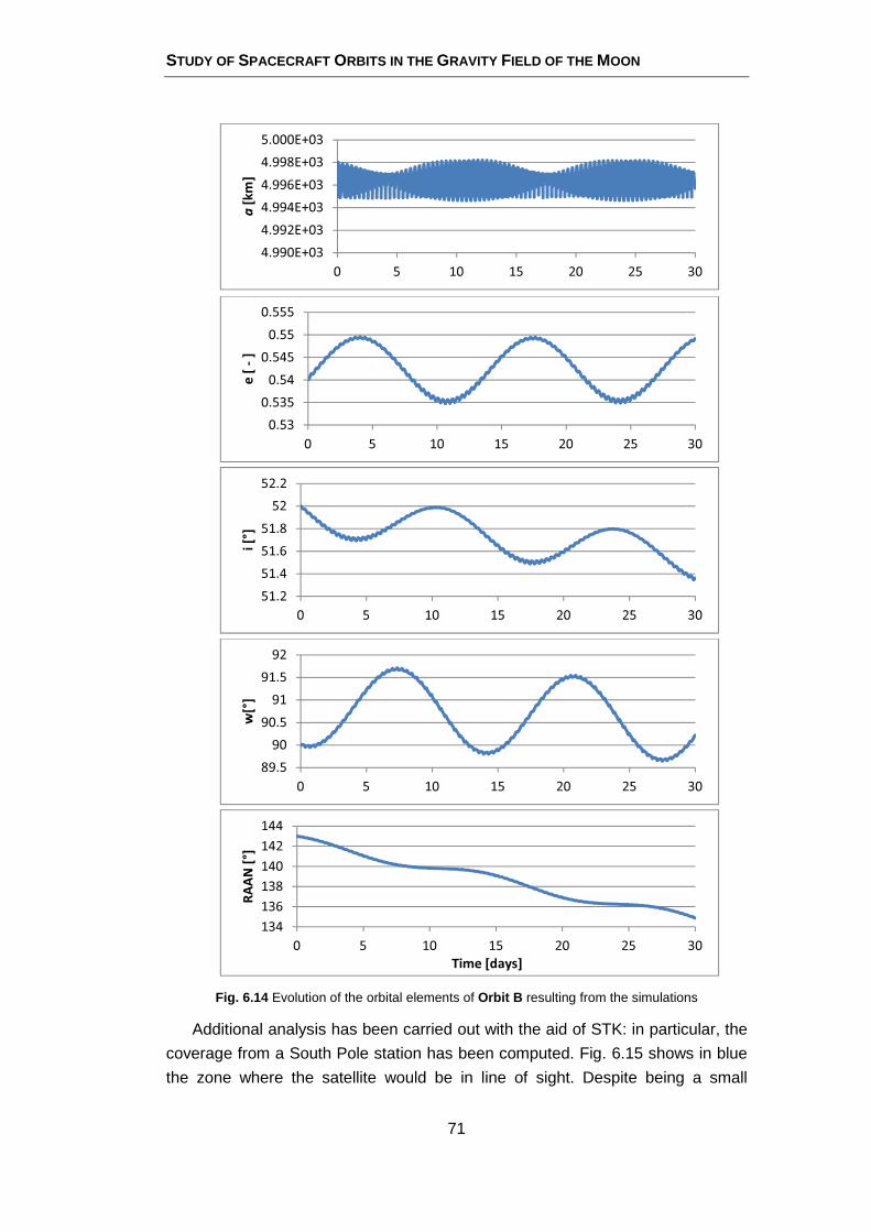
STUDY OF SPACECRAFT ORBITS IN THE GRAVITY FIELD OF THE MOON
71
Fig. 6.14 Evolution of the orbital elements of Orbit B resulting from the simulations
Additional analysis has been carried out with the aid of STK: in particular, the
coverage from a South Pole station has been computed. Fig. 6.15 shows in blue
the zone where the satellite would be in line of sight. Despite being a small
4.990E+03
4.992E+03
4.994E+03
4.996E+03
4.998E+03
5.000E+03
0 5 10 15 20 25 30
a[k
m]
0.53
0.535
0.54
0.545
0.55
0.555
0 5 10 15 20 25 30
e [
-]
51.2
51.4
51.6
51.8
52
52.2
0 5 10 15 20 25 30
i [°
]
89.5
90
90.5
91
91.5
92
0 5 10 15 20 25 30
w[°
]
134
136
138
140
142
144
0 5 10 15 20 25 30
RA
AN
[°]
Time [days]
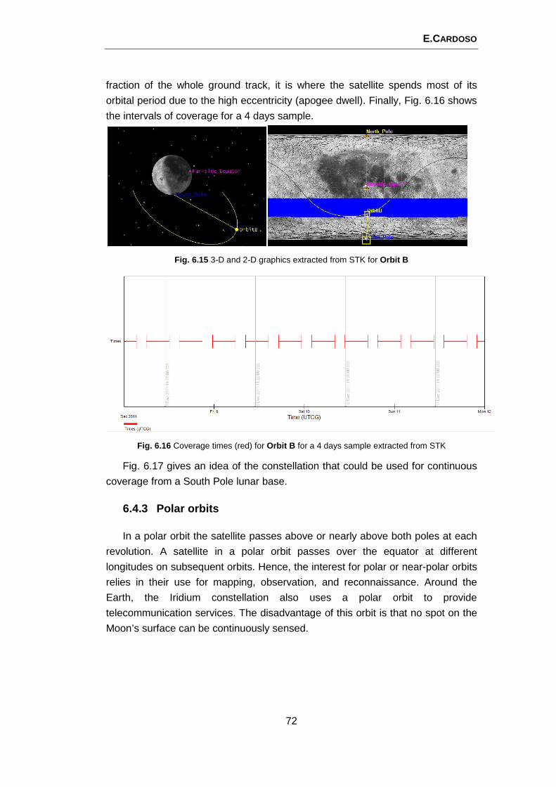
E.CARDOSO
72
fraction of the whole ground track, it is where the satellite spends most of its
orbital period due to the high eccentricity (apogee dwell). Finally, Fig. 6.16 shows
the intervals of coverage for a 4 days sample.
Fig. 6.15 3-D and 2-D graphics extracted from STK for Orbit B
Fig. 6.16 Coverage times (red) for Orbit B for a 4 days sample extracted from STK
Fig. 6.17 gives an idea of the constellation that could be used for continuous
coverage from a South Pole lunar base.
6.4.3 Polar orbits
In a polar orbit the satellite passes above or nearly above both poles at each
revolution. A satellite in a polar orbit passes over the equator at different
longitudes on subsequent orbits. Hence, the interest for polar or near-polar orbits
relies in their use for mapping, observation, and reconnaissance. Around the
Earth, the Iridium constellation also uses a polar orbit to provide
telecommunication services. The disadvantage of this orbit is that no spot on the
Moon’s surface can be continuously sensed.
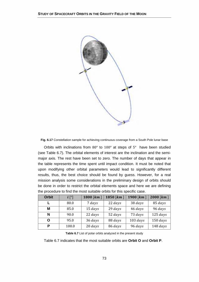
STUDY OF SPACECRAFT ORBITS IN THE GRAVITY FIELD OF THE MOON
73
Fig. 6.17 Constellation sample for achieving continuous coverage from a South Pole lunar base
Orbits with inclinations from 80° to 100° at steps of 5° have been studied
(see Table 6.7). The orbital elements of interest are the inclination and the semi-
major axis. The rest have been set to zero. The number of days that appear in
the table represents the time spent until impact condition. It must be noted that
upon modifying other orbital parameters would lead to significantly different
results, thus, the best choice should be found by guess. However, for a real
mission analysis some considerations in the preliminary design of orbits should
be done in order to restrict the orbital elements space and here we are defining
the procedure to find the most suitable orbits for this specific case.
Orbit ^[°] bmgg[[\] bmfg[[\] bngg[[\] kggg[[\] L 80.0 7'��F 22'��F 38'��F 85'��F M 85.0 15'��F 29'��F 46'��F 96'��F N 90.0 22'��F 52'��F 73'��F 125'��F O 95.0 36'��F 88'��F 103'��F 150'��F P 100.0 20'��F 86'��F 96'��F 148'��F
Table 6.7 List of polar orbits analyzed in the present study
Table 6.7 indicates that the most suitable orbits are Orbit O and Orbit P.
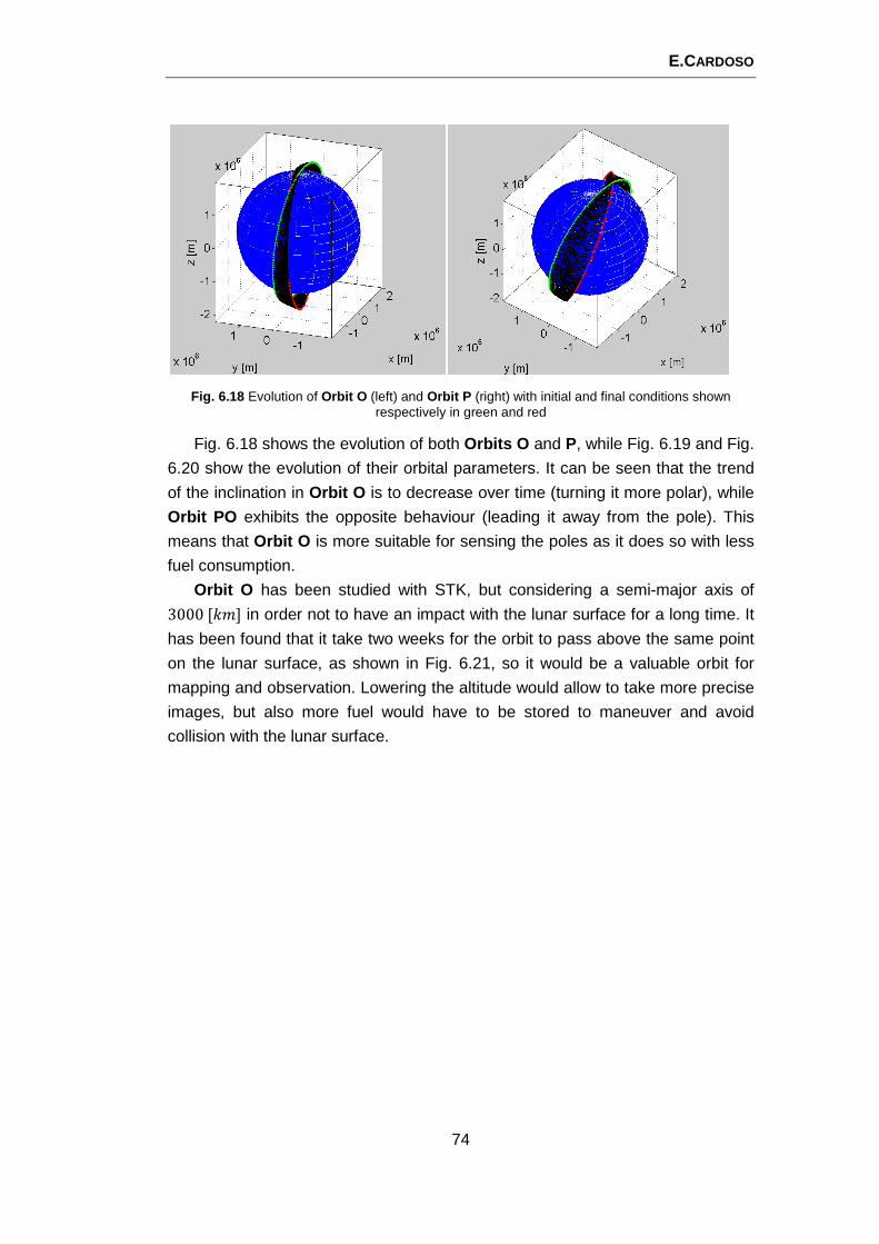
E.CARDOSO
74
Fig. 6.18 Evolution of Orbit O (left) and Orbit P (right) with initial and final conditions shown respectively in green and red
Fig. 6.18 shows the evolution of both Orbits O and P, while Fig. 6.19 and Fig.
6.20 show the evolution of their orbital parameters. It can be seen that the trend
of the inclination in Orbit O is to decrease over time (turning it more polar), while
Orbit PO exhibits the opposite behaviour (leading it away from the pole). This
means that Orbit O is more suitable for sensing the poles as it does so with less
fuel consumption.
Orbit O has been studied with STK, but considering a semi-major axis of
3000[V�] in order not to have an impact with the lunar surface for a long time. It
has been found that it take two weeks for the orbit to pass above the same point
on the lunar surface, as shown in Fig. 6.21, so it would be a valuable orbit for
mapping and observation. Lowering the altitude would allow to take more precise
images, but also more fuel would have to be stored to maneuver and avoid
collision with the lunar surface.
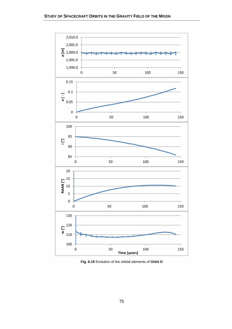
STUDY OF SPACECRAFT ORBITS IN THE GRAVITY FIELD OF THE MOON
75
Fig. 6.19 Evolution of the orbital elements of Orbit O
1,990.0
1,995.0
2,000.0
2,005.0
2,010.0
0 50 100 150
a[m
]
0
0.05
0.1
0.15
0 50 100 150
e [
-]
85
90
95
100
0 50 100 150
i [°
]
0
5
10
15
20
0 50 100 150
RA
AN
[°]
100
110
120
130
0 50 100 150
w [
°]
Time [years]
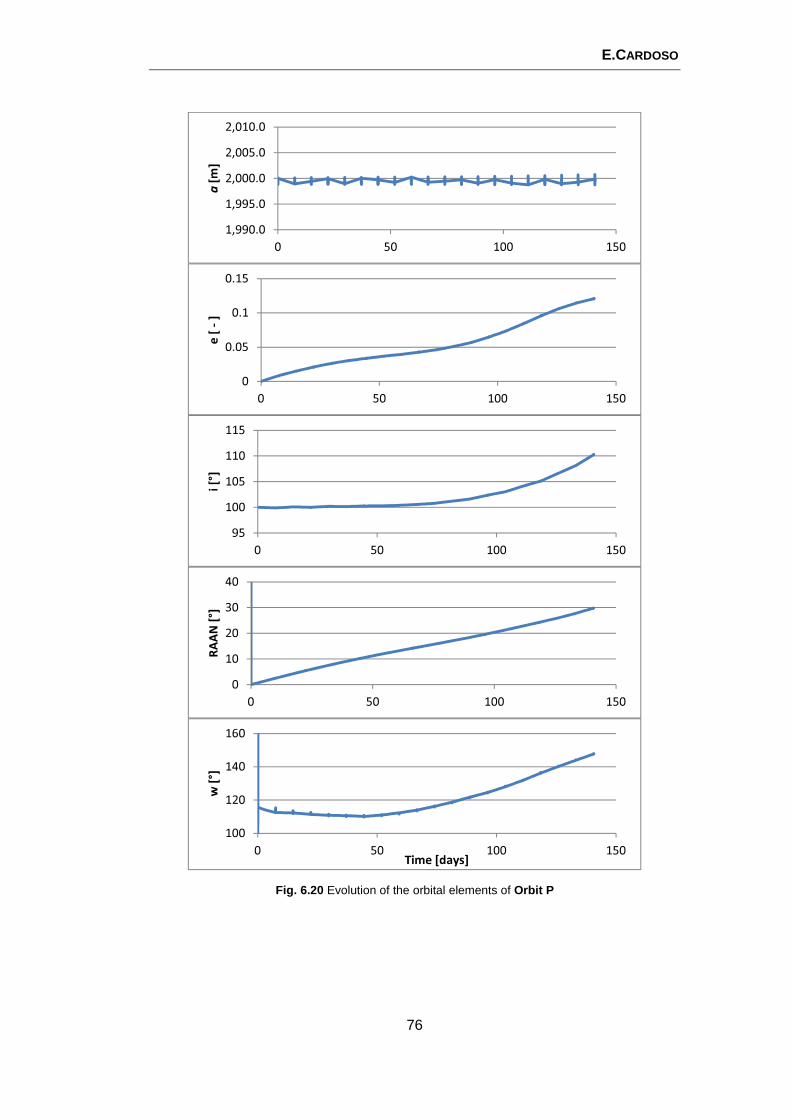
E.CARDOSO
76
Fig. 6.20 Evolution of the orbital elements of Orbit P
1,990.0
1,995.0
2,000.0
2,005.0
2,010.0
0 50 100 150
a[m
]
0
0.05
0.1
0.15
0 50 100 150
e [
-]
95
100
105
110
115
0 50 100 150
i [°
]
0
10
20
30
40
0 50 100 150
RA
AN
[°]
100
120
140
160
0 50 100 150
w [
°]
Time [days]
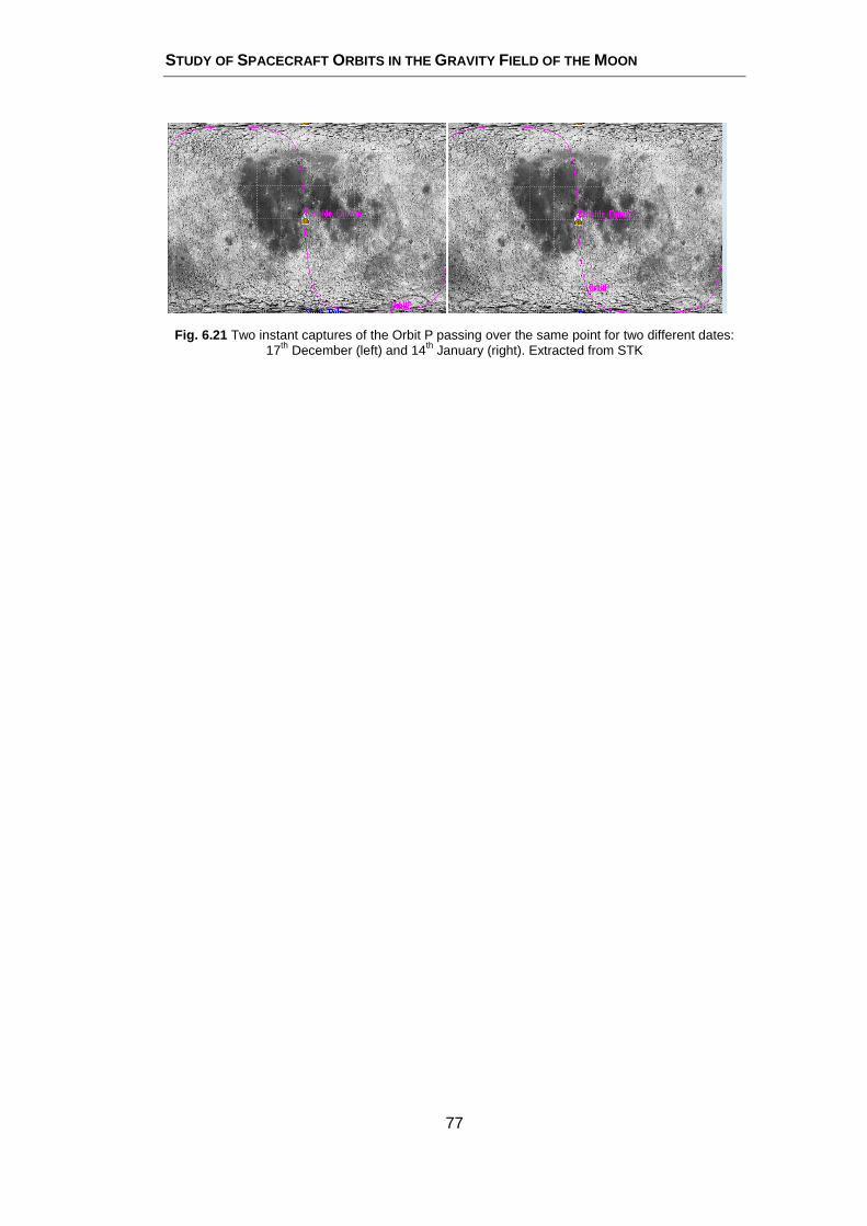
STUDY OF SPACECRAFT ORBITS IN THE GRAVITY FIELD OF THE MOON
77
Fig. 6.21 Two instant captures of the Orbit P passing over the same point for two different dates: 17th December (left) and 14th January (right). Extracted from STK

E.CARDOSO
78
CHAPTER SEVEN.
CONCLUSIONS AND FUTURE WORK
This study is the analysis of the evolution of low lunar orbits under the
gravitational potential of the Moon and additional perturbations of gravitational
(Earth and Sun gravity) and non-gravitational (radiation pressure) nature. Such
evolution can be used to estimate the amount of propellant required to maintain a
certain orbit during a given time or, alternatively as in the present case, to identify
orbits which may offer a wide surface coverage without orbit correction
maneuvers.
The analysis of the perturbations acting on a probe in low lunar orbit has
shown the relative importance of solar radiation pressure, albedo radiation
pressure, planetary infrared radiation pressure and third body (Earth and Sun)
gravitational effects with respect to the gravitational acceleration due to the lunar
mass distribution (see Fig. 4.5). The latter has been modeled in spherical
harmonics with the Stokes coefficients of the LP100K model.
The work is distributed over three areas:
• The extension of the basic code developed by [5] mainly to include
numerical integration capabilities, model the perturbations other than the
lunar gravity field and rearrange the computation of the lunar gravitational
acceleration with the lumped coefficients approach.
• The identification of initial conditions of lunar orbits of interest for specific
applications (in the field of reconnaissance, mapping, communications
and navigation) based on the study of the literature.
• Simulation and analysis of the evolution of a set of such orbits to estimate
surface coverage and lifetime.
The validation of the enhanced code has consisted in simulating a Keplerian
orbit, an orbit affected by the second zonal harmonic only, and specific orbits
found in the literature.
The application orbits have been divided into three categories: frozen orbits,
RGT orbits and polar orbits. Each type offers its own benefits and can be used in
specific types of missions. Among the frozen orbits, which are characterized by
high stability, Orbit J looks interesting because of its low altitude (semi-major
axis = 1861[V�]) and because it avoids impact for nearly two months without
maneuvering. This kind of orbits could be useful for scientific observation.
STUDY OF SPACECRAFT ORBITS IN THE GRAVITY FIELD OF THE MOON
79
RGT orbits provide even higher stability. In the context of lunar
communications and navigations, one such orbit could be shared by three
satellites, 120° apart in true anomaly. The inclination of Orbit B makes it
especially suitable for this purpose, with a very good coverage of the South Pole.
Finally, polar orbits are suitable for mapping, observation, and
reconnaissance. We find that orbits between 95° and 100° do not impact for long
times: an orbit with an inclination of 95°, such as Orbit O, stays close to the pole
without maneuvers for longer times.
Future work includes further enhancement and improvement of the code.
Some simplifying assumptions can be released in favor of more accurate
modeling: for example, the modeling of the orbits of the Moon, the Sun and the
Earth and the hypothesis concerning the initial alignment of the three bodies.
Improvements can be applied to the representation of the perturbations and the
inclusion of the third body effect of other bodies, such as Jupiter. At some point
the representation of the state vector of the planets should be given by the real
ephemerides. Concerning the simulations, an important future action is the
inclusion of orbital maneuvers and the development of an optimized strategy for
orbit maintenance. This action would make the tool complete and convert it into a
solid and fundamental instrument for mission design.
E.CARDOSO
80
APPENDIX A.
LUNAR DATA
This appendix contains information about the gravity model coefficients. We
start by giving an overview of the LP mission with details on the Doppler Gravity
Experiment (DGE) which was the responsible for the gravity field measurements
that took to the estimation of the Stokes coefficients.
A.1 LUNAR PROSPECTOR
Lunar Prospector was launched on January 6, 1998 and placed, after a series
of maneuvers, in a near circular lunar orbit on January 15 at an altitude of 100
km. LP remained in this polar orbit for about one year, i.e., for the duration of the
nominal mission. This ensured global coverage for the gravity experiment with a
periodicity of 14 days, except when the spacecraft disappeared behind the Moon.
On December 19 1988, the altitude of LP was reduced to an average of 40 km to
calibrate the gravity field in preparation for an even lower extended mission. LP
began its extended mission on January 29 1999, when the spacecraft was
lowered to an average altitude of 30 km to obtain higher resolution gravity,
spectrometric and magnetic data. At the end of the mission on July 31 1999, the
LP spacecraft impacted with the lunar surface in an unsuccessful attempt to
detect water vapor in the rising dust from impact.
Since there has been no direct observation of the lunar gravity of the far side
by any lunar mission, tracking data from all missions prior to LP have provided
important information concerning the lower degree harmonics and large-scale
features in that area. In fact, the far side gravity information comes from the
observed long-term effect on the spacecraft orbit. This far side hole in the gravity
data was by far the biggest challenge in processing all the lunar gravity data and
obtaining a reasonable gravity solution.
The DGE of LP helped improving the models of the Moon’s gravitational field.
As said in Chapter 1, the Moon has a much “bumpier” gravitational field than the
Earth, with small anomalies due to mascons on the surface and a large
asymmetry due to the fact that the crust is thicker on the far side of the Moon.
These bumps cause an orbiting spacecraft to speed up or slow down.
STUDY OF SPACECRAFT ORBITS IN THE GRAVITY FIELD OF THE MOON
81
The DGE drew a map of the bumps and, unlike the other experiments aboard
LP, required no extra instrumentation. All of the data was collected simply by
communicating with the spacecraft. As the spacecraft orbited the Moon in a polar
orbit, its speed could always be determined from the Earth by the Doppler effect.
By tracking the velocity of the spacecraft, mission scientists could infer the forces
acting upon it. For over 99 percent of the duration of the mission (except only
periods when the engines were being fired), the only force on LP was the gravity.
Passive 3-way Doppler measurements were collected by DLR’s 30 m antenna
whenever LP was visible from Weilheim, and uplinks were provided by NASA’s
Deep Space Network (DSN). The measurement principle, a 3-way Doppler
tracking, differs from the common 2-way measurements by using separate uplink
and downlink stations.
Thus, by simply circling the Moon and sending signals back to Earth, LP
mapped the Moon’s gravitational field. LP completed its gravitational map in two
months. However, the results of the DGE were greatly improved with the
extended mission beyond the first year.
Historical tracking data from the LO and Apollo missions in the mid-1960s to
early 1970s, as well as more recent data from the 1994 Clementine mission,
yielded a generally low-resolution representation of lunar gravity fields. DGE
provided the first polar low altitude measurement of the lunar gravity field. This
provided the spacecraft with the first truly operational gravity map of the Moon
and immediately improved orbit and fuel efficiency. Improved gravity information
has not only helped scientists build better models of the role of impact processes
on the history and evolution of the Moon, but has also helped in estimating the
lunar core size and metallic iron content. A more practical benefit of the lunar
gravity data provided by the DGE experiment was that a more precise gravity
map of the Moon could aid future mission planners in computing fuel-efficient
journeys to the Moon, and may even help identify potential resources.
LP’s high quality gravity data, improved by roughly a factor five over previous
estimates, indicated the existence of a lunar core, probably of iron, with a radius
of more than 300 km. Such improvements to the lunar gravity field also offered
the practical benefits of modeling long-term spacecraft orbits about the Moon,
which allowed more accurate planning of future mission fuel needs, and enabled
the development of fuel efficient orbital maintenance strategies.
For further information about LP spacecraft and mission, the reader is
referred to [2].
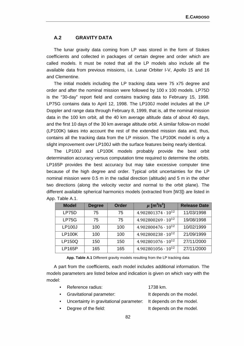
E.CARDOSO
82
A.2 GRAVITY DATA
The lunar gravity data coming from LP was stored in the form of Stokes
coefficients and collected in packages of certain degree and order which are
called models. It must be noted that all the LP models also include all the
available data from previous missions, i.e. Lunar Orbiter I-V, Apollo 15 and 16
and Clementine.
The initial models including the LP tracking data were 75 x75 degree and
order and after the nominal mission were followed by 100 x 100 models. LP75D
is the “30-day” report field and contains tracking data to February 15, 1998.
LP75G contains data to April 12, 1998. The LP100J model includes all the LP
Doppler and range data through February 8, 1999, that is, all the nominal mission
data in the 100 km orbit, all the 40 km average altitude data of about 40 days,
and the first 10 days of the 30 km average altitude orbit. A similar follow-on model
(LP100K) takes into account the rest of the extended mission data and, thus,
contains all the tracking data from the LP mission. The LP100K model is only a
slight improvement over LP100J with the surface features being nearly identical.
The LP100J and LP100K models probably provide the best orbit
determination accuracy versus computation time required to determine the orbits.
LP165P provides the best accuracy but may take excessive computer time
because of the high degree and order. Typical orbit uncertainties for the LP
nominal mission were 0.5 m in the radial direction (altitude) and 5 m in the other
two directions (along the velocity vector and normal to the orbit plane). The
different available spherical harmonics models (extracted from [W3]) are listed in
App. Table A.1.
Model Degree Order o [m 3/s2] Release Date
LP75D 75 75 4.902801374 · 10� 11/03/1998
LP75G 75 75 4.902800269 · 10� 19/08/1998
LP100J 100 100 4.902800476 · 10� 10/02/1999
LP100K 100 100 4.902800238 · 10� 21/09/1999
LP150Q 150 150 4.902801076 · 10� 27/11/2000
LP165P 165 165 4.902801056 · 10� 27/11/2000
App. Table A.1 Different gravity models resulting from the LP tracking data
A part from the coefficients, each model includes additional information. The
models parameters are listed below and indication is given on which vary with the
model:
• Reference radius: 1738 km.
• Gravitational parameter: It depends on the model.
• Uncertainty in gravitational parameter: It depends on the model.
• Degree of the field: It depends on the model.
STUDY OF SPACECRAFT ORBITS IN THE GRAVITY FIELD OF THE MOON
83
• Order of the field: It depends on the model.
• Normalization state: 1.
• Reference longitude: 0.0.
• Reference latitude: 0.0.
It must be noted that all the parameters that vary are listed in App. Table A.1
except the uncertainty in the gravitational parameter. Nevertheless, the largest is
seven orders of magnitude below the gravitational parameter, so it has been
neglected when using the constant for the computations. As an additional point,
the normalization state can get three different values, 0, 1 or 2 which means
respectively that the coefficients are unnormalized, fully normalized or other. In
the model each row in the table contains the degree index �, the order index �,
the coefficients ��� and +��, and the uncertainties in ���and +��. The delimited
data require 107 ASCII characters; these are followed by a pad of 13 unspecified
ASCII characters, an ASCII carriage-return, and an ASCII line-feed. All this
information about has been extracted from [18].
To sum up, the model selected for the present study in order to met a
compromise between time computations and precision has been LP100K. Note
that this same model is available when simulating by means of STK.
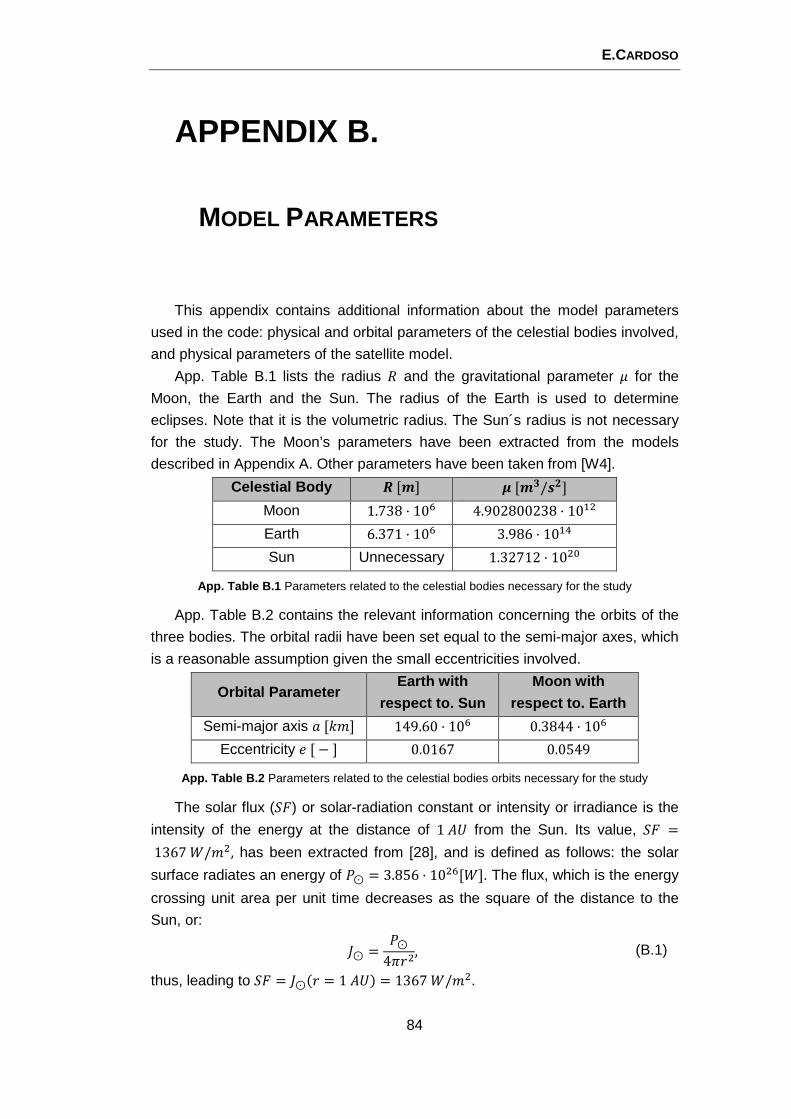
E.CARDOSO
84
APPENDIX B.
MODEL PARAMETERS
This appendix contains additional information about the model parameters
used in the code: physical and orbital parameters of the celestial bodies involved,
and physical parameters of the satellite model.
App. Table B.1 lists the radius I and the gravitational parameter � for the
Moon, the Earth and the Sun. The radius of the Earth is used to determine
eclipses. Note that it is the volumetric radius. The Sun´s radius is not necessary
for the study. The Moon’s parameters have been extracted from the models
described in Appendix A. Other parameters have been taken from [W4].
Celestial Body p[\] o[\6/i7] Moon 1.738 · 10! 4.902800238 · 10�
Earth 6.371 · 10! 3.986 · 10�/
Sun Unnecessary 1.32712 · 10�
App. Table B.1 Parameters related to the celestial bodies necessary for the study
App. Table B.2 contains the relevant information concerning the orbits of the
three bodies. The orbital radii have been set equal to the semi-major axes, which
is a reasonable assumption given the small eccentricities involved.
Orbital Parameter Earth with
respect to. Sun
Moon with
respect to. Earth
Semi-major axis �[V�] 149.60 · 10! 0.3844 · 10!
Eccentricity �[−] 0.0167 0.0549
App. Table B.2 Parameters related to the celestial bodies orbits necessary for the study
The solar flux (+L) or solar-radiation constant or intensity or irradiance is the
intensity of the energy at the distance of 1�� from the Sun. Its value, +L =1367M/�, has been extracted from [28], and is defined as follows: the solar
surface radiates an energy of �⊙ = 3.856 · 10![M]. The flux, which is the energy
crossing unit area per unit time decreases as the square of the distance to the
Sun, or:
�⊙ =�⊙4>$, (B.1)
thus, leading to +L = �⊙�$ = 1��� = 1367M/�.
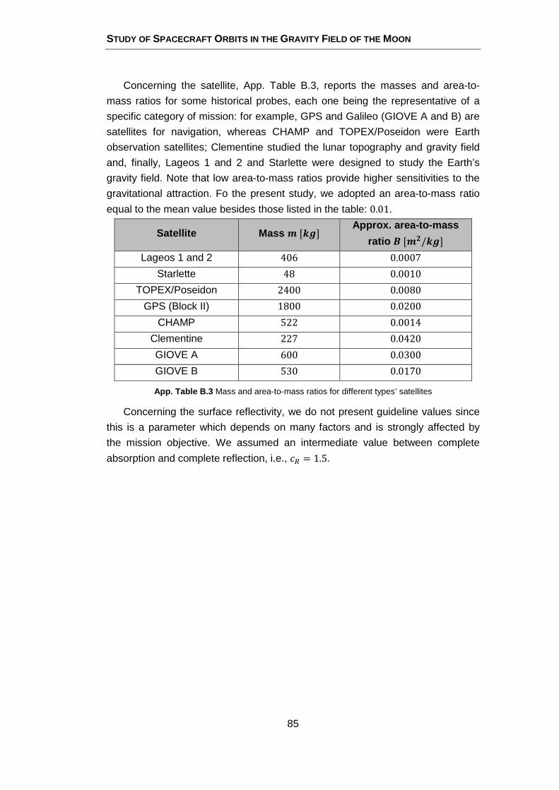
STUDY OF SPACECRAFT ORBITS IN THE GRAVITY FIELD OF THE MOON
85
Concerning the satellite, App. Table B.3, reports the masses and area-to-
mass ratios for some historical probes, each one being the representative of a
specific category of mission: for example, GPS and Galileo (GIOVE A and B) are
satellites for navigation, whereas CHAMP and TOPEX/Poseidon were Earth
observation satellites; Clementine studied the lunar topography and gravity field
and, finally, Lageos 1 and 2 and Starlette were designed to study the Earth’s
gravity field. Note that low area-to-mass ratios provide higher sensitivities to the
gravitational attraction. Fo the present study, we adopted an area-to-mass ratio
equal to the mean value besides those listed in the table: 0.01.
Satellite Mass \[[q] Approx . area-to-mass
ratio r[\7/[q] Lageos 1 and 2 406 0.0007
Starlette 48 0.0010
TOPEX/Poseidon 2400 0.0080
GPS (Block II) 1800 0.0200
CHAMP 522 0.0014
Clementine 227 0.0420
GIOVE A 600 0.0300
GIOVE B 530 0.0170
App. Table B.3 Mass and area-to-mass ratios for different types’ satellites
Concerning the surface reflectivity, we do not present guideline values since
this is a parameter which depends on many factors and is strongly affected by
the mission objective. We assumed an intermediate value between complete
absorption and complete reflection, i.e., �� = 1.5.
E.CARDOSO
86
APPENDIX C.
NUMERICAL SOLVER
C.1 INTRODUCTION TO NUMERICAL ODE METHODS
Amongst the many methods for numerically integrating ordinary differential
equations (ODE), there are the Euler’s method, the Heun’s method and the
classic 2nd to 4th Runge-Kutta methods [31]. The step size ℎ in the first two is
constant, which may lead to excessive error when dealing with either high-speed
trajectories or astrophysical equations. Furthermore, the method’s order N means
that the local truncation error is s�ℎ8���. A good ODE integrator should be capable of exerting some adaptive control
over the whole integration process, making frequent changes in the step size and
in order to meet a pre-established accuracy in the solution with as little
computational effort as possible. The most straightforward and used solver which
meets this definition is the Runge-Kutta of 4th order. Its popularity lies in the fact
that the higher the order is, the larger the number of evaluations requires, but
never more than N + 2 evaluations. Some rough strategies have been used to
increase one order higher than four by advancing from � to � + 2ℎ, which gives
estimates of 5th order accuracy. Nevertheless, there was no way to monitor the
truncation error [25], which means that a higher order does not necessarily mean
a higher accuracy.
Taking that into account, an alternative variable step size algorithm to the
conventional Runge-Kutta’s one was necessary to be found whenever a higher
order was required. That algorithm was indeed found by Fehlberg, who initially
discovered a 5th order method with 6 function evaluations, say V� where � =1,2,… ,6, as well as a combination of the six functions that gives a 4th order
method (this one is called the embedded 4th order formula, in this particular
case). The difference between the two estimates of the function evaluated at � + ℎ can be used as an estimate of the truncation error in the adjustment of the
step size.
This efficient method, which improves the 4th Runge-Kutta method providing
an estimate of the truncation error for higher orders, has been further increased
to higher orders. Below we illustrate the Runge-Kutta-Fehlberg 7(8), adopted in
STUDY OF SPACECRAFT ORBITS IN THE GRAVITY FIELD OF THE MOON
87
this study to determine the evolution of the position of a low-altitude orbiting
satellite around the Moon.
C.2 RUNGE-KUTTA-FEHLBERG METHOD
Let consider a general initial value problem (IVP) ����� = W��,��, ����� = ��. (C.1)
Now consider the following equations
W� = W���,���, (C.2)
W9 = W t�� + u9 ,�� + ℎ?Q9 W 9��
��
v, (C.3)
where w = 1,2,… ,I and = 1,2,… ,I − 1. Then, the ���� + ℎ� must satisfy
���� + ℎ� = �� + ℎ?�9W9�
9��
+ s�ℎ8���, (C.4)
where �9 and I are chosen so as to meet the order of the method N. The
constants Q9 and W are to be found as well; they are, nevertheless, already
tabulated depending upon the desired order of the method. If s�ℎ8��� is not
considered Eq. (C.4) would show ��. This is valid for any Runge-Kutta method
regardless its order.
Let us now include the embedded equation that Fehlberg proposed to have
control of the estimate of the truncation error:
�x��� + ℎ� = �� + ℎ?�̂9W9�:
9��
+ sJℎ8;��K, (C.5)
where the W9 are the same as before, but �̂9 are new coefficients (already known).
This equation must have a truncation error whose order is higher than the order
of Eq. (C.4), N̂ > N; thus, the local error of truncation, namely �z, that will let the
solver to adapt the size step at new numerical integration step is
�z = ���� + ℎ�− �x��� + ℎ�. (C.6)
C.3 RUNGE-KUTTA-FEHLBERG METHOD OF ORDER 7(8)
The adopted Runge-Kutta-Fehlberg method has an order of 7(8): a variable
step size method of order 7th with an 8th order error estimate, used to change the
step size during the integration. The formulae are as follows
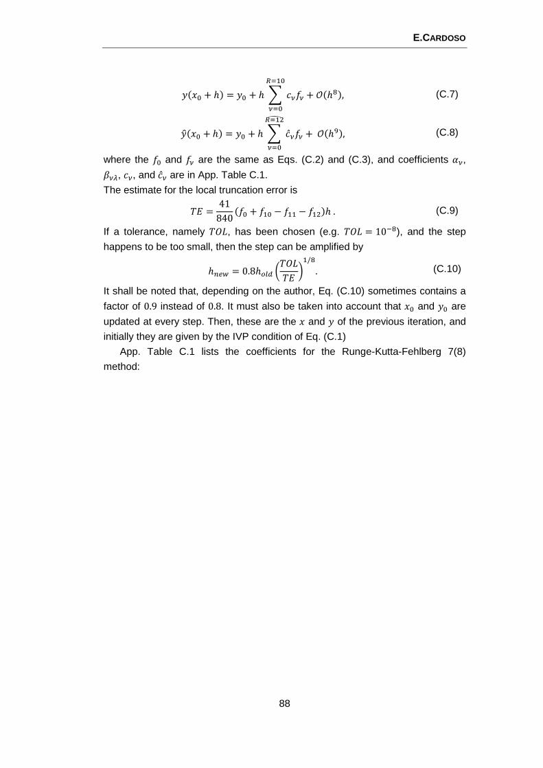
E.CARDOSO
88
���� + ℎ� = �� + ℎ ? �9W9 + s�ℎ �����
9��
, (C.7)
�x��� + ℎ� = �� + ℎ ? �̂9W9���<
9��
+ s�ℎ=�, (C.8)
where the W� and W9 are the same as Eqs. (C.2) and (C.3), and coefficients u9, Q9 , �9, and �̂9 are in App. Table C.1.
The estimate for the local truncation error is
�z =41
840�W� + W�� − W�� − W��ℎ. (C.9)
If a tolerance, namely �1Y, has been chosen (e.g. �1Y = 10� ), and the step
happens to be too small, then the step can be amplified by
ℎ��> = 0.8ℎ?@A 4�1Y�z 5�/ . (C.10)
It shall be noted that, depending on the author, Eq. (C.10) sometimes contains a
factor of 0.9 instead of 0.8. It must also be taken into account that �� and �� are
updated at every step. Then, these are the � and � of the previous iteration, and
initially they are given by the IVP condition of Eq. (C.1)
App. Table C.1 lists the coefficients for the Runge-Kutta-Fehlberg 7(8)
method:
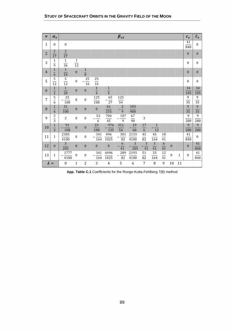
STUDY OF SPACECRAFT ORBITS IN THE GRAVITY FIELD OF THE MOON
89
{ |B }BC ~B ~xB 1 0 0
41
840 0
2 2
27
2
27 0 0
3 1
9
1
36
1
12 0 0
4 1
6
1
24 0
1
8 0 0
5 5
12
5
12 0 −
25
16
25
16 0 0
6 1
2
1
20 0 0
1
4
1
5
34
105
34
105
7 5
6 −
25
108 0 0
125
108 −
65
27
125
54
9
35
9
35
8 1
6
31
100 0 0 0
61
255 −
2
9
103
900
9
35
9
35
9 2
3 2 0 0 −
53
6
704
45 −
107
9
67
90 3
9
280
9
280
10 1
3 −
91
108 0 0
23
108 −
976
135
311
54 −
19
60
17
6 −
1
12
9
280
9
280
11 1 2383
4100 0 0 −
341
164
496
1025 −
301
82 2133
4100
45
82
45
164
18
41
41
840 0
12 0 3
205 0 0 0 0 −
6
41 −
3
205 −
3
41
3
41
6
41 0 0
41
840
13 1 −1777
4100 0 0 −
341
164 4496
1025 −
289
82 2193
4100
51
82
33
164
12
41 0 1 0
41
840
� = 0 1 2 3 4 5 6 7 8 9 10 11
App. Table C.1 Coefficients for the Runge-Kutta-Fehlberg 7(8) method
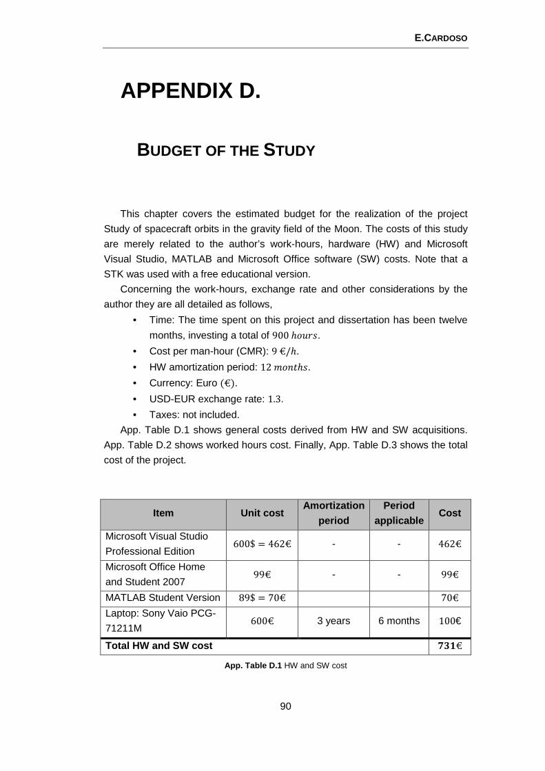
E.CARDOSO
90
APPENDIX D.
BUDGET OF THE STUDY
This chapter covers the estimated budget for the realization of the project
Study of spacecraft orbits in the gravity field of the Moon. The costs of this study
are merely related to the author’s work-hours, hardware (HW) and Microsoft
Visual Studio, MATLAB and Microsoft Office software (SW) costs. Note that a
STK was used with a free educational version.
Concerning the work-hours, exchange rate and other considerations by the
author they are all detailed as follows,
• Time: The time spent on this project and dissertation has been twelve
months, investing a total of 900ℎS $F. • Cost per man-hour (CMR): 9€/ℎ.
• HW amortization period: 12�S��ℎF. • Currency: Euro (€).
• USD-EUR exchange rate: 1.3.
• Taxes: not included.
App. Table D.1 shows general costs derived from HW and SW acquisitions.
App. Table D.2 shows worked hours cost. Finally, App. Table D.3 shows the total
cost of the project.
Item Unit cost Amortization
period
Period
applicable Cost
Microsoft Visual Studio
Professional Edition 600$ = 462€ - - 462€
Microsoft Office Home
and Student 2007 99€ - - 99€
MATLAB Student Version 89$ = 70€ 70€
Laptop: Sony Vaio PCG-
71211M 600€ 3 years 6 months 100€
Total HW and SW cost ��b€
App. Table D.1 HW and SW cost
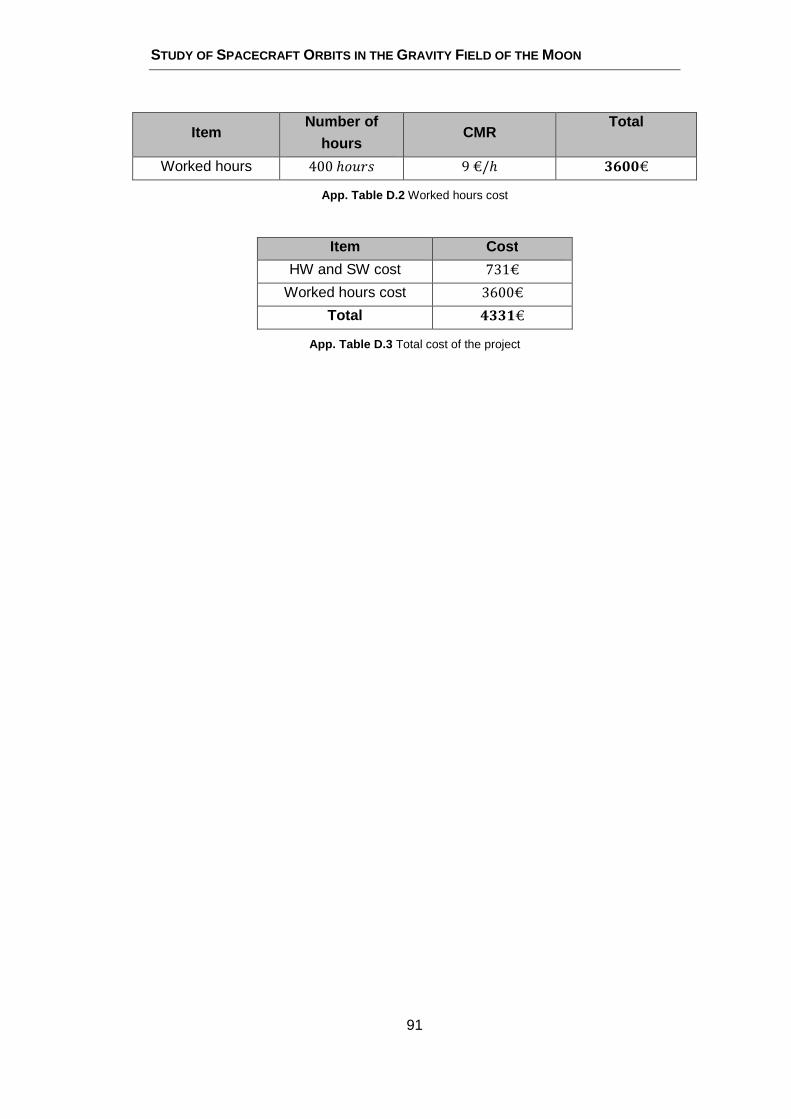
STUDY OF SPACECRAFT ORBITS IN THE GRAVITY FIELD OF THE MOON
91
Item Number of
hours CMR
Total
Worked hours 400ℎS $F 9€/ℎ ��gg€
App. Table D.2 Worked hours cost
Item Cost
HW and SW cost 731€
Worked hours cost 3600€
Total ���b€
App. Table D.3 Total cost of the project
E.CARDOSO
92
REFERENCES
The references below are shown in alphabetical order and divided into two sections, one concerning books, lecture and articles, and another one for websites.
BOOKS, LECTURES AND ARTICLES
[1] Akim, E., “Determination of the Gravity Field of the Moon by the Motion of
Luna-10”; Dokl. Akad. Nauk SSSR, 160, 799-802 (1996).
[2] Andolz, F.J., “Lunar Prospector Mission Handbook” (1998).
[3] Bate, R.R., Mueller, D.D., White, J.E., “Fundamentals of Astrodynamics”;
Dover Publications, New York (1971).
[4] Casotto, S., Fantino, E., “Gravitational gradients by tensor analysis with
application to spherical coordinates”; Journal of Geodesy, 83(7), 621-634
(2008).
[5] Casotto, S., Fantino, E., “Methods of harmonic synthesis for global
geopotentinal models and their first-, second- and third-order gradients”
(2008).
[6] Chobotov, V.A., “Orbital Mechanics”; 3rd Edition, AIAA, Reston, Virginia
(2002)
[7] Cunningham, L.E., “On the computation of the spherical harmonic terms
needed during the numerical integration of the orbital motion of an artificial
satellite”; Celestial Mech, 2, 207-216 (1970).
[8] Danby, J.M.A., “Fundamentals of Celestial Mechanics”; Willmann-Bell,
Richmond, Virgina (1992).
STUDY OF SPACECRAFT ORBITS IN THE GRAVITY FIELD OF THE MOON
93
[9] Davis, J., “Lunar Gravitational Field Estimation and the Effects of
Mismodeling upon Lunar Satellite Orbit Prediction”; Cambridge, MIT (1993).
[10] Ely, T.A., Lieb, E., “Constellations of Elliptical Inclined Lunar Orbits Providing
Polar and Global Coverage”; AAS, 05-343 (2005).
[11] Ely, T.A., “Stable Constellations of Frozen Elliptical Inclined Lunar Orbits”;
Journal of the Astronautical Sciences, Vol. 53, No. 3, 301-316 (2005).
[12] Garrick-Bethell, I., et al., “Early Lunar Magnetism”; Science 323 (5912), 356-
359 (2009).
[13] Holmes, S.A., Featherstone, W.E., “A unified approach to the Clenshaw
summation and the recursive computation of very high degree and order
normalized associated Legendre functions”; J Geod, 76, 279-299 (2002).
[14] Holmes, S.A., Featherstone, W.E., “Short Note: extending simplified high-
degree synthesis methods to second latitudinal derivatives of geopotential”; J
Geod, 76, 279-299 (2002).
[15] Kaplan, M.H., “Modern Spaceraft Dynamics and Control”. Wiley (1976).
[16] Kaula, W.M., “Theory of Satellite Geodesy”; Dover (2000).
[17] Konopliv, A.S., et al., “Improved Gravity Field of the Moon from Lunar
Prospector”; Science, 281, 1476-1480 (1998).
[18] Konopliv, A.S., et al., “Recent Gravity Models as a Result of the Lunar
Prospector Mission”; Icarus, 150, 1-18 (2001).
[19] Lara. M, Elipe, A., “Frozen Orbits in the Tesseral Artificial Satellite Theory”;
Space Flight Dynamics, Proceedings of the 12th International Symposium,
397 (1997).
[20] Lara. M, et al., “Preliminary Design of Low Lunar Orbits”:
http://desaedeleer.org/ber-008.pdf. Last visited on December 2011.
E.CARDOSO
94
[21] Larson, W.J., Wertz, J.R., “Space Mission Analysis and Design”; Space
Technology Library, Microcosm Press (1992).
[22] Matthews, G., “Celestial body irradiance determination from an underfilled
satellite radiometer: application to albedo and thermal emission
measurements of the Moon using CERES”; Appl. Opt. 47, 4981-4993 (2008).
[23] Metris, G., Xu, J., Wytrzyszczak, I., “Derivatives of the gravity potential with
respect to rectangular coordinates”; Celestial Mech Dyn Astron, 71, 137-151
(1999).
[24] Pines, S., “Uniform representation of the gravitational potential and its
derivatives”; AIAA J 11, 1508-1511 (1973).
[25] Press, W.H., Teukolsky, S.A., Vetterlin, W.T., “Numerical recipes in C: The art
of scientific computing”; Cambridge University Prees, Cambridge (1992).
[26] Russell, R.P., Lara, M., “Repeat Ground Track Lunar Orbits in the Full-
Potential Plus Third-Body Problem”; AIAA (2006).
[27] Torge, W., “Geodesy”; Walter de Gruyter, Berlin (2001).
[28] Vallado, D.A., “Fundamentals of Astrodynamics and Applications”; Space
Technology Library, Microcosm Press (2007).
[29] Wertz, R.J., “Spacecraft Attitude Determination and Control”; London (1978).
[30] Wieczorek, M.A., Gravity and topography of the terrestrial planets, Treatise
on Geophysics, 10, 165-205, doi:10.1016/B978-044452748-6/00156-5
(2007).
[31] Zadunaisky, P.E., “Sistemas dinámicos, teorías y métodos numéricos
computacionales”; Dpt. Of Mathematics – Buenos Aires University, Buenos
Aires (2009).
STUDY OF SPACECRAFT ORBITS IN THE GRAVITY FIELD OF THE MOON
95
WEBSITES
[W1] A New Paradigm for Lunar Orbits. Last visited on January 2012
<http://science.nasa.gov/science-news/science-at-nasa/2006/30nov_highorbit/>
[W2] Bizarre Lunar Orbits. Last visited on December 2011
<http://science.nasa.gov/science-news/science-at-nasa/2006/06nov_loworbit/>
[W3] PDS Geosciences Node Data and Services; Lunar Prospector. Last visited on
December 2011 <http://pds-geosciences.wustl.edu/missions/lunarp/index.htm>
[W4] Planetary Fact Sheet – Metric. Last visited on December 2011
<http://nssdc.gsfc.nasa.gov/planetary/factsheet/>
[W5] Spudis Lunar Resources – SLR. Last visited on December 2011
<http://www.spudislunarresources.com/Images_Maps.htm>
The Register – Highest Point on the Moon. Last visited on January 2012
<http://www.theregister.co.uk/2010/10/29/highest_point_on_moon/>