EDGE-BASED PARTITION CODING FOR

FRACTAL IMAGE COMPRESSION

Tilo Ochotta and Dietmar Saupe

Department of Computer and Information Science

University of Konstanz, Germany

ABSTRACT

This paper presents an approach for fractal image compression that yields the best performance compared to

fractal methods that do not rely on hybrid transform coding. The achievement is obtained using the standard

algorithm in which the image is partitioned into non-overlapping range blocks which are approximated by corre-

sponding larger domain blocks with image intensities that are affinely similar to those of the range blocks. The

particular feature of our approach is the adaptive spatial partition, that proceeds in a split/merge fashion. In

previous split/merge partitions for fractal image coding the merging started from a uniform partition consisting

of square blocks of equal size. In this paper we base the block merging on an adaptive quadtree partitioning. An

efficient encoding method for the quadtree-based split/merge partitions is proposed which generalizes the coding

of region edge maps and which includes special context modeling. The encoding method may be used for other

applications that rely on image partitions.

Key words: Fractal Image Compression, Partition Coding, Region Edge Maps, Image Segmentation.

1

EDGE-BASED PARTITION CODING FORFRACTAL IMAGE COMPRESSION

1 INTRODUCTION

Fractal image compression was conceived by Barnsley and Sloan [1, 2], and the first fully automated fractal

image compression algorithm was published by Jacquin in 1989 [3, 4]. Given an image, the encoder finds a

contractive affine image transformation (fractal transform) T such that the fixed point of T is close to the given

image in a suitable metric. The decoding is by iteration of the fractal transform starting from an arbitrary image.

Due to the contraction mapping principle, the sequence of iterates converges to the fixed point of T . Jacquin’s

original scheme showed promising results. Since then, many researchers have improved the original algorithm

outperforming standard JPEG image compression. However, the rate-distortion performance of current state-

of-the-art codecs based on wavelet transform coding as, e.g., in JPEG2000 cannot yet be reached even by the

best fractal coders that work in the spatial domain. For surveys, detailed discussions, computer code, and

bibliography see [5, 6, 7].

The fractal transform in its common form has two essential components, namely first, an image partition and

second, for each block of the partition (called range block) an address for a similar image block, called domain,

and a small set of real quantized transform parameters. These parameters determine an affine mapping of the

intensity values of the domain block that is shaped like the range block. These mappings are chosen such that

the intensities in each range block are approximated by the transformed intensities of the corresponding domain

block. The fractal transform T operates on an arbitrary image by mapping domains to ranges as specified in the

fractal code. Contractivity of the transform may be provided by a simple condition on one of the parameters of

the affine mappings.

Uniform image partitions do not yield satisfying rate-distortion performance for fractal coding. Thus, already

the first papers on fractal compression suggested adaptive image partitions. Jacquin used image squares that

were subdivided into smaller regions consisting of one to three subsquares of half the size [4]. In [5] adaptive

quadtrees were used. These partitions are built with square blocks which are recursively subdivided into four

subblocks of equal size until some approximation quality is reached or the block size falls below a given threshold.

Other hierarchical image partitions can be based on rectangles [8, 9] and polygons [10]. Delaunay triangulations

have also been used [11, 12].

Highly adaptive partitions can be generated by a split/merge scheme [13] in two phases. First, the image is

partitioned into successively smaller blocks until a termination criterion is fulfilled. Then neighboring regions

may be merged again as long as some coherence criterion is satisfied. In the methods in [14, 15, 16] the splitting

is simple and results in uniform square blocks. These small squares are merged again to form irregularly shaped

range blocks that adapt well to the structure of the underlying image and provide some of the best fractal coders

[16]. Uniform and quadtree partitions are easy to encode comprising just a small fraction of the total rate in a

fractal image code. However, more adaptive partitions such as those based on a split/merge process are harder to

encode efficiently. There are two main approaches. One may either encode the boundaries of the image regions,

or one can encode connectivity of the basic blocks that make up the image regions. Chain coding [17] belongs

to the first category, while region edge maps [18] are an example for the second kind.

Our work extends and improves the methods in [16] in two ways.

1. In 1976 Horowitz and Pavlidis [19] suggested a split/merge scheme for efficient image representation in

which the splitting provided a quadtree partition whose blocks are then merged to form adaptive image

regions. Such image partitions can also be generated when splitting all the way down to equal sized

squares. However, due to the occurrence of larger coherent blocks in the underlying quadtree partition a

2

more efficient code of the partition may be expected without significantly reducing the adaptivity of the

final partition. Thus, we propose to use this approach in the context of fractal coding. We note that this

has already been tried in [20, 21].

2. Our main contribution is an efficient method to encode the corresponding split/merge partition, i.e., an

image partition in which each block is the union of some neighboring square blocks from a given quadtree

partition, which must also be encoded efficiently. For this purpose we generalize the region edge maps

proposed in [18] and provide comprehensive context modelling for efficient arithmetic encoding.

The rest of the paper is organized as follows. In section 2 we briefly review the basics about fractal image

coding and give a short survey of previous work in the field of lossless partition coding that is relevant with

respect to our approach. In particular, we revisit region edge maps which provide the basis of our new method

for quadtree-based region edge maps. In section 3 we define a compression scheme for quadtree codes and

introduce quadtree-based region edge maps and their efficient encoding with context modelling. In section 4

we apply the proposed scheme to region-based fractal image compression providing efficient partition coding.

Experimental results are presented in section 5.

2 TERMINOLOGY AND RELATED WORK

2.1 Fractal Image Compression

We consider an image F of size N × N as a function that maps a set of N2 pixel coordinates (x, y),

x, y = 0, . . . , N − 1, to the set of grey values v ∈ {0, . . . , 255}. The function F may be represented as a

corresponding set of 3-tuples (x, y, v). A base block b is an n × n subset of F , b = {(x, y, v) ∈ F | x =

xmin, . . . , xmax, y = ymin, . . . , ymax} where xmax − xmin = ymax − ymin = n− 1. The base block size n is a fixed

parameter of our method and may be chosen as small as n = 1 amounting to base blocks being single pixels. For

our image partition we need to consider groups of connected base blocks as range blocks for the fractal coder.

We call two base blocks b1, b2, b1 ∩ b2 = ∅ adjacent, if and only if there are two pixels p1 = (x1, y1, v1) ∈ b1,

p2 = (x2, y2, v2) ∈ b2 such that |x2 − x1|+ |y2 − y1| = 1. We define a region as a connected set of base blocks. A

set of regions P = {ri | i = 0, . . . , nR − 1} with ri 6= rj and ri ∩ rj = ∅ for i 6= j which covers the image F , i.e.,

∪r∈P r = F , is called a partition of F .

The image F in a range block is approximated by an intensity transformed copy of a larger block, called

domain block. Let us denote by DF the domain image of size N/2×N/2 obtained by downsampling the original

N × N image F . Usually, downsampling proceeds by averaging intensity values of pixels in 2 × 2 blocks. For a

given range block r parameters xd, yd ∈ {0, . . . , N/2 − 1} and sr, or ∈ R are sought such that

v ≈ v = sr · DF ((x + xd) mod N/2, (y + yd) mod N/2) + or, (x, y, v) ∈ r, (2.1)

The region that is addressed with (xd, yd) in the domain image D and the same shape as the range block is the

domain block for the range r. The parameters sr and or allow scaling and adjustment of brightness of the grey

values of the domain. Scaling factors are chosen with the constraint |sr| < 1. Moreover, scaling factors sr and

offsets or are quantized for the purpose of encoding.

We also consider an approximation error for mapping (2.1):

E(r) =∑

(x,y,v)∈r

(v − v)2. (2.2)

The approximation error E(r) should be as small as possible. Typically, least squares optimization is used

to determine the best scaling factor and offset for a given domain address (xd, yd), and a search through a

3

0

2 3

1 NW N NE

XW X

NW N NE

W

(a) (b) (c)

Figure 1: Region edge maps with context modeling: (a) a block is represented by a symbol from {0, 1, 2, 3} whichencodes the presence resp. absence of region edges at the Northern and Western boundary of the block; (b) thesymbols of four preceding blocks (West, North West, North, and North East) are used to define a context; (c)the symbol combination N = 1, W = 2, X = 2 cannot occur in a partition.

pool of domains determines the domain which yields the least approximation error. We also consider a global

approximation error for the image F which is called collage error:

E = E(F, P ) =∑

r∈P

E(r). (2.3)

The fractal code must uniquely describe the image partition and for each range block in the partition the

domain block used together with the scaling factor and the offset. This code essentially amounts to the definition

of an image operator T . Given an image Ik, the transformed image Ik+1 = T (Ik) is obtained by applying all

range block transformations in (2.1), where the domain blocks are taken from the image Ik in place of F . This

image operator T is a contraction and, hence, iterating T starting with an arbitrary initial image I0 converges

to a unique image I⋆, the fixed point of the fractal transform T . The fixed point I⋆ can be constructed by the

decoder and serves as the image reconstruction. The reconstruction quality depends on the collage error 2.3,

which is due to the so-called collage theorem. For further details, background material, and proofs we refer to

the large body of literature, see, e.g., [5, 22, 23].

2.2 Lossless Partition Coding

There are two classes for lossless partition coding. The first one is chain coding in which sequences of symbols

for directions represent region boundaries [17]. A naive chain coding for image partitions encodes the closed

boundary of each region as a starting position and a sequence of steps in the directions North, East, South, and

West. This approach is not satisfying. The reason is that boundary segments are encoded twice because an

edge is shared by two neighboring regions except at the image boundary. Furthermore, the encoding of the start

positions can become expensive in bits even when the absolute address for a region is encoded relative to another

one. Several optimizations have been introduced, e.g., in [24], where three symbols are used to represent a chain

(go straight, left, or right). In [25] the partition is not coded as a set of closed region boundaries but as set of line

sequences. Each sequence describes a number of connected lines for which a relative starting point, the length

of each line, and the relative directions of the line segments are encoded. Each region edge is visited only once

and long straight lines can be encoded by a small number of symbols. Other, more sophisticated, methods for

chain coding (in the context of fractal image coding) are in our previous paper [26].

The second class of methods to represent region shapes is related to encoding binary images. A fundamental

method for compressing black-and-white images has been proposed in [27]. The binary intensities are encoded

individually in line-by-line order using an arithmetic coder [28] with context modelling. In [18], this approach

was extended to encode grid-based partitions in which the connectivity of a base block is encoded with one out

of four symbols each. For a given base block it suffices to indicate whether its Northern and Western borders

are part of a region boundary, which requires two bits per base block (see figure 1a). The resulting 4-nary image

is called a region edge map.

In [18] the symbols of a region edge map are encoded line-by-line with an adaptive arithmetic coder and

4

W NE N NW X

0 * 0 * 1

0 * 0 * 2

0 * 1 * 1

0 * 1 * 2

0 * 2 * 0

0 * 3 * 0

1 * 0 * 0

1 * 1 * 0

W NE N NW X

2 * 0 * 1

2 * 0 * 2

2 * 1 * 1

2 * 1 * 2

2 * 2 * 0

2 * 3 * 0

3 * 0 * 0

3 * 1 * 0

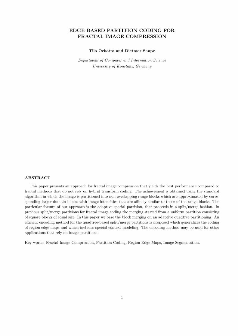
Table 1: Impossible symbol combinations. The asterisks correspond to any symbol {0, . . . , 3}. All in all 768 outof 45 = 1024 combinations may occur.

context modelling similar to [27]. The context modelling (figure 1b) uses four previously encoded/decoded

symbols (symbols for blocks in West, North West, North and North East direction). Due to elementary geometric

facts some symbol combinations cannot occur (figure 1c, table 1). Taking this into account the following formula

is proposed to update the probability p for a symbol z, that may appear in context c:

p(z|c) =λ · count(z|c) + 1

λ · count(c) + |Ac|, (2.4)

where count(z|c) is the number of symbols z encoded in context c, count(c) is the total number of occurrences of

context c, and |Ac| ≤ 4 is the number of symbols that are possible in context c. Probabilities p(z|c) for symbols

z that are not possible in context c as indicated in table 1 are set to zero. Following experimental results in

[18], the weight factor λ should be set to of 4 or 5 for best compression results. In our empirical studies we used

λ = 4.

3 PARTITION CODING METHOD

3.1 Quadtree Decomposition

Our partition method is based on a split/merge approach as introduced by Horowitz and Pavlidis in [19].

In our case, the splitting phase consists of a quadtree segmentation. Tate’s edge-based coding scheme [18] uses

a uniform grid of equally sized square base blocks. In this section we extend the coding to partitions in which

regions are unions of square base blocks from a quadtree segmentation.

A quadtree is a hierarchical data structure [29] amounting to an ordered tree with inner nodes of degree four.

In image processing applications a node corresponds to a rectangular (or square) image area, which is recursively

split into four equal size subrectangles (or subsquares) corresponding to the four children of the node. A split

rule evaluated for a given node, respectively the corresponding rectangle (square), determines termination of

the recursion in which case the node ends up as a leaf node of the quadtree. The blocks belonging to the leaf

nodes of the tree comprise the quadtree partition. By means of the split criterion the quadtree may adapt to

image content. For example, large blocks in low frequency areas and small blocks in high frequency areas can be

generated, respectively. Pseudo code for the procedure is given in algorithm 1.

After quadtree segmentation, an iterative merging phase follows where in each iteration two adjacent blocks

are merged, which may be further merged with other blocks in a succeeding iteration. An application specific

merge criterion, evaluated for each pair of adjacent blocks to be merged, determines two blocks that are merged

in an iteration step. Pseudo code for the procedure is given in algorithm 2.

5

During the merging process it is possible that a group of four blocks belonging to four child nodes of the same

parent node in the quadtree are merged into one region. In such a case it is possible to simplify the quadtree by

pruning it at the parent node. We call the resulting quadtree a fitted quadtree and expect to be able to encode

the fitted quadtree as well as the quadtree-based regions of the final image partition with a smaller rate.

Algorithm 1 split(n)

Input: quadtree leaf node n with corresponding image block r(n).Output: quadtree root node n with corresponding quadtree partition of r(n).• split criterion is given by boolean function SC(·).if SC(r(n)) then• expand the node n using four child nodes ni, i = 0, ..., 3for i=0,. . . ,3 do• ni = split(ni)

end forend ifreturn node n.

Algorithm 2 merge(P ,nR)

Input: quadtree partition P , target region number nR < |P |.Output: partition P ′ with |P ′| = nR regions.• Set P ′ = ∅.for all q ∈ P do• initialize q as region r• insert r into P ′

end forwhile |P ′| > nR do• find the region pair (ri, rj), ri, rj neighbors in P ′ minimizing an error criterion• insert ri ∪ rj into P ′

• remove ri and rj from P ′

end whilereturn P ′.

3.2 Quadtree Coding

In this subsection we describe the encoding of the quadtree partition. The following subsection covers the

encoding of the image partition derived from merging quadtree blocks. The (ordered) quadtree (figure 2a,b) is

traversed in depth-first order processing each node by outputting a binary symbol 1 for an inner node and 0 for a

leaf node. Since we also encode the smallest and largest depth of a leaf node as side information, we may delete

the symbols 1 for inner nodes above the minimal leaf depth and the symbols 0 for leaf nodes at the maximal

depth.

Context-based arithmetic coding is crucial for obtaining compact codes for quadtrees. For example, context

modelling can exploit the fact that situations given by one large quadtree block adjacent to many small quadtree

blocks (figure 2c) seldomly occur. For a given block q we consider the number of neighboring leaves in North

and West (zN and zW respectively). These numbers are known also at the decoder due to the depth-first

traversal of the quadtree. These counts are bounded, 0 ≤ zN , zW ≤ zmax, where zmax is determined by the

side information (minimal and maximal depth of leaf nodes). For example, zmax = 8 for a 4-32-quadtree, i.e., a

quadtree segmentation in which the minimal and maximal block sizes are 4 × 4 and 32 × 32, respectively.

We propose the following three heuristic schemes to build up a context for the given block q. In the last

subsection we empirically compare the performance of these three context models for quadtree partitions of

6

(a)

3 4

21q

(b) (c)

Figure 2: Quadtree decomposition after the top down scheme: (a) stepwise split up of the blocks; (b) encodingorder; (c) situation with low probability of occurrence: one block q has many neighbor blocks.

varying complexity for test images.

Full Context Two symbols are defined to be in the same context class if and only if the corresponding tuples

(zN , zW ) of neighbor leaf numbers are equal. If we number the context classes by c = 0, ..., cmax − 1, we

may write c = (zmax + 1)zN + zW and cmax = (zmax + 1)2.

Sum Context Two symbols are in the same context class if and only if the corresponding combined neighbor

leaf numbers, i.e., zN + zW , are equal. Thus, c = zN + zW and cmax = 2 · (zmax + 1).

Reduced Context Four context classes are defined by checking whether there are several neighboring leaf

nodes in the North and in the West. More precisely,

c =

0 for zN ≤ 1 and zW ≤ 1

1 for zN ≤ 1 and zW ≥ 2

2 for zN ≥ 2 and zW ≤ 1

3 for zN ≥ 2 and zW ≥ 2

and cmax = 4.

3.3 Quadtree-based Region Edge Maps

In this subsection we generalize the region edge map (REM) encoding scheme described in subsection 2.2 to

the case where the blocks used in the merging phase are from a quadtree image partition.

We assume that the encoding of the split/merge partition occurs after encoding the quadtree partition as

given in the last subsection 3.2. Thus, we may use the quadtree partition in the context modelling. We first note

that the split/merge partition based on merging blocks of the quadtree partition can easily be encoded using the

previous method for REM encoding when we define the region edge map in terms of a uniform image partition

consisting of atomic blocks of the size that is given by the smallest blocks that occur in the quadtree partition.

In other words, we imagine expanding the quadtree so that it becomes a full quadtree (all leaves have the same

depth) and define a symbol z ∈ {0, 1, 2, 3} for each leaf block depending on the presence of a region boundary

along its Western and Northern edges as before (figure 1a). We again encode the resulting symbol sequence

line by line from top to bottom and from left to right. Let us call this symbol sequence the quadtree-based

region edge map (QBREM). This sequence typically has many more symbols than there are blocks in the initial

quadtree partition. However, since the quadtree is available at the coder and the decoder we may use it in order

to design the context modelling to take advantage of this knowledge. For example, in this way the decoder is

able to completely determine many symbols from their context alone without any additional information.

7

hn ht

vt

vn

vt

hn

vn

hn

vn

vn

hnhn c

c

c

c c

c

i

iii

i ii

c

cc

c

c

c

i i i

ii

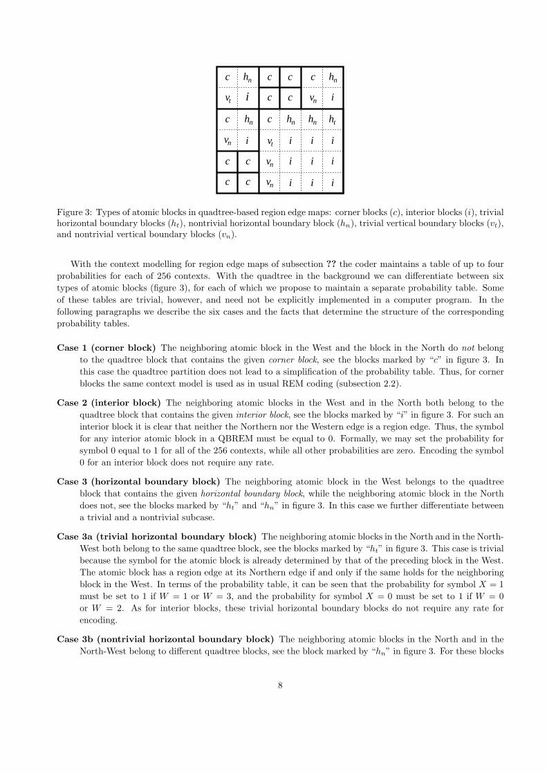
Figure 3: Types of atomic blocks in quadtree-based region edge maps: corner blocks (c), interior blocks (i), trivialhorizontal boundary blocks (ht), nontrivial horizontal boundary block (hn), trivial vertical boundary blocks (vt),and nontrivial vertical boundary blocks (vn).

With the context modelling for region edge maps of subsection ?? the coder maintains a table of up to four

probabilities for each of 256 contexts. With the quadtree in the background we can differentiate between six

types of atomic blocks (figure 3), for each of which we propose to maintain a separate probability table. Some

of these tables are trivial, however, and need not be explicitly implemented in a computer program. In the

following paragraphs we describe the six cases and the facts that determine the structure of the corresponding

probability tables.

Case 1 (corner block) The neighboring atomic block in the West and the block in the North do not belong

to the quadtree block that contains the given corner block, see the blocks marked by “c” in figure 3. In

this case the quadtree partition does not lead to a simplification of the probability table. Thus, for corner

blocks the same context model is used as in usual REM coding (subsection 2.2).

Case 2 (interior block) The neighboring atomic blocks in the West and in the North both belong to the

quadtree block that contains the given interior block, see the blocks marked by “i” in figure 3. For such an

interior block it is clear that neither the Northern nor the Western edge is a region edge. Thus, the symbol

for any interior atomic block in a QBREM must be equal to 0. Formally, we may set the probability for

symbol 0 equal to 1 for all of the 256 contexts, while all other probabilities are zero. Encoding the symbol

0 for an interior block does not require any rate.

Case 3 (horizontal boundary block) The neighboring atomic block in the West belongs to the quadtree

block that contains the given horizontal boundary block, while the neighboring atomic block in the North

does not, see the blocks marked by “ht” and “hn” in figure 3. In this case we further differentiate between

a trivial and a nontrivial subcase.

Case 3a (trivial horizontal boundary block) The neighboring atomic blocks in the North and in the North-

West both belong to the same quadtree block, see the blocks marked by “ht” in figure 3. This case is trivial

because the symbol for the atomic block is already determined by that of the preceding block in the West.

The atomic block has a region edge at its Northern edge if and only if the same holds for the neighboring

block in the West. In terms of the probability table, it can be seen that the probability for symbol X = 1

must be set to 1 if W = 1 or W = 3, and the probability for symbol X = 0 must be set to 1 if W = 0

or W = 2. As for interior blocks, these trivial horizontal boundary blocks do not require any rate for

encoding.

Case 3b (nontrivial horizontal boundary block) The neighboring atomic blocks in the North and in the

North-West belong to different quadtree blocks, see the block marked by “hn” in figure 3. For these blocks

8

we can exploit only the fact that the neighbor in the West belongs to the same quadtree block and, thus,

the Western edge of a nontrivial horizontal boundary block cannot be a part of a region boundary. For the

probability table this implies that in addition to the simplification due to the impossible cases listed in

table 1 we have that the probabilities for the symbols X = 2 and X = 3 must both be zero for all context

cases. For many of the contexts this lead to trivial cases. For example, suppose W = 0 and N = 0. Then

X = 1 and X = 2 are ruled out, see table 1. Since also X = 3 cannot occur for nontrivial horizontal

boundary blocks we conclude that only X = 0 is possible.

Case 4 (vertical boundary block) The neighboring atomic block in the North belongs to the quadtree block

that contains the given vertical boundary block, while the neighboring atomic block in the West does not,

see the blocks marked by “vn” and “vt” in figure 3. Naturally, this case is similar to that of a horizontal

boundary block discussed above. To complete the list of cases we just state the trivial and the nontrivial

subcases below omitting the details which are identical to cases 3a and 3b except for an appropriate and

straightforward adaptation.

Case 4a (trivial vertical boundary block)

Case 4b (nontrivial vertical boundary block)

Consider the case of nontrivial horizontal and vertical boundary blocks from cases 3b and 4b above. We may

ask which of the 256 contexts for either case leads to a nontrivial list of probabilities for the symbols X = 0, 1

(case 3b) or X = 0, 2 (case 4b). Taking into account table 1 we deduce that the only contexts in which the symbol

X is not already uniquely determined is given by W = 1 or W = 2 and N = 2 or N = 3. This holds for nontrivial

horizontal as well as vertical boundary blocks. Together with NW, NE = 0, 1, 2, 3 we obtain 64 contexts in which

X ∈ {0, 1} for horizontal boundary blocks and X ∈ {0, 2} for vertical boundary blocks. For simplicity and in

order to avoid context dilution due to an insufficient number of occurrences of nontrivial boundary blocks we

have joined the probability tables in our implementation for the horizontal and vertical cases, listing probabilities

only for X = 0 and X 6= 0.

Special cases should also be considered for blocks at the Western and Northern image border, which is known

to form region boundaries throughout. We omit these details. Alternatively, one may allow range blocks to wrap

around image boundaries [16].

The proposed context modelling above yields larger probability tables than for the case of region edge maps

without quadtree structure. For small images or for coarse quadtree partitions smaller context models may be

preferable in order to avoid the context dilution problem. Therefore we also consider reduced context models

in which some of the tables are merged. In a first step we may ignore the dependence on the symbol for the

North East neighbor. Then we may drop the neighbors in the North West, North, and finally also the West.

Table 2 shows how the number of non-redundant probabilities in the tables is reduced accordingly. The resulting

different context models are called QBREM{num}, where num=0,...,4 is the number of neighboring blocks used

Type neighbor blocks used in context probs. case 1 probs. case 3b/4b

(QB)REM0 – 4 2

(QB)REM1 West 16 4

(QB)REM2 West, North 64 8

(QB)REM3 West, North West, North 192 32

(QB)REM4 West, North West, North, North East 768 128

Table 2: (QB)REM with different context models. The right columns list the number of (nontrivial) probabilitiesthat need to be maintained in the tables of the context model.

9

in the context model. In the same way we define REM{0,1,2,3,4} in which case only one table of probabilities is

needed whose size is the same as that for case 1 of QBREM.

3.4 Results for partition coding

We used our fractal image coder to produce a sequence of quadtree-based image partitions with varying numbers

of regions. Here we consider only the performance of the encoding of the octrees alone and the partitions including

the octrees. In figure 4 we show the rates (cost in bits) for QBREM{2,3,4} compared to REM*. Here by REM*

we mean that each of REM{0,1,2,3,4} has been tried and the context template with the lowest costs was taken at

each point. In (a) the encoding of the quadtree alone is studied. For the complete quadtree (with 32384 leaves)

the costs vanish. Regarding the different proposed context models we observed that the sum context is least

efficient, whereas the sum context and the reduced context have a better and comparable performance. Thus, in

all further experiments we use the reduced context for encoding quadtrees. Figures (b-f) show the costs of the

entire partition coding based on 4-32-quadtrees with various numbers of blocks. Generally the partition coding

with quadtree-based region edge maps is superior to that using plain region edge maps which in turn is better

than chain coding given by [21]. The advantage of QBREM is especially large when the partition is based on

quadtrees with relatively few blocks.

If the number of quadtree blocks is very large compared to the number of regions formed by merging (see

(b) and (e)), then coding the REMs is more economical than coding QBREMs. However, this drawback can be

eliminated by using the quadtree fitting procedure explained in subsection 3.1, see (e).

4 FRACTAL IMAGE CODING

In this section we present implementation details of our fractal coding method. In particular we explain the

parameters that must be chosen in the method.

4.1 Domain Pool and Coefficients

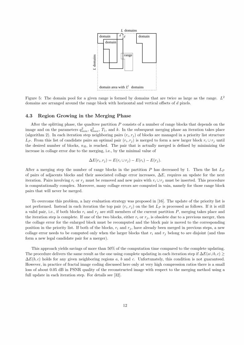
As usual, [4], we consider domain blocks that are twice as large as range blocks. In [30, 21] it has been shown,

that domains with small collage error may be found near the range block. We make use of this observation by

defining a square array of L2 domains which is centered over the corresponding range. Two neighboring domains

are offset horizontally or vertically by a fixed step size d (figure 5). Domain blocks may wrap around image

boundaries. The domain coordinates (xd, yd) in (2.1) can be encoded by an integer index id = 0, . . . , L2−1 since

the decoder can reconstruct the domain pool from a given range block.

The transform parameters s, o are quantized with the method in [5], using representations of ns and no bits,

respectively. The quantized parameters and the domain address index id are encoded using adaptive arithmetic

coding [28].

4.2 Quadtree Partitioning in the Splitting Phase

The quadtree partition proceeds along algorithm 1. We restrict the block sizes in the partition to a minimum

and maximum size, q2min and q2

max, respectively (see subsection 3.2). The split criterion is given by a threshold T

on the mean square collage error E(r)/|r| of a block r corresponding to a node of the tree. The node is expanded

and the block is subdivided into four subblocks, if E(r)/|r| > T . As in [31, 21], we use an adaptive threshold T ,

which is multiplied by a factor k for blocks of the next deeper quadtree level. For the blocks of maximum size

q2max, an initial threshold T = T1 is used.

10

0

500

1000

1500

2000

2500

3000

0 4000 8000 12000 16000

Cos

ts [b

its]

Quadtree Blocks

sum contextfull context

4 context

02000400060008000

100001200014000160001800020000

0 2000 4000 6000 8000 10000 12000

Cos

ts [b

its]

Regions

10613 quadtree blocks

REM*QBREM4QBREM3QBREM2

(a) (b)

0

2000

4000

6000

8000

10000

12000

14000

0 1000 2000 3000 4000 5000 6000 7000

Cos

ts [b

its]

Regions

6715 quadtree blocks

REM*QBREM4QBREM3QBREM2

0

2000

4000

6000

8000

10000

12000

0 500 10001500200025003000350040004500C

osts

[bits

]

Regions

4201 quadtree blocks

REM*QBREM4QBREM3QBREM2

(c) (d)

0

1000

2000

3000

4000

5000

6000

7000

8000

0 500 1000 1500 2000 2500

Cos

ts [b

its]

Regions

2449 quadtree blocks

REM*QBREM4QBREM3QBREM2

0500

1000150020002500300035004000450050005500

0 200 400 600 800 1000 1200 1400 1600

Cos

ts [b

its]

Regions

1588 quadtree blocks

REM*QBREM4QBREM3QBREM2

(e) (f)

0

2000

4000

6000

8000

10000

12000

14000

16000

0 500100015002000250030003500400045005000

Cos

ts [b

its]

Regions

6715 quadtree blocks

REM*QBREM*

fit QBREM*

0

2000

4000

6000

8000

10000

12000

0 500 1000 1500 2000 2500 3000 3500

Cos

ts [b

its]

Regions

3223 quadtree blocks

Chain CodesREM*

QBREM*

(g) (h)

Figure 4: Coding performance for quadtree-based region edge maps (QBREM) compared to plain region edgemaps (REM) for partitions of the 512×512-Lenna image based on split/merge using 4-32-quadtrees. (a) comparesthe costs of different context models for quadtree coding. (b)-(f) compare the performance of encoding QBREMsbased on quadtrees of differing complexities. (g) shows the benefits of additional quadtree fitting, and (h)compares encoding methods for QBREMs and REMs with the chain coding method in [21].

11

dd

Ldo

mai

ns

domainsL

domaindomain

domain

range

L2domain area with domains

Figure 5: The domain pool for a given range is formed by domains that are twice as large as the range. L2

domains are arranged around the range block with horizontal and vertical offsets of d pixels.

4.3 Region Growing in the Merging Phase

After the splitting phase, the quadtree partition P consists of a number of range blocks that depends on the

image and on the parameters q2min, q2

max, T1, and k. In the subsequent merging phase an iteration takes place

(algorithm 2). In each iteration step neighboring pairs (ri, rj) of blocks are managed in a priority list structure

LP . From this list of candidate pairs an optimal pair (ri, rj) is merged to form a new larger block ri ∪ rj until

the desired number of blocks, nR, is reached. The pair that is actually merged is defined by minimizing the

increase in collage error due to the merging, i.e., by the minimal value of

∆E(ri, rj) = E(ri ∪ rj) − E(ri) − E(rj).

After a merging step the number of range blocks in the partition P has decreased by 1. Then the list LP

of pairs of adjacents blocks and their associated collage error increases, ∆E, requires an update for the next

iteration. Pairs involving ri or rj must be removed and new pairs with ri ∪ rj must be inserted. This procedure

is computationally complex. Moreover, many collage errors are computed in vain, namely for those range block

pairs that will never be merged.

To overcome this problem, a lazy evaluation strategy was proposed in [16]. The update of the priority list is

not performed. Instead in each iteration the top pair (ri, rj) on the list LP is processed as follows. If it is still

a valid pair, i.e., if both blocks ri and rj are still members of the current partition P , merging takes place and

the iteration step is complete. If one of the two blocks, either ri or rj , is obsolete due to a previous merger, then

the collage error for the enlarged block must be recomputed and the block pair is moved to the corresponding

position in the priority list. If both of the blocks, ri and rj , have already been merged in previous steps, a new

collage error needs to be computed only when the larger blocks that ri and rj belong to are disjoint (and thus

form a new legal candidate pair for a merger).

This approach yields savings of more than 50% of the computation time compared to the complete updating.

The procedure delivers the same result as the one using complete updating in each iteration step if ∆E(a∪b, c) ≥

∆E(b, c) holds for any given neighboring regions a, b and c. Unfortunately, this condition is not guaranteed.

However, in practice of fractal image coding discussed here only at very high compression ratios there is a small

loss of about 0.05 dB in PSNR quality of the reconstructed image with respect to the merging method using a

full update in each iteration step. For details see [32].

12

image parameters partition costs [bits] coefficient compression PSNR

qmin, qmax T1 nR total quadtree costs [bits] ratio [dB]

Lenna 4, 32 7 2500 12727 2606 60735 28.55 33.52

5, 80 7 1140 7346 1703 27690 59.85 30.62

6, 24 45 760 5076 1206 18392 89.36 29.13

Boat 4, 32 5 2250 15686 2626 54632 29.82 30.85

4, 64 25 1115 7798 2169 27081 60.13 28.01

7, 28 15 720 5774 696 17495 90.13 26.68

Peppers 3, 24 15 2305 13382 3673 56639 29.95 33.14

4, 32 30 1160 6673 1891 28215 60.11 30.58

7, 56 25 775 4444 1148 18706 90.60 28.89

Barbara 3, 24 15 3525 21490 3793 82951 20.08 28.04

4, 32 5 2250 16586 2939 53030 30.13 26.43

4, 32 50 1120 9722 2277 26531 57.85 24.58

Table 3: Coding results for 512× 512-images Lenna, Boat, Peppers and Barbara. k = 2, L = 256, d = 2, ns = 4,no = 6.

4.4 Partition Coding

For the encoding of the quadtree-based split/merge partition P we use our quadtree-based region edge maps

as proposed in section 3. We also try the different context models from table 2 and choose the model that works

best.

5 RESULTS AND DISCUSSION

In this section we present results for the proposed fractal image coder using quadtree-based region edge

maps. For the experiments we chose the 512×512 images Lenna, Boat, Peppers, and Barbara from the Waterloo

BragZone [33]. We used the following settings for the parameters of the fractal coder introduced in the last

section.

Minimum and maximum allowed block size for the quadtree blocks ((qmin, qmax), see subsection 3.2).

For each bit rate the setting from (4, 32), (4, 64), (5, 40), (5, 80), (6, 24), (6, 48), (7, 28), (7, 56), (8, 32) that

led to the lowest distortion was selected.

Threshold and threshold factor for quadtree segmentation (T1, k, see subsection 4.2). Experiments

showed that a value of k = 2 leads to good results in most cases. However, the differences in PSNR

of the reconstructed images were very small compared to other values for k. The best value for the

threshold T1 ∈ {0, 5, . . . , 100} was determined experimentally for each bit rate.

Number of rows/columns of the domain arrays and step length (L, d, subsection 4.1). Values of L =

256 and d = 2 spread the domains uniformly over the entire image and led to best rate-distortion perfor-

mance.

Number of bits for quantization of fractal parameters (ns and no, subsection 4.1). We set ns = 4 and

no = 6. These values led to best rate-distortion performance at compression ratios larger than 30.

Number of regions in the split/merge partition (nR, subsection 4.3). The parameter varies and controls

the bit rate and the distortion.

13

2829303132333435363738

10 20 30 40 50 60 70 80 90 100

PS

NR

[dB

]

Compression ratio

Lenna

3−24 4−32 5−40 6−24 7−28 8−32

0

10000

20000

30000

40000

50000

60000

70000

80000

0 500 1000 1500 2000 2500 3000 3500 4000

Cos

ts [b

its]

Regions

Lenna

coefficientsREM

QBREM

(a) (b)

2829303132333435363738

10 20 30 40 50 60 70 80 90 100

PS

NR

[dB

]

Compression ratio

Lenna

QBREMREM

quadtree only (rd optimized)

25262728293031323334353637

10 20 30 40 50 60 70 80 90 100

PS

NR

[dB

]

Compression ratio

Boat

QBREMREM

quadtree only (rd optimized)

(c) (d)

2728293031323334353637

10 20 30 40 50 60 70 80 90 100

PS

NR

[dB

]

Compression ratio

Peppers

QBREMREM

quadtree only (rd optimized)

23

24

25

26

27

28

29

30

31

32

10 20 30 40 50 60 70 80 90 100

PS

NR

[dB

]

Compression ratio

Barbara

QBREMREM

quadtree only (rd optimized)

(e) (f)

Figure 6: (a) Comparison of different base block sizes for region merging (Lenna); (b) costs for fractal coefficientsand domain addresses compared to partition coding costs for REM and QBREM (Lenna); (c-f) rate-distortionperformance for four test images: quadtree-based split/merge approach versus merging of blocks from a uniformpartition and fractal encoding with rate-distortion optimized quadtree (without block merging).

14

Figure 6 summarizes the results of our experiments. In part (a) we show that the choice of the minimal

and maximal block sizes in the quadtree partition that provides the base blocks for the merging phase is crucial

for the rate-distortion performance of the fractal codec. Especially for low compression ratios (below 40) we

observed that a small minimal block size of 3× 3 pixels provided much better results than larger sizes. For high

compression ratios (above 80) larger blocks sizes gave better PSNR performance, however, only by a very small

amount.

Part (b) of figure 6 displays how much of the bit rate was spent on the adaptive split/merge partition in

comparison to the rest of the code consisting of domain addresses and coefficients. It also demonstrates the

advantage of our coding scheme exploiting the underlying quadtree structure opposed to encoding plain region

edge maps. The difference was as large as about 2000 bits for medium compression ratios.

Parts (c-f) of figure 6 shows complete rate-distortion curves of our fractal coder with quadtree-based region

edge maps, with plain region edge maps, and with a quadtree partition without subsequent block merging. Each

of the plots is for one of the four test images. The plain quadtree coder is superior to that of Fisher [5]. We

implemented a rate-distortion optimization that is guaranteed to select the subtree of the complete quadtree that

yields minimum collage error using optimization methods given in [34, 35]. Moreover, for the quadtree encoding

we used arithmetic coding with context modelling as proposed in this paper. Our results indicate that fractal

coders that use an adaptive split/merge image partition may outperform optimized fractal quadtree coders by

about 0.5 to 1 dB in PSNR. Using a quadtree as a base partition in the split/merge partitions provided gains of

about 0.2 dB in PSNR. Table 3 lists detailed numerical coding results obtained with the proposed method.

In figures 7 and 8 we present reconstructions of encoded Lenna and Peppers images at compression ratios

about 70. Parts (a) show the original image for reference, parts (b) show the reconstructed images (detailed

parameters are given in the captions). Parts (c) show images decoded from JPEG2000 encoded originals. For

the JPEG2000 encodings we used the kakadu encoder [36]. Parts (d) and (e) show the inverted difference images

between decoded and original images. The difference images were obtained from the absolute differences between

grey values of corresponding pixels, scaled by a factor of 5 and clamped at 255. The rate distortion performance

of our coder is comparable to that of the JPEG2000 coder with an advantage of JPEG2000 of about 0.3 to 0.5 dB

PSNR. The decoded images and the difference images, however, show much more noticeable differences in terms

of typical artifacts. While the images obtained from JPEG2000 codes look defocussed especially around edges,

here the fractally decoded images clearly have sharper edges. This impression is confirmed by the difference

images which show broader edge artifacts for the wavelet coded images of JPEG2000. On the other hand

there are blocking artifacts in smooth image regions of the fractally decoded images. We remark that there are

postprocessing techniques that may improve the sharpness of the JPEG2000 reconstructions [37] and reduce the

blocking artifacts of fractally encoded images [38, 21].

Finally, in figure 9 we display quadtree partitions for two test images that provided the base blocks for the

merging phase. The resulting adaptive split/merge partitions are also shown.

The survey in [6] showed a comparison of the performance of published pure fractal coding methods that

are working in the spatial domain ([6, figure 6]). This comparison includes methods based on various types of

adaptive image partitions, such as quadtrees [5], HV-partitions [5], Delaunay-triangulations [11, 12], and irregular

partitions [14, 15, 20]. The rate-distortion performance of our coder is clearly superior to all of these.

Fractal image coding with quadtree-based split/merge partitions was first proposed in [20, 21], where the

chain coding method of [25] was adapted. Our reimplementation of the chain coder showed that our QBREM

coding algorithm compressed partitions with only half the rate, see figure 4h.

15

(a)

(b) (c)

(d) (e)

Figure 7: Coding example for 512×512–image Lenna with parameters qmin = 6, qmax=48, T1 = 15, k = 2,L = 256, d = 2, ns = 4, no = 6 and nR = 990. (a) Original image; (b) decoded image with proposedfractal coder, PSNR = 30.00 dB, compression ratio = 70.29; (c) decoded image from encoding with JPEG2000(kakadu encoder), PSNR = 30.40 dB, compression ratio = 71.02; (d) difference between fractal reconstructionand original; (e) difference between JPEG2000 reconstruction and original.

16

(a)

(b) (c)

(d) (e)

Figure 8: Coding example for 512×512–Peppers with parameters qmin = 4, qmax = 32, T1 = 40, k = 2,L = 256, d = 2, ns = 4, no = 6 and nR = 990. (a) Original image; (b) decoded image with proposed fractalimage coder, PSNR = 29.91 dB, compression ratio = 70.30; (e) decoded image from encoding with JPEG2000(kakadu encoder), PSNR = 30.24 dB, compression ratio = 69.46; (d) difference between fractal reconstructionand original; (e) difference between JPEG2000 reconstruction and original.

17

(a) (b)

(c) (d)

Figure 9: Partitions for the encodings in figures 7 and 8. (a) Lenna image, quadtree partition with 1345 blocksbefore merging; (b) partition with 990 regions after merging quadtree blocks; (c) Peppers, quadtree partitionwith 1698 blocks before merging; (d) partition with 990 regions after merging quadtree blocks.

6 CONCLUSIONS

We proposed a fractal image compression method based on split/merge image partitions. In the splitting

phase an image adaptive quadtree partition is generated. Neighboring blocks are iteratively merged using an

appropriate error criterion. We provided an algorithm for lossless arithmetic compression of the resulting image

partition with suitable context modelling that exploits the structure of the underlying quadtree. Experimental

results show that our method can save up to 30% of the total rate for the partition in comparison to encoding

with region edge maps based on uniform base partitions. When applied to fractal image coding we obtained rate-

distortion performances that exceed the best known results for pure, non-hybrid fractal image coders. Compared

to state of the art wavelet coders in industry, given by the JPEG2000 standard, our fractal compression method

is comparable in terms of rate-distortion performance up to less than 0.5 dB PSNR. Subjectively, fractally

reconstructed images have sharper edges and more contrast than JPEG2000 reconstructions but suffer from mild

blocking artifacts.

Our coding method for quadtree-based region edge maps can also be used in connection with other image

18

coding systems that rely on adaptive partitions. For example, similar partitions have been used with dynamic

coding [39], or one may modify the segmentation-based image coding method in [40] to make use of quadtree-

based split/merge partitions.

ACKNOWLEDGMENT

This work was supported by grant Sa449/8-2 of the Deutsche Forschungsgemeinschaft.

19

REFERENCES

[1] M. F. Barnsley, A. D. Sloan, ”Chaotic compression”, Computer Graphics World, 1987.

[2] M. F. Barnsley, A. D. Sloan, ”A better way to compress images”, Byte, 1988, pp. 215–223.

[3] A. E. Jacquin, ”A fractal theory of iterated markov operators with application to digital image coding”, Ph.D.

Dissertation, Georgia Institute of Technology, 1989.

[4] A. E. Jacquin, ”Image coding based on fractal theory of iterated contractive image transformations”, IEEE

Transactions on Image Processing, 1(1) (1992), pp. 18–30.

[5] Y. Fisher, ”Fractal Image Compression – Theory and Application”, Springer Verlag, New York, 1995.

[6] B. Wohlberg, G. de Jager, ”A review of the fractal image coding literature”, IEEE Transactions on Image

Processing, 8(12) (1999), pp. 1716–1729.

[7] D. Saupe, R. Hamzaoui, A. Zerbst, ”The Paper Collection on Fractal Image Compression”,http://www.inf.uni-konstanz.de/cgip/fractal/papers.html

[8] Y. Fisher, S. Menlove, ”Fractal encoding with HV partitions”, in Fractal Image Compression – Theory andApplication, pp. 119-126. Springer-Verlag, 1995.

[9] D. Saupe, M. Ruhl, R. Hamzaoui, L. Grandi, D. Marini, ”Optimal hierarchical partitions for fractal image com-pression”, Proceedings IEEE International Conference on Image Processing, 1998.

[10] E. Reusens, ”Partitioning complexity issue for iterated function systems based image coding”, Proceedings VIIth

European Signal Processing Conference, I (1994), pp. 171–174.

[11] F. Davoine, J.-M. Chassery, ”Adaptive Delaunay triangulation for attractor image coding”, Proceedings 12th

International Conference on Pattern Recognition, 1994, pp. 801–803.

[12] F. Davoine, J. Svensson J.-M. Chassery, ”A mixed triangular and quadrilateral partition for fractal image coding”,Proceedings IEEE International Conference on Image Processing, 1995.

[13] R. C. Gonzales, R. E. Woods, ”Digital Image Processing”, Addison-Wesley, Reading, Massachusetts, 1993.

[14] L. Thomas, F. Deravi, ”Region-based fractal image compression using heuristic search”, IEEE Transactions on

Image Processing, 4(6) (1995), pp. 832–838.

[15] M. Ruhl, H. Hartenstein, D. Saupe, ”Adaptive partitionings for fractal image compression”, Proceedings IEEE

International Conference on Image Processing, 1997.

[16] H. Hartenstein, M. Ruhl, D. Saupe, ”Region-based fractal image compression”, IEEE Transactions on Image

Processing, 9(7) (2000), pp. 1171–1184.

[17] H. Freeman, ”On the encoding of arbitrary geometric configurations”, IRE Transactions on Electronic Computers,EC-10 (1961), pp. 260–268.

[18] S. R. Tate, ”Lossless compression of region edge maps”, Technical Report DUKE–TR–1992–09, Duke University,

Durham, 1992.

[19] S. L. Horowitz, T. Pavlidis, ”Picture segmentation by a tree traversal”, Journal of the ACM, 23 (2) (1976), pp.368–388.

[20] Y. C. Chang, B. K. Shyu, J. S. Wang, ”Region-based fractal image compression with quadtree segmentation”,Proceedings IEEE International Conference on Acoustics, Speech and Signal Processing, 4 (1997), pp. 3125–3128.

[21] Y. C. Chang, B. K. Shyu, J. S. Wang, ”Region-based fractal compression for still image”, Proceedings 8-th

Internations Conference in Central Europe on Computer Graphics, Visualization and Interactive Digital Media,2000.

[22] M. Barnsley, ”Fractals Everywhere”, Academic Press, San Diego, 1988.

[23] M. Barnsley, L. Hurd, ”Fractal Image Compression”, AK Peters Ltd, 1993.

[24] M. Eden, M. Kocher, ”On the performance of a contour coding algorithm in the context of image coding. Part I:contour segment coding”, Proceedings IEEE Internations Conference on Acoustics, Speech and Signal Processing,8 (1985), pp. 381–386.

[25] T. Ebrahimi, ”A new technique for motion field segmentation and coding for very low bitrate video coding appli-cations”, Proceedings IEEE International Conference on Image Processing, 2 (1994), pp. 433–437.

[26] D. Saupe, M. Ruhl, ”Evolutionary fractal image compression”, Proceedings IEEE International Conference on

Image Processing, 1996.

[27] G. G. Langdon, J., Rissanen, ”Compression of black-white images with arithmetic coding”, IEEE Transactions on

Communications, 29(6) (1981), pp. 858–867.

20

[28] I. H. Witten, R. M. Neal, J. G. Cleary, ”Arithmetic coding for data compression”, Communications of the ACM,30(6) (1987), pp. 520–540.

[29] H. Samet, ”The quadtree and related hierarchical data structure”, ACM Computing Surveys, 16(2) (1984), pp.187–260.

[30] K. U. Barthel, T. Voye, P. Woll, ”Improved Fractal Image Coding”, Proceedings International Picture Coding

Symposium, 1993.

[31] E. Shusterman, M. Feder, ”Image compression via improved quadtree decomposition algorithms”, IEEE Transac-

tions on Image Processing, 3(2) (1994), pp. 207–215.

[32] T. Ochotta, ”Regionenbasierte Partitionierung bei fraktaler Bildkompression mit Quadtrees”, Diplomarbeit, Institut

fur Informatik, Universitat Leipzig, Germany, 2002.

[33] J. Kominek, ”Waterloo BragZone”, University of Waterloo, Canada, http://www.uwaterloo.ca/bragzone.base.html.

[34] G. Sullivan, R. Baker, ”Efficient quadtree coding of images and video”, IEEE Transactions on Image Processing,3(3) (1994), pp. 327–331.

[35] R. Hamzaoui, D. Saupe, ”Combining fractal image compression and vector quantization”, IEEE Transactions on

Image Processing, 9(2) (2000), pp. 197–208.

[36] D. Taubman, ”The sporty new JPEG model”, SPIE’s oemagazine, 2002, pp. 38–40.kakadu software http://www.kakadusoftware.com

[37] G. Fan, W. K. Cham, ”Post-processing of low bit-rate wavelet-based image coding using multiscale edge character-ization”, IEEE Transactions on Circuits and Systems for Video Technology, 11(12) (2001), pp. 1263–1272.

[38] K. G. Nguyen, D. Saupe, ”Adaptive postprocessing for fractal image compression”, Proceedings IEEE International

Conference on Image Processing, 2000.

[39] E. Reusens, T. Ebrahimi, C. Le Buhan, R. Castagno, V. Vaerman, L. Piron, C. de Sola Fabregas, S. Bhattacharjee,F. Bossen, M. Kunt, ”Dynamic approach to visual data compression”, IEEE Transactions on Circuits and Systems

for Video Technology, 7(1) (1997), pp. 197–211.

[40] X. Wu, ”Image coding by adaptive tree-structured segmentation”, IEEE Transactions on Information Theory,38(6) (1992), pp. 1755–1767.

21