Edge Detection by Multi-Dimensional Wavelets

Marlana Anderson∗, Chris Brasfield†, Pierre Gremaud‡,Demetrio Labate§, Katherine Maschmeyer¶,

Kevin McGoff‖, Julie Siloti∗∗

August 1, 2007

Abstract

It is well known that one-dimensional wavelet techniques are suboptimal in therepresentation of images. Recently a new generation of intrinsically two-dimensionalwavelets, e.g. shearlets, has been introduced to alleviate these deficiencies. In thisproject, new edge detection methods were developed based on the shearlet transform.As a refinement of these methods, subdomain decomposition was introduced to preserveless dominant edges. Furthermore, several basic post-processing schemes were used toprovide more distinct edges. All of the above methods were applied to both artificiallygenerated and natural images. In order to measure the accuracy of the various methods,the Hausdorff distance between the actual and approximate edges of artificial imageswas computed. Through this analysis, it was concluded that edge detection methodsbased on shearlets are at least as accurate as popular methods, such as Canny andSobel. On images with sharp corners, the results suggest that shearlet methods mayactually improve upon traditional methods.

1 Introduction

Wavelets are collections of functions that can be used to decompose signals into variousfrequency components at an appropriate resolution for a range of spatial scales. Edges canbe defined as sharp changes of the intensity in a signal. Since wavelets provide excellentrepresentations of discontinuous signals [8], they have been used in modern edge detection

∗Albany State University, REU Group Member†North Carolina State University, Graduate Assistant‡North Carolina State University, Project Mentor§North Carolina State University, Consultant¶Washington University in St. Louis, REU Group Member‖University of Maryland, REG Group Member∗∗Pomona College, REU Group Member

1

methods [11, 12]. Applications of edge detection technology can be found in many fields,including medical imaging. The objective of this project was to explore the latest generationof wavelets in order to create improved edge detectors.

Toward this end, several known signal-processing methods were studied and applied.These included methods based on the well-known Fourier transform and wavelet transformsin both one and two dimensions. Theoretical results concerning edge detection in one di-mension were reviewed and the corresponding algorithms were implemented. Furthermore,tests were run on images by applying one-dimensional decompositions in both the horizon-tal and vertical directions independently. These results were compared to edge detectionschemes based on gradient methods, which seek to capture sharp changes in intensity byapproximating the gradient in the neighborhood of each pixel.

It is well known that one-dimensional wavelet techniques are suboptimal in the repre-sentation of images [8]. Recently a new generation of intrinsically two-dimensional wavelets,e.g. shearlets [8], has been introduced to alleviate these deficiencies. In this project, newedge detection methods were developed based on the shearlet transform. As a refinement ofthese methods, subdomain decomposition was introduced to preserve less dominant edges.Furthermore, several basic post-processing schemes were used to provide more distinct edges.All of the above methods were applied to both artificially generated and natural images. Inorder to measure the accuracy of the various methods, the Hausdorff distance between theactual and approximate edges of artificial images was computed.

Section 2 recalls the necessary background information, including a construction ofwavelets and shearlets, as well as a description of various previous edge detection meth-ods. For more information on wavelets, see [3, 4, 5, 10, 19, 20]. For a detailed discussion ofshearlets, see [8].

Section 3 contains a description of the new edge detection algorithm using shearlets,including a discussion of the theory, implementation, and results of this new method.

2 Background Information

2.1 Wavelets

The purpose of wavelets is to provide a decomposition of a function or signal into its variousfrequency components and at a range of appropriate spatial scales, or resolutions. For agiven function f , wavelets give a collection of functions {ψjk} such that f can be representedas the superposition of some linear combination of ψjk. Such a collection is often called awavelet basis. More precisely, for a given f , there exist coefficients cjk such that for all x,

f(x) =∑j,k

cjkψjk(x). (1)

We say that a single term in the sum, cjkψjk, is the frequency component of f at a certainspatial scale and position. Thus, Equation (1) can be viewed as the decomposition of f intoits various frequency components at a range of scales.

2

To understand how, exactly, wavelets yield such a decomposition, more definitions arerequired. First, consider a function φ, which is normalized, i.e.∫ ∞

−∞φ(x)dx = 1,

and which satisfies the Dilation Equation for some coefficients ak:

φ(x) =∑k

akφ(2x− k). (2)

Such a φ will be called a “scaling function.” From this function we can define another functionψ as follows:

ψ(x) =∑k

(−1)ka1−kφ(2x− k). (3)

Such a ψ will be called a “mother wavelet,” because it is used to generate the entire collection{ψjk}. A wide variety of functions meet these criteria. For example, the Daubechies 4 wavelet(see Fig. 1, created by [19]) can be obtained by choosing coefficients 1

4(1 +

√3), 1

4(3 +

√3),

14(3 −

√3), 1

4(1 −

√3), and this yields a nowhere differentiable function with a fractal-like

structure [3, 4, 5, 19]. On the other hand, it can be shown that the derivative of a Gaussianfunction satisfies the above conditions (with an infinite number of coefficients), [17], andthese wavelets are smooth.

WAVELETS AND DILATION EQUATIONS 619

(1, I, 1, 1) is a left eigenvector with X = I. The right eigenvector yields the values $( I ) , . . .,$ (N )at the integers. The recursion determines $ at all dyadic points. Values at other points are never used.

1.2. Wavelets and orthogonality. Finally we define a wavelet. It comes from the scaling function $ by taking "differences":

We write Win place of the usual rl/, to distinguish more clearly from $. Note the 2x on the right, and especially (- l)k. Examples show the effect of alternating signs:

Haar wavelet from box function Wavelet from hat function

W,(x)=$(2x)-$(2x- I) ~=$(2x) -$$(2x- 1)-$$(2x+ 1)

W4(x) from $ = D4 Orthogonal wavelet

The wavelet from the hat function does not belong here. It is not orthogonal to W(x + 1). The point is that the other two do belong. The Haar function is orthogonal to its own translations and dilations. Historically it was the original wavelet (but with p = 1 and poor approximation). The orthogonal wavelet W4 has p = 2 and second- order approximation.

Without formulas for D4 and W4, how is the orthogonality of their translates known? We need a test that applies to the recursion coefficients ck, or to the symbol P([)= $ 2 ckelk(.

Figure 1: The Daubechies 4 wavelet

Now, given a mother wavelet ψ, we define the wavelet basis by dilations and translations:

ψjk(x) = 2j/2ψ(2jx− k).

3

Note that in this case the coefficients in Equation (1) are in fact given by

cjk =< f, ψjk >, (4)

where <,> is the inner product on L2(R).The idea of decomposing a signal into frequency components has been heavily exploited

with the use of Fourier decompositions, which use sines and cosines as their basis functions.The clear advantage of wavelets over traditional Fourier methods is that they are very well-localized in both space (or time) and frequency. Recall that trigonometric functions capturefrequencies perfectly, but they are truly global in the sense that they do not decay overtime. Thus, these types of bases give poor representations of functions that have short“blips,” or any discontinuities. On the other hand, wavelet bases can be constructed so thatthey capture only local information in both space and frequency domains, and thereforewavelets provide a much better representation of discontinuous or non-periodic functions.Furthermore, this locality property in the space domain allows for so-called multi-resolutionanalysis [14], which simply means that frequency information is captured for a full range ofscales (indexed by j in Equation 4).

The same process can be carried out for functions of two variables, except that the theoryrequires use of three mother wavelets, ψ1, ψ2, and ψ3, which are called ‘horizontal,’ ‘vertical,’and ‘diagonal,’ respectively. The wavelet basis then has three indices:

ψijk(x) = 2j/2ψi(2jx− k), (5)

where k is now an element of Z2.

2.2 Shearlets

While one-dimensional wavelets provide optimal representation of discontinous signals in onedimension (a statement that will not be made precise in this paper), the two-dimensionalwavelets described above provide provably suboptimal representation of two-dimensionalsignals [8]. For this reason, a wide variety of alternative approaches to two-dimensionalsignal decompositions have appeared in recent years, notably bandlets [13], contourlets [7],ridgelets [1], curvelets [18], and shearlets [8]. Each of these approaches attempts to takeadvantage of some two-dimensional geometric information to provide better representation.These approaches can provide better representation properties, but usually at some cost.For example, shearlets provide provably optimal representations of signals, but at the costof orthogonality of the basis functions [8]. The shearlet decomposition functions form aParseval frame, but not a true basis. Recall that a Parseval frame for L2(R2) is a collectionof functions {ψj} such that for any f in L2(R2),

||f ||2 =∑j

| < f, ψj > |2

Considering Parseval frames instead of bases is typically not a large disadvantage, since theonly difference is that Parseval frames contain a certain amount of redundancy. In this paperwe focus our attention on shearlets.

4

Constructing shearlet bases is a non-trivial task, but it will be presented here nonetheless.First, let ψ be a “mother shearlet,” which has certain technical properties (as defined in [8]).Then define the matrices Aj, which is the dilation matrix, and Bl, which is the shear matrix,as:

Aj =

(2j 00 2j/2

),

and

Bl =

(1 l0 1

).

Now we can define shearlets to be the functions

ψjkl = | detA|j/2ψ(BlAjx− k), (6)

where j, l are in Z and k is in Z2. With this definition, shearlets will be well-localized inboth space and frequency domains. The shearlet ψjkl is supported in frequency domain ontrapezoids at scale 2j, with orientation indexed by l, and associated with spatial locationindexed by the vector k. Thus shearlets provide a decomposition of any L2(R2) function intoits frequency components according to the tiling of frequency domain by such trapezoids(see Fig. 2, created by the authors of [8]).

The support of a shearlet in space domain is highly-localized; moreover, the support alsomaintains a specific orientation (loosely orthogonal to the line along which the correspondingtrapezoids lie in frequency domain). This additional information constitutes the entire goalof shearlets: certain two-dimensional geometric information about the signal–such as theorientation–can be used to provide more efficient representation of the signal.

2.3 Edge Detection

As mentioned in the introduction, edge detection has a wide variety of important appli-cations. For this reason, it has been studied quite extensively, both theoretically and nu-merically. Theoretically, the edges can be defined (for piecewise smooth pictures, wherethe discontinuities occur only along smooth curves) as the collection of points at which thegradient is infinite.

The idea of considering large gradients leads to various methods for edge detection in thediscrete case. All of these methods define some discrete differential operator that approxi-mates the gradient in some way. For example, the Sobel method [15] uses convolution withthe following matrix to approximate the partial derivative in the horizontal direction:

Dx =

1 0 −12 0 −21 0 −1

.

Recall that the discrete convolution product of two matrices A and B is given by:

(A ∗B)ij =∑k

∑l

ak,lbi−k,j−l. (7)

5

Alternative tiling of the frequency plane induced by the shearlets:we tile the cone |!2/!1| ! 1, next we tile the cone |!2/!1| > 1.

43Figure 2: Tiling of Frequency Domain induced by Shearlets

Once this operator has been applied to the signal at each point in the image, the pointsat which the gradient is ‘large’ must be determined, and these points are then labeled asthe edges. Gradient methods work quite well for truly smooth images, but they are highlysusceptible to the effects of noise.

In order to reduce the effects of noise, other methods have been explored, such as thespectral methods seen in [9] and the wavelet methods in [11, 12]. These methods work verywell in one dimension, but in order to extend them to two dimensional signals, the onedimensional methods are applied twice (once in the horizontal direction and once in thevertical direction) and then combined. Due to this seemingly naive method of extension,these methods do not take into account the truly two dimensional information of edges.

The fundamental idea for the spectral methods in one dimension is to note that theconjugate Fourier sum of a discontinuous function f (of one variable), SNf , converges to thefunction [f ](x) = f(x+) − f(x−), which is only non-zero at the discontinuities, as N goesto ∞. In the proposed versions of this method, the authors have generalized the conjugateFourier sum so that the convergence to [f ] will actually be exponential. These methodsdo decrease the effects of noise, but they are still susceptible to spurious oscillations near

6

the discontinuities, which leads the authors to use a combination of gradient and Fouriermethods.

The one dimensional wavelet methods introduced in [11, 12] rely on convoluting the signalwith a smooth wavelet function. Recall that the convolution product of functions f and ψis given by

f ∗ ψ(x) =

∫ ∞−∞

f(t)ψ(t− x)dt

Notice that if the wavelet ψ is the derivative of a smoothing function (like a Gaussian) φ, thenthe convolution of a signal f with ψ is equivalent to taking the derivative of the convolutionof the f with φ:

(f ∗ φ)′ = f ∗ φ′ = f ∗ ψ, (8)

by the properties of the convolution product. Therefore the one-dimensional edge detectionmethods are theoretically equivalent to smoothing the signal, taking the derivative, andlooking for large values of the derivative. They remain advantageous, though, because inpractice they are fast and the smoothing reduces the effects of noise. Also, since the waveletcoefficients are localized in space and frequency domains, there are no spurious oscillationswith which to contend. Given a function f , the first step is to compute the wavelet transform,

Wf(s, x) = f ∗ ψs(x), (9)

where ψs(x) = 1sψ(x

s). Note that this just gives the coefficients of the wavelet decomposition

in the case that we choose s = 2j. Next we define a modulus maxima of Wf(s, x) at a fixedscale s to be a local maxima of |Wf(s, x)|, viewed as a function of x. The main theorem in[11, 12] then states that under certain conditions on ψ (such as having at least one vanishingmoment and being the derivative of a smoothing function), the set of discontinuities of f iscontained in the closure of the set of modulus maxima of Wf(s, x). In practical terms, thistheorem implies that finding the modulus maxima of Wf(s, x) as s→ 0 should detect all ofthe edges of a function f (although it may detect more points, in general). In other words,we obtain an edge detector in the discrete case by simply looking at fine scales and findingthe local maxima of |Wf(s, x)| as a function of x. This method can be observed clearly bylooking at the absolute value of these coefficients, as seen in Fig. 3, which was created usingthe Gaussian wavelet.

The wavelet methods mentioned above have been applied to two dimensional images withsome success, but since the method of extension from one to two dimensions seems not totake into account any truly two dimensional information, it appears that there is room forimprovement.

3 Edge Detection with Shearlets

3.1 Theory

The goal of the present work is to show that the newest generation of two-dimensionalwavelets can yield viable edge detectors. To the best of the authors’ knowledge, the literature

7

Figure 3: Local maxima converge to the discontinuities

currently contains no edge detection method based on any of these representations. Not onlyare there no theoretical results regarding the effectiveness of such methods, there are also nonumerical results suggesting that such methods may work.

According to preliminary studies, there may be a strong analogy between the methodsfound in [11, 12] and the methods attempted here. Such an analogy suggests that similartheoretical results may be achieved, although this remains a topic of continuing research.All known results do suggest that such methods may be fruitful. Indeed, shearlets provideprovably optimal representation of two dimensional images by incorporating two dimensionalgeometrical information into a multiscale decomposition. Moreover, this additional geometricinformation pertains to the orientation of the signal at a particular point, and this type ofinformation is precisely what the prior edge detection methods appear to be missing.

8

3.2 Implementation

The idea for a shearlet edge detector has been inspired by the analogy to the wavelet methoddetailed in [11], and therefore the algorithm is also analogous to the wavelet method describedin Section 2.3. Here we describe the algorithm used in this study. All numerical computa-tions were done using MATLAB.

The algorithm is organized as follows:

1. Gaussian smoothing: Reduce the effects of noise by convoluting the image with a Gaussianfilter.

2. Calculate shearlet coefficients for 2n distinct directions, where n is the level of detail.

3. Detect modulus maxima and thus edges using subdomain decomposition and thresholding.

4. Combine information from the 2n directions: Flag points where at least one of the sets ofdirectional coefficients detects an edge.

5. Neighborhood cleanup: Keep edges only at points where the magnitude of the neighboringdifference is greater than the magnitude of the directional coefficients. Also, keep edgesonly at points where the magnitude of the the directional coefficients is greater than thethresholding parameter.

6. Post processing: further refine the image with techniques such as line thinning and deletionof isolated points.

Each step of the algorithm is explained in further detail below.

Gaussian Smoothing

First, the image must be smoothed to reduce the effects of noise. This is done by con-voluting the rows of the image with a 1D Gaussian filter as discussed previously, therebycreating a new image, and then convoluting the columns of the new image with the 1DGaussian filter. This achieves the effect of convoluting the image with a 2D Gaussian filterbecause the Gaussian filter is separable.

Calculate Shearlet Coefficients

The next step of the algorithm is to compute the coefficients of the discrete shearlet trans-form at the jth level of detail, which can be done with a fast algorithm for images of size2n× 2n. The algorithm for computing this transform comes from work by the authors of [8].The result of this computation is 2j coefficient arrays (each of which has the same size asthe original image), where j is the level of detail, i.e. the index of the scale in the notationof Section 2.2, and each array contains the shearlet coefficients at this level of detail with a

9

single orientation. In other words, at the scale 2j, there are 2j distinct orientations for whichwe compute the shearlet coefficients, and these are collected in arrays corresponding to theorientations.

Thresholding

At various points in the algorithm, it makes sense to ignore very small effects and con-sider only the dominant effects. This is a very general concept, which is present in any edgedetector and is often called thresholding. If M = (mi,j) is any two-dimensional array, thenthe transformation “threshold M with parameter ε” is given by

(TεM)i,j =

{mi,j if |mi,j| ≥ ε

0 if |mi,j| < ε.

For example, given an array of intensity values ranging from 0 to 256, it will not alter thepicture in any significant way if those pixels with intensity values less than three are set tozero. Of course, this concept can be applied at multiple stages in an algorithm: any timewhen relatively small values should be set to zero. From a certain perspective, thresholdingis necessary, because every pixel must be labeled as either lying on an edge or not lying onan edge, and somewhere a line must be drawn to distinguish the two. Furthermore, thresh-olding helps reduce the effects of noise, since often the features introduced to an image bynoise are dominated by the actual features of the image.

Detect Modulus Maxima

The third step in the algorithm is to take the absolute values of the coefficients and find thelocal maxima. Note that in the one-dimensional case there is only one direction of approachfor a given point in space, and thus the property

P1: x is a local maximum

is the same as the property

P2: x is a local maximum along some line passing through x.

This fact no longer holds in two dimensions. In two dimensions, P1 holds when x is apoint discontinuity, whereas P2 holds when x is likely to be part of an edge. Thus, for thepurposes of edge detection, the proper extension of ‘x is a local maximum’ is actually P2.Thus, the algorithm looks for local maxima in the shearlet coefficient arrays along eight di-rections: lines making angles kπ

8with the horizontal, for k = 0, . . . , 7. The purpose of looking

for maxima along eight directions is to capture the additional directional information givenby shearlets. In fact, through direct comparison of methods, the edge detector that found

10

maxima in eight directions proved itself to be more robust with respect to the thresholdingparameter than the edge detector that found maxima in only four directions (along linesmaking angles kπ

4with the horizontal, for k = 0, . . . , 3), as shown in Figure 5.

At this step there is also a certain relative thresholding that occurs, which is based ona method that decomposes the data into smaller subdomains, also known as subdomain de-composition. In this approach, each set of shearlet coefficients (for a given orientation andlevel of detail) is divided into four basic quadrants. The local maximum for each quadrantis determined and the largest of such maxima is flagged and recorded as the new maximumfor its corresponding quadrant. The other local maxima are flagged as local maxima fortheir respective quadrants if and only if they are greater than a given fraction amount of thislargest maximum. Otherwise, the largest local maximum is flagged as the local maximumfor that entire quadrant. This process is applied recursively to each quadrant of the sub-division until either the local maximum is not sufficiently large (i.e. the largest maximumof the subdivision is used for the entire region of interest) or the size of the subdivision issmaller than a given minimum pixel size. This produces a matrix of values that indicatethe local maximum to be used for each pixel of the image. The thresholding that followseliminates extraneous local maxima by dictating that if the magnitude of the coefficient isless than that of its neighbor by a fractional amount of the corresponding local maximum,then it is not an edge. In other words, subdomain decomposition allows for local maxima tobe determined based on truly local information. In particular, consider an image with highintensity edges in one region and low intensity edges in another. If the low intensity region issufficiently close in magnitude to the high intensity region, then subdomain decompositionallows for the use of smaller threshold values for the low intensity region. As a result, morelow intensity maxima will be detected, while still ruling out extraneous maxima which mayoccur due to noise or numerical error.

Combine Information

In the next step, the magnitude of the shearlet coefficients is reincorporated at each point.To be exact, each point that has been flagged as a local maxima in at least one of the coef-ficient arrays is then multiplied by the absolute value of the associated shearlet coefficient,and the arrays are added together (pointwise). (As an interesting note, points which havebeen flagged as edges in multiple directions may contain further geometric information, suchas information about corners, but this has not been confirmed.) Then this array is onceagain thresholded to keep only the dominant edge candidates.

Neighborhood Cleanup

At this stage in the algorithm, the neighborhoods of actual edges (especially near corners)contain too many edge candidates. In order to eliminate these effects, a cleanup algorithmis implemented. Given the original image U = (ui,j), first define the difference coefficients

11

D = (di,j) to be

di,j = max(|ui,j − ui+1,j|, |ui,j − ui,j+1|).Then, given the coefficient array M = (mi,j) defined in the previous step of the algorithm,form the matrix N by the formula

(N)i,j =

{mi,j if |mi,j| < |di,j|

0 if |mi,j| ≥ |di,j|.

After doing this type of cleanup, the second instance of thresholding occurs. In otherwords, the transformation Tε (defined above) is applied to the array N . As always, thresh-olding relies on the parameter ε. There is a default value for the parameter, which givesminimal error on artificial images (see Section 3.3), although the parameter can be manuallyvaried if necessary. It is interesting to note that the error on artificial images does indeedattain a minimum, and this minimum error seems to be fairly robust with respect to changesin the parameter. Figure 7 illustrates this concept. In general, a very low threshold allowstoo much noise to be labeled as edges, and a very high threshold will cause the actual edgesto be lost. Sometimes there is a satisfactory parameter value that balances these concerns,but if the noise is too large (relative to the actual edges), then it may be difficult to findan appropriate parameter value. This phenomenon occurs in some form in any known edgedetector. At the end of this step in the algorithm, any non-zero element in the array N isset to the value 1.

Post Processing

Finally, the algorithm performs some elementary post-processing techniques. The first ofthese techniques involves deleting points which have no other points in their immediateneighborhood. The second technique is called line thinning in the literature, and it attemptsto delete extraneous points hanging off the edge of a clear line. For example, suppose thatthe matrix M represents the edges of a signal, as computed above:

M =

0 0 0 0 00 0 0 0 00 0 1 0 01 1 1 1 10 0 0 0 0

.

Then line thinning would remove the central pixel.

3.3 Testing and Results

Through rigorous testing, the shearlet edge detection method has been shown to be verycompetitive in detecting the edges of both artificial and natural images. The artificial imageshave been created using analytical formulas in such a way that the actual edges are known.

12

For these images, the known edges are compared to the approximate edges (as detected bythe shearlet method) using the familiar notion of the Hausdorff distance between two sets inR2, i.e. if A and B are two sets of points in R2, then the Hausdorff distance between A andB is computed as follows. For each a in A, let

dist(a,B) = minb∈B||a− b||.

Then the distance from A to B (which may not be the distance from B to A) is given by

dist(A,B) = maxa∈A

dist(a,B).

The Hausdorff distance between A and B is then given by

H(A,B) = max{dist(A,B), dist(B,A)}.

Note that with these definitions, dist(A,B) 6= dist(B,A) in general, but H(A,B) = H(B,A).This metric gives a precise method for measuring the effectiveness of an edge detector when-ever the edges are known.

For all artificial images tested so far, where the edges E are known, the shearlet methodsintroduced in this paper consistently yield edges F such that H(E,F ) = 1. An error ofH = 1 indicates that given any pixel in the approximate edges, it is at most one pixel awayfrom the true edges, and vice versa. The artificial images tested so far include regular n-gons with n = 3, . . . , 10 and n = 1000, as well as the irregular polygon seen in Figure 8.Traditional methods such as Canny perform equally as well on the regular polygons, althoughCanny gives at best an error of H = 2 on the irregular polygon tested. The plots of errorversus threshold for both the Canny algorithm and the shearlet algorithm on the irregularpolygon can be seen in figure 9. Furthermore, the shearlet methods seem to perform verycompetitively on natrual images. The results of these tests can be seen in Figure 8. Canny’salgorithm has been implemented by MATLAB, and it should noted that the MATLAB post-processing step is significantly more sophisticated than what has been implemented in theshearlet algorithm.

Note that the default for the threshold is set to 0.7. This value is sufficient for regularn-gons with more than four sides and seems to work well for natural images. On artificialimages with sharper angles, a threshold parameter value closer to zero works better. Forexample, to find the edges of the square and the irregular polygon images in Figure 8 thethreshold parameter was set to 0.01. The Gaussian smoothing uses standard deviationσ = 0.2. The minimum size of a subdomain in the subdomain decomposition is a 4× 4 grid,and the subdomain threshold parameter is 0.5.

4 Conclusions

The methods in this paper have been shown to be very competitive edge detectors on bothnatural and artificial images, with a numerical measure of error for the artificial images.

13

In fact, the irregular polygon tests suggest that shearlet edge detectors are more effectivethan known methods at capturing edges with sharp corners. In other words, it seems thatthe additional directional information given by shearlets may indeed yield improved edgedetectors.

Future work will include an expanded comparison of shearlet methods to known methods.Significantly more comprehensive testing on artificial images (including with sharp angles)will be performed. Also, a comparison will be done in which the post-processing techniquesof the known methods are also applied to the results of the shearlet method. Furthermore,a full investigation of the theoretical potential of shearlet methods will be undertaken.

References

[1] E. Candes and D. Donoho, Standford University “Ridgelets: a Key to Higher-Dimensional Intermittency,” http://www.acm.caltech.edu/ emmanual/papers/RoySoc.pdf.

[2] J. Canny, “A Computational Approach to Edge Detection,” IEEE Trans. Pattern Anal-ysis and Machine Intell., 8(6): pp. 679-698, 1986.

[3] I. Daubechies, “Orthonormal Bases of Compactly Supported Wavelets,” Comm. PureAppl. Math, vol. 41, pp. 909-996, 1988

[4] I. Daubechies, “Orthonormal Bases of Wavelets with Finite Support-Connection withDiscrete Filter,” Wavelets: Time-Frequency Methods in Phase Space, Marseille Collo-quium, Berlin, 1989.

[5] I. Daubechies and J. Lagarias, “Two-Scale Difference Equations,” I-II. Siam J. Math.Anal., vol. 22, no. 5, pp. 1388-1410, 1991.

[6] R. DeVore, “Nonlinear Approximation,” Acta Numercia, pp. 51-159, 1998.

[7] M. Do and M. Vetterli, “Contourlets,” Beyond Wavelets, Academic Press, 2003.

[8] G. Easley, D. Labate, and W.Q. Lim, “Sparse Directional Image Representations usingthe Discrete Shearlet Transform,”

[9] A. Gelb and E. Tadmor, “Adaptive Edge Detectors for Piecewise Smooth Data Basedon the minmod Limiter,” Journal of Scientific Computing, vol. 28, no. 213, September2006.

[10] A. Graps, “An Introduction to Wavelets,”IEEE Comput. Sc. Eng., vol. 2, pp. 50-61,1995.

[11] S. Mallat and W.L. Hwang, “Singularity Detection and Processing with Wavelets,”IEEE Trans. Info. Theory, vol. 38, no. 2, pp. 617-643, March 1992.

14

[12] S. Mallat and S. Zhong, “Characterization of Signals from Multiscale Edges,” IEEETransaction on Pattern Analysis and Machine Intelligence, vol. 14, no. 7, pp. 710-732,July 1992.

[13] S. Mallat and G. Peyre’, “A Review of Bandlet Methods for Geometrical Image Repre-sentation,” Numer Algor, no. 18, April 2007.

[14] S. Mallat, “A theory for multiresolution signal decomposition : the wavelet represen-tation,” IEEE Transaction on Pattern Analysis and Machine Intelligence, vol. 11, p.674-693, July 1989.

[15] K. K. Pingle, “Visual Perception by Computer,” In A. Grasselli, editor, AutomaticInterpretation and Classification of Images, pp. 277-284. Academic Press, New York,1969.

[16] K. Sandberg, University of Colorado at Boulder, “The Haar Wavelet Transform,”http://amath.colorado.edu/courses/4720/2000Spr/Labs/Haar/haar.html.

[17] S. Song and P. Que, ”Wavelet based noise suppression technique and its application toultrasonic flaw detection,” Ultrasonic, vol. 44, Issue 2, February 2006, pg. 188-193.

[18] J. Starck, M. Nquyen, and F. Murtagh, “Wavelets and Curvelets for Image Decon-volution: a Combined Approach,” Signal Processing, vol. 83, no. 10, pp. 2279-2283,2003.

[19] G. Strang, “Wavelets and Dilation Equations: A Brief Introduction,” SIAM Review,vol. 28, pp. 614-627, 1989.

[20] D. F. Walnut, “An Introduction to Wavelet Analysis,” pp. 141-159. Springer, 2002.

[21] Cameraman is copyright Massachusetts Institute of Technology.

15

Figure 4: Directional coefficient arrays at level three for a heptagon16

Figure 5: Top: plot of error v. threshold parameter for algorithm that detects modulus max-ima along 4 primary direction for a hexagon; Bottom: plot of error v. threshold parameterfor algorithm that detects modulus maxima along 8 directions for a hexagon.

17

Figure 6: Implementation of Subdomain Decomposition: m1,m2, and m3 are maxima for thefirst subdivision of the shearlet coefficients, and m41,m42,m43, and m44 are maxima for thenext subdivision of the shearlet coefficients in the fourth quadrant

18

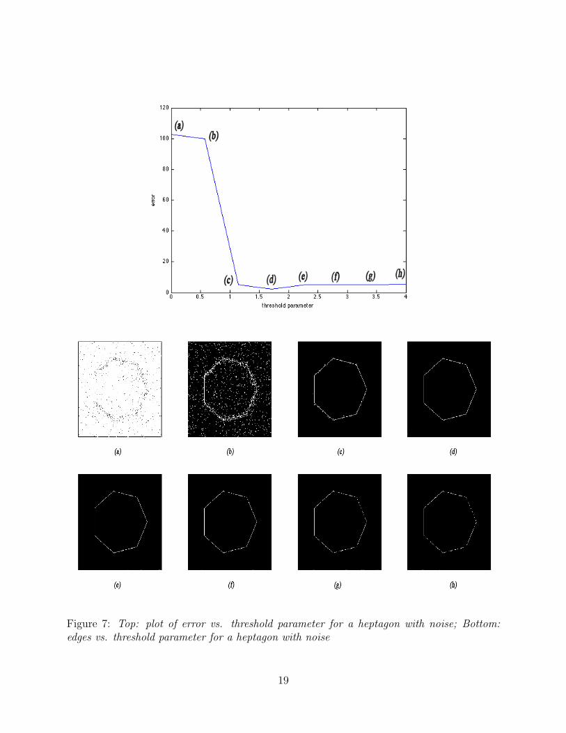
Figure 7: Top: plot of error vs. threshold parameter for a heptagon with noise; Bottom:edges vs. threshold parameter for a heptagon with noise

19

Figure 8: Column 1: a square, a heptagon, an irregular polygon, and cameraman; Column2: the edges, as determined by the Canny method; Column 3: the edges, as determined bythe shearlet method.

20

Figure 9: Top: plot of error vs. threshold parameter for Canny method applied to an irregularpolygon; Bottom: plot of error vs. threshold parameter for shearlet algorithm applied to anirregular polygon; Note that the error continues at a constant value for threshold values upto 1

21