Embed Size (px)
Citation preview
Education Quality and Development Accounting∗
Todd Schoellman†
June, 2011
Abstract
This paper measures the role of quality-adjusted years of schooling in accounting
for cross-country output per worker differences. While data on years of schooling are
readily available, data on education quality are not. I use the returns to schooling of
foreign-educated immigrants in the United States to measure the education quality
of their birth country. Immigrants from developed countries earn higher returns than
do immigrants from developing countries. I show how to incorporate this measure
of education quality into an otherwise standard development accounting exercise.
The main result is that cross-country differences in education quality are roughly as
important as cross-country differences in years of schooling in accounting for output
per worker differences, raising the total contribution of education from 10% to 20%
of output per worker differences.
∗Thanks to Bob Hall, Mark Bils, Pete Klenow, Lutz Hendricks, Scott Baier, Robert Tamura, BertholdHerrendorf, Roozbeh Hosseini, Richard Rogerson, and participants at several workshops, seminars, andconferences for helpful comments and discussion. A particular thanks to Michele Tertilt and ManuelAmador for their gracious guidance throughout this project. The editor and three anonymous refereesprovided many helpful suggestions that substantially improved the paper. Statistics Canada providedcensus data used for the international results. The usual disclaimer applies.†Address: Department of Economics, Arizona State University, Tempe, AZ 85287. E-mail:
1
1 Introduction
Cross-country differences in PPP-adjusted output per worker are large: workers in the
90th percentile of countries are more than 20 times as productive as workers in the 10th
percentile. The development accounting literature attempts to decompose these large cross-
country differences in output per worker into underlying cross-country differences in capital,
human capital, and a residual term typically associated with technology and institutions.1
The goal is to provide quantitative guidance on the proximate sources of output per worker
differences: can they be accounted for primarily by a lack of inputs or by inefficient usage
of inputs?
The current literature focuses on years of schooling as a measure of human capital.
The literature typically finds that years of schooling account for less than 10% of the cross-
country differences in output per worker. The contribution of this paper to the development
accounting literature is to measure the importance of quality-adjusted years of schooling
in accounting for cross-country differences in output per worker. Doing so requires solving
two challenges. The first challenge is to measure education quality differences across coun-
tries. The second challenge is to incorporate measured education quality into development
accounting exercises. I make progress in four steps.
The first step of the paper is to estimate the returns to schooling of foreign-educated
immigrants in the United States.2 I estimate returns for 130 countries, including many
developing countries; there are nine countries in my sample with PPP-adjusted output
per worker less than $1,000. The estimated returns vary by an order of magnitude between
developed and developing countries. For example, an additional year of Mexican or Nepalese
education raises the wages of Mexican or Nepalese immigrants by less than 2 percent, while
an additional year of Swedish or Japanese education raises the wages of Swedish or Japanese
immigrants by more than 10 percent.
The second step of the paper is to provide evidence that these differences in returns
to schooling are due to differences in education quality, and not alternative interpretations
such as selection or skill transferability.3 I show that the estimated returns to schooling are
quantitatively similar for immigrants who enter the United States as refugees and asylees
1See Caselli (2005) for an overview of the accounting literature.2Card and Krueger (1992) first studied returns to schooling of cross-state migrants in the U.S., while
Bratsberg and Terrell (2002) used returns to schooling for immigrants. Both papers focus on estimatingthe education quality production function; this is the first paper to integrate this data into a developmentaccounting exercise.
3The issue of selection was previously raised with respect to Card and Krueger’s work by Heckman,Layne-Farrar, and Todd (1996).
2
and are presumably less selected. I also show that the returns to schooling are corre-
lated with another measure of education quality, the scores on internationally standardized
achievement tests. In my empirical implementation, I exploit this correlation to use test
scores as an instrument for the returns to schooling, adding a further correction for the
selection of immigrants.4
The first two steps provide a measure of education quality, namely the returns to school-
ing of foreign-educated immigrants. The third step of the paper is to measure the role of
education quality in producing human capital. I follow in the footsteps of Bils and Klenow
(2000) by specifying a human capital production function, now augmented to allow for
education quality differences. I use the predictions of a simple school choice model in the
spirit of Mincer (1958) and Becker (1964) to estimate the key parameter of the human
capital production function, which governs the elasticity of school attainment with respect
to education quality.
The fourth step of the paper is to combine the human capital production function and
measured education quality to construct estimates of human capital stocks around the
world. The baseline finding of this paper is that education quality differences are roughly
as important as years of schooling differences. Alternatively, I find that incorporating
education quality differences doubles the role of human capital in accounting for cross-
country output per worker differences. To put this number into an absolute perspective,
Hall and Jones (1999) find that replacing the poorest country’s years of schooling with U.S.
years of schooling would raise their output per worker from 3% to 7.5% of the U.S. level.5
This paper’s methodology implies that replacing their years of schooling and education
quality with U.S. years of schooling and education quality would raise their output per
worker from 3% to 20% of the U.S. level. I argue that this finding is robust to several
possible extensions of the accounting framework.
The most closely related paper in the literature is by Hendricks (2002), who also uses
the wages of U.S. immigrants to estimate cross-country differences in human capital stocks.
4Some previous research has used test scores as a measure of education quality (Caselli 2005, Hanushekand Kimko 2000, Hanushek and Woessmann 2009). I do not use test scores as a direct measure of educationquality because their scale is difficult to use in a development accounting exercise. Test scores show that theaverage student in one country scores one standard deviation higher than the average student in anothercountry, but it is difficult to translate this difference into the relative value of a year of each country’sschooling. Returns to schooling show that the wage gain of a year of one country’s schooling is twice thewage gain of another country’s schooling; under certain conditions explored in the model, this statementimplies that each year of the former country’s schooling generates twice as much human capital.
5Most of the literature values years of schooling differences using the pioneering work of Bils and Klenow(2000). Bils and Klenow also consider a separate methodology to account for education quality, discussedbelow. Since Hall and Jones it has been common in the literature to ignore education quality.
3
His approach uses the average wage difference between natives and immigrants, which he
finds to be small. If immigrants are unselected, this finding implies that human capital
differs little between natives and non-migrants. However, recent papers in the literature
have noted that Hendricks’ results are also consistent with modest positive selection of
immigrants and modestly larger differences in human capital between natives and non-
migrants (Manuelli and Seshadri 2007). The approach in this paper uses the average wage
difference between immigrants from the same country with different levels of education as
the main wage statistic. This statistic is a narrower measure of education quality, and is
less likely to be affected by the selection of immigrants.
My paper is also related to a previous literature on cross-country differences in edu-
cation quality. Since data on education quality is scarce, most research has been driven
by models of the education quality production function. Typically student time is aug-
mented by teacher quality or expenditures as in Ben-Porath (1967).6 This paper provides
new estimates of education quality and its importance that are independent of any educa-
tion quality production function. Independence is a virtue since the education literature
is unclear about what attributes produce education quality, and provides a wide range of
estimates for education quality production functions; see Hanushek (1995) and Hanushek
(2002) for an overview. In particular, while expenditure on education is often thought to
be an important way to improve quality, there is little empirical guidance on the size of
the channel. Hence, outside evidence can provide a useful check for this literature. On
the other hand, the primary deficiency of not specifying a production function is that this
paper cannot provide policy prescriptions since it is agnostic about the sources of what are
measured to be large quality differences. Their work provides insight on this subject.
The paper proceeds as follows. Section 2 estimates the returns to schooling of immi-
grants and shows that they cannot be explained easily through selection or skill transfer-
ability. Section 3 gives the baseline development accounting results. Section 4 considers
extensions to the model and shows that the accounting results are robust. Section 5 con-
cludes.
6See Bils and Klenow (2000) for teacher quality, Manuelli and Seshadri (2007), Erosa, Koreshkova, andRestuccia (2010), Cordoba and Ripoll (2010), and You (2008) for expenditures, and Tamura (2001) forboth.
4

2 Returns to Schooling of Immigrants
The first step of the paper is to estimate the returns to schooling of foreign-educated
immigrants to the United States. The estimation follows in the path of Card and Krueger
(1992), who use the returns to schooling of cross-state migrants within the United States
to infer the education quality of states. The idea was previously extended to cross-country
immigrants by Bratsberg and Terrell (2002); I update their exercise using 2000 U.S. census
data. The U.S. census is ideal because it contains a large sample of immigrants from many
different countries, includes a large set of controls such as English language ability, and
provides the variables necessary to impute which immigrants completed their schooling
abroad.
Following Card and Krueger (1992), I estimate the returns to schooling of immigrants
using an augmented Mincer wage equation:
log(W j,kUS) = γjUS + µjUSS
j,kUS + βXj,k
US + εj,kUS. (1)
I adopt the convention that superscripts distinguish workers k and their country of birth
j, while subscripts denote the country of observation, typically the United States. The
regression equation says that the log of wages W are determined by an intercept term;
years of schooling S; a vector of common controls X that includes for example potential
experience; and an error term ε. A standard Mincerian wage equation might use only
Americans, and would have a single intercept γ and a common return to schooling µ. The
above wage equation is augmented in allowing both the intercept of log-wages and the
return to schooling to vary based on the immigrant’s country of birth.
In this paper, I focus on the country-specific return to schooling µjUS and ignore the level
differences γjUS.7 In a cross-section of Mexican or Vietnamese immigrants in the United
States, an additional year of schooling is associated with small wage gains; in a cross-
section of Swedish workers, an additional year of schooling is associated with large wage
gains. I discard the level of the wage profile because it may be influenced by selection of
immigrants or other factors unrelated to education quality. I return to this idea below. As
is common in studies using immigrants not all parameters of equation (1) are well-identified,
but Appendix A shows that the country-specific return to schooling is.
I implement this equation using the 5% sample of the 2000 census Public Use Micro
7Hanushek and Kimko (2000) previously showed that immigrants from countries with high test scoresearn higher average wages in the United States; my findings are consistent with theirs but differ in usingthe return to schooling rather than the average wage.
5

Survey, made available through the IPUMS system (Ruggles, Alexander, Genadek, Goeken,
Schroeder, and Sobek 2010). Immigrants are identified by country of birth.8 The census
lists separately each of 130 statistical entities with at least 10,000 immigrants counted in
the United States. Some of these statistical entities are nonstandard: for instance, there are
response categories for Czechoslovakia, the Czech Republic, and Slovakia, since immigrants
came both before and after the split. I refer to these statistical entities as countries as a
shorthand. I keep as many countries as are separately identified, except that the United
Kingdom is merged into a single observation.
The census includes a measure of schooling attainment which I recode as years of school-
ing in the usual manner. The census does not provide direct information on where the
schooling was obtained. Instead I use information on age, year of immigration, and school-
ing attainment to impute which immigrants likely completed their schooling abroad. It is
important to exclude from the sample immigrants who may have received some or all of
their education within the United States to have an unbiased estimate of source-country ed-
ucation quality. My baseline sample includes immigrants who arrived in the United States
at least six years after their expected date of graduation to minimize measurement error
from immigrants who repeat grades, start school late, or experience interruptions in their
education. Thus, high school graduates have to be at least age 24 when they immigrate
to be included (expected to complete at age 18, plus six years as a buffer). I also select
workers who are strongly attached to the labor market, meaning those aged 18-65 who
were employed for wages (not self-employed), who reported working at least 30 weeks in
the previous year and at least 30 hours per week, and who have between 0 and 40 years of
potential experience. The first benefit of working with the 2000 U.S. census is that it is a
large sample with many immigrants. Even after imposing these sample selection criteria I
have a final sample with 4.1 million Americans and 210,000 immigrants.
I calculate the wage as the previous year’s average hourly wage, computed using annual
wage income, weeks worked, and usual hours per week. The census includes a rich set
of control variables. I include several standard controls such as a quartic in potential
experience and a full set of dummy variables for census region of residence, gender, disability
status, and living in a metropolitan area. The census also offers two control variables
that are particularly useful in the case of immigrants. It asked respondents to self-report
English language proficiency on a five option scale; it also collected information on year
of immigration. I enter each as a full set of dummy variables. These last two terms help
8A potential bias could arise if immigrants are born in one country but receive their schooling in another.However, 89% of immigrants who were living abroad five years prior to the census were living in their birthcountry.
6
capture the fact that immigrants’ labor market prospects may be limited by language or
may be limited upon initial arrival to the United States.
2.1 Estimates and Baseline Interpretation
Appendix B provides the key estimates of this regression, µjUS, as well as the standard error
of the estimates and the number of observations per country. The results are ordered by
rate of return so that the large differences are immediately apparent. The measured U.S.
return provides a benchmark of 11.1% per year. Immigrants from several countries earn
higher rates of return, including two with statistically significant returns over 12% per year,
Japan and Switzerland. At the other end of the spectrum some countries have remarkably
low returns, including one with negative but imprecisely estimated returns to schooling.
Two useful benchmarks on the low end are Mexico and Vietnam. Since each country has a
large number of immigrants in the United States, they have reasonably precisely estimated
returns of 1.8% and 2.8% per year of schooling.
TONALBMKD
LAONPL CPVKHM MEXHND BIHSLV GTMSOM SLE PRTSDN DOMBOLVNM ECUERI CUBARM IRQNIC
LBR BLZJORPER CRI KORUZB THACOLYEMHTIUGA POLSENBGDETH SYR WSMMDA CYPNGA HRVPRY LVAGHA ESPDMA SAUAZE GRDTTO PRICZE FINEGYPAK BRABGRCMRIDNGUY DZA AUTVENPHL BHSROM TUR ITABLRJAM LCAUKRGEO PAN GRCCHN CHLFJILKA LTU IRNIND BRBARGKEN IRLTWNFRAMYSVCTMAR LBN HKGISRURYSVK DNKSGPZWE NZL AUSCANGERBELGBRZAF USANLDNORHUN KWTSWEJPN
CHETZA
0.0
5.1
.15
Est
imat
ed R
etur
n to
Sch
oolin
g of
Imm
igra
nts
7 8 9 10 11 12Log PPP GDP p.w.
Baseline Estimates Regression Line
(a) Output per Worker
ALBMKD
MEXPRTSRB
ARMJORPER KORTHACOL POL
MDACYPNGA LVAGHA ESPSAU CZEFINEGYBRA BGRIDN AUTPHL ROMTUR ITAGRC CHNCHL LTUIRNINDARG IRL TWNFRAMYSMAR LBN HKGISRURY SVKDNK SGPZWE NZLAUSCANGERBELGBRZAF USA NLDNOR HUNKWT SWE
JPNCHE
0.0
5.1
.15
Est
imat
ed R
etur
n to
Sch
oolin
g of
Imm
igra
nts
3 3.5 4 4.5 5 5.5International Test Scores
Baseline Estimates Regression Line
(b) Test Scores
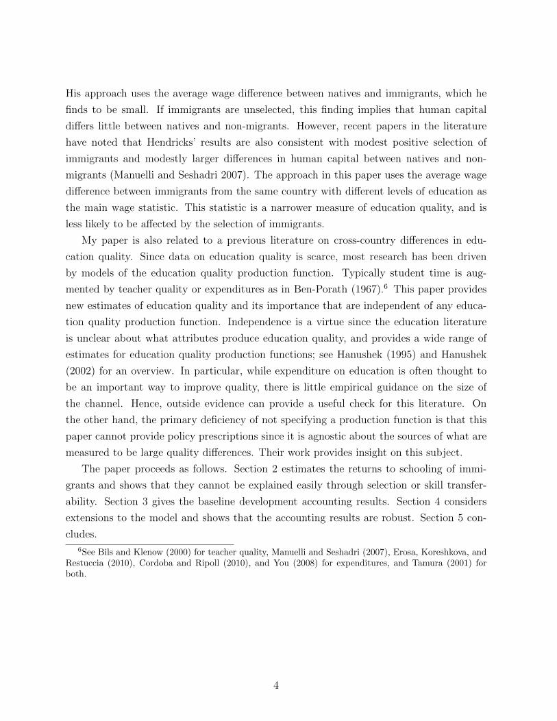
Figure 1: Patterns for Returns to Schooling of Immigrants
Figure 1a plots the estimated returns to schooling of immigrants against the log of PPP
GDP per worker from the Penn World Tables (Heston, Summers, and Aten 2009). It shows
already the first punchline of the paper: immigrants from developed countries earn higher
returns on their foreign schooling than do immigrants from developing countries. Some
of the estimated returns to schooling plotted on the y-axis are based on small samples
of immigrants and are somewhat imprecise; for example, the obvious outlier of Tanzania
is based on just 73 immigrants. For this and most subsequent figures, I also include the
7

fitted line from a weighted regression using number of immigrants in the sample as the
weights. This regression and all subsequent weighted regressions exclude the U.S. and
Mexico. Mexican immigrants are roughly one-third of the total immigrant sample, and
there is a concern that their experience may be atypical.
The baseline interpretation of the relationship in figure 1a is that it is the result of
differences in education quality between developed and developing countries. Figure 1b
offers some evidence for this point of view. It plots again the estimated returns to schooling
of immigrants, this time against test scores from internationally standardized achievement
tests. These scores come from testing programs that administer comparable exams to
randomized samples of students still enrolled in school at a particular age or grade in a
variety of countries.9 The data used here were constructed by Hanushek and Woessmann
(2009) by aggregating the results from a number of tests administered between 1964 and
2003. The figure shows that on average, immigrants from higher test score countries earn
higher returns on their schooling in the United States. The intuition is that high-quality
education imparts more human capital per year of schooling, which in turn is associated
with a larger wage gain per year of schooling.
If the returns to schooling of immigrants measure the education quality of their birth
country, then figure 1a has an important message. In addition to the well-known fact that
workers in developed countries have higher schooling attainment, each of those years of
schooling is also of higher quality. Section 3 shows how to incorporate an education quality
adjustment into development accounting exercises. First, I discuss the robustness of the
findings in figure 1 and provide evidence against plausible alternative interpretations.
2.2 Robustness
The estimated returns to schooling of immigrants are robust to many of the details of sample
selection and to the control variables used. For example, excluding immigrants who entered
the United States less than three or nine years after their expected date of graduation
(instead of six years in the baseline) does not affect the results. Neither does allowing
for interactions between potential experience and country of birth. I also experiment with
allowing returns to schooling to vary by English-language ability or years since immigration
and find little difference in estimated returns to schooling. A supplementary appendix
9In practice countries vary in their exclusion and non-response rates so that samples are not perfectlyrandom. Hanushek and Woessmann (2011) document that variation in the sample can account for some ofthe differences in average test scores by country. They find that even after controlling for this effect, testscores still predict growth rates.
8

available online provides details of how robustness checks were performed as well as the
results.
If the returns to schooling of immigrants measure their education quality, then returns
should be quantitatively similar in other data sets. I focus on two data sets that provide a
large number of immigrants from many countries: the 1990 U.S. census, and the 2001 Cana-
dian census.10 The Canadian census is particularly interesting since it gives results from
a different country with different immigration rules and labor market institutions, which
could affect the measured returns to schooling. For example, Antecol, Cobb-Clark, and
Trejo (2003) document that while around two-thirds of American immigrants enter based
on family relationships with current citizens or residents, only one-third of Canadian immi-
grants do so. Conversely, while less than 10% of American immigrants enter based on labor
market skills, around one-third of Canadian immigrants enter through a ‘points’ system
that rewards education, English fluency, and other skills. If returns to schooling measure
education quality, then they should be consistent across these two different immigration
policies.
PRT
VNM
YUG
POL
PHLITA
GRC
CHN
IND FRA
HKG
CAN
GER
GBR
USA
0.5
11.
52
Nor
mal
ized
Ret
urn
to S
choo
ling
of Im
mig
rant
s
0 .5 1 1.5Normalized Return to Schooling of Immigrants (2000 U.S.)
Estimates Regression Line
(a) 2001 Canadian census
AZO
LAOCPV
KHMMEX
HND
SLVGTM
PRT
DOMBOLVNMECU
CUBIRQ
NIC
BLZ
PER
CRI
KOR
YUGTHACOL
HTIPOL
BGD
ETH
SYR
NGA
GHA
ESP
DMA
GRD
MMR
TTOPRI
EGYPAK
BRA
IDN
GUYAUT
CSK
VEN
PHLROM
TUR
ITA
JAM
AFG
PAN
GRC
CHN
CHL
FJI
LKA
IRN
INDBRBARG
IRL
TWN
FRA
MYS
LBN
HKG
ISR
URYAUS
CANGERGBR
ZAF
USA
NLD
HUN
SWE
JPN
CHE
0.2
.4.6
.81
Nor
mal
ized
Ret
urn
to S
choo
ling
of Im
mig
rant
s
0 .5 1 1.5Normalized Return to Schooling of Immigrants (2000 U.S.)
Estimates Regression Line
(b) 1990 U.S. census
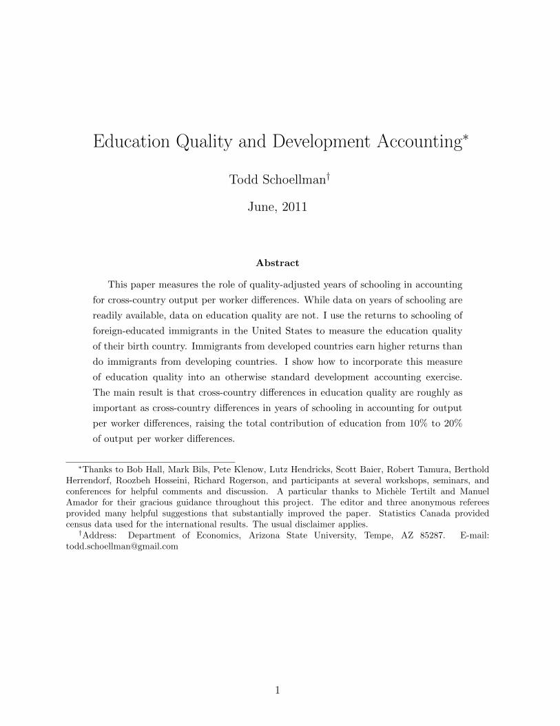
Figure 2: Returns to Schooling of Immigrants Estimated from Other Samples
These censuses provide very similar information as compared to the 2000 U.S. census,
so that estimation of the returns to schooling is quite comparable in terms of sample selec-
tion, variable construction, and controls included. Figure 2 plots the estimated returns to
schooling of immigrants from the 2001 Canadian census and the 1990 U.S. census against
10The 1990 U.S. census is also available from Ruggles, Alexander, Genadek, Goeken, Schroeder, andSobek (2010); the Canadian census is available through Minnesota Population Center (2010).
9

the baseline estimates from the 2000 U.S. census. In all three samples I have normalized the
estimated returns by the returns to schooling for Americans (natives in the U.S. samples,
immigrants in the Canadian sample) to eliminate variation in the skill premium. Figure
2a shows that the returns to schooling are very similar between the United States and
Canada despite differences in immigration policy. Figure 2b shows that the returns within
the United States are consistent back to 1990.
Given the results of figure 2 I conclude that the estimated returns to schooling are
quantitatively robust. The next question is whether there are plausible alternative inter-
pretations, based on selection or skill transferability. The returns to schooling of immigrants
from developed countries are typically 8-12%, not very different from the return to school-
ing for Americans of 11.1%. Hence, I focus on the question of whether the low observed
returns to schooling for immigrants from developing countries, such as the 1.8% return to
schooling for Mexican immigrants, can be explained by selection or skill transferability.
2.3 Selection Interpretation
A potential concern with estimating the returns to schooling of immigrants is that they may
be affected by selection. Immigrants are potentially selected in two ways: first, they are self-
selected, since they have typically decided to come to the United States; and second, they
are selected by U.S. immigration policy if they enter the country through formal channels.
This section explores what types of selection would explain the relationship between returns
to schooling of immigrants and output per worker, and provides some evidence concerning
selection.
To motivate the selection discussion it is helpful to repeat the augmented Mincer wage
equation:
log(W j,kUS) = γjUS + µjUSS
j,kUS + βXj,k
US + εj,kUS.
If immigrants are selected on observable characteristics, such as potential experience or
schooling, this is directly controlled for in the wage equation. The more important con-
cern is that they may be selected on unobservable characteristics. Some of the effects of
selection are captured by country of origin fixed effects γj, which I discard. For example,
suppose that Mexican immigrants with different school attainments are all equally selected:
they have unobserved ability that causes them to earn 10% more in labor markets than a
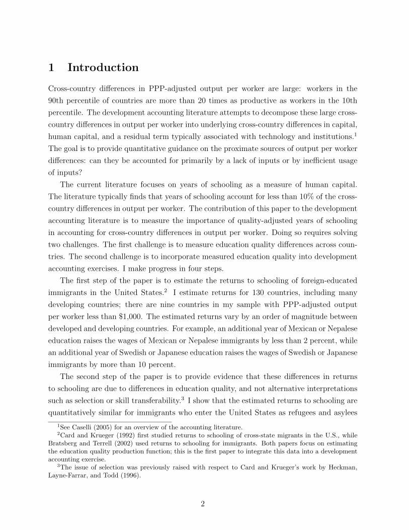
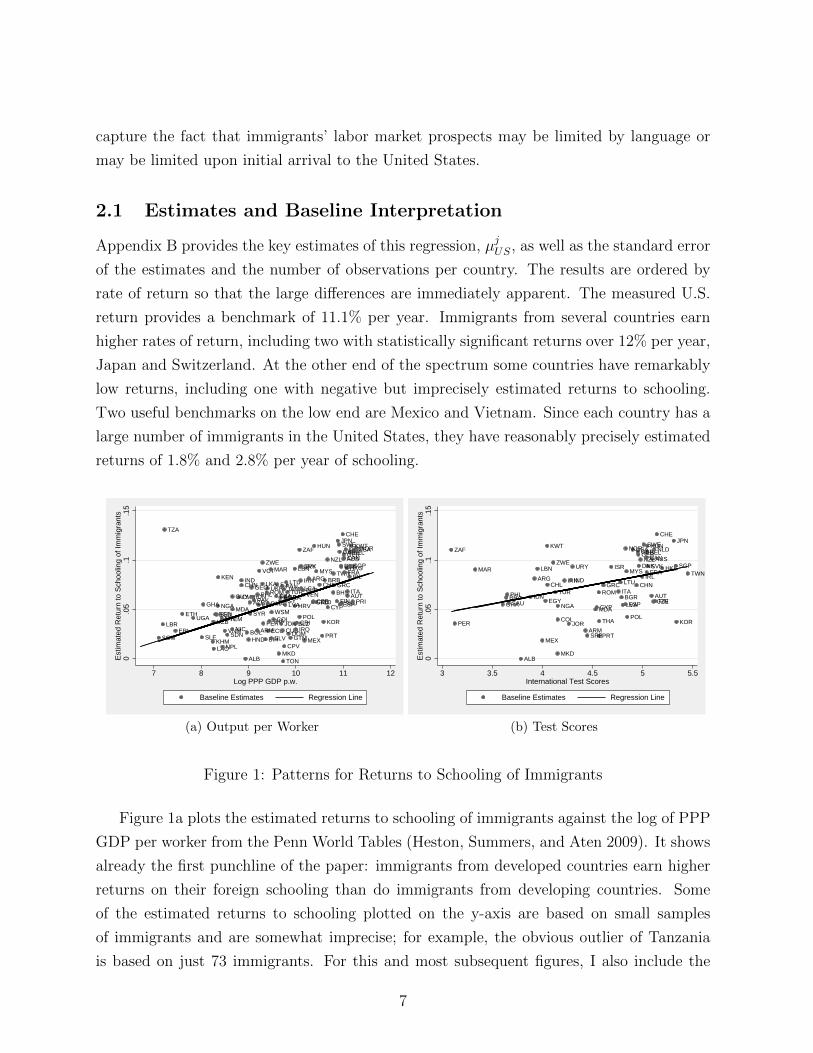
randomly chosen Mexican worker with the same school attainment. Figure 3a shows what
this selection implies for the relationship between log-wages and schooling. The solid line
10

is the observed wages of Mexicans who immigrated: the returns to schooling are a modest
1.8% per year. If Mexicans immigrants with different school attainments are all equally
selected, then the dashed line is the implied wages that would be observed for an random
sample of Mexicans. This selection affects the intercept γMexico, which explains why I do
not use the intercepts. However, it does not affect the measured returns to schooling.
By discarding the fixed effects, this paper is robust to some of the immigrant selection
concerns that apply to Hendricks (2002). Hendricks uses a non-parametric estimate of
immigrant wages that is close in spirit to regressing
log(W j,kUS) = γj + µSj,kUS + βXj,k
US + εj,kUS (2)
although he does not impose linearity restrictions. This regression differs from mine only in
the fact that it restricts the return to schooling µ to be the same for all countries, whereas
I allow for differences in µjUS.
Hendricks measures unobserved human capital (human capital not related to years of
schooling or potential experience) using the level difference in wages, similar to γj−γUS. The
differences in wages between natives and immigrants with similar observed characteristics
are small, implying that natives and immigrants differ little in their unobserved human
capital. Hendricks draws two inferences. First, if immigrants are unselected, then the small
wage differences between natives and immigrants implies small unobserved human capital
differences around the world, and a small role for unobserved human capital in accounting
for cross-country output per worker differences. Second, he uses a bounding argument to
show that immigrants would have be selected to an implausible degree for human capital to
account for all of the cross-country differences in output per worker. However, recent papers
have noted that his wage results are also consistent with a modest degree of selection and
a modestly larger role for human capital than his baseline results might suggest (Manuelli
and Seshadri 2007). This insight is motivated in part by the fact that Hendricks’ estimates
suggest immigrants from 28 of the 66 countries in his sample have more unmeasured human
capital than do Americans, including immigrants from Turkey, Syria, and Hungary.
I use the returns to schooling of immigrants rather than average wage differences to help
reduce selection problems and narrow the range of plausible estimates for cross-country dif-
ferences in human capital per worker. However, returns to schooling can also be affected
by selection of two forms. First, if there is within-country heterogeneity in the return to
schooling, then immigrants could be selected based on this return. In section 4.2 I incor-
porate heterogeneity in the return to schooling into my model and show that the model’s
11
S
log(W)
μRandom Sample =1.8%
μImmigrants = 1.8%Selection
γImmigrants
γNo Selection
(a) Selection
S
log(W)
μRandom Sample =11.1%
μImmigrants = 1.8%
Selection
(b) Differential Selection
Figure 3: Effect of Two Types of Selection on Estimation Results
predictions are at odds with the hypothesis that low returns to schooling in developing
countries are due to selection on the return to schooling. Since this discussion requires the
model, I delay it for now. A second possibility is that immigrants with different education
levels are differentially selected on γjUS, indicating that in fact the intercept is γjUS(S).11
Specifically, suppose that the returns to schooling for a randomly selected group of Mexican
workers would have been 11.1%, the same as Americans. The observed return to schooling
for immigrants is 1.8%. Figure 3b shows how these two statements could be consistent: it
must be that immigrants with lower education levels are more selected. Further, recall that
the returns to schooling for immigrants from developed countries are about the same as
the returns to schooling for Americans. For selection to explain my results, it must be that
less educated immigrants from developing countries are differentially selected, but that less
educated immigrants from developed countries are not.
It may be plausible that some form of policy selection or self-selection of immigrants
could generate this pattern of differential selection. To investigate whether this is the case,
I turn to evidence drawn from a relatively less selected group of immigrants: refugees and
asylees. Refugees and asylees are less likely to be affected by both forms of selection.
They are fleeing persecution, war, or other violence, and so are less prone to self-selection.
Further, U.S. immigration policy includes a commitment to resettle at least 50 percent of all
refugees referred for consideration by the United Nations High Commissioner for Refugees,
on explicitly humanitarian grounds.12 Hence, refugees and asylees are less selected by
11I am indebted to an anonymous referee for this hypothesis.12United States Department of State and United States Department of Homeland Security and United
States Department of Health and Human Services (2009).
12

immigration policy, as well. Previous work has shown labor market differences between
refugees and non-refugees, including a large earnings gap between refugees and non-refugees
(Cortes 2004, Jasso, Massey, Rosenzweig, and Smith 2000). Hence, I ask whether the
returns to schooling of refugees and asylees look different from the returns to schooling of
other migrants, who are collectively called economic migrants.
The census does not identify whether immigrants were refugees/asylees, but it does
identify the country of their birth and the year of their immigration. The Statistical Year-
book of the Immigration and Naturalization Service from 1980-2000 identifies the fraction
of each country’s immigrants for that year that were refugees/asylees and the fraction that
were economic migrants. I identify 18 countries whose immigrants to the United States were
at least 50% refugees/asylees for at least five consecutive years. I estimate the returns to
schooling for immigrants in the census who were born in these countries and immigrated in
these years. I also identify 82 countries whose immigrants to the United States were never
more than 10% refugees/asylees for any year from 1980-2000, and estimate the returns to
schooling for immigrants in the census who were born in these countries and immigrated
in these years.
SOM
ETH
KHMUZBLAO
VNMSDN
MDA
AZE
BIH
ROMUKR
THAIRQ
BLR
HUN
0.0
5.1
.15
Est
imat
ed R
etur
n to
Sch
oolin
g of
Imm
igra
nts
7 8 9 10 11 12Log PPP GDP p.w.
Estimates Regression Line
(a) Refugees/Asylees
TZA
ERI
SLE
GHA
BGDSEN
NGAYEM
GUYCMR
INDCHN
BOLHND
PAK
ARM
PHL
PRY
VCT
LKA
ZWE
PER
DMA
ECU
MAR
SLV
WSM
COL
DZA
FJI
EGY
JOR
PAN
TON
JAM
CPV
BRA
DOMGTM
LBN
BLZCRI
ZAF
URY
LCAVEN
MEX
ARG
GRDTTO
CHL
PRT
KOR
BRB
NZL
CYP
TWN
GRC
FIN
JPNSWEGBR
ESP
DNKISR
CHE
AUSGERCAN
FRA
NLD
HKGITA
IRL
BEL
SGP
KWTNOR
0.0
5.1
.15
Est
imat
ed R
etur
n to
Sch
oolin
g of
Imm
igra
nts
7 8 9 10 11 12Log PPP GDP p.w.
Estimates Regression Line
(b) Economic Migrants
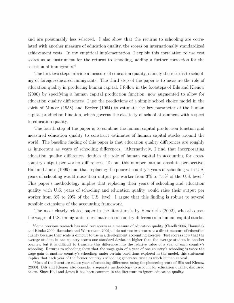
Figure 4: Returns to Schooling for Refugees/Asylees and Economic Migrants
Figure 4 plots the returns to schooling for refugees/asylees and economic migrants
against the log output per worker of the country. A quantitatively similar relationship
prevails for both groups, although the slope of the trend line for refugees is significant at
the 10% rather than 5% level. Further, refugees from a number of developing countries
earn low returns to schooling, including Cambodia, Somalia, Sudan, and Laos.
13
The low estimated returns to schooling for refugees from these countries are unlikely
to be explained by a selection story. To see why, consider the case of Cambodia. Around
600,000–800,000 Cambodians were killed as the country slipped into chaos in the early
1970s, and then another 1 million under the Khmer Rouge regime that ruled from 1975 to
1978. As the Khmer Rouge began to lose control of the country, several hundred thousand
Cambodians fled to Thailand and were placed in refugee camps. Around 150,000 of these
refugees were resettled in the United States; between 1980 and 1991, 99.5% of immigrants
from Cambodia were refugees. The refugees represented a broad swathe of society consisting
mostly of those who were able to flee (Mortland 1996). Yet the estimated return to schooling
for Cambodians entering the United States in these years is just 1.6% per year of schooling.
2.4 Skill Transferability Interpretation
Immigrants from developing countries earn low returns to their education, even if they
enter the countries as refugees and asylees, who are less selected than the typical immigrant.
However, a second potential concern with estimating the returns to schooling of immigrants
is that they may reflect the difficulty immigrants face in translating their foreign skills to
the U.S. labor market, rather than a lack of skills. This difficulty could arise if immigrants
find it difficult to apply their skills, or if U.S. labor markets erect barriers that prevent
immigrants from exercising their skills.
I present three pieces of evidence against this hypothesis. First, the estimated returns
to schooling are similar in Canada, although Canadian immigration policy is more skill-
oriented than is U.S. immigration policy. Second, there are large differences in the estimated
returns to schooling even among immigrants who have been in the United States for fif-
teen years and speak English very well. I have estimated returns to schooling separately
for immigrants who entered the United States before and after 1985, and separately for
immigrants with and without strong English skills. For each case the estimated returns are
quantitatively similar to the baseline estimates. Hence, differences in returns to schooling
persist even for immigrants who have had time to assimilate and who have the language
skills to bring their education to bear.
Finally, I explore whether restrictions in the U.S. labor market prevent immigrants from
using their skills. In particular, I estimate separately the return to schooling for immigrants
who work in licensed and unlicensed occupations. Licensure is the strongest form of occupa-
tional restriction: workers are required to obtain a license from the government to practice
their profession. To the extent that low returns to schooling are explained by restrictions
that prevent immigrants from exercising otherwise valuable skills, then workers who are
14

able to secure a license should presumably earn a rate of return commensurate with their
education quality, while workers in unlicensed occupations should presumably earn a lower
rate of return. I use licensure data from CareerOneStop (2010), which is sponsored by the
U.S. Department of Labor. I define an occupation as licensed if it is federally licensed, or
if it is in the top decile in terms of licenses issued at the state level; all other occupations
are classified as unlicensed. The list of licensed occupations is heavily weighted towards fi-
nancial services, engineering, and medical and teaching professionals. It also includes some
less-skilled occupations such as hairdresser, which is licensed in many states.
LAO MEXHNDBIHSLV
GTMSLE
PRT
DOM
VNM
ECU
CUB
IRQ NIC
LBR
PER
CRI
KOR
YUG
THA
COLHTI
POLBGD
ETH
NGA
GHAESP
GRD
TTO PRI
EGY
PAKBRABGR
IDN
GUY
VEN
PHLROM
TURITA
BLR
JAM
AFG
UKR
PANGRC
CHNCHL
LKA
IRN
IND
BRB
ARG
KEN
IRLTWN
FRA
MYS
LBN
HKG
ISRNZL
AUS
CAN
GER
GBR
ZAF
USANLD
JPN
0.0
5.1
.15
Ret
urns
to S
choo
ling
of Im
mig
rant
s (L
icen
sed)
0 .05 .1 .15Returns to Schooling of Immigrants (Unlicensed)
Estimates Regression Line
Figure 5: Returns to Schooling of Immigrants in Licensed and Unlicensed Occupations
Figure 5 plots the estimated returns to schooling for immigrants in licensed occupations
against the estimated returns to schooling for immigrants in unlicensed occupations. The
figure is restricted to countries with at least 50 workers in each category, and shows quan-
titatively similar returns for the two groups. The trend line from a weighted regression is
also included; it is positive and significant. Formal licensure does not explain why returns
to schooling for immigrants from developing countries are so low. Since the evidence also
points against a selection interpretation, I use the returns to schooling of immigrants as a
measure of education quality for the remainder of the paper. I now turn to incorporating
these estimates into development accounting exercises.
3 Baseline Accounting Model
The previous section documented large and persistent differences in the returns to schooling
of immigrants from developed and developing countries. The baseline interpretation of these
returns is that they are measures of the education quality of different countries. This section
15
incorporates these measures of education quality into an otherwise standard development
accounting exercise.
The production side of the economy is similar to the development accounting literature
such as Hall and Jones (1999) or Caselli (2005). A country’s output per worker is related
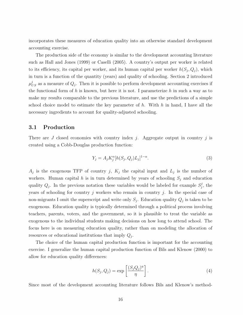
to its efficiency, its capital per worker, and its human capital per worker h(Sj, Qj), which
in turn is a function of the quantity (years) and quality of schooling. Section 2 introduced
µjUS as a measure of Qj. Then it is possible to perform development accounting exercises if
the functional form of h is known, but here it is not. I parameterize h in such a way as to
make my results comparable to the previous literature, and use the predictions of a simple
school choice model to estimate the key parameter of h. With h in hand, I have all the
necessary ingredients to account for quality-adjusted schooling.
3.1 Production
There are J closed economies with country index j. Aggregate output in country j is
created using a Cobb-Douglas production function:
Yj = AjKαj [h(Sj, Qj)Lj]
1−α. (3)
Aj is the exogenous TFP of country j, Kj the capital input and Lj is the number of
workers. Human capital h is in turn determined by years of schooling Sj and education
quality Qj. In the previous notation these variables would be labeled for example Sjj , the
years of schooling for country j workers who remain in country j. In the special case of
non-migrants I omit the superscript and write only Sj. Education quality Qj is taken to be
exogenous. Education quality is typically determined through a political process involving
teachers, parents, voters, and the government, so it is plausible to treat the variable as
exogenous to the individual students making decisions on how long to attend school. The
focus here is on measuring education quality, rather than on modeling the allocation of
resources or educational institutions that imply Qj.
The choice of the human capital production function is important for the accounting
exercise. I generalize the human capital production function of Bils and Klenow (2000) to
allow for education quality differences:
h(Sj, Qj) = exp
[(SjQj)
η
η
]. (4)
Since most of the development accounting literature follows Bils and Klenow’s method-
16

ology to account for years of schooling, this functional form will make my results for
quality-adjusted years of schooling directly comparable to the literature. By interacting
education quality in the exponent, I produce the result (explored below) that education
quality and years of schooling are positively correlated as long as 0 < η < 1. I view this
result as desirable since there is significant microeconomic evidence supporting such a pos-
itive correlation (Case and Deaton 1999, Hanushek, Lavy, and Hitomi 2008, Hanushek and
Woessmann 2007).13
Given this functional form, I have almost all the ingredients to construct the human
capital stocks of countries. Sj is known from Barro and Lee (2001), and I have estimated
Qj = µjUS. The last component is an estimate of η. To find such an estimate, I write
down a simple model of school outcomes. A representative firm hires efficiency units of
labor and pays a wage per efficiency unit. Workers make a school choice along the lines of
Becker (1964) and Mincer (1958). This model makes an equilibrium prediction about the
relationship between Sj and Qj that depends on η; I estimate the values of η so that the
model-predicted relationship between Sj and Qj is consistent with the data. Given this
final ingredient, I can conduct development accounting exercises.
3.2 Firm’s Problem
The representative firm takes prices, wages, and rental rates as given. It hires labor and
rents capital to maximize profits. I assume that the price of the final good is the numeraire,
so that the firm’s problem is:
maxKj ,Hj
AjKαj H
1−αj − (rj + δ)Kj − wjHj
where I have omitted time indices since the firm’s problem is static. Hj = hjLj is the total
efficiency units of labor hired by the firm. I use wj to denote the wage rate per unit of
human capital and Wj = wjhj to denote the hourly wage of an individual with hj units of
human capital.
3.3 Worker’s Problem
Each economy has a continuum of measure 1 of ex-ante identical dynasties. A dynasty is a
sequence of workers who are altruistically linked in the sense of Barro (1974). Each worker
13Bils and Klenow (2000) explored adding education quality of the form h(Sj , Qj) = Qj exp(Sηj /η
). This
way of modeling education quality has the drawback that it does not affect equilibrium school attainmentin simple models of school choice, contrary to the data.
17

lives for T years, then dies and is replaced by a young worker who inherits his assets but
not his human capital. Hence, it is the death of members of the dynasty that motivates
further education. The date of death is staggered so that 1/T workers die in each year.14
Workers are endowed with one unit of time each period to allocate between school and
work. They have no direct preferences over school or work, so their school choice is made to
maximize lifetime income net of tuition costs. While in school workers pay tuition λj(S, t)
and forego labor market opportunities, but acquire human capital. Upon entry into the
labor market, workers’ earnings are determined by the wage per unit of efficiency labor
wj(t) and their human capital h(S,Qj). Workers discount future tuition payments and
earnings using a constant interest rate rj. I further assume that the wage rate grows at a
constant rate gj, so that wj(t) = wj(0)egjt, where gj is determined by the growth rate of
Aj on a balanced growth path. I follow Bils and Klenow (2000) in assuming that tuition
is a country-specific multiple of the foregone wage, λj(S, t) = λjwj(t)h(τ + t, Qj). This
assumption captures the fact that tuition payments tend to rise with schooling attainment,
and gives convenient closed form solutions.
Workers take wage rates, interest rates, tuition rates, and education quality as given
and choose schooling to maximize lifetime income net of tuition costs. The standard result
in this model is that workers separate their lives into two periods: they go to school full-
time from the beginning of their life until some endogenously chosen age S; then they work
full-time until they die. The problem of a worker born at τ is then given by:
maxS
∫ τ+T
τ+S
e−rjtwj(0)egjth(S,Qj)dt−∫ τ+S
τ
e−rjtλjwj(0)egjth(τ + t, Qj)dt.
3.4 Equilibrium School Attainment
Combining the solutions to the problem of the representative firm and the workers yields
the equilibrium outcome for schooling:
Sj =
[Qηj
Mj
]1/(1−η)
. (5)
Schooling is increasing in education quality and decreasing in Mj, where Mj denotes the
Mincerian (log-wage) return to schooling for non-migrants, or the return to schooling for a
Swede who stays in Sweden. Mj is the standard Mincerian return to schooling discussed in
14I ignore differences in mortality across countries because incorporating life expectancy as differences inTj was found to be unimportant in earlier versions of the paper.
18

the development accounting literature; Psacharopoulos and Patrinos (2004) and Banerjee
and Duflo (2005) provide data on estimates of Mj for many countries around the world.
It differs from my previously estimated µjUS, which measures the return to schooling for
Swedes in the United States.
Since Mj is a property of wages, it is endogenous in the model. The equilibrium expres-
sion is
Mj =(rj − gj)(1 + λj)
1− exp[−(rj − gj)(T − Sj)].
For ease of exposition, I adopt the additional assumption that the equilibrium T − Sj is
large, so that the denominator of the expression equals one. This assumption yields the
familiar result from the labor literature,
Mj = (rj − gj)(1 + λj). (6)
Workers supply schooling until the Mincerian return to schooling is equal to the opportunity
cost, which includes waiting to enter the labor market and paying tuition. The most recent
data on Mj for different countries indicates that the returns to schooling are only weakly
correlated with schooling and output per worker (Banerjee and Duflo 2005). Motivated by
this fact I substitute the average return to schooling M of 10% for Mj for the remainder
of this section. I return to whether there is any information in country variation of Mj in
section 4.1.
The relationship between hourly earnings and schooling for natives in the United States
is then linear with slope MUS. The returns to schooling for immigrants will differ. I assume
that immigrants are paid the same wages as Americans who share their human capital.
Then using the human capital production function twice yields
log(W (SUS)) = c+MUSSUS
= c+MUS[η log(h)]1/η
QUS
log(W (SjUS)) = c+MUSQj
QUS
SjUS
where c is a constant. Thus, the model confirms the intuition that the returns to schooling
of immigrants from country j are proportional to their relative education quality Qj/QUS.15
15The preceding discussion implicitly relies on some force to generate heterogenous school choices amongworkers. For now I am agnostic about why that might happen; in section 4 I present two different models
19

I use the equilibrium relationship between years of schooling and education quality to
rewrite the human capital production function as:
log(hj) =MSjη
. (7)
I use this equation to construct countries’ human capital stocks. Since my human capital
production function is an augmented version of that in Bils and Klenow (2000), my equation
for constructing human capital stocks compares well to theirs, which is given by:
log(hj) = MSj. (8)
The literature values each country’s Sj years of schooling using the average log-wage
return to schooling M .16 This paper’s contribution is to account for quality-adjusted years
of schooling. The key insight from the microeconomic literature is that the years of schooling
differences are themselves optimal responses to differences in education quality, so that a
difference in years of schooling also suggests a difference in education quality. In the simplest
case there is a one-to-one relationship between years of schooling and education quality, so
the additional effect of education quality can be summarized by a single markup parameter
η. In essence, η addresses the question: when I see an additional year of schooling, how
much extra education quality should I also infer? If η is close to 1, the implied education
quality differences are small and the implied human capital stocks are similar to existing
measures in the literature. If η is close to 0, the implied education quality differences are
large and the implied human capital stocks vary much more than existing measures in the
literature.
The quantitative impact of accounting for quality-adjusted schooling, rather than just
years of schooling, depends on the parameter η. According to equation (5), η/(1 − η) is
the elasticity of years of schooling with respect to education quality. In the next section I
estimate this elasticity and η. I can then perform development accounting exercises. Note
that estimating η from the elasticity captures the intuition of the previous paragraph, that
η allows me to infer the size of education quality differences from observed years of schooling
differences.
that have explicit heterogeneity.16This approach is taken exactly in Caselli and Coleman (2006). Other papers allow M(S) to vary with
S, which does not affect the insight here (Hall and Jones 1999, Bils and Klenow 2000).
20

3.5 Estimating the Elasticity of School Attainment with Respect
to Education Quality
I begin by taking equation (5) in logs; I substitute Qj = µjUSQUS/MUS and M = Mj. This
yields the equation used to estimate η:
log (Sj) =η
1− ηlog(µjUS
)+
η
1− ηlog
(QUS
MUS
)− 1
1− ηlog(M). (9)
Years of schooling are taken as the average for the over-25 population in 2000, from Barro
and Lee (2001). The returns to schooling of immigrants were estimated in section 2. The
last two terms condense to a constant in this formulation.
Implementing equation (9) as a regression recovers the elasticity that is key to identifying
η. However, the returns to schooling of foreign-educated immigrants are a right-hand side
variable in this regression. At a minimum these returns are measured with some error due
to small sample sizes. Further, there may be some residual concern that skill transferability
or selection of immigrants biases some of the estimated returns to schooling.
To address these issues, I use test scores on internationally standardized achievement
tests as instruments for estimated returns to schooling of immigrants. Test scores are a
useful instrument because they are also measures of education quality, and so are highly
correlated with the returns to schooling of immigrants (figure 1b). They also plausibly
satisfy the exclusion restriction. They are immune to the obvious reverse causality (that
more years of schooling leads to higher test scores) since they are measured on a sample still
enrolled in schooling at a particular grade or age. A second concern is that test scores and
education may be spuriously correlated, for example if income per capita explains both. I
have several sets of test scores available, so that it is possible to use multiple sets of test
scores as instruments and perform a test of overidentifying restrictions; the test fails to
reject the null hypothesis that the exclusion restriction is satisfied.17 For the main analysis
I use test score data from Hanushek and Woessmann (2009) and Hanushek and Kimko
(2000), both of which aggregate the test scores from a number of testing programs. The
former is preferred because every data point comes from an actual test score, but the data
set is somewhat smaller. The latter includes many countries for which the test score is
imputed, which is generally less preferable but allows for a larger sample.
17I use the Hanushek and Kimko (2000) and Hanushek and Woessmann (2009) scores discussed below. Inthis case, the p-value from a Sargan test is 0.21. However, these test score measures use the same underlyingdata. I also use the test scores from two different programs, Trends in International Mathematics andScience Study and Programme for International Student Assessment, and get a p-value from the Sargantest of 0.50.
21

Table 1: Estimated Elasticity of Years of Schooling With Respect to Education Quality
OLS Baseline Sample, IV Alternative Samples, IV
HW Weights Large HK 1990 U.S. 2001 Canada
(1) (2) (3) (4) (5) (6) (7)
Elasticity 0.56 1.36 0.72 1.28 1.26 1.15 0.95(0.096) (0.556) (0.300) (0.647) (0.316) (0.689) (1.118)
Implied η 0.36 0.58 0.42 0.56 0.56 0.53 0.49
N 88 51 50 37 71 40 12
Table notes: Each column gives one estimate of the elasticity of years of schooling with respect toeducation quality, and the corresponding implied η. Standard errors are in parentheses.
Table 1 gives estimated elasticities of school attainment from different specifications on
different samples. The rows contain the estimated elasticity, the standard error, the implied
value for η, and the sample size for the regression. Each column gives the results from one
particular estimation. Column (1) gives the OLS results, which indicate a low elasticity. If
returns to schooling of immigrants are noisy as hypothesized, then this estimate may suffer
from attenuation bias.
Columns (2)–(7) give different IV estimates of the elasticity. Columns (2)–(5) use the
baseline 2000 U.S. sample. Column (2) is the simplest IV estimation, using only Hanushek-
Woessmann test scores. Column (3) uses the same instrument and weights by the number
immigrants in the sample; column (4) instead excludes all countries with fewer than 250
immigrants in the sample, but weights all countries equally. Column (5) uses Hanushek-
Kimko test scores as instruments. Finally, columns (6) and (7) estimate the elasticity using
alternative samples: the 2001 Canadian sample and the 1990 U.S. sample. Both use the
Hanushek-Woessmann test scores as instruments.
The estimated elasticities share two common features. First, all of the IV estimates are
much larger than the OLS estimate, which offers support for the concern about measurement
error. For the rest of the paper I focus only on IV estimates of the elasticity. The second
common feature is that the estimates cluster around an elasticity of 1, with a low estimate
of 0.72 and a high estimate of 1.36. In terms of values for η, I take η = 0.5 as my preferred
estimate, and explore sensitivity of η in the range 0.42–0.58.
22
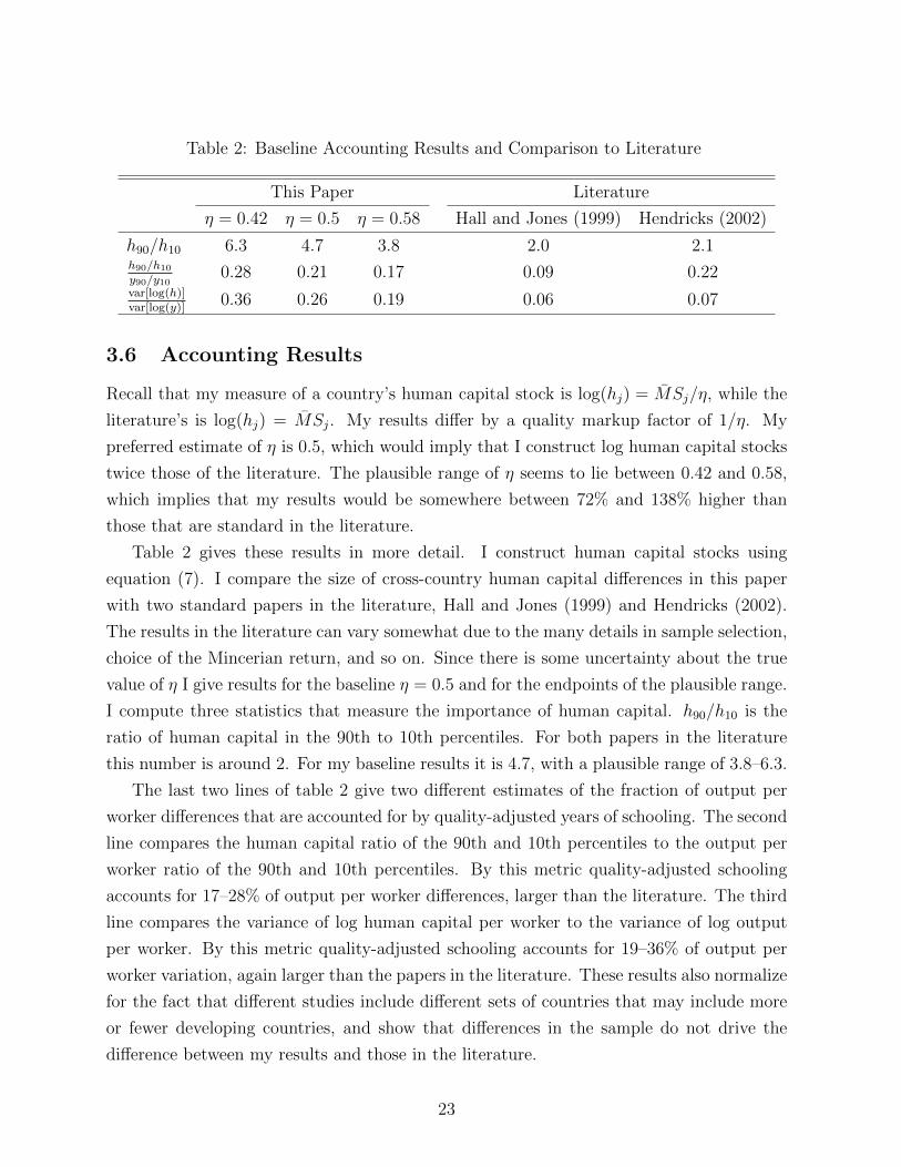
Table 2: Baseline Accounting Results and Comparison to Literature
This Paper Literature
η = 0.42 η = 0.5 η = 0.58 Hall and Jones (1999) Hendricks (2002)
h90/h10 6.3 4.7 3.8 2.0 2.1h90/h10y90/y10
0.28 0.21 0.17 0.09 0.22var[log(h)]var[log(y)]
0.36 0.26 0.19 0.06 0.07
3.6 Accounting Results
Recall that my measure of a country’s human capital stock is log(hj) = MSj/η, while the
literature’s is log(hj) = MSj. My results differ by a quality markup factor of 1/η. My
preferred estimate of η is 0.5, which would imply that I construct log human capital stocks
twice those of the literature. The plausible range of η seems to lie between 0.42 and 0.58,
which implies that my results would be somewhere between 72% and 138% higher than
those that are standard in the literature.
Table 2 gives these results in more detail. I construct human capital stocks using
equation (7). I compare the size of cross-country human capital differences in this paper
with two standard papers in the literature, Hall and Jones (1999) and Hendricks (2002).
The results in the literature can vary somewhat due to the many details in sample selection,
choice of the Mincerian return, and so on. Since there is some uncertainty about the true
value of η I give results for the baseline η = 0.5 and for the endpoints of the plausible range.
I compute three statistics that measure the importance of human capital. h90/h10 is the
ratio of human capital in the 90th to 10th percentiles. For both papers in the literature
this number is around 2. For my baseline results it is 4.7, with a plausible range of 3.8–6.3.
The last two lines of table 2 give two different estimates of the fraction of output per
worker differences that are accounted for by quality-adjusted years of schooling. The second
line compares the human capital ratio of the 90th and 10th percentiles to the output per
worker ratio of the 90th and 10th percentiles. By this metric quality-adjusted schooling
accounts for 17–28% of output per worker differences, larger than the literature. The third
line compares the variance of log human capital per worker to the variance of log output
per worker. By this metric quality-adjusted schooling accounts for 19–36% of output per
worker variation, again larger than the papers in the literature. These results also normalize
for the fact that different studies include different sets of countries that may include more
or fewer developing countries, and show that differences in the sample do not drive the
difference between my results and those in the literature.
23

Figure 6: Comparison of Accounting Results, Country-by-Country
0.5
1R
elat
ive
Hum
an C
apita
l, Li
tera
ture
0 .2 .4 .6 .8 1Relative Human Capital, Baseline
Hall/Jones (1999) Hendricks (2002)45−Degree Line
Figure 6 gives a country-by-country comparison of my results for human capital and the
literature’s. It plots estimated human capital from Hall and Jones (1999) and Hendricks
(2002) against my benchmark estimated human capital with η = 0.5. Human capital
is normalized by the level of the U.S. for both axes. The 45-degree line is included for
reference. For almost all countries in both papers in the literature the results are above the
45-degree line, indicating that the literature estimates smaller human capital per worker
gaps than I do.
My figures lie within the large bounds in the endogenous education quality literature.
For example Erosa, Koreshkova, and Restuccia (2010) compute that human capital variation
accounts for 13% of output per worker variation for two hypothetical economies differing
by a factor of 20 in income. On the other hand, Manuelli and Seshadri (2007) compute that
human capital variation accounts for 67% of output per worker variation between the top
and bottom deciles, although their model includes a broader notion of human capital than
I do here, with a large role for investments before schooling as well as on-the-job training.
My results are in the middle, and are quantitatively closer to those of Erosa, Koreshkova,
and Restuccia.
The main result of this paper comes from equations (7) and (8), along with the baseline
value of η = 0.5. Together they imply cross-country differences in education quality are
nearly as important as cross-country differences in years of schooling. Quality-adjusted
schooling accounts for 20% of cross-country output per worker differences, as opposed to
24

10% for years of schooling alone. Table 2 and figure 6 confirm this result by direct compar-
ison with two well-known sets of results in the existing literature.
4 Extensions
Section 3 established the baseline result of the paper, that quality-adjusted years of school-
ing account for 20% of cross-country output per worker differences, as opposed to 10%
for years of schooling alone. In this section I consider three extensions to the baseline
accounting framework. First, I allow for factors other than education quality to explain
cross-country schooling differences, and ask how this changes the baseline result. Second,
I allow for heterogeneity within a country in the rate of human capital formation per year
of schooling, and study the implications of this model for selection and the baseline re-
sults. Finally, I extend the model to allow for imperfect substitutability across skill types,
and show that this helps reconcile the patterns of returns to schooling for immigrants and
non-migrants.
4.1 Alternative Sources of Cross-Country Schooling Differences
In the baseline model η is estimated using the elasticity of schooling attainment with re-
spect to education quality. To this point the estimation assumes that all of the school
attainment differences between developed and developing countries can be explained by ed-
ucation quality differences. In this section I relax that assumption and show that it results
in a modest reduction in the development accounting results.
The equilibrium model of schooling suggests some potential alternative factors that
affect school choice. As a reminder, the model’s predicted equilibrium schooling for country
j is given by:
Sj =
[Qηj
Mj
]1/(1−η)
=
[Qηj
(rj − gj)(1 + λj)
]1/(1−η)
.
While education quality affects school choice, so do tuition costs, expected growth rates,
and interest rates.
The next step is to disentangle the relative contribution of education quality from these
other factors. The key information for this step comes from the returns to schooling of
non-migrants Mj. In equilibrium, workers equate the marginal benefit of schooling (higher
human capital) with the marginal cost (foregone wages and tuition); the marginal cost is
25

measured by Mj = (rj − gj)(1 + µj). The insight is that education quality affects school
choice differently from the other factors. Education quality raises the marginal benefit by
making each year more productive. Given that the marginal cost is the same, this induces
workers to go to school longer, until marginal benefits and marginal costs are again equated.
On the other hand, lower tuition reduces the marginal cost of schooling. Given that the
marginal benefit is the same, this induces workers to go to school longer, but it also lowers
the return to schooling Mj. Thus, the role of non-quality factors can be inferred by asking
whether Mj is generally lower for countries with higher school attainment.
The same insight applies to costs more generally defined, and even applies to frictions.
For example, suppose that workers’ optimal school choice is Sj years of schooling. However,
attending school requires paying tuition and foregoing income today in anticipation of higher
future earnings. The lack of well-functioning capital markets in developing countries may
make it impractical for families or students to borrow to finance schooling today. In this
case, average school attainment may be limited to S∗j < Sj. Given diminishing returns to
schooling, it necessarily follows that returns to schooling in this country are higher than
they otherwise would be. Again, the model suggests asking whether Mj is generally lower
for countries with higher school attainment.
Since Mincerian returns are noisy, I follow Bils and Klenow (2000) and use the trend
relationship between returns to schooling of non-migrants and schooling rather than indi-
vidual country observations. The estimated relationship is
log(Mj(S)) = b1 + b2 log(Sj) = −2.28− 0.073 log(Sj),
with standard errors 0.200 and 0.108. The fitted relationship has a negative but statistically
insignificant slope, indicating only modestly lower returns to schooling for non-migrants
and offering only weak support for the hypothesis that much of cross-country schooling
differences are explained by costs and frictions. Bils and Klenow estimate a much steeper
relationship
log(MBKj (S)) = b1 + b2 log(Sj) = −1.139− 0.58 log(Sj).
Their data includes several point estimates that have since been identified as potentially
noisy, and which were dropped from the Banerjee and Duflo (2005) data used here (see
Bennel (1996) for further discussion). Below I show the results that would prevail using
their much steeper fitted relationship.
Returns to schooling for non-migrants are generally lower in countries with higher school
26

attainment, which affects the interpretation of the relationship between years of schooling
and education quality. If I re-write equation (9) assuming that Mj = Mj(S) (instead of
Mj = M , as was assumed before) I find:
log (Sj) = c− b2
1− ηlog (Sj) +
η
1− ηlog(µjUS
)= c+
η
1− η + b2
log(µjUS
)where c again gathers together a number of terms that are constant. It is still sensible to
estimate the elasticity of school attainment with respect to education quality, but account-
ing for costs and frictions changes the interpretation of the elasticity. Only a portion is
causally attributed to education quality, while the rest is attributed to differences in costs
and frictions, as revealed through the fitted relationship between returns to schooling of
non-migrants and the average school attainment of the country. Finally, human capital can
be constructed as:
log(hj) =SjηMj(S).
Table 3 summarizes the development accounting results for the model with costs and
frictions. All of the results are based on the baseline estimated quantity-quality elasticity
of 1. The first column repeats the results for the frictionless model given in table 2. In this
interpretation η = 0.5, all of school differences are by assumption due to quality differences,
and human capital accounts for 21-26% of output per worker differences.
The remaining two columns interpret the quantity-quality elasticity differently in light of
the observation that on average highly educated countries have lower returns to schooling
for non-migrants. In the second column I use the Mj(S) estimated in this paper from
Banerjee and Duflo’s data. Returns to schooling for non-migrants are only modestly lower
in educated countries in their data. Because of this I infer that 86% of cross-country
differences in years of schooling are attributable to education quality, and that η is similar
to the baseline case. Then cross-country differences in human capital account for 18-21%
of cross-country differences in output per worker, slightly lower than in the baseline. The
MBKj (S) estimated by Bils and Klenow is much steeper. Returns to schooling for non-
migrants are much lower in educated countries. The third column shows that in this case
the correct inference is that most cross-country school differences are due to factors other
than education quality, and the estimated elasticity is quite low at η = 0.21. Despite
this, cross-country differences in human capital are larger, a factor of 6.7 between the 90th
27

Table 3: Robustness to Alternative Sources of School Attainment Dif-ferences
Baseline Allowing for Alternative Sources
Banerjee/Duflo Bils/Klenow
η 0.50 0.46 0.21
% S Attributed to Q 100% 86% 26%
h90/h10 4.7 4.1 6.7h90/h10y90/y10
0.21 0.18 0.30var[log(h)]var[log(y)]
0.26 0.21 0.40
Table notes: Baseline results are those from Table 2, attributing all ofcross-country schooling differences to education quality. The remaining columnsallow for alternative sources of cross-country schooling differences. Thequantitative role of alternative sources is estimated from returns to schooling ofnon-migrants in Banerjee and Duflo (2005) or Bils and Klenow (2000).
and 10th percentiles, and human capital accounts for 30-40% of cross-country output per
worker differences. This counterintuitive result obtains because Bils and Klenow estimate
an average return to schooling for non-migrants 50% higher than I do, which acts to raise
the importance of schooling.
The evidence from cross-country differences in returns to schooling for non-migrants
suggest a small role for costs and frictions in explaining cross-country schooling differences.
Alternatively, exogenous differences in the skill bias of technology provide a potential com-
peting explanation for cross-country schooling differences without implying counterfactually
large differences in Mincer rates of return across countries. However, papers in the liter-
ature typically assume the opposite causality, that exogenously higher schooling leads to
endogenous skill bias in innovation (Acemoglu 2002) or to the choice of more skill-biased
technologies among the set of existing technologies (Caselli and Coleman 2006). This paper
explains why such schooling differences may exist (as a result of education quality differ-
ences). Endogenous technology choice would provide an amplification mechanism that
interacts with the schooling differences caused by education quality.
4.2 Cognitive Ability Heterogeneity
The baseline model allows for cross-country variation in the rate of human capital forma-
tion per year of schooling, but no variation within countries. In this section I relax that
assumption and allow for within-country differences in the rate of human capital formation,
which I attribute to cognitive ability heterogeneity in the population, although education
28

quality heterogeneity is also plausible. I revisit the issue of selection and measured returns
to schooling in an environment where workers may also be selected on how well they learn.
I augment the human capital production function to allow for two explicit sources of
heterogeneity:
h(Sj, Qj, εkj , C
kj ) = εkj exp
[(SjQjC
kj )η
η
].
εkj is the more standard notion of ability, but could also measure characteristics such as
persistence or diligence. Ckj is cognitive ability, the characteristic that affects how much
human capital workers obtain in a given year of schooling.
The two types of ability affect school choices and wages differently. The optimal school
choice depends on cognitive ability but not non-cognitive ability,
Skj =
[(QjC
kj
)ηMj
]1/(1−η)
. (10)
Non-cognitive ability affects the intercept of log-wages, and will be captured by the fixed
effect γjUS. Cognitive ability affects the slope of log-wages with respect to schooling and is
captured by the return to schooling µjUS.
The discussion of selection in section 2.3 focused on the case where workers were selected
or differentially selected on εkj , their non-cognitive ability. A natural extension is to allow
for selection on cognitive ability. It follows from equation (10) that since the cognitively
able learn more in a year of schooling they will tend to go to school longer. Then the
degree of selection on cognitive ability can be inferred by comparing the school attainment
of immigrants to non-migrants.
Figure 7 plots the educational attainment of immigrants in my sample against the
educational attainment of non-migrants, taken from Barro and Lee (2001). Immigrants from
every country are positively selected on years of schooling. In some cases, this selection is
quite extreme: immigrants from Afghanistan, Nepal, Sierra Leone, and Sudan all have 13-14
years of schooling, while non-migrants in those countries have 1-2 years of schooling.18 Since
immigrants from most countries are positively selected on school attainment, I infer that
they are positively selected on cognitive ability. It then follows that the estimated returns
18There is a slight discontinuity since the data for immigrants measures schooling for workers, whileBarro and Lee’s data measures schooling in the population age 25 and over. Hence, the average Americanin my sample has 13.5 years of schooling, while Barro and Lee’s data report an American average of 12.2,indicating that Americans are “selected” by 1.3 years. Still, only Mexican immigrants are less selected.
29

Figure 7: Schooling of Immigrants and Non-Migrants
AFGETH
NPLSDNSLE
SENLBRMMRBGDPAK
HTI
UGA
CMR
GTM
KEN
GHA
HND
DZAIRN
IRQNIC
IDN
SLV
IND
BRA
EGYZWE
PRT
TUR
COL
DOM
JAMBOLSYR
VEN
CHN
LKA
PRYTHAGUY
CRIECU
MEX
JOR
KWT
ITACUBESP
URYPER
TTOYUG
PHL
CHLMYS
FJI
PAN
SGPFRATWN
GRC
ZAF
ARG
AUT
HUN
BEL
CYP
BRB
IRL
NLDGBRISR
BGR
HKG
ROMJPNGER
POL
FINDNK
KOR
CHEAUSCSK
CAN
SWE
NZLNOR
05
1015
Yea
rs o
f Sch
oolin
g, Im
mig
rant
s
0 5 10 15Years of Schooling, Non−Migrants
Data 45−Degree Line
to schooling of immigrants generally overstate the education quality of their source country,
since immigrants are a selected sample of those who gain most from a year of schooling.
Further, immigrants from developing countries are more selected on school attainment, so
I infer that they are more selected on cognitive ability, and that their estimated returns
to schooling overstate the education quality of their source country to a greater extent. In
this case, there are actually larger cross-country differences in education quality than what
I measured in section 2, and my development accounting results would be larger.
An alternative theory is that educational systems in developing countries are less effec-
tive at identifying and educating cognitively able students. In developed countries, educa-
tional attainment is based in large part on examinations of ability and merit, such as the
scholastic aptitude test (SAT) in the United States. But perhaps in developing countries
some other factor (such as political connections or family income) determines who is able
to attend school. In this case, the low measured returns to schooling for immigrants from
developing countries are a function of educating wealthy and politically connected students
rather than cognitively able students. My results count this as a form of (low) education
quality. This definition is somewhat more expansive than the usual one, which focuses on
factors such as training of teachers, availability of books, or class size; it is more in the
spirit of an inefficiency or misallocation in the education sector.
The fact that the more able go to school longer raises a second and distinct concern. This
framework captures the common concern of ability bias in measured returns to schooling:
30
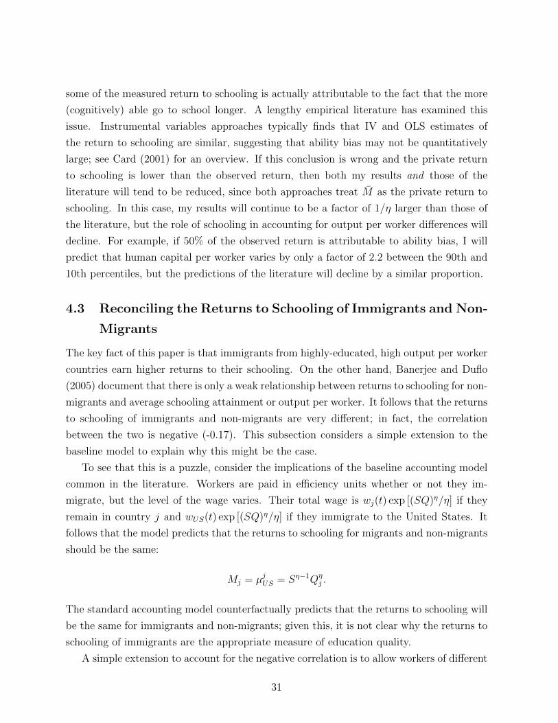
some of the measured return to schooling is actually attributable to the fact that the more
(cognitively) able go to school longer. A lengthy empirical literature has examined this
issue. Instrumental variables approaches typically finds that IV and OLS estimates of
the return to schooling are similar, suggesting that ability bias may not be quantitatively
large; see Card (2001) for an overview. If this conclusion is wrong and the private return
to schooling is lower than the observed return, then both my results and those of the
literature will tend to be reduced, since both approaches treat M as the private return to
schooling. In this case, my results will continue to be a factor of 1/η larger than those of
the literature, but the role of schooling in accounting for output per worker differences will
decline. For example, if 50% of the observed return is attributable to ability bias, I will
predict that human capital per worker varies by only a factor of 2.2 between the 90th and
10th percentiles, but the predictions of the literature will decline by a similar proportion.
4.3 Reconciling the Returns to Schooling of Immigrants and Non-
Migrants
The key fact of this paper is that immigrants from highly-educated, high output per worker
countries earn higher returns to their schooling. On the other hand, Banerjee and Duflo
(2005) document that there is only a weak relationship between returns to schooling for non-
migrants and average schooling attainment or output per worker. It follows that the returns
to schooling of immigrants and non-migrants are very different; in fact, the correlation
between the two is negative (-0.17). This subsection considers a simple extension to the
baseline model to explain why this might be the case.
To see that this is a puzzle, consider the implications of the baseline accounting model
common in the literature. Workers are paid in efficiency units whether or not they im-
migrate, but the level of the wage varies. Their total wage is wj(t) exp [(SQ)η/η] if they
remain in country j and wUS(t) exp [(SQ)η/η] if they immigrate to the United States. It
follows that the model predicts that the returns to schooling for migrants and non-migrants
should be the same:
Mj = µjUS = Sη−1Qηj .
The standard accounting model counterfactually predicts that the returns to schooling will
be the same for immigrants and non-migrants; given this, it is not clear why the returns to
schooling of immigrants are the appropriate measure of education quality.
A simple extension to account for the negative correlation is to allow workers of different
31

skill types to be imperfect substitutes. With imperfect substitutes, low education quality
in developing countries is offset by the lack of skilled labor, and the high education quality
in developed countries is offset by the abundance of skilled labor, so that the return to
schooling in the two countries is roughly the same. However, a worker who emigrates from
a developing country to the United States has low education quality and enters a labor
market where human capital is abundant, yielding a low return to schooling. Intuitively,
the reason to measure returns to schooling using immigrants is that the aggregate labor
market conditions for workers are held constant.
To formalize this intuition, I augment the aggregate production function to allow dif-
ferent skill types to be imperfect substitutes. It is important to be careful in defining skill
types. In standard models, workers are differentiated by their educational attainment: high
school versus college (Katz and Murphy 1992), or uneducated versus educated (Caselli and
Coleman 2006). In this model, workers can have the same educational attainment but very
different human capital levels if they have different education quality. I modify the standard
approach so that workers of different human capital levels are imperfect substitutes; this
allows me to preserve the assumption that all workers who can read earn the same wage,
regardless of how many years of schooling were needed to acquire literacy. Then if lj(h) is
the density of workers with human capital h, output is given by
Yj = AjKαj
[∫ h
1
(hlj(h))1−1/σ dh
]σ(1−α)/(σ−1)
where a lower bound of 1 is suggested by the human capital production function and the
upper bound is set to h. This equation yields the familiar relationship between the wage
premium for workers of two different human capital endowments,
wj(h)
wj(h′)=
[lj(h)
lj(h′)
]−1/σ (h
h′
)1−1/σ
.
The relative wage paid to workers with different human capital (and schooling) levels de-
pends on the relative supply of labor with those two types, unlike in the standard develop-
ment accounting framework.
The problem of the workers remains the same. At an interior solution workers must be
indifferent between obtaining different levels of schooling. In equilibrium, this indifference
condition implies that the returns to schooling of non-migrants are given by Mj = (rj −gj)(1+λj). However, the returns to schooling of immigrants are given by µjUS = MUS
Qj
QUS6=
32
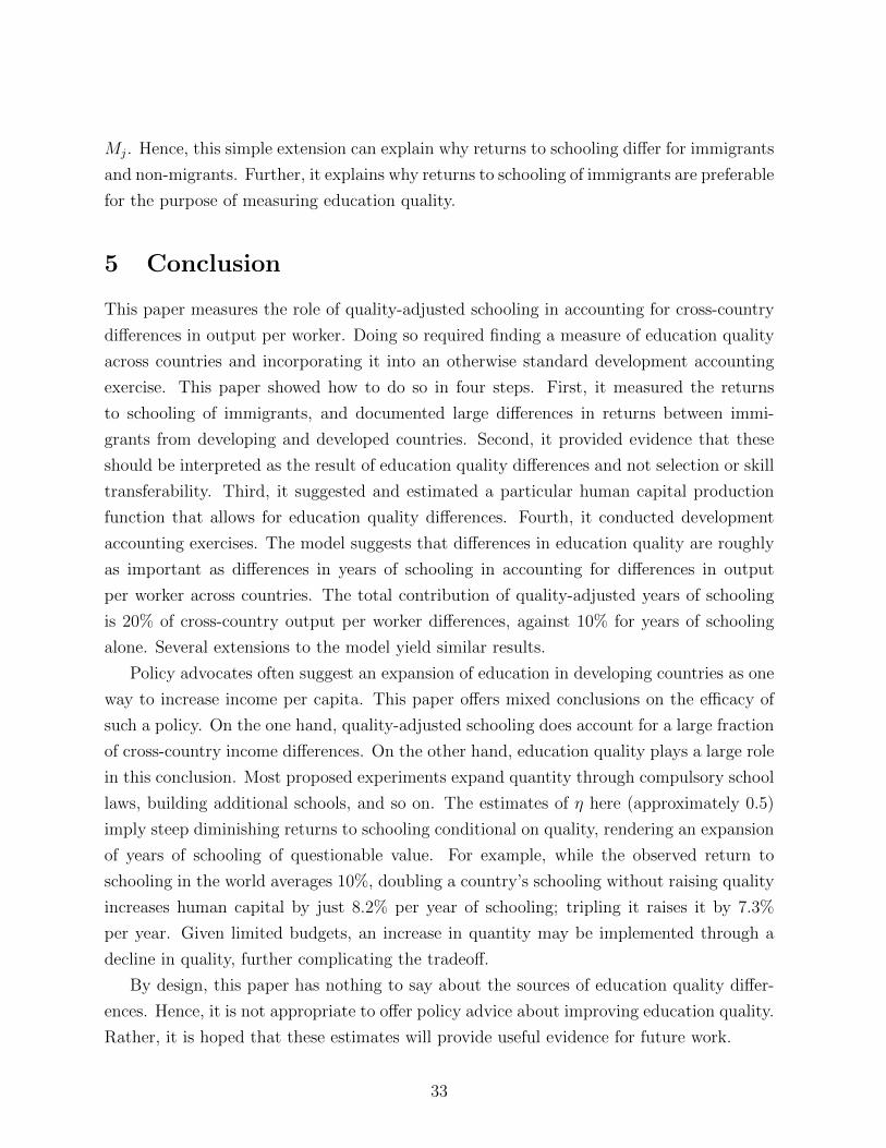
Mj. Hence, this simple extension can explain why returns to schooling differ for immigrants
and non-migrants. Further, it explains why returns to schooling of immigrants are preferable
for the purpose of measuring education quality.
5 Conclusion
This paper measures the role of quality-adjusted schooling in accounting for cross-country
differences in output per worker. Doing so required finding a measure of education quality
across countries and incorporating it into an otherwise standard development accounting
exercise. This paper showed how to do so in four steps. First, it measured the returns
to schooling of immigrants, and documented large differences in returns between immi-
grants from developing and developed countries. Second, it provided evidence that these
should be interpreted as the result of education quality differences and not selection or skill
transferability. Third, it suggested and estimated a particular human capital production
function that allows for education quality differences. Fourth, it conducted development
accounting exercises. The model suggests that differences in education quality are roughly
as important as differences in years of schooling in accounting for differences in output
per worker across countries. The total contribution of quality-adjusted years of schooling
is 20% of cross-country output per worker differences, against 10% for years of schooling
alone. Several extensions to the model yield similar results.
Policy advocates often suggest an expansion of education in developing countries as one
way to increase income per capita. This paper offers mixed conclusions on the efficacy of
such a policy. On the one hand, quality-adjusted schooling does account for a large fraction
of cross-country income differences. On the other hand, education quality plays a large role
in this conclusion. Most proposed experiments expand quantity through compulsory school
laws, building additional schools, and so on. The estimates of η here (approximately 0.5)
imply steep diminishing returns to schooling conditional on quality, rendering an expansion
of years of schooling of questionable value. For example, while the observed return to
schooling in the world averages 10%, doubling a country’s schooling without raising quality
increases human capital by just 8.2% per year of schooling; tripling it raises it by 7.3%
per year. Given limited budgets, an increase in quantity may be implemented through a
decline in quality, further complicating the tradeoff.
By design, this paper has nothing to say about the sources of education quality differ-
ences. Hence, it is not appropriate to offer policy advice about improving education quality.
Rather, it is hoped that these estimates will provide useful evidence for future work.
33

References
Acemoglu, D. (2002): “Change, Inequality, and the Labor Market,” Journal of Economic
Literature, 40(1), 7–72.
Antecol, H., D. A. Cobb-Clark, and S. J. Trejo (2003): “Immigration Policy and
the Skills of Immigrants to Australia, Canada, and the United States,” Journal of Human
Resources, 38(1), 192–218.
Banerjee, A. V., and E. Duflo (2005): “Growth Theory Through the Lens of De-
velopment Economics,” in Handbook of Economic Growth, ed. by P. Aghion, and S. N.
Durlauf, vol. 1A, chap. 7, pp. 473–554. Elsevier Science, North-Holland Publishers.
Barro, R. J. (1974): “Are Government Bonds Net Wealth?,” Journal of Political Econ-
omy, 82(6), 1095–1117.
Barro, R. J., and J.-W. Lee (2001): “International Data on Educational Attainment:
Updates and Implications,” Oxford Economic Papers, 53(3), 541–563.
Becker, G. S. (1964): Human Capital. University of Chicago Press, Chicago.
Ben-Porath, Y. (1967): “The Production of Human Capital and the Life Cycle of Earn-
ings,” Journal of Political Economy, 75(4), 352–265.
Bennel, P. (1996): “Rates of Return to Education: Does the Conventional Pattern Prevail
in Sub-Saharan Africa?,” World Development, 24(1), 183–199.
Bils, M., and P. J. Klenow (2000): “Does Schooling Cause Growth?,” American Eco-
nomic Review, 90(5), 1160–1183.
Borjas, G. J. (1999): “The Economic Analysis of Immigration,” in Handbook of Labor
Economics, ed. by O. Ashenfelter, and D. Card, vol. 3A, pp. 1697–1760. Elsevier Science,
North-Holland Publishers.
Bratsberg, B., and D. Terrell (2002): “School Quality and Returns to Education of
U.S. Immigrants,” Economic Inquiry, 40(2), 177–198.
Card, D. (2001): “Estimating the Return to Schooling: Progress on Some Persistent
Econometric Problems,” Econometrica, 69(5), 1127–1159.
34

Card, D., and A. B. Krueger (1992): “Does School Quality Matter? Returns to
Education and the Characteristics of Public Schools in the United States,” Journal of
Political Economy, 100(1), 1–40.
CareerOneStop (2010): “Licensed Occupations,” Available online at http:
//www.acinet.org/ACINET/LICENSEDOCCUPATIONS/lois_keyword.asp?nodeid=
16&by=keyword.
Case, A., and A. Deaton (1999): “School Inputs and Educational Outcomes in South
Africa,” Quarterly Journal of Economics, 114(3), 1047–1084.
Caselli, F. (2005): “Accounting for Cross-Country Income Differences,” in Handbook of
Economic Growth, ed. by P. Aghion, and S. N. Durlauf, vol. 1A, chap. 9, pp. 679–741.
Elsevier.
Caselli, F., and W. J. Coleman, II (2006): “The World Technology Frontier,” Amer-
ican Economic Review, 96(3), 499–522.
Cordoba, J. C., and M. Ripoll (2010): “What Explains Schooling Differences Across
Countries?,” mimeo, University of Pittsburgh.
Cortes, K. E. (2004): “Are Refugees Different From Economic Immigrants? Some Em-
pirical Evidence on the Heterogeneity of Immigrant Groups in the United States,” The
Review of Economics and Statistics, 86(2), 465–480.
Erosa, A., T. Koreshkova, and D. Restuccia (2010): “How Important is Human
Capital? A Quantitative Theory Assessment of World Income Inequality,” Review of
Economic Studies, forthcoming.
Friedberg, R. M. (1992): “The Labor Market Assimilation of Immigrants in the United
States: The Role of Age at Arrival,” mimeo, Brown University.
Hall, R. E., and C. I. Jones (1999): “Why Do Some Countries Produce So Much More
Output Per Worker Than Others?,” Quarterly Journal of Economics, 114(1), 83–116.
Hanushek, E., and L. Woessmann (2007): “The Role of School Improvement in Eco-
nomic Development,” PEPG 07-01.
(2011): “Sample Selectivity and the Validity of International Student Achievement
Tests in Economic Research,” Economics Letters, 110(2), 79–82.
35

Hanushek, E. A. (1995): “Interpreting Recent Research on Schooling in Developing
Countries,” World Bank Research Observer, 10(2), 227–246.
(2002): “Publicly Provided Education,” in Handbook of Public Economics, ed.
by A. J. Auerbach, and M. Feldstein, vol. 4, chap. 30, pp. 2045–2141. Elsevier Science,
North-Holland Publishers.
Hanushek, E. A., and D. D. Kimko (2000): “Schooling, Labor-Force Quality, and the
Growth of Nations,” American Economic Review, 90(5), 1184–1208.
Hanushek, E. A., V. Lavy, and K. Hitomi (2008): “Do Students Care About School
Quality? Determinants of Dropout Behavior in Developing Countries,” Journal of Hu-
man Capital, 2(1), 69–105.
Hanushek, E. A., and L. Woessmann (2009): “Do Better Schools Lead to More
Growth? Cognitive Skills, Economic Outcomes, and Causation,” NBER Working Pa-
per 14633.
Heckman, J., A. Layne-Farrar, and P. Todd (1996): “Human Capital Pricing Equa-
tions with an Application to Estimating the Effect of Schooling Quality on Earnings,”
The Review of Economics and Statistics, 78(4), 562–610.
Hendricks, L. (2002): “How Important Is Human Capital for Development? Evidence
from Immigrant Earnings,” American Economic Review, 92(1), 198–219.
Heston, A., R. Summers, and B. Aten (2009): Penn World Table Version 6.3. Center
for International Comparisons of Production, Income and Prices at the University of
Pennsylvania.
Jasso, G., D. S. Massey, M. R. Rosenzweig, and J. P. Smith (2000): “The New
Immigrant Survey Pilot (NIS-P): Overview and New Findings About U.S. Legal Immi-
grants at Admission,” Demography, 37(1), 127–138.
Katz, L. F., and K. M. Murphy (1992): “Changes in Relative Wages, 1963-1987:
Supply and Demand Factors,” The Quarterly Journal of Economics, 107(1), 35–78.
Manuelli, R. E., and A. Seshadri (2007): “Human Capital and the Wealth of Nations,”
Mimeo, University of Wisconsin - Madison.
Mincer, J. (1958): “Investment in Human Capital and Personal Income Distribution,”
Journal of Political Economy, 66(4), 281–302.
36

Minnesota Population Center (2010): “Integrated Public Use Microdata Series In-
ternational: Version 6. [Machine-readable database].,” Minneapolis: University of Min-
nesota., http://www.ipums.org.
Mortland, C. A. (1996): “Khmer,” in Refugees in American in the 1990s: A Reference
Handbook, ed. by D. W. Haines, chap. 11, pp. 232–258. Greenwood Press.
Psacharopoulos, G., and H. A. Patrinos (2004): “Returns to Investment in Educa-
tion: A Further Update,” Education Economics, 12(2), 111–134.
Ruggles, S., J. T. Alexander, K. Genadek, R. Goeken, M. B. Schroeder,
and M. Sobek (2010): “Integrated Public Use Microdata Series: Version 5.0 [Machine-
readable database],” Minneapolis: University of Minnesota.
Tamura, R. (2001): “Teachers, Growth, and Convergence,” Journal of Political Economy,
109, 1021–1059.
United States Department of State and United States Department of Home-
land Security and United States Department of Health and Human Ser-
vices (2009): Proposed Refugee Admissions for Fiscal Year 2009: Report to the Congress.
U.S. Immigration and Naturalization Service (1980-2000): Statistical Yearbook of
the Immigration and Naturalization Service. U.S. Government Printing Office, Washing-
ton, D.C.
You, H. M. (2008): “The Contribution of Rising School Quality to U.S. Economic
Growth,” mimeo, University at Buffalo, SUNY.
37

A Identification of Parameters for Immigrants’ Wages
The baseline regression of equation (1) omits a number of additional factors that are often
considered of interest in the broader immigration literature. In particular previous work
has argued for a role for assimilation and the age at arrival of immigrants (Friedberg 1992).
A more general model that allows for these factors will make several parameters of the wage
equation unidentified, but the country-specific return to schooling remains identified. To see
this, consider an extension of the baseline model along lines suggested in the immigration
literature:
log(W j,kUS) = bj + µjUSS
j,kUS + βXj,k
US + γCj,kUS + δY rsj,kUS + φArrAgej,kUS + εj,kUS (11)
where Cj,kUS is the cohort (year) of immigration for immigrant k from country j, Y rsj,kUS is the
years that immigrant has spent in the United States, and ArrAgej,kUS is their age at arrival.
While the baseline model allows for cohort fixed effects, log-linearity in cohort simplifies
the exposition.
The standard problem with this specification is that there are linear dependencies among
the right-hand side variables (Borjas 1999). In particular, Cj,kUS + Y rsj,kUS = 2000 since all
immigrants are observed in 2000. Substitution yields
log(W j,kUS) = bj + 2000δ + µjUSS
j,kUS + βXj,k
US + (γ − δ)Cj,kl + φArrAgej,kUS + εj,kUS. (12)
The true cohort and assimilation effects cannot be identified without pooling census years,
but this fact does not affect the measured returns to schooling. Among immigrants, there
is also a linear dependency between arrival age, cohort, and age or potential experience.
However, as noted in Friedberg (1992), it is possible to estimate age at arrival effects by
pooling immigrants with natives and assuming that the return to age or experience is the
same for both. Results for such a regression (available upon request) are similar to the
baseline.
B Estimated Returns to Schooling of Immigrants
Table 4: Estimated Returns to Schooling of Immigrants
Country Returns S.E. Obs
Tonga -0.003 0.068 100
Continued on Next Page
38

Table 4: Estimated Returns to Schooling of Immigrants
Country Returns S.E. Obs
Albania 0.000 0.038 324
Macedonia, FYR 0.005 0.058 121
Azores 0.009 0.061 89
Lao PDR 0.010 0.011 1344
Nepal 0.012 0.058 89
Cape Verde 0.013 0.040 222
Cambodia 0.017 0.015 898
Kosovo 0.018 0.075 41
Mexico 0.018 0.002 67026
Honduras 0.019 0.011 2604
Bosnia and Herzegovina 0.019 0.022 1130
Antigua and Barbuda 0.020 0.082 118
El Salvador 0.021 0.006 7557
Guatemala 0.021 0.008 4701
Somalia 0.021 0.033 170
Sierra Leone 0.022 0.055 217
Portugal 0.023 0.017 1017
Serbia 0.023 0.064 76
Sudan 0.024 0.053 115
Dominican Republic 0.025 0.009 4210
Bolivia 0.026 0.037 394
Vietnam 0.028 0.006 7720
Ecuador 0.028 0.012 2165
Eritrea 0.028 0.052 143
Cuba 0.028 0.010 4551
Armenia 0.028 0.038 308
Iraq 0.030 0.021 545
Nicaragua 0.030 0.014 1672
Liberia 0.035 0.044 333
Belize 0.035 0.048 211
Jordan 0.035 0.054 174
Peru 0.036 0.015 2393
Costa Rica 0.036 0.025 471
Korea, Rep. 0.037 0.034 583
Yugoslavia 0.037 0.029 448
Uzbekistan 0.037 0.070 157
Thailand 0.038 0.021 757
Colombia 0.040 0.010 3520
Continued on Next Page
39

Table 4: Estimated Returns to Schooling of Immigrants
Country Returns S.E. Obs
Yemen, Rep. 0.040 0.044 89
Haiti 0.041 0.011 3717
Uganda 0.041 0.079 102
Poland 0.042 0.013 3398
Senegal 0.045 0.057 87
Bangladesh 0.045 0.022 615
Ethiopia 0.045 0.031 564
Syrian Arab Republic 0.046 0.033 264
Samoa 0.047 0.066 81
Moldova 0.050 0.059 171
Cyprus 0.052 0.094 36
Nigeria 0.053 0.022 1062
Croatia 0.053 0.046 208
Paraguay 0.054 0.081 60
Latvia 0.054 0.087 93
Ghana 0.055 0.028 720
Spain 0.055 0.026 423
Dominica 0.056 0.065 129
Saudi Arabia 0.056 0.090 64
Azerbaijan 0.057 0.069 123
Grenada 0.057 0.058 191
Myanmar 0.057 0.031 305
Trinidad and Tobago 0.057 0.023 1353
Puerto Rico 0.058 0.009 4671
Czech Republic 0.058 0.083 103
Finland 0.058 0.090 119
Egypt, Arab Rep. 0.058 0.029 742
Pakistan 0.059 0.016 1312
Brazil 0.062 0.015 1597
Bulgaria 0.062 0.042 305
Cameroon 0.062 0.092 74
Indonesia 0.063 0.038 368
Guyana 0.063 0.017 1799
Algeria 0.063 0.064 85
Austria 0.064 0.060 132
Czechoslovakia 0.064 0.065 148
Venezuela, RB 0.065 0.025 608
Philippines 0.065 0.008 12066
Continued on Next Page
40

Table 4: Estimated Returns to Schooling of Immigrants
Country Returns S.E. Obs
Bahamas, The 0.067 0.077 114
Romania 0.067 0.022 1067
Turkey 0.068 0.029 415
Italy 0.068 0.018 998
Belarus 0.070 0.048 315
Jamaica 0.070 0.013 4348
Afghanistan 0.070 0.043 218
St. Lucia 0.071 0.100 104
Ukraine 0.071 0.019 1922
Georgia 0.072 0.088 67
Panama 0.073 0.034 561
Greece 0.075 0.030 460
China 0.075 0.005 7445
Chile 0.075 0.030 530
Fiji 0.075 0.048 280
Sri Lanka 0.076 0.045 249
Lithuania 0.078 0.083 109
Iran, Islamic Rep. 0.079 0.021 1344
India 0.079 0.008 6255
Barbados 0.080 0.046 388
Argentina 0.081 0.024 725
Kenya 0.083 0.049 254
Ireland 0.083 0.034 690
Taiwan 0.086 0.020 1559
France 0.088 0.026 664
Malaysia 0.089 0.032 306
St. Vincent and the Grenadines 0.089 0.059 138
Morocco 0.090 0.044 254
Lebanon 0.091 0.033 414
St. Kitts and Nevis 0.092 0.114 89
Hong Kong, China 0.092 0.019 1102
Israel 0.093 0.029 543
Uruguay 0.093 0.056 168
Slovak Republic 0.094 0.097 95
Denmark 0.094 0.064 147
Singapore 0.094 0.072 110
Bermuda 0.096 0.101 55
Zimbabwe 0.097 0.089 89
Continued on Next Page
41

Table 4: Estimated Returns to Schooling of Immigrants
Country Returns S.E. Obs
New Zealand 0.101 0.061 195
Australia 0.101 0.041 460
Canada 0.102 0.014 3783
Germany 0.106 0.016 2452
Belgium 0.108 0.058 125
United Kingdom 0.108 0.014 4042
South Africa 0.110 0.037 495
United States 0.111 0.001 4.1e+06
Netherlands 0.111 0.044 329
Norway 0.112 0.073 123
Hungary 0.114 0.046 271
Kuwait 0.114 0.107 42
Sweden 0.116 0.055 226
Japan 0.120 0.018 2188
Switzerland 0.126 0.063 188
Tanzania 0.131 0.097 73
Note: Country is the country name as it is recorded in the census files. Returns are the
log-wage returns to schooling. S.E. is the standard error of the returns. Obs is the number
of observations in the 2000 5% PUMS meeting the sample restrictions.
42