Educational opportunity in early and middle childhood: Variation by place and age

I use standardized test scores from roughly 45 million students to describe the temporal

structure of educational opportunity in over 11,000 school districts—almost every district in

the US. For each school district, I construct two measures: the average academic

performance of students in grade 3 and the within-cohort growth in test scores from grade

3 to 8. I argue that third grade average test scores can be thought of as measures of the

average extent of educational opportunities available to students in a community prior to

age 9. Growth rates in average scores from grade 3 to 8 can be thought of as reflecting

educational opportunities available to children in a school district between the ages of 9

and 14.

I document considerable variation among school districts in both average third grade

scores and test score growth rates. Importantly, the two measures are uncorrelated,

indicating that the characteristics of communities that provide high levels of early childhood

educational opportunity are not the same as those that provide high opportunities for

growth from third to eighth grade. This suggests that the role of schools in shaping

educational opportunity varies across school districts. Moreover, the variation among

districts in the two temporal opportunity dimensions implies that strategies to improve

educational opportunity may need to target different age groups in different places. One

additional implication of the low correlation between growth rates and average third grade

scores is that measures of average test scores are likely very poor measures of school

effectiveness. The growth measure I construct does not isolate the contribution of schools

to children’s academic skills, but is likely closer to a measure of school effectiveness than

are measures of average test scores.

ABSTRACTAUTHORS

VERSION

December 2017

Suggested citation: Reardon, S.F. (2017). TEducational opportunity in early and middle childhood: Variation by place and age (CEPA Working Paper No.17-12). Retrieved from Stanford Center for Education Policy Analysis: http://cepa.stanford.edu/wp17-12

CEPA Working Paper No. 17-12

Sean F. ReardonStanford University

Educational opportunity in early and middle childhood:

Variation by place and age

sean f. reardon Stanford University

Discussion Draft: December 4, 2017

This draft is circulated for discussion and is not finalized. Please share your comments and feedback with me at sean.reardon@stanford.edu. The research described here was supported by grants from the Institute of Education Sciences (R305D110018), the Spencer Foundation (Award #201500058), the William T. Grant Foundation (Award #186173), the Bill and Melinda Gates Foundation, and the Overdeck Family Foundation. The paper would not have been possible without the assistance of Ross Santy, Michael Hawes, and Marilyn Seastrom, who facilitated access to the EDFacts data. This paper benefitted substantially from ongoing collaboration with Andrew Ho, Erin Fahle, and Ben Shear and from the research assistance of Joseph Van Matre and Richard DiSalvo. Some of the data used in this paper were provided by the National Center for Education Statistics (NCES). The opinions expressed here are my own and do not represent views of NCES, the Institute of Education Sciences, the U.S. Department of Education, the Spencer Foundation, the William T. Grant Foundation, the Bill and Melinda Gates Foundation, or the Overdeck Family Foundation. Direct correspondence and comments to Sean F. Reardon, sean.reardon@stanford.edu, 520 CERAS Building #526, Stanford University, Stanford, CA 94305.

Educational opportunity in early and middle childhood:

Variation by place and age

Abstract

I use standardized test scores from roughly 45 million students to describe the temporal

structure of educational opportunity in over 11,000 school districts—almost every district in the US. For

each school district, I construct two measures: the average academic performance of students in grade 3

and the within-cohort growth in test scores from grade 3 to 8. I argue that third grade average test scores

can be thought of as measures of the average extent of educational opportunities available to students in

a community prior to age 9. Growth rates in average scores from grade 3 to 8 can be thought of as

reflecting educational opportunities available to children in a school district between the ages of 9 and

14.

I document considerable variation among school districts in both average third grade scores and

test score growth rates. Importantly, the two measures are uncorrelated, indicating that the

characteristics of communities that provide high levels of early childhood educational opportunity are not

the same as those that provide high opportunities for growth from third to eighth grade. This suggests

that the role of schools in shaping educational opportunity varies across school districts. Moreover, the

variation among districts in the two temporal opportunity dimensions implies that strategies to improve

educational opportunity may need to target different age groups in different places. One additional

implication of the low correlation between growth rates and average third grade scores is that measures

of average test scores are likely very poor measures of school effectiveness. The growth measure I

construct does not isolate the contribution of schools to children’s academic skills, but is likely closer to a

measure of school effectiveness than are measures of average test scores.

1

Educational opportunity in early and middle childhood:

Variation by place and age

Introduction

Are public schools in the US engines of mobility or agents of inequality? Can schools in low-

income communities provide a pathway out of poverty, or are the constraints of poverty too great for

schools to overcome? Such questions are at the heart of debates about the role of education in social

mobility in the US. Despite decades of research, we still lack clear answers, however.

In this paper I provide new evidence to inform these debates. This new evidence suggests that

there is no clear answer to the question in part because the role of schooling in shaping educational

opportunity varies substantially across places. Early childhood conditions more important in some places;

educational opportunities during the elementary and middle school years appear more important in

others.

In the first part of the paper, I use standardized test scores from roughly 45 million students to

construct measures of the temporal structure of educational opportunity in over 11,000 school districts—

almost every district in the US. The data span the school years 2008-09 through 2014-15. For each school

district, I construct two measures: the average academic performance of students in grade 3 and the

within-cohort growth in test scores from grade 3 to 8. I argue that average test scores in a school district

can be thought of as reflecting the average cumulative set of educational opportunities children in a

community have had up to the time when they take a test.

Given this, the average scores in grade 3 can be thought of as measures of the average extent of

“early educational opportunities” (reflecting opportunities from birth to age 9) available to children in a

school district. Prior research suggest that these early opportunities are strongly related to the average

socioeconomic resources available in children’s families in the district. They may also depend on other

2

characteristics of the community, including neighborhood conditions, the availability of high-quality child

care and pre-school programs, and the quality of schools in grades K-3.

The growth in average test scores from grades 3 to 8 can likewise be thought of as a measure of

the average extent of “middle childhood educational opportunities” available to children in a school

district while they are roughly age 9 to 14. Given the prominence of schooling in children’s lives at these

ages, these middle childhood opportunities may depend in large part on the quality of the local

elementary and middle schools. They may also depend on average family resources, of course, as well as

other local conditions, including neighborhood characteristics and the availability of afterschool

programs.

Given these two measures, average scores in eighth grade are then understood to reflect the

cumulative set of early and middle grade educational opportunities in a school district. The

decomposition of eighth grade average scores into the two components, reflecting early opportunity and

middle grades opportunity, provides insight into the temporal structure of educational opportunity. The

availability of these two measures for over 11,000 school districts yields unprecedented insight into the

geographic and temporal structure of childhood educational opportunity in the U.S.

In the second part of the paper, I describe both the relationship between these two measures

and their association with socioeconomic characteristics of school districts. I find that the two measures

are largely uncorrelated; early and middle-grades opportunities appear to be distinct and separable

dimensions of local educational opportunity structures. Among districts with a given level of average test

scores in third grade, there is wide variation in growth in average scores from third to eighth grade.

Moreover, although both dimensions of opportunity are positively associated with district socioeconomic

conditions, the correlation is much weaker for the middle grades growth dimension. There are many low-

income school districts with relatively high measures of growth and many affluent districts with relatively

low growth. Finally, I also examine the temporal opportunity structure separately by race/ethnic group

3

and for poor and non-poor students.

The descriptive evidence I present is relevant to several scholarly and policy discussions. First, it

suggests that the role of schooling (and factors that shape children’s academic progress during the years

they are in school) in shaping educational opportunity (and perhaps social mobility) varies across school

districts. The answer to the question of whether schools exacerbate or ameliorate socioeconomic

inequality may be “it depends on where you are.” Second, the variation among districts in the two

temporal opportunity dimensions implies that strategies to improve educational opportunity may need to

target different age groups in different places. Third, one implication of the low correlation between

growth rates and average third grade scores is that measures of average test scores are likely very poor

measures of school quality. The growth measure I construct does not isolate the contribution of schools

to children’s academic skills, but is likely closer to a measure of school effectiveness than are measures of

average test scores.

Background

Educational outcomes vary widely by socioeconomic status and race/ethnicity in the US. Children

in high-income families, and those whose parent or parents have college degrees, systematically score

higher on standardized tests and are more likely to attend and graduate from college than lower-income

students and students whose parents did not attend college. Similar disparities are evident between

White and Asian students and Black, Hispanic, and Native American Students (Chetty et al. 2017; Reardon

2011; Reardon, Robinson-Cimpian and Weathers 2015; Sirin 2005; Ziol-Guest and Lee 2016). This

inequality in average group outcomes is prima facie evidence of systematic between-group differences in

opportunity. But disparities in outcomes alone do not indicate the ways in which opportunities differ, nor

the developmental stage when they are most salient. In particular, they do not tell us to what extent

schools—and inequalities in schools—are to blame for these patterns. Here I briefly discuss two strands

4

of scholarship that are relevant to this question: debates about the role of schools in shaping inequality,

and evidence regarding place-based opportunity structures.

Schools as “the great equalizer” in the United States

The debate regarding schools’ role in providing educational opportunity and facilitating social

mobility has a long history, particularly among sociologists. Three dominant arguments shape the debate.

One position holds that schools reduce inequality of opportunity. The stark inequality in children’s family

backgrounds creates large differences in children’s opportunities to learn, but school environments—in

this argument—are less unequal than children’s home environments. Evidence for this view comes from

research showing, for example, that racial or socioeconomic achievement gaps widen in the summer

when children are not in school, but narrow (or at least do not grow) when children are in school

(Alexander, Entwisle and Olson 2001; Alexander, Entwisle and Olson 2007; Downey and Condron 2016;

Downey, Hippel and Broh 2004). This evidence is sensitive to the scale used to measure academic

performance, however; not all studies show these same patterns (von Hippel, Workman and Downey

2017). Additional support for this argument comes from studies showing that poor children benefit more

from expanded time in school (via universal preschool enrollment, universal kindergarten, full-day

kindergarten, and extended school days) than do non-poor children (Raudenbush and Eschmann 2015).

A second position is that schools have relatively little effect on the inequality of educational

outcomes; family background is a far stronger force than schooling. In this view, most educational

inequality is produced early in children’s lives and by differences in family resources. This was the

conclusion of the 1966 Coleman Report, and was, to some extent, the argument of Jencks and his

colleagues (Coleman et al. 1966; Jencks 1972). Additional evidence for this view comes from studies that

find that socioeconomic or racial achievement gaps are large when children arrive in formal schooling in

kindergarten, and do not change appreciably during the schooling years (Reardon 2011; Reardon,

5

Robinson-Cimpian and Weathers 2015).

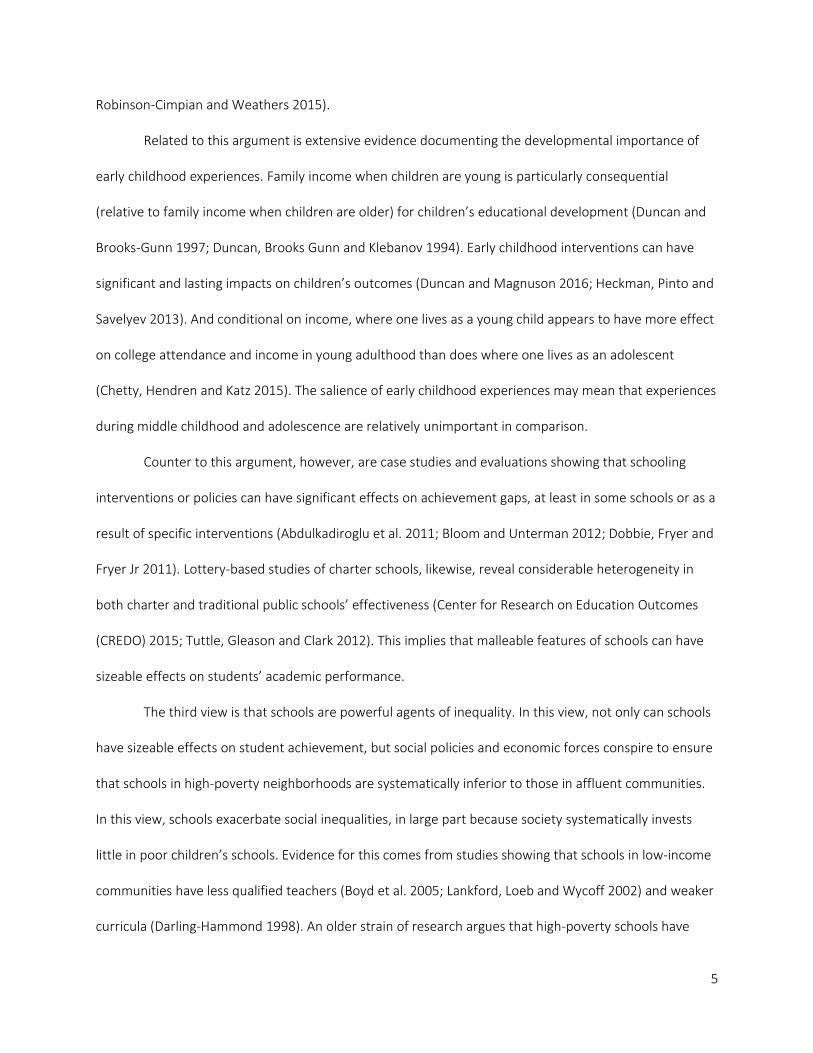
Related to this argument is extensive evidence documenting the developmental importance of

early childhood experiences. Family income when children are young is particularly consequential

(relative to family income when children are older) for children’s educational development (Duncan and

Brooks-Gunn 1997; Duncan, Brooks Gunn and Klebanov 1994). Early childhood interventions can have

significant and lasting impacts on children’s outcomes (Duncan and Magnuson 2016; Heckman, Pinto and

Savelyev 2013). And conditional on income, where one lives as a young child appears to have more effect

on college attendance and income in young adulthood than does where one lives as an adolescent

(Chetty, Hendren and Katz 2015). The salience of early childhood experiences may mean that experiences

during middle childhood and adolescence are relatively unimportant in comparison.

Counter to this argument, however, are case studies and evaluations showing that schooling

interventions or policies can have significant effects on achievement gaps, at least in some schools or as a

result of specific interventions (Abdulkadiroglu et al. 2011; Bloom and Unterman 2012; Dobbie, Fryer and

Fryer Jr 2011). Lottery-based studies of charter schools, likewise, reveal considerable heterogeneity in

both charter and traditional public schools’ effectiveness (Center for Research on Education Outcomes

(CREDO) 2015; Tuttle, Gleason and Clark 2012). This implies that malleable features of schools can have

sizeable effects on students’ academic performance.

The third view is that schools are powerful agents of inequality. In this view, not only can schools

have sizeable effects on student achievement, but social policies and economic forces conspire to ensure

that schools in high-poverty neighborhoods are systematically inferior to those in affluent communities.

In this view, schools exacerbate social inequalities, in large part because society systematically invests

little in poor children’s schools. Evidence for this comes from studies showing that schools in low-income

communities have less qualified teachers (Boyd et al. 2005; Lankford, Loeb and Wycoff 2002) and weaker

curricula (Darling-Hammond 1998). An older strain of research argues that high-poverty schools have

6

systematically fewer financial resources (see, for example, Kozol 1967; Kozol 1991), though in many

states this is no longer true (at least in terms of average per-pupil financial resources). An alternate, neo-

Marxist version of this argument holds that capitalism requires an unequal schooling system in order to

prepare students of different class background for their future roles in a capitalist economy (Bowles and

Gintis 1976).

Each of these arguments has both supporting and countervailing evidence. This is because there

is some truth to each of them, and because the role of schooling varies across place.

Geographic variation in educational opportunity

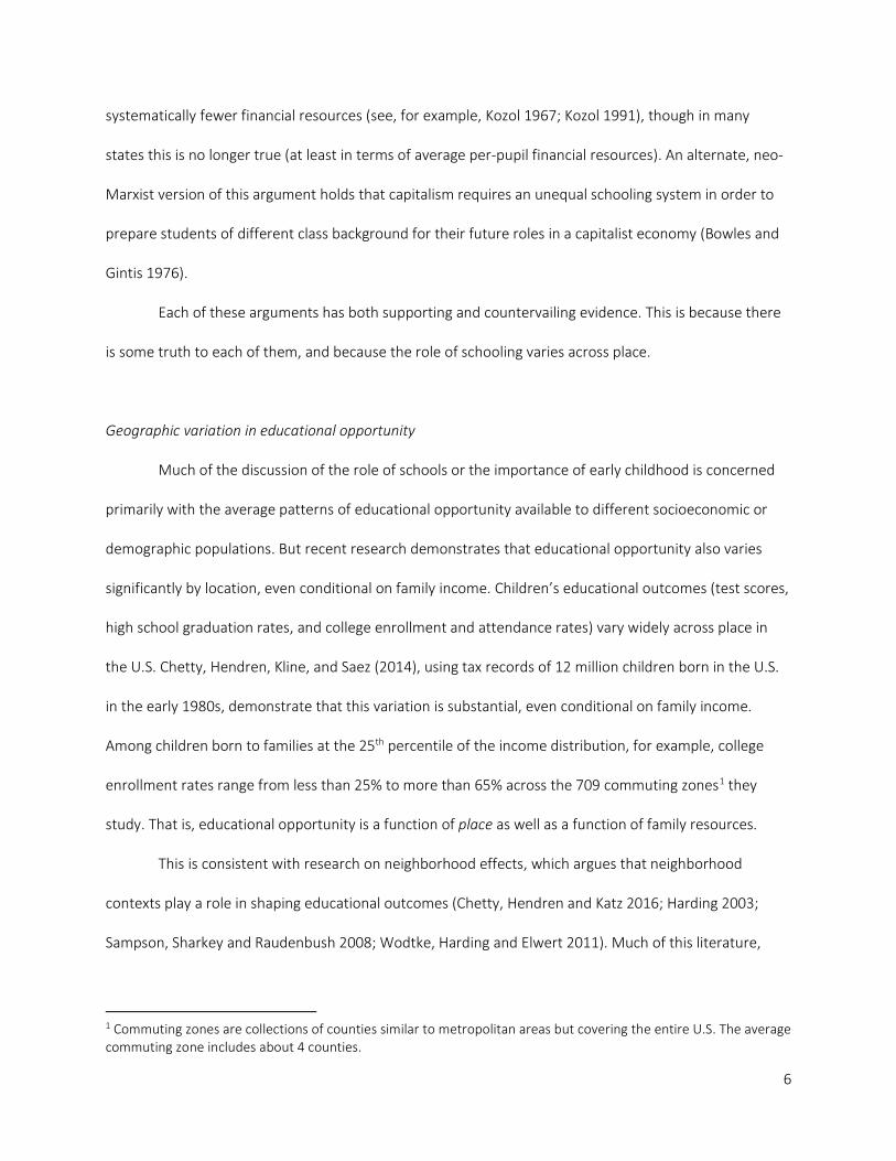
Much of the discussion of the role of schools or the importance of early childhood is concerned

primarily with the average patterns of educational opportunity available to different socioeconomic or

demographic populations. But recent research demonstrates that educational opportunity also varies

significantly by location, even conditional on family income. Children’s educational outcomes (test scores,

high school graduation rates, and college enrollment and attendance rates) vary widely across place in

the U.S. Chetty, Hendren, Kline, and Saez (2014), using tax records of 12 million children born in the U.S.

in the early 1980s, demonstrate that this variation is substantial, even conditional on family income.

Among children born to families at the 25th percentile of the income distribution, for example, college

enrollment rates range from less than 25% to more than 65% across the 709 commuting zones1 they

study. That is, educational opportunity is a function of place as well as a function of family resources.

This is consistent with research on neighborhood effects, which argues that neighborhood

contexts play a role in shaping educational outcomes (Chetty, Hendren and Katz 2016; Harding 2003;

Sampson, Sharkey and Raudenbush 2008; Wodtke, Harding and Elwert 2011). Much of this literature,

1 Commuting zones are collections of counties similar to metropolitan areas but covering the entire U.S. The average commuting zone includes about 4 counties.

7

however, focuses on the effects of neighborhood economic conditions; research has been less successful

at identifying the mechanisms through which neighborhood contexts and community institutions shape

educational opportunity. Chetty et al (2014) note that upward economic mobility of children born to low-

income families is lower in places with lower test scores and in more segregated places. Both of these are

consistent with a story in which the quality of local schools shapes opportunities for mobility: in

segregated areas, poor children are more concentrated in a subset of high-poverty schools; these schools

may be lower in quality, leading to lower test scores, which reduce future educational opportunities and

may be reflected in lower wages. But the evidence is far from definitive. Indeed, in another paper Chetty

and colleagues show that children’s neighborhood contexts when they are young are more influential

than their neighborhood conditions after age 10, a finding that suggests schools may not play a central

role in shaping mobility (Chetty, Hendren and Katz 2015).

In short, the evidence is increasingly clear that educational opportunity and social mobility vary

spatially. Less clear, however, is the role of schooling in shaping those patterns. Local contexts shape

academic skills and human capital, but how? In this paper, I provide evidence to help answer that

question, by describing evidence of the timing of these effects. By measuring average academic skills at

different ages in each school district, I provide information on how educational opportunity varies by age

across communities.

Temporal patterns of educational opportunity

Suppose we characterized each community on two dimensions of opportunity: opportunities

available to children in early childhood and opportunities available during their middle childhood. Early

opportunities might depend on experiences that children have in their homes, in child care and in

preschool. These will be strongly influenced by the average family resources in a community (income,

social capital, educational attainment), but may also depend on neighborhood conditions and local

8

context. For example, two equally poor communities may differ in the extent to which children are

exposed to lead paint or other environmental toxins. Two equally affluent communities may differ in the

quality of available pre-school programs. Middle-childhood opportunities may depend substantially on

children’s schooling experiences and the quality of the local schools, but also may be shaped by family

resources and neighborhood conditions, the availability of after school activities, neighborhood safety,

and so on.

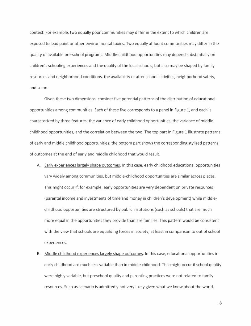
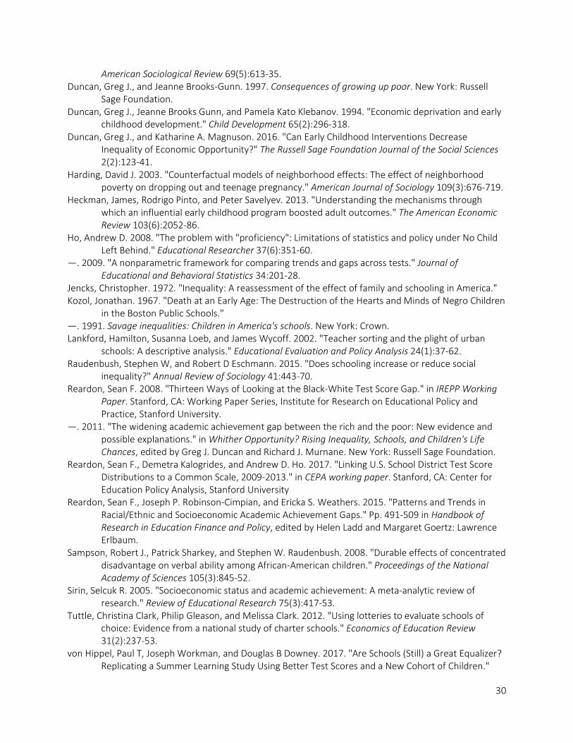
Given these two dimensions, consider five potential patterns of the distribution of educational

opportunities among communities. Each of these five corresponds to a panel in Figure 1, and each is

characterized by three features: the variance of early childhood opportunities, the variance of middle

childhood opportunities, and the correlation between the two. The top part in Figure 1 illustrate patterns

of early and middle childhood opportunities; the bottom part shows the corresponding stylized patterns

of outcomes at the end of early and middle childhood that would result.

A. Early experiences largely shape outcomes. In this case, early childhood educational opportunities

vary widely among communities, but middle-childhood opportunities are similar across places.

This might occur if, for example, early opportunities are very dependent on private resources

(parental income and investments of time and money in children’s development) while middle-

childhood opportunities are structured by public institutions (such as schools) that are much

more equal in the opportunities they provide than are families. This pattern would be consistent

with the view that schools are equalizing forces in society, at least in comparison to out of school

experiences.

B. Middle childhood experiences largely shape outcomes. In this case, educational opportunities in

early childhood are much less variable than in middle childhood. This might occur if school quality

were highly variable, but preschool quality and parenting practices were not related to family

resources. Such as scenario is admittedly not very likely given what we know about the world.

9

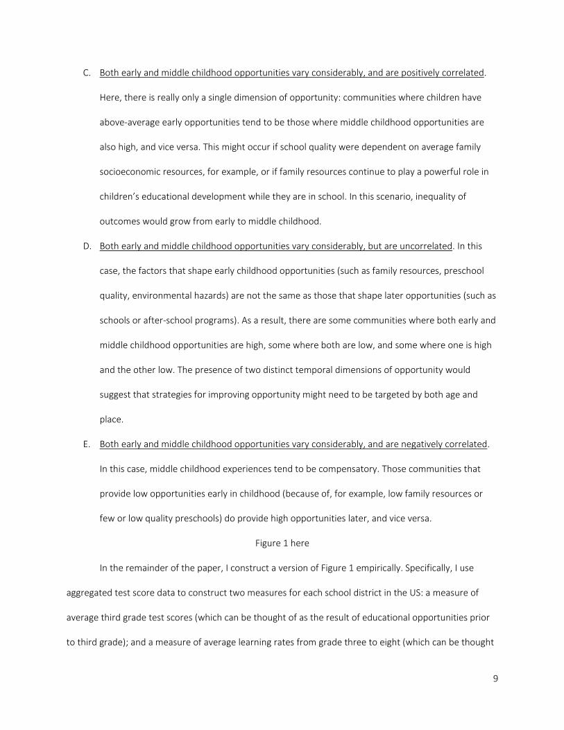
C. Both early and middle childhood opportunities vary considerably, and are positively correlated.

Here, there is really only a single dimension of opportunity: communities where children have

above-average early opportunities tend to be those where middle childhood opportunities are

also high, and vice versa. This might occur if school quality were dependent on average family

socioeconomic resources, for example, or if family resources continue to play a powerful role in

children’s educational development while they are in school. In this scenario, inequality of

outcomes would grow from early to middle childhood.

D. Both early and middle childhood opportunities vary considerably, but are uncorrelated. In this

case, the factors that shape early childhood opportunities (such as family resources, preschool

quality, environmental hazards) are not the same as those that shape later opportunities (such as

schools or after-school programs). As a result, there are some communities where both early and

middle childhood opportunities are high, some where both are low, and some where one is high

and the other low. The presence of two distinct temporal dimensions of opportunity would

suggest that strategies for improving opportunity might need to be targeted by both age and

place.

E. Both early and middle childhood opportunities vary considerably, and are negatively correlated.

In this case, middle childhood experiences tend to be compensatory. Those communities that

provide low opportunities early in childhood (because of, for example, low family resources or

few or low quality preschools) do provide high opportunities later, and vice versa.

Figure 1 here

In the remainder of the paper, I construct a version of Figure 1 empirically. Specifically, I use

aggregated test score data to construct two measures for each school district in the US: a measure of

average third grade test scores (which can be thought of as the result of educational opportunities prior

to third grade); and a measure of average learning rates from grade three to eight (which can be thought

10

of as the result of educational opportunities during late elementary and middle school). The underlying

data represent some 300 million standardized tests taken in grades 3-8 by roughly 45 million unique

students from 2009 to 2015. I use these data to construct measures of 1) average initial (third grade) test

scores and 2) growth rates of average scores in each district. Essentially, I partition each district’s average

eighth grade scores into two components—initial third grade levels and growth from third-eighth grade.

This partition provides information about the temporal structure of educational opportunity in each

school district.

Data

The test score data i use come from the Stanford Education Data Archive (SEDA), which includes

estimates of the average test scores—by school district, grade, year, subject, and race/ethnicity—of

students in almost every public school district in the United States (seda.stanford.edu). These estimates

are based on roughly 300 million state accountability test scores (taken by roughly 45 million students) on

math and English Language Arts (ELA) tests in grades 3-8 in the years 2009-2015 in every public school

district in the United States. Cells with fewer than 20 students are suppressed in public SEDA data.

The raw test score data used to construct the SEDA data come from the federal EDFacts data

collection system, which were provided by the National Center for Education Statistics under a restricted

data use license. The data include, for each public school in the United States, counts of students scoring

in each of several academic proficiency levels (often labeled something like “Below Basic,” “Basic,”

“Proficient,” and “Advanced”). These counts are disaggregated by race/ethnicity, grade (grades 3-8), test

subject (math and ELA), and year (school years 2008-09 through 2012-15).

In the SEDA data, school-level proficiency counts are used to estimate average scores in each

school district. Charter schools’ test scores are included in the public school district in which they are

formally chartered or, if not chartered by a district, in the district in which they are physically located.

11

Thus, in this paper I conceptualize a “school district” as a geographic catchment area that includes

students in all local charter schools as well as in traditional public schools. Virtual schools—online schools

that do not enroll students from any well-defined geographic area—are dropped from the sample. Such

schools enroll less than half of one percent of all students in the US.

The test scores in each state, grade, year, and subject are placed on a common scale, so that

performance can be meaningfully compared across states, grades, and years. First, each state’s test

scores are linked to the math and reading scales of the National Assessment of Education Progress

(NAEP). The NAEP scale is stable over time and is vertically linked from fourth to eighth grade; this allows

comparison of test scores among districts in different states and within a district across grades or years.

Second, the NAEP scale is transformed linearly to facilitate grade-level interpretations. In this new scale,

the national average 4th grade NAEP score in 2009 is anchored at 4; the national average 8th grade NAEP

score in 2013 is anchored at 8. A one unit different in scores is interpretable as the national average

difference between students one grade level apart (for much more detail on the linking method and

scale, see Reardon, Kalogrides and Ho 2017). Details on the source and construction of the estimates is

available on the SEDA website.

Any description of test score growth or change is dependent on the test metric used. The NAEP

scale (or the linear transformation of it we use) is useful because it was developed to allow comparisons

over time, across states, and across grades. Nonetheless, it is not the only defensible scaling of test

scores. Another potential metric is one in which test scores are standardized relative to the national

student test score distribution within each grade. In this scale, the average test score in each grade is 0

and the standard deviation is fixed at 1 in each grade. This is useful for comparing the relative magnitude

of differences in test scores in one grade to another grade, but it may distort information about relative

growth rates. If the variation in true skills grows over time, the standardized metric will necessarily

compress that growth and bias it toward zero, inducing a negative correlation between initial status and

12

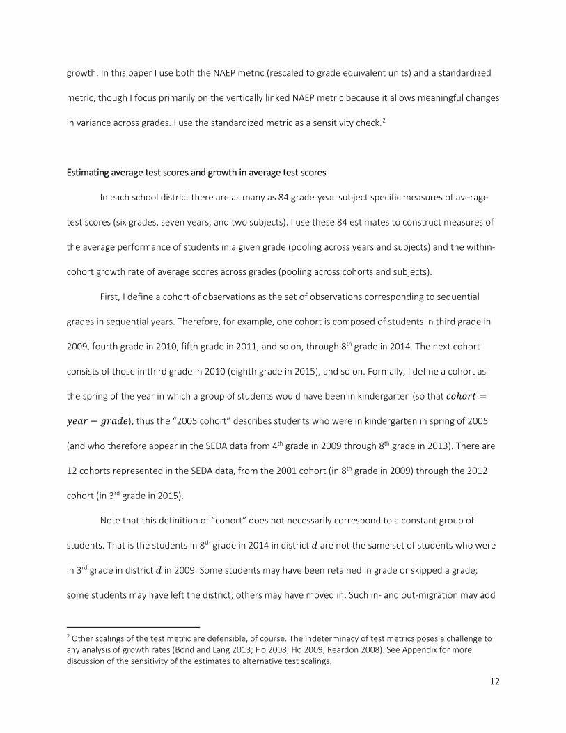
growth. In this paper I use both the NAEP metric (rescaled to grade equivalent units) and a standardized

metric, though I focus primarily on the vertically linked NAEP metric because it allows meaningful changes

in variance across grades. I use the standardized metric as a sensitivity check.2

Estimating average test scores and growth in average test scores

In each school district there are as many as 84 grade-year-subject specific measures of average

test scores (six grades, seven years, and two subjects). I use these 84 estimates to construct measures of

the average performance of students in a given grade (pooling across years and subjects) and the within-

cohort growth rate of average scores across grades (pooling across cohorts and subjects).

First, I define a cohort of observations as the set of observations corresponding to sequential

grades in sequential years. Therefore, for example, one cohort is composed of students in third grade in

2009, fourth grade in 2010, fifth grade in 2011, and so on, through 8th grade in 2014. The next cohort

consists of those in third grade in 2010 (eighth grade in 2015), and so on. Formally, I define a cohort as

the spring of the year in which a group of students would have been in kindergarten (so that 𝑐𝑐𝑐𝑐ℎ𝑐𝑐𝑜𝑜𝑜𝑜 =

𝑦𝑦𝑦𝑦𝑦𝑦𝑜𝑜 − 𝑔𝑔𝑜𝑜𝑦𝑦𝑔𝑔𝑦𝑦); thus the “2005 cohort” describes students who were in kindergarten in spring of 2005

(and who therefore appear in the SEDA data from 4th grade in 2009 through 8th grade in 2013). There are

12 cohorts represented in the SEDA data, from the 2001 cohort (in 8th grade in 2009) through the 2012

cohort (in 3rd grade in 2015).

Note that this definition of “cohort” does not necessarily correspond to a constant group of

students. That is the students in 8th grade in 2014 in district 𝑔𝑔 are not the same set of students who were

in 3rd grade in district 𝑔𝑔 in 2009. Some students may have been retained in grade or skipped a grade;

some students may have left the district; others may have moved in. Such in- and out-migration may add

2 Other scalings of the test metric are defensible, of course. The indeterminacy of test metrics poses a challenge to any analysis of growth rates (Bond and Lang 2013; Ho 2008; Ho 2009; Reardon 2008). See Appendix for more discussion of the sensitivity of the estimates to alternative test scalings.

13

random or systematic noise to our estimates of average growth rates; we may underestimate growth in

places where those who leave are disproportionately higher-achieving than those who move in.

Conversely, we may overestimate growth in places with the opposite in- and out-migration patterns or

with high retention rates. I discuss this more below.

Let �̂�𝜇𝑑𝑑𝑑𝑑𝑔𝑔𝑏𝑏 and 𝜔𝜔𝑑𝑑𝑑𝑑𝑔𝑔𝑏𝑏 = 𝑠𝑠𝑦𝑦��̂�𝜇𝑑𝑑𝑑𝑑𝑔𝑔𝑏𝑏� indicate the estimated average test score and its standard

error for students in district 𝑔𝑔 in year 𝑦𝑦, grade 𝑔𝑔, and subject 𝑏𝑏. Let 𝑔𝑔𝑜𝑜𝑔𝑔 ∈ (3,4,5,6,7,8) and 𝑐𝑐𝑐𝑐ℎ ∈

(2001, … ,2012) be continuous measures of grade and cohort, and let 𝑚𝑚𝑦𝑦𝑜𝑜ℎ ∈ (0,1) be a binary

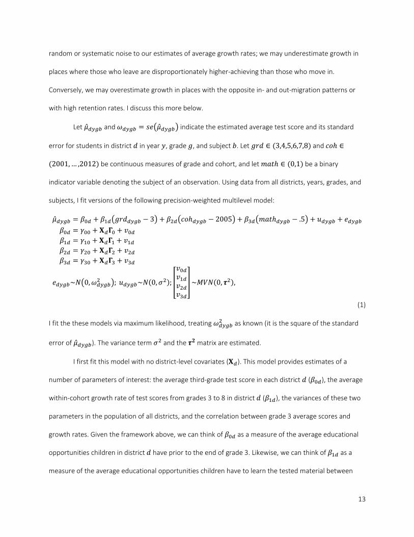
indicator variable denoting the subject of an observation. Using data from all districts, years, grades, and

subjects, I fit versions of the following precision-weighted multilevel model:

�̂�𝜇𝑑𝑑𝑑𝑑𝑔𝑔𝑏𝑏 = 𝛽𝛽0𝑑𝑑 + 𝛽𝛽1𝑑𝑑�𝑔𝑔𝑜𝑜𝑔𝑔𝑑𝑑𝑑𝑑𝑔𝑔𝑏𝑏 − 3� + 𝛽𝛽2𝑑𝑑�𝑐𝑐𝑐𝑐ℎ𝑑𝑑𝑑𝑑𝑔𝑔𝑏𝑏 − 2005�+ 𝛽𝛽3𝑑𝑑�𝑚𝑚𝑦𝑦𝑜𝑜ℎ𝑑𝑑𝑑𝑑𝑔𝑔𝑏𝑏 − .5� + 𝑢𝑢𝑑𝑑𝑑𝑑𝑔𝑔𝑏𝑏 + 𝑦𝑦𝑑𝑑𝑑𝑑𝑔𝑔𝑏𝑏 𝛽𝛽0𝑑𝑑 = 𝛾𝛾00 + 𝐗𝐗𝑑𝑑𝚪𝚪0 + 𝑣𝑣0𝑑𝑑 𝛽𝛽1𝑑𝑑 = 𝛾𝛾10 + 𝐗𝐗𝑑𝑑𝚪𝚪1 + 𝑣𝑣1𝑑𝑑 𝛽𝛽2𝑑𝑑 = 𝛾𝛾20 + 𝐗𝐗𝑑𝑑𝚪𝚪2 + 𝑣𝑣2𝑑𝑑 𝛽𝛽3𝑑𝑑 = 𝛾𝛾30 + 𝐗𝐗𝑑𝑑𝚪𝚪3 + 𝑣𝑣3𝑑𝑑

𝑦𝑦𝑑𝑑𝑑𝑑𝑔𝑔𝑏𝑏~𝑁𝑁�0,𝜔𝜔𝑑𝑑𝑑𝑑𝑔𝑔𝑏𝑏2 �; 𝑢𝑢𝑑𝑑𝑑𝑑𝑔𝑔𝑏𝑏~𝑁𝑁(0,𝜎𝜎2); �

𝑣𝑣0𝑑𝑑𝑣𝑣1𝑑𝑑𝑣𝑣2𝑑𝑑𝑣𝑣3𝑑𝑑

�~𝑀𝑀𝑀𝑀𝑁𝑁(0, 𝝉𝝉2),

(1)

I fit the these models via maximum likelihood, treating 𝜔𝜔𝑑𝑑𝑑𝑑𝑔𝑔𝑏𝑏2 as known (it is the square of the standard

error of �̂�𝜇𝑑𝑑𝑑𝑑𝑔𝑔𝑏𝑏). The variance term 𝜎𝜎2 and the 𝝉𝝉𝟐𝟐 matrix are estimated.

I first fit this model with no district-level covariates (𝐗𝐗𝑑𝑑). This model provides estimates of a

number of parameters of interest: the average third-grade test score in each district 𝑔𝑔 (𝛽𝛽0𝑑𝑑), the average

within-cohort growth rate of test scores from grades 3 to 8 in district 𝑔𝑔 (𝛽𝛽1𝑑𝑑), the variances of these two

parameters in the population of all districts, and the correlation between grade 3 average scores and

growth rates. Given the framework above, we can think of 𝛽𝛽0𝑑𝑑 as a measure of the average educational

opportunities children in district 𝑔𝑔 have prior to the end of grade 3. Likewise, we can think of 𝛽𝛽1𝑑𝑑 as a

measure of the average educational opportunities children have to learn the tested material between

14

grades 3 and 8. The average test scores in district 𝑔𝑔 in 8th grade are therefore the sum of average grade 3

scores and 5 years of growth: 𝛽𝛽0𝑑𝑑 + 5𝛽𝛽1𝑑𝑑.

Because �̂�𝜇𝑑𝑑𝑑𝑑𝑔𝑔𝑏𝑏 is scaled to have an average value of 4 among 4th graders in 2009 and an average

of 8 among 8th graders in 2013, the coefficients 𝛽𝛽0𝑑𝑑 and 𝛽𝛽1𝑑𝑑 reflect grade-levels units. Note that 𝛽𝛽0𝑑𝑑 = 3

implies that students in district 𝑔𝑔 have the same average scores in 3rd grade as the average 2008 third

grader in the US. Likewise, 𝛽𝛽1𝑑𝑑 = 1 implies that students in district 𝑔𝑔 have the same average learning rate

from grade 3 to 8 as the average student in the US (in the 2005 cohort). A value of 𝛽𝛽1𝑑𝑑 = 1.1 or 𝛽𝛽1𝑑𝑑 =

0.90, for example, would imply that the performance of the average student in district 𝑔𝑔 improves or

declines, respectively, 10 percent (one-tenth of a grade-level per year) faster or slower, respectively, than

the average public school student in the US from 3rd to 8th grade.

Of particular interest here is the joint distribution of 𝛽𝛽0𝑑𝑑 and 𝛽𝛽1𝑑𝑑. This is given by ��𝛾𝛾00𝛾𝛾10� , 𝝉𝝉[01]

2 �,

where 𝝉𝝉[01]2 = �

𝜏𝜏00 𝜏𝜏01𝜏𝜏01 𝜏𝜏11� is the 2-x-2 upper-left submatrix of 𝝉𝝉2. This joint distribution is our primary

focus: 𝜏𝜏00 and 𝜏𝜏11 describe the variances of 𝛽𝛽0𝑑𝑑 and 𝛽𝛽1𝑑𝑑, respectively, and their correlation is computed

as 𝑜𝑜01 = 𝜏𝜏01(𝜏𝜏00 ∙ 𝜏𝜏11)−1/2. Note that I estimate the covariance matrix 𝝉𝝉[01]2 via maximum likelihood

using the model above. I do not calculate the variances and covariances based on the estimated (and

therefore error-prone) 𝛽𝛽0𝑑𝑑’s and 𝛽𝛽1𝑑𝑑’s.

In addition to providing estimates of the parameters of the joint distribution of 𝛽𝛽0𝑑𝑑 and 𝛽𝛽1𝑑𝑑, the

model also provides estimates of 𝛽𝛽0𝑑𝑑 and 𝛽𝛽1𝑑𝑑 for each district. I use the Empirical Bayes (EB) “shrunken”

estimates of these parameters, denoted 𝛽𝛽0𝑑𝑑∗ and 𝛽𝛽1𝑑𝑑∗ . The model provides estimates of the reliability of

each of these estimates; as well as a measure of their average reliability.

The other coefficients in the model are of less direct interest for our purposes here. 𝛽𝛽2𝑑𝑑 indicates

the average within-grade (cohort-to-cohort) change per year in average test scores in district 𝑔𝑔; and 𝛽𝛽3𝑑𝑑

indicates the average (within grade and year) difference in math and reading scores in district 𝑔𝑔.

15

To estimate the association between district characteristics (denoted by the vector 𝐗𝐗𝑑𝑑) and

average test scores (𝛽𝛽0𝑑𝑑) and test score growth (𝛽𝛽1𝑑𝑑), I fit models that add 𝐗𝐗𝑑𝑑 as predictors of the district

parameters in Model (1) above.

Measuring average socioeconomic status among students enrolled in a school district

In order to measure the socioeconomic characteristics of the families of children, I use data from

the American Community Survey (ACS). The ACS includes detailed socio-demographic data for families

living in each school district in the U.S.; these tabulations are available through the School District

Demographic System (SDDS). I use data from the 2006-10 SDDS tabulations because they include

tabulations of family characteristics among families with school-age children enrolled in public schools.

In particular, I use six measures of the socioeconomic composition of families living in a district

with children enrolled in public schools: 1) median family income; 2) percent of adults with a bachelor’s

degree or higher degree; 3) poverty rate; 4) unemployment rate; 5) Supplemental Nutritional Assistance

Program (SNAP) eligibility rate; and 6) the percent of families headed by a single mother. Each of these is

available separately by race/ethnicity (for racial/ethnic groups of sufficient local population size).

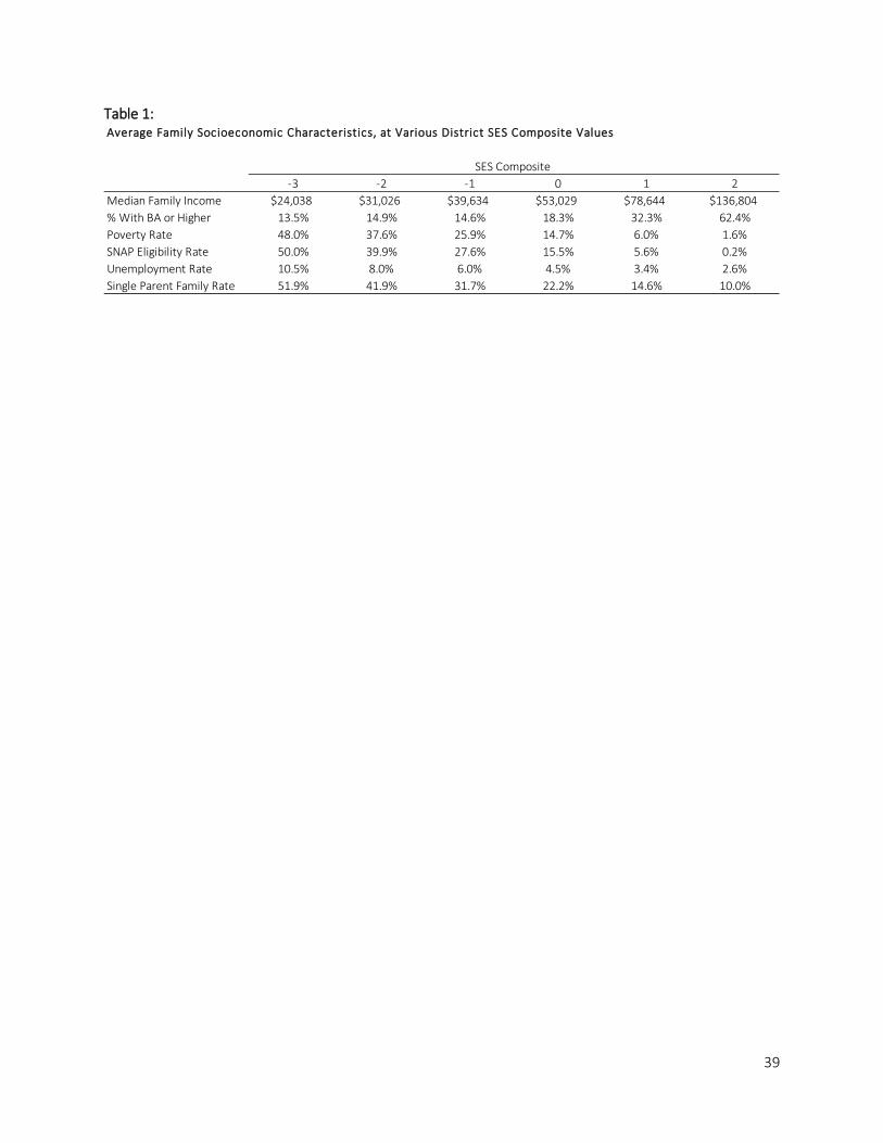
I construct a measure of each district’s average socioeconomic status as the first principal

component of the six measures above. This measure is standardized to have a mean of zero and a

standard deviation of 1. To give a sense of how this measure is scaled, Table 1 describes the average

characteristics of school districts at various values of the SES composite.

Table 1 here

Analytic sample

The data I use here include 11,315 school districts for which I am able to compute a

socioeconomic status variable and for which the SEDA data include measures of academic achievement.

16

Districts not included in the sample are predominantly very small districts for which samples are too small

for SDDS to report socioeconomic characteristics or that have fewer than 20 students total per grade (in

which case the SEDA data do not include estimates of average test scores). There are 824 districts for

which the ACS SES variable cannot be constructed; these are small districts (averaging 43 students per

grade) and contain fewer than 1% of US public school students. The 11,315 districts in the analytic sample

collectively enroll roughly 3.7 million students per grade (roughly 99% of all public school students in the

U.S.).

How do grade three average scores and growth rates vary among districts?

Model 1 provides estimates of the average grade 3 test scores and the average grade 3-8 growth

rate in each district. Importantly, it also provides maximum likelihood estimates of the variances and

correlation of these parameters; the maximum likelihood estimates are not biased by noise in each

district’s estimated parameters. Recall that we can think of the grade three test score average as a

measure of “early educational opportunities” in a district; the growth rate serves as a proxy for “growth

opportunities”—the extent of educational opportunities in grades three to eight.

Table 2 presents the parameters describing the joint distribution these two measures. The left

panel reports the results based on the preferred grade-equivalent NAEP scale; the right panel reports

comparable results based on the standardized scale. Each panel includes a column for math and ELA

scores, as a well as results from the model that pools the data and estimates a common grade 3 level and

growth rate for both subjects.

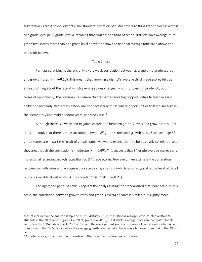
In the average school district, 3rd grade average test scores are roughly one-sixth of a grade level

above the national average, and increase by 0.97 grade levels per grade.3 By third grade, test scores vary

3 Note that there are three reasons that the average district’s scores are not equal to the national average. First, more small districts have above average test scores and slightly lower than average growth rates, so the unweighted averages across districts are not identical to the enrollment-weighted averages. Second, some very small districts

17

substantially across school districts. The standard deviation of district average third grade scores is almost

one grade level (0.98 grade levels), meaning that roughly one third of school districts have average third

grade test scores more than one grade level above or below the national average (one sixth above and

one sixth below).

Table 2 here

Perhaps surprisingly, there is only a very weak correlation between average third grade scores

and growth rates (𝑜𝑜 = −0.13). This means that knowing a district’s average third grade scores tells us

almost nothing about the rate at which average scores change from third to eighth grade. Or, put in

terms of opportunity, the communities where children experience high opportunities to learn in early

childhood and early elementary school are not necessarily those where opportunities to learn are high in

the elementary and middle school years, and vice versa.4

Although there is a weak and negative correlation between grade 3 levels and growth rates, that

does not imply that there is no association between 8th grade scores and growth rates. Since average 8th

grade scores are in part the result of growth rates, we would expect them to be positively correlated, and

they are, though the correlation is moderate (𝑜𝑜 = 0.49). This suggests that 8th grade average scores carry

more signal regarding growth rates than do 3rd grade scores. However, if we estimate the correlation

between growth rates and average scores across all grades 3-8 (which is more typical of the level of detail

publicly available about schools), the correlation is small (𝑜𝑜 = 0.21).

The righthand panel of Table 2 repeats the analysis using the standardized test score scale. In this

scale, the correlation between growth rates and grade 3 average scores is similar, but slightly more

are not included in the analytic sample of 11,315 districts. Third, the national average is constructed relative to students in the 2009 cohort (grade 4 in 2009, grade 8 in 2013), but districts’ average scores are computed for all cohorts in the SEDA data (cohorts 2001-2012) and the average third grade scores over all cohorts were a bit higher than those in the 2005 cohort, while the average growth rate over all cohorts was a bit lower than that of the 2005 cohort. 4 As noted above, this correlation is sensitive to the scale used to measure test scores.

18

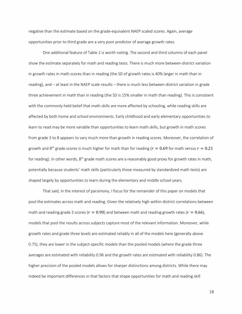
negative than the estimate based on the grade-equivalent NAEP scaled scores. Again, average

opportunities prior to third grade are a very poor predictor of average growth rates.

One additional feature of Table 2 is worth noting. The second and third columns of each panel

show the estimate separately for math and reading tests. There is much more between-district variation

in growth rates in math scores than in reading (the SD of growth rates is 40% larger in math than in

reading), and – at least in the NAEP scale results – there is much less between-district variation in grade

three achievement in math than in reading (the SD is 15% smaller in math than reading). This is consistent

with the commonly-held belief that math skills are more affected by schooling, while reading skills are

affected by both home and school environments. Early childhood and early elementary opportunities to

learn to read may be more variable than opportunities to learn math skills, but growth in math scores

from grade 3 to 8 appears to vary much more than growth in reading scores. Moreover, the correlation of

growth and 8th grade scores is much higher for math than for reading (𝑜𝑜 = 0.69 for math versus 𝑜𝑜 = 0.21

for reading). In other words, 8th grade math scores are a reasonably good proxy for growth rates in math,

potentially because students’ math skills (particularly those measured by standardized math tests) are

shaped largely by opportunities to learn during the elementary and middle school years.

That said, in the interest of parsimony, I focus for the remainder of this paper on models that

pool the estimates across math and reading. Given the relatively high within-district correlations between

math and reading grade 3 scores (𝑜𝑜 = 0.90) and between math and reading growth rates (𝑜𝑜 = 0.66),

models that pool the results across subjects capture most of the relevant information. Moreover, while

growth rates and grade three levels are estimated reliably in all of the models here (generally above

0.75), they are lower in the subject-specific models than the pooled models (where the grade three

averages are estimated with reliability 0.96 and the growth rates are estimated with reliability 0.86). The

higher precision of the pooled models allows for sharper distinctions among districts. While there may

indeed be important differences in that factors that shape opportunities for math and reading skill

19

development, those issues are outside the scope of my analysis here.

How large is the variation in growth rates?

It is clear from Table 2 that average test scores in grade 3 are uninformative as predictors of

growth rates, perhaps that is because there is relatively little variation in growth rates. It is useful

therefore to quantify the magnitude of the variation in growth rates. The standard deviation of growth

rates is 0.135 grade levels/year, or equivalently, 0.675 grade levels from grade 3 to 8. This means that in

roughly one-sixth of districts test scores improve by two-thirds or more of a grade level from grades 3 to

8; in another one-sixth of districts scores fall behind by two-thirds or more of a grade level. Another way

to quantify this is to note that a growth rate of 1.135 indicates that students’ scores increase 13.5% faster

than the national average (a note that increase of 13.5% of a school year is roughly an additional 25

school days/year in the typical district, not a trivial amount). So there is considerable variation among

school districts in average growth rates.

Another way to quantify the relative magnitude of the variation in district test score growth rates

is to compare the magnitude of between-district variation in growth rates to the magnitude of between-

district variation in grade 3 test scores. Consider two school districts, one in which students’ third grade

scores are at the national average but growth rates are one standard deviation above the national

average; and one in which students’ third grade scores are one standard deviation above the national

average but growth rates are at the national average. In which district are students’ scores higher by

eighth grade, and by how much? These calculations are shown in the bottom panel of Table 2.

A standard deviation difference in growth rates experienced over 5 years from grade 3 to 8 is

equivalent to a 70% of a district standard deviation in grade three levels. That is, in 5 years, students in

the average-early-opportunity/high-growth-opportunity district make up 70% of the grade three gap

relative to a high-early-opportunity/average-growth-opportunity district. These results hold in both the

20

reported scales.

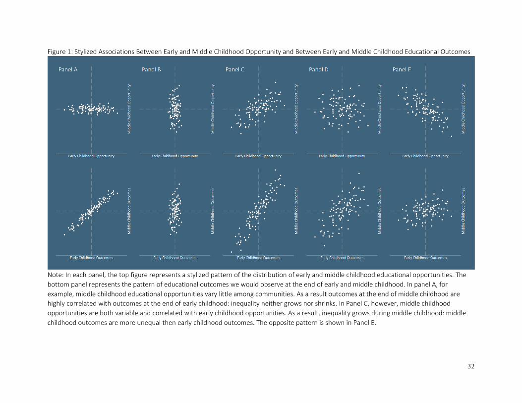
Where in the US are growth opportunities highest?

Figures 2 and 3 display the geographic patterns of grade 3 average scores and grade 3-8 growth

rates. Figure 2 shows that opportunities prior to grade 3 are highest in many of suburban and exurban

school districts around metropolitan areas, particularly in the northeast, Midwest, and the California

coast, and are low in much of the Deep South and the rural West. Growth opportunities in contrast are

more varied. Tennessee is characterized by moderately low third grade scores but above average growth

rates; Florida, in contrast, is characterized by slightly above average scores in grade 3 but very low

average growth.

Figures 2 and 3 here

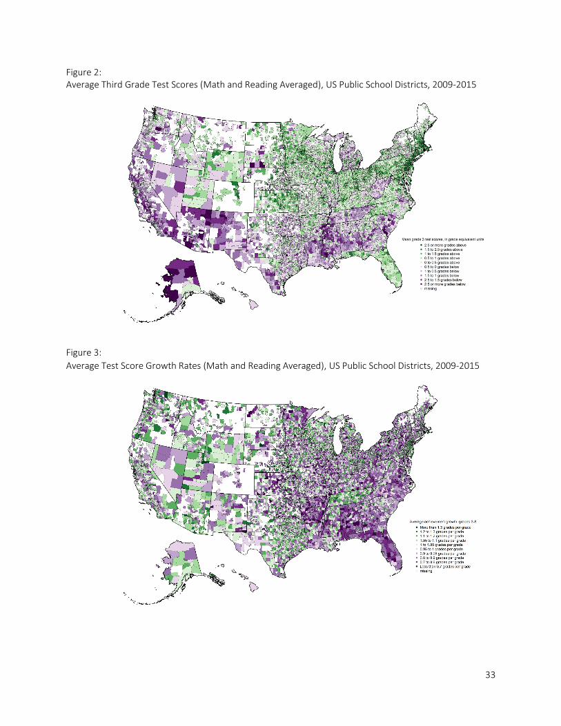
Both Table 2 and Figures 2 and 3 indicate both that there is considerable variation in both grade 3

average scores and growth rates, but that they are not highly correlated. This is more explicitly evident in

Figure 4, which plots each district’s estimated growth rate (on the vertical axis) against its grade 3-8

growth rate. The plot uses the EB estimates �̂�𝛽0𝑑𝑑∗ and �̂�𝛽1𝑑𝑑∗ ; imprecisely estimated values are shrunken

toward the overall mean. Note that district estimates with a reliability less than 0.7 are not included in

this or other figures (though their data are included in fitting Model 1).

Figure 4 here

Figure 4 makes clear that there is very little relationship between average third grade test scores

and average growth. The figure can be divided into 4 quadrants defined by districts’ early educational

opportunity and growth opportunities. In the upper right are districts characterized by high early

educational opportunity and high growth opportunity; these are districts where students have high

average achievement in grade 3 and have above average growth rates following that. In the lower left are

districts characterized by the opposite pattern: low early and low-growth opportunity. The off-diagonal

21

quadrants have high early/low growth and low early/high growth opportunity structures, respectively.

The striking feature of Figure 4 is the absence of a correlation between growth and initial scores.

Among districts with high grade 3 scores there are many with high growth and many with low growth; the

same is true among those with low initial scores. This suggests there is no significant floor or ceiling effect

in the estimates (which is not surprising given that the data points reflect district average scores not

individual student scores). Even among school districts with very high scores in third grade (three grade

levels above average), some districts have very high growth; the same is true among initially low-

performing districts.

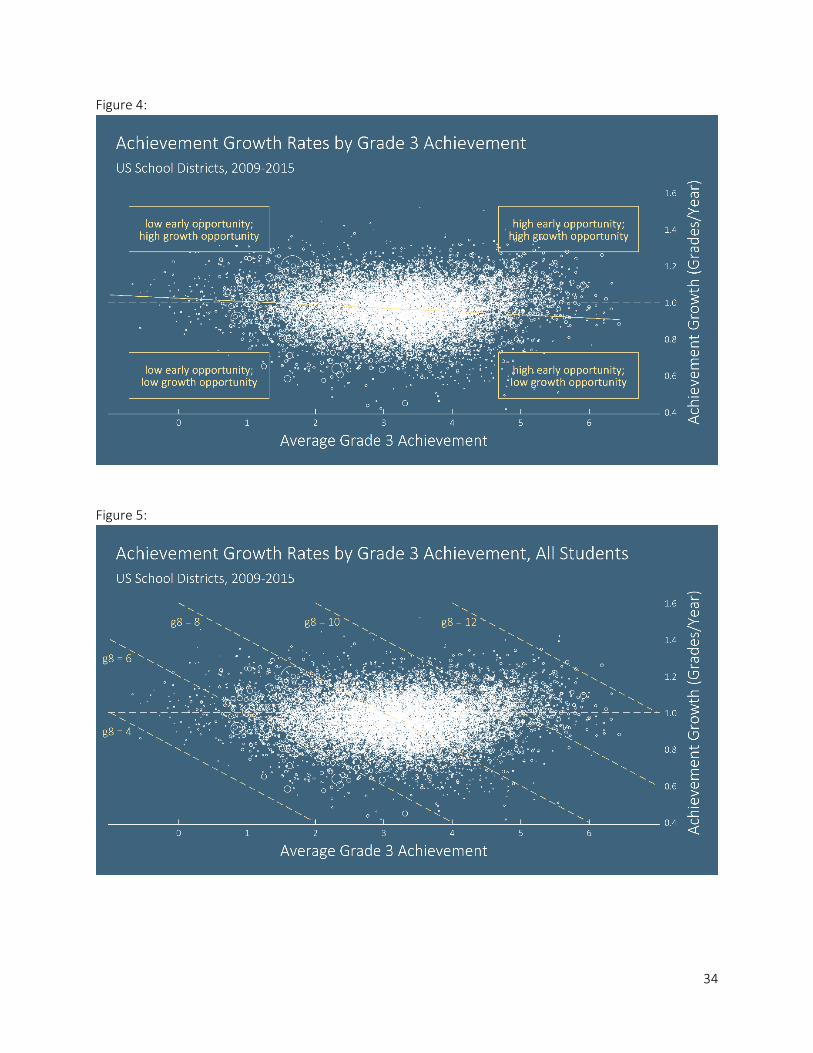
Another perspective on Figure 4 is provided by considering districts with the same 8th grade

average scores. The lack of a substantial correlation between growth and grade 3 scores implies that,

among districts with the same 8th average grade scores, some have higher grade 3 scores and lower

growth while others have lower initial status and higher growth. Figure 5 illustrates this: the plot is the

same as Figure 4, but with lines representing levels of grade 8 average achievement drawn as isobars on

the plot. Districts that fall anywhere on an isobar have the same average 8th grade achievement, despite

differences in initial status and growth rates. For example, a district where initial scores are one grade

level below and the average growth rates is 1.2 will have the same average 8th grade scores as one where

initial scores are one grade level above average but growth rates are 0.8 (both districts will fall on the

g8=8 line).

Figure 5 here

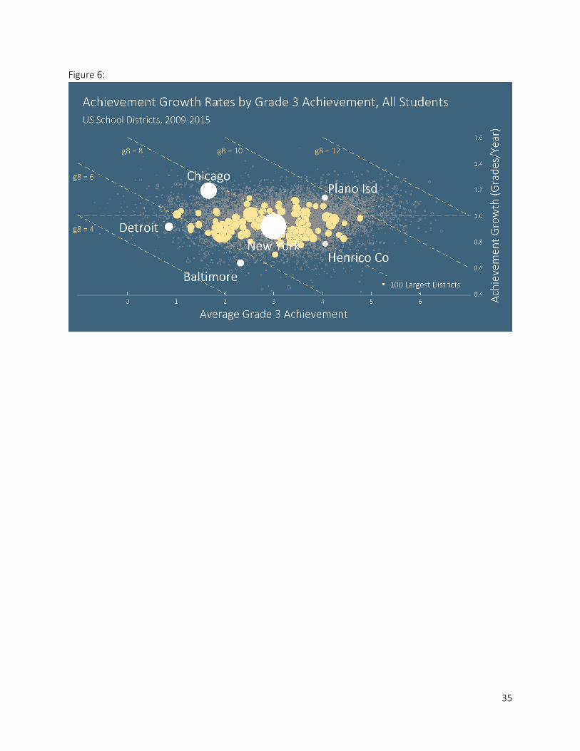
Chicago, for example (see Figure 6), has average 3rd grade test scores well below the national

average (about 1.4 grade levels below), but very high growth rates. New York City students have both

average third grade scores and average growth rates. And in Henrico County, VA (suburban Richmond),

third grade test scores are very high but growth rates are very low. As a result, 8th grade scores in

Chicago, New York, and Henrico County are very similar (within a half grade level of each other) despite a

22

range of 2.5 grade levels difference in their 3rd grade scores. Likewise, Detroit and Baltimore 8th grade test

scores are very similar to one another (and very low, over 2.5 grade levels below the national average),

but in Baltimore the low 8th grade scores are more the result of very low growth opportunities than low

early opportunities, the opposite of Detroit.

Figure 6 here

Figure 6 highlights the 100 largest school districts in the U.S. The substantial variation among

them on both the early and growth opportunity dimensions suggests that the variation evident in Figures

3-5 is not simply the result of idiosyncratic variation among small school districts or sampling noise. Each

of these districts’ estimates are based on hundreds of thousands or millions of test scores (Chicago’s

estimate is based on over 2 million test scores, for example).

How is average test score growth related to district socioeconomic status?

Figure 7 displays the association between the socioeconomic status measure and both grade 3

average scores (upper figure) and growth rates (lower figure). The fitted lines are estimated from a

version of Model 1 that includes a cubic function of socioeconomic status (SES) as a predictor of each of

the four distrct-level parameters in the model. SES is positively associated with grade three scores and

growth rates, but the association is much stronger with grade 3 average scores (𝑜𝑜 = 0.68) than with

growth rates (𝑜𝑜 = .32). These associations are shown graphically in Figure 7.

Figure 7 here

It may seem strange that both grade 3 average scores and growth rates are higher, on average, in

high-SES districts than in low-SES districts, but grade 3 average scores and growth are slightly negatively

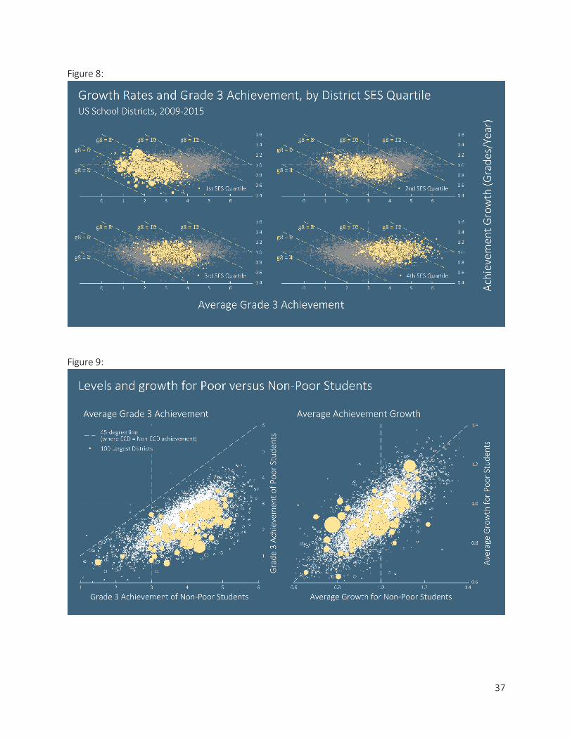
correlated. Figure 8 helps to clarify the patterns these patterns. Each panel of the figure highlights

districts in a given SES quartile. Low-SES districts have generally, but not always, low average third grade

scores, and many have lower than average growth rates. High-SES districts, in contrast, generally have

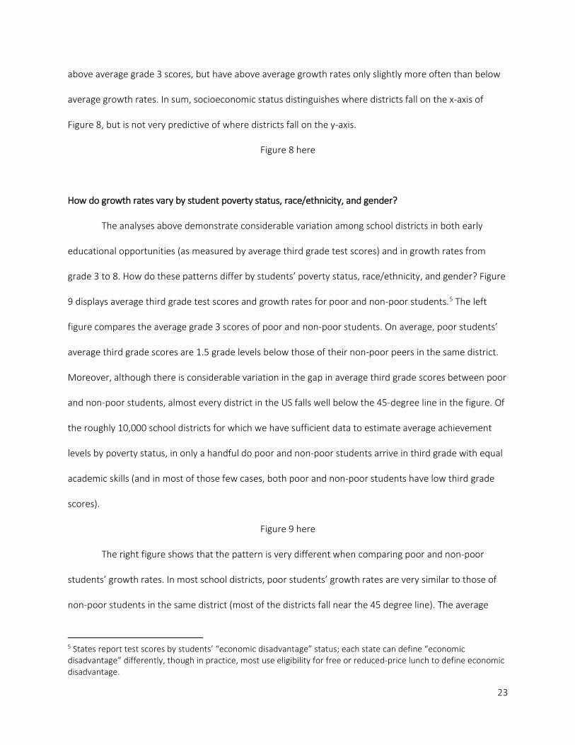
23

above average grade 3 scores, but have above average growth rates only slightly more often than below

average growth rates. In sum, socioeconomic status distinguishes where districts fall on the x-axis of

Figure 8, but is not very predictive of where districts fall on the y-axis.

Figure 8 here

How do growth rates vary by student poverty status, race/ethnicity, and gender?

The analyses above demonstrate considerable variation among school districts in both early

educational opportunities (as measured by average third grade test scores) and in growth rates from

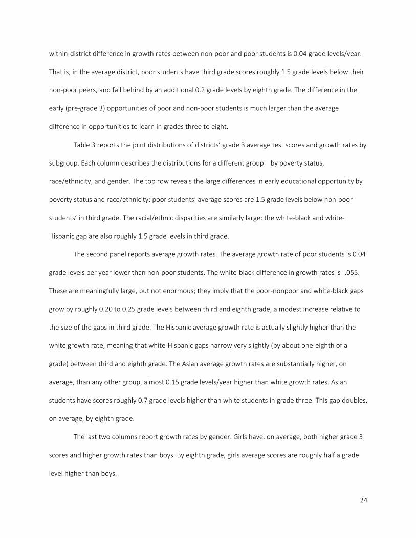
grade 3 to 8. How do these patterns differ by students’ poverty status, race/ethnicity, and gender? Figure

9 displays average third grade test scores and growth rates for poor and non-poor students.5 The left

figure compares the average grade 3 scores of poor and non-poor students. On average, poor students’

average third grade scores are 1.5 grade levels below those of their non-poor peers in the same district.

Moreover, although there is considerable variation in the gap in average third grade scores between poor

and non-poor students, almost every district in the US falls well below the 45-degree line in the figure. Of

the roughly 10,000 school districts for which we have sufficient data to estimate average achievement

levels by poverty status, in only a handful do poor and non-poor students arrive in third grade with equal

academic skills (and in most of those few cases, both poor and non-poor students have low third grade

scores).

Figure 9 here

The right figure shows that the pattern is very different when comparing poor and non-poor

students’ growth rates. In most school districts, poor students’ growth rates are very similar to those of

non-poor students in the same district (most of the districts fall near the 45 degree line). The average

5 States report test scores by students’ “economic disadvantage” status; each state can define “economic disadvantage” differently, though in practice, most use eligibility for free or reduced-price lunch to define economic disadvantage.

24

within-district difference in growth rates between non-poor and poor students is 0.04 grade levels/year.

That is, in the average district, poor students have third grade scores roughly 1.5 grade levels below their

non-poor peers, and fall behind by an additional 0.2 grade levels by eighth grade. The difference in the

early (pre-grade 3) opportunities of poor and non-poor students is much larger than the average

difference in opportunities to learn in grades three to eight.

Table 3 reports the joint distributions of districts’ grade 3 average test scores and growth rates by

subgroup. Each column describes the distributions for a different group—by poverty status,

race/ethnicity, and gender. The top row reveals the large differences in early educational opportunity by

poverty status and race/ethnicity: poor students’ average scores are 1.5 grade levels below non-poor

students’ in third grade. The racial/ethnic disparities are similarly large: the white-black and white-

Hispanic gap are also roughly 1.5 grade levels in third grade.

The second panel reports average growth rates. The average growth rate of poor students is 0.04

grade levels per year lower than non-poor students. The white-black difference in growth rates is -.055.

These are meaningfully large, but not enormous; they imply that the poor-nonpoor and white-black gaps

grow by roughly 0.20 to 0.25 grade levels between third and eighth grade, a modest increase relative to

the size of the gaps in third grade. The Hispanic average growth rate is actually slightly higher than the

white growth rate, meaning that white-Hispanic gaps narrow very slightly (by about one-eighth of a

grade) between third and eighth grade. The Asian average growth rates are substantially higher, on

average, than any other group, almost 0.15 grade levels/year higher than white growth rates. Asian

students have scores roughly 0.7 grade levels higher than white students in grade three. This gap doubles,

on average, by eighth grade.

The last two columns report growth rates by gender. Girls have, on average, both higher grade 3

scores and higher growth rates than boys. By eighth grade, girls average scores are roughly half a grade

level higher than boys.

25

Table 3 here

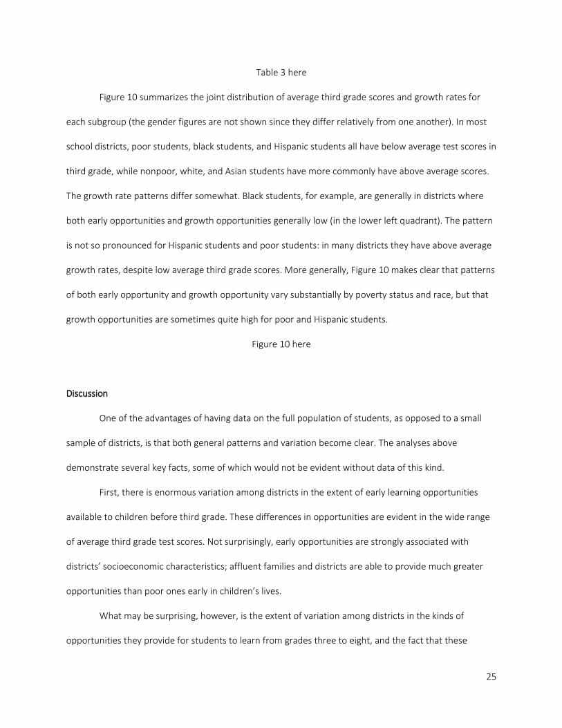
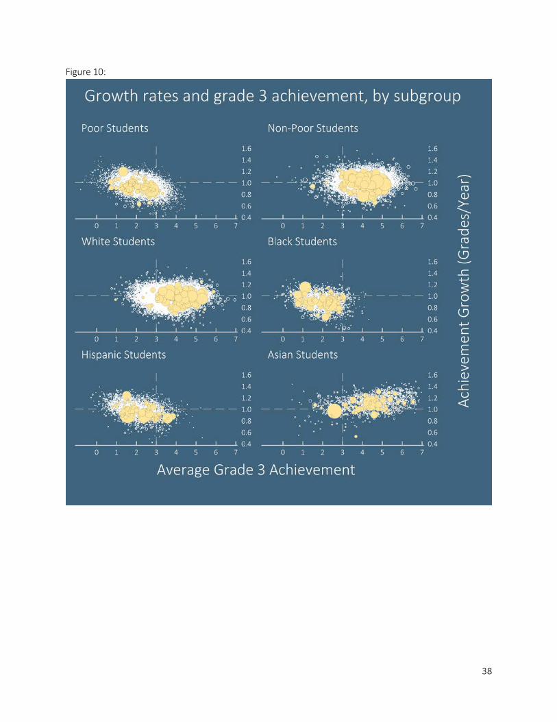
Figure 10 summarizes the joint distribution of average third grade scores and growth rates for

each subgroup (the gender figures are not shown since they differ relatively from one another). In most

school districts, poor students, black students, and Hispanic students all have below average test scores in

third grade, while nonpoor, white, and Asian students have more commonly have above average scores.

The growth rate patterns differ somewhat. Black students, for example, are generally in districts where

both early opportunities and growth opportunities generally low (in the lower left quadrant). The pattern

is not so pronounced for Hispanic students and poor students: in many districts they have above average

growth rates, despite low average third grade scores. More generally, Figure 10 makes clear that patterns

of both early opportunity and growth opportunity vary substantially by poverty status and race, but that

growth opportunities are sometimes quite high for poor and Hispanic students.

Figure 10 here

Discussion

One of the advantages of having data on the full population of students, as opposed to a small

sample of districts, is that both general patterns and variation become clear. The analyses above

demonstrate several key facts, some of which would not be evident without data of this kind.

First, there is enormous variation among districts in the extent of early learning opportunities

available to children before third grade. These differences in opportunities are evident in the wide range

of average third grade test scores. Not surprisingly, early opportunities are strongly associated with

districts’ socioeconomic characteristics; affluent families and districts are able to provide much greater

opportunities than poor ones early in children’s lives.

What may be surprising, however, is the extent of variation among districts in the kinds of

opportunities they provide for students to learn from grades three to eight, and the fact that these

26

growth opportunities are at best weakly correlated with early opportunities and with socioeconomic

status. The empirical patterns evident presented above are most similar to the scenario described in

Panel D of Figure 1 above: both early and middle childhood opportunities vary widely among school

districts, but do not covary significantly.

It is tempting to think of growth rates in test scores as a rough measure of school district

effectiveness. This is neither entirely inappropriate nor entirely accurate. The growth rates better isolate

the contribution to learning due to experiences during the schooling years. Grade 3 average scores are

likely much more strongly influenced by early childhood experiences than the growth rates. So the

growth rates are certainly better as measures of educational opportunities from age 9 to 14 than are

average test scores in a school district. But that does not mean they reflect only the contribution of

schooling. Other characteristics of communities, including family resources, after school programs, and

neighborhood conditions may all affect growth in test scores independent of schools’ effects. Some

caution is warranted in interpreting the average growth rates as pure measures of school effectiveness.

Nonetheless, relative to average test scores (at grade 3 or any grade), the growth rates are closer to a

measure of school effectiveness. Given that schooling plays a significant role in children’s lives from age 9

to 14 (at least in terms of time spent), it is not unreasonable to think that the growth measures carry

some signal regarding school quality—and more signal than contained in simple average test score

measures.

If we take the growth rates, then, as rough measures of school effectiveness, then neither

socioeconomic conditions nor average test scores are very informative about school district effectiveness.

Many districts with high average test scores have low growth rates, and vice versa. And many low-income

districts have above average growth rates. This finding calls into question the use of average test scores

as an accountability tool or a way of evaluating schools. Because average test scores, even in eighth

grade, are only weakly correlated with growth rates, any system that rewards or sanctions schools or

27

districts on the basis of their average scores will necessarily do so inappropriately in many cases

(assuming that we wish to incentivize growth rates). And any information system that makes average test

scores publicly available to parents in the hopes that a market for high test score districts will emerge and

drive school improvement may instead simply create a market for high-SES districts, increasing economic

segregation without improving school systems. To the extent that public information about school quality

affects middle- and high-income families’ decisions about where to live, information on growth rates

might provide very different signals, perhaps leading to lower levels of economic residential and school

segregation.

That is not to say the growth rates of the type I have calculated here–using repeated cross-

sectional aggregated data—are ideal, but they almost certainly are better signals of the learning

opportunities available in a school district than are average test scores. If we used measures like these as

one part of an accountability system or a public information system, schools in the upper-left quadrant

would be preferred (at least in grades 3-8) over districts in the lower-right quadrant. Future research

might compare the growth measures I construct here with growth measures based on longitudinal

student-level data. Such measures would be immune from the potential noise in my measures that arises

because of district in- and out-migration and/or grade retention.

The findings here also provide some insight into the issues raised in the opening of this paper. Are

schools engines of opportunity or agents of inequality? The answer is perhaps more nuanced than the

question implies. Some school districts seem to provide high opportunities for children from low-income

families during elementary and middle school; others do not. That suggests our school systems (or other

community institutions) have the potential to catalyze opportunity, but that potential is incompletely

realized in many places. And although poverty is systematically associated with low opportunities to learn

in early childhood, as evidenced by the consistently low average third grade test scores in low-income

districts, poverty very clearly does not strictly determine the opportunities for children to learn in the

28

middle grade years. That said, it is not clear from the patterns here that an effective school system alone

can make up for low opportunities in early childhood. The large gaps in students’ academic skills between

low- and higher-SES districts are so large that even the highest growth rate in the country would be

insufficient to close even half of the gap by eighth grade.

These patterns have implications both for education policy and for our understanding of the

potentially equalizing role of schools. In terms of policy, they suggest that levels of student outcomes are

a poor measure of school effectiveness. I am certainly not the first to say this, but the data from 11,000

school districts demonstrate the point very clearly. The findings also suggest that we could learn a great

deal about reducing educational inequality from the low-SES communities with high growth rates. They

provide, at a minimum, an existence proof of the possibility that even schools in high-poverty

communities can be effective. Now the challenge is to learn what conditions make that possible and how

we can foster the same conditions everywhere.

29

References Abdulkadiroglu, Atila, Joshua Angrist, Susan Dynarski, Thomas J. Kane, and Parag Pathak. 2011.

"Accountability and Flexibility in Public Schools: Evidence From Boston's Charters and Pilots." Quarterly Journal of Economics 126(2):699-748.

Alexander, Karl L., Doris R. Entwisle, and Linda S. Olson. 2001. "Schools, Achievement, and Inequality: A Seasonal Perspective." Educational Evaluation and Policy Analysis 23(2):171-91.

Alexander, Karl L., Doris R. Entwisle, and Linda Steffel Olson. 2007. "Lasting Consequences of the Summer Learning Gap." American Sociological Review 72(April):167-80.

Bloom, Howard S, Carolyn J Hill, Alison Rebeck Black, and Mark W Lipsey. 2008. "Performance trajectories and performance gaps as achievement effect-size benchmarks for educational interventions." Journal of Research on Educational Effectiveness 1(4):289-328.

Bloom, Howard S., and Rebecca Unterman. 2012. "Sustained Positive Effects on Graduation Rates Produced by New York City’s Small Public High Schools of Choice." New York: MDRC.

Bond, Timothy N., and Kevin Lang. 2013. "The Black-White Education-Scaled Test-Score Gap In Grades K-7." National Bureau of Economic Research Working Paper 19243.

Bowles, Samuel, and Herbert Gintis. 1976. Schooling in capitalist America: Educational reform and the contradictions of economic life. New York: Basic Books.

Boyd, Donald, Hamilton Lankford, Susanna Loeb, and James Wyckoff. 2005. "Explaining the short careers of high-achieving teachers in schools with low-performing students." The American Economic Review 95(2):166-71.

Center for Research on Education Outcomes (CREDO). 2015. "National Charter School Study." Stanford, CA: Stanford University.

Chetty, Raj, John N Friedman, Emmanuel Saez, Nicholas Turner, and Danny Yagan. 2017. "Mobility report cards: The role of colleges in intergenerational mobility." National Bureau of Economic Research.

Chetty, Raj, Nathaniel Hedren, Patrick Kline, and Emmanuel Saez. 2014. "Where is the land of opportunity? The geography of intergenerational mobility in the United States." National Bureau of Economic Research Working Paper 19843.

Chetty, Raj, Nathaniel Hendren, and Lawrence F Katz. 2016. "The effects of exposure to better neighborhoods on children: New evidence from the Moving to Opportunity experiment." The American Economic Review 106(4):855-902.

Chetty, Raj, Nathaniel Hendren, and Lawrence F. Katz. 2015. "The effects of exposure to better neighborhoods on children: New evidence from the Moving to Opportunity experiment." Harvard University.

Coleman, James S., Ernest Q. Campbell, Carol J. Hobson, James McPartland, Alexander M. Mood, Frederick D. Weinfeld, and Robert L. York. 1966. Equality of educational opportunity. Washington, DC: U.S. Department of Health, Education, and Welfare, Office of Education.

Dadey, Nathan, and Derek C Briggs. 2012. "A Meta-Analysis of Growth Trends from Vertically Scaled Assessments." Practical Assessment, Research & Evaluation 17.

Darling-Hammond, Linda. 1998. "Unequal opportunity: Race and education." The Brookings Review 16(2):28.

Dobbie, Will, Roland G Fryer, and G Fryer Jr. 2011. "Are high-quality schools enough to increase achievement among the poor? Evidence from the Harlem Children's Zone." American Economic Journal: Applied Economics 3(3):158-87.

Downey, Douglas B., and Dennis J. Condron. 2016. "Fifty Years since the Coleman Report:Rethinking the Relationship between Schools and Inequality." Sociology of Education 89(3):207-20.

Downey, Douglas B., Paul T. von Hippel, and Beckett A. Broh. 2004. "Are Schools the Great Equalizer? School and Non-School Influences on Socioeconomic and Black/White Gaps in Reading Skills."

30

American Sociological Review 69(5):613-35. Duncan, Greg J., and Jeanne Brooks-Gunn. 1997. Consequences of growing up poor. New York: Russell

Sage Foundation. Duncan, Greg J., Jeanne Brooks Gunn, and Pamela Kato Klebanov. 1994. "Economic deprivation and early

childhood development." Child Development 65(2):296-318. Duncan, Greg J., and Katharine A. Magnuson. 2016. "Can Early Childhood Interventions Decrease

Inequality of Economic Opportunity?" The Russell Sage Foundation Journal of the Social Sciences 2(2):123-41.

Harding, David J. 2003. "Counterfactual models of neighborhood effects: The effect of neighborhood poverty on dropping out and teenage pregnancy." American Journal of Sociology 109(3):676-719.

Heckman, James, Rodrigo Pinto, and Peter Savelyev. 2013. "Understanding the mechanisms through which an influential early childhood program boosted adult outcomes." The American Economic Review 103(6):2052-86.

Ho, Andrew D. 2008. "The problem with "proficiency": Limitations of statistics and policy under No Child Left Behind." Educational Researcher 37(6):351-60.

—. 2009. "A nonparametric framework for comparing trends and gaps across tests." Journal of Educational and Behavioral Statistics 34:201-28.

Jencks, Christopher. 1972. "Inequality: A reassessment of the effect of family and schooling in America." Kozol, Jonathan. 1967. "Death at an Early Age: The Destruction of the Hearts and Minds of Negro Children

in the Boston Public Schools." —. 1991. Savage inequalities: Children in America's schools. New York: Crown. Lankford, Hamilton, Susanna Loeb, and James Wycoff. 2002. "Teacher sorting and the plight of urban

schools: A descriptive analysis." Educational Evaluation and Policy Analysis 24(1):37-62. Raudenbush, Stephen W, and Robert D Eschmann. 2015. "Does schooling increase or reduce social

inequality?" Annual Review of Sociology 41:443-70. Reardon, Sean F. 2008. "Thirteen Ways of Looking at the Black-White Test Score Gap." in IREPP Working

Paper. Stanford, CA: Working Paper Series, Institute for Research on Educational Policy and Practice, Stanford University.

—. 2011. "The widening academic achievement gap between the rich and the poor: New evidence and possible explanations." in Whither Opportunity? Rising Inequality, Schools, and Children's Life Chances, edited by Greg J. Duncan and Richard J. Murnane. New York: Russell Sage Foundation.

Reardon, Sean F., Demetra Kalogrides, and Andrew D. Ho. 2017. "Linking U.S. School District Test Score Distributions to a Common Scale, 2009-2013." in CEPA working paper. Stanford, CA: Center for Education Policy Analysis, Stanford University

Reardon, Sean F., Joseph P. Robinson-Cimpian, and Ericka S. Weathers. 2015. "Patterns and Trends in Racial/Ethnic and Socioeconomic Academic Achievement Gaps." Pp. 491-509 in Handbook of Research in Education Finance and Policy, edited by Helen Ladd and Margaret Goertz: Lawrence Erlbaum.

Sampson, Robert J., Patrick Sharkey, and Stephen W. Raudenbush. 2008. "Durable effects of concentrated disadvantage on verbal ability among African-American children." Proceedings of the National Academy of Sciences 105(3):845-52.

Sirin, Selcuk R. 2005. "Socioeconomic status and academic achievement: A meta-analytic review of research." Review of Educational Research 75(3):417-53.

Tuttle, Christina Clark, Philip Gleason, and Melissa Clark. 2012. "Using lotteries to evaluate schools of choice: Evidence from a national study of charter schools." Economics of Education Review 31(2):237-53.

von Hippel, Paul T, Joseph Workman, and Douglas B Downey. 2017. "Are Schools (Still) a Great Equalizer? Replicating a Summer Learning Study Using Better Test Scores and a New Cohort of Children."

31

Wodtke, Geoffrey T., David J. Harding, and Felix Elwert. 2011. "Neighborhood Effects in Temporal Perspective: The Impact of Long-Term Exposure to Concentrated Disadvantage on High School Graduation." American Sociological Review 76(5):713-36.

Ziol-Guest, Kathleen M, and Kenneth TH Lee. 2016. "Parent Income–Based Gaps in Schooling." AERA Open 2(2):1-10.

32

Figure 1: Stylized Associations Between Early and Middle Childhood Opportunity and Between Early and Middle Childhood Educational Outcomes

Note: In each panel, the top figure represents a stylized pattern of the distribution of early and middle childhood educational opportunities. The bottom panel represents the pattern of educational outcomes we would observe at the end of early and middle childhood. In panel A, for example, middle childhood educational opportunities vary little among communities. As a result outcomes at the end of middle childhood are highly correlated with outcomes at the end of early childhood: inequality neither grows nor shrinks. In Panel C, however, middle childhood opportunities are both variable and correlated with early childhood opportunities. As a result, inequality grows during middle childhood: middle childhood outcomes are more unequal then early childhood outcomes. The opposite pattern is shown in Panel E.

33

Figure 2: Average Third Grade Test Scores (Math and Reading Averaged), US Public School Districts, 2009-2015

Figure 3: Average Test Score Growth Rates (Math and Reading Averaged), US Public School Districts, 2009-2015

34

Figure 4:

Figure 5:

35

Figure 6:

36

Figure 7:

37

Figure 8:

Figure 9:

38

Figure 10:

39

Table 1:

-3 -2 -1 0 1 2Median Family Income $24,038 $31,026 $39,634 $53,029 $78,644 $136,804% With BA or Higher 13.5% 14.9% 14.6% 18.3% 32.3% 62.4%Poverty Rate 48.0% 37.6% 25.9% 14.7% 6.0% 1.6%SNAP Eligibility Rate 50.0% 39.9% 27.6% 15.5% 5.6% 0.2%Unemployment Rate 10.5% 8.0% 6.0% 4.5% 3.4% 2.6%Single Parent Family Rate 51.9% 41.9% 31.7% 22.2% 14.6% 10.0%

SES Composite

Average Family Socioeconomic Characteristics, at Various District SES Composite Values

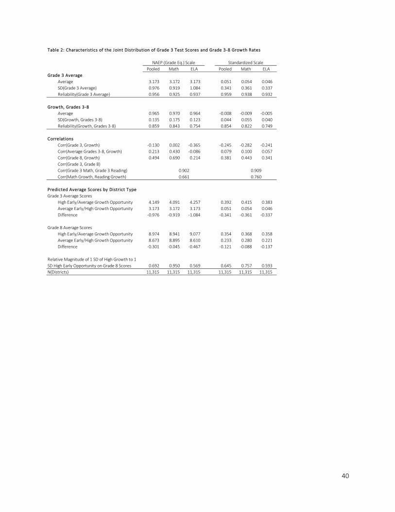
40

Pooled Math ELA Pooled Math ELAGrade 3 Average

Average 3.173 3.172 3.173 0.051 0.054 0.046SD(Grade 3 Average) 0.976 0.919 1.084 0.341 0.361 0.337Reliability(Grade 3 Average) 0.956 0.925 0.937 0.959 0.938 0.932

Growth, Grades 3-8Average 0.965 0.970 0.964 -0.008 -0.009 -0.005SD(Growth, Grades 3-8) 0.135 0.175 0.123 0.044 0.055 0.040Reliability(Growth, Grades 3-8) 0.859 0.843 0.754 0.854 0.822 0.749

CorrelationsCorr(Grade 3, Growth) -0.130 0.002 -0.365 -0.245 -0.282 -0.241Corr(Average Grades 3-8, Growth) 0.213 0.430 -0.086 0.079 0.100 0.057Corr(Grade 8, Growth) 0.494 0.690 0.214 0.381 0.443 0.341Corr(Grade 3, Grade 8)Corr(Grade 3 Math, Grade 3 Reading)Corr(Math Growth, Reading Growth)

Predicted Average Scores by District TypeGrade 3 Average Scores

High Early/Average Growth Opportunity 4.149 4.091 4.257 0.392 0.415 0.383Average Early/High Growth Opportunity 3.173 3.172 3.173 0.051 0.054 0.046Difference -0.976 -0.919 -1.084 -0.341 -0.361 -0.337

Grade 8 Average ScoresHigh Early/Average Growth Opportunity 8.974 8.941 9.077 0.354 0.368 0.358Average Early/High Growth Opportunity 8.673 8.895 8.610 0.233 0.280 0.221Difference -0.301 -0.045 -0.467 -0.121 -0.088 -0.137

0.692 0.950 0.569 0.645 0.757 0.593N(Districts) 11,315 11,315 11,315 11,315 11,315 11,315

Relative Magnitude of 1 SD of High Growth to 1 SD High Early Opportunity on Grade 8 Scores

Table 2: Characteristics of the Joint Distribution of Grade 3 Test Scores and Grade 3-8 Growth Rates

NAEP (Grade Eq.) Scale Standardized Scale

0.9020.661

0.9090.760

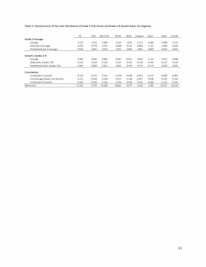
41

All Poor Non-Poor White Black Hispanic Asian Male FemaleGrade 3 Average

Average 3.173 2.351 3.803 3.535 1.933 2.177 4.286 3.088 3.274SD(Grade 3 Average) 0.976 0.779 0.791 0.808 0.762 0.883 1.215 1.000 0.959Reliability(Grade 3 Average) 0.956 0.901 0.913 0.931 0.899 0.881 0.899 0.943 0.941

Growth, Grades 3-8Average 0.965 0.942 0.985 0.967 0.912 0.992 1.110 0.932 0.998SD(Growth, Grades 3-8) 0.135 0.134 0.133 0.131 0.131 0.134 0.144 0.137 0.129Reliability(Growth, Grades 3-8) 0.859 0.809 0.811 0.831 0.796 0.770 0.719 0.829 0.819

CorrelationsCorr(Grade 3, Growth) -0.130 -0.475 -0.167 -0.148 -0.298 -0.431 0.273 -0.089 -0.087Corr(Average Grades 3-8, Growth) 0.213 -0.050 0.248 0.251 0.138 -0.057 0.508 0.245 0.242Corr(Grade 8, Growth) 0.494 0.403 0.563 0.556 0.509 0.341 0.668 0.512 0.505

N(Districts) 11,315 9,735 10,180 10,662 3,077 4,102 1,789 10,327 10,233

Table 3: Characteristics of the Joint Distribution of Grade 3 Test Scores and Grade 3-8 Growth Rates, by Subgroup

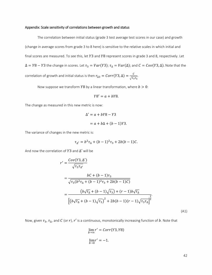
42

Appendix: Scale sensitivity of correlations between growth and status

The correlation between initial status (grade 3 test average test scores in our case) and growth

(change in average scores from grade 3 to 8 here) is sensitive to the relative scales in which initial and

final scores are measured. To see this, let 𝑌𝑌3 and 𝑌𝑌8 represent scores in grade 3 and 8, respectively. Let

∆ = 𝑌𝑌8 − 𝑌𝑌3 the change in scores. Let 𝜏𝜏3 = 𝑀𝑀𝑦𝑦𝑜𝑜(𝑌𝑌3); 𝜏𝜏∆ = 𝑀𝑀𝑦𝑦𝑜𝑜(∆); and 𝐶𝐶 = 𝐶𝐶𝑐𝑐𝑣𝑣(𝑌𝑌3,∆). Note that the

correlation of growth and initial status is then 𝑜𝑜∆3 = 𝐶𝐶𝑐𝑐𝑜𝑜𝑜𝑜(𝑌𝑌3,∆) = 𝐶𝐶�𝜏𝜏3𝜏𝜏∆

.

Now suppose we transform 𝑌𝑌8 by a linear transformation, where 𝑏𝑏 > 0:

𝑌𝑌8′ = 𝑦𝑦 + 𝑏𝑏𝑌𝑌8.

The change as measured in this new metric is now:

∆′ = 𝑦𝑦 + 𝑏𝑏𝑌𝑌8 − 𝑌𝑌3

= 𝑦𝑦 + 𝑏𝑏∆ + (𝑏𝑏 − 1)𝑌𝑌3.

The variance of changes in the new metric is:

𝜏𝜏∆′ = 𝑏𝑏2𝜏𝜏∆ + (𝑏𝑏 − 1)2𝜏𝜏3 + 2𝑏𝑏(𝑏𝑏 − 1)𝐶𝐶.

And now the correlation of 𝑌𝑌3 and ∆′ will be

𝑜𝑜′ =𝐶𝐶𝑐𝑐𝑣𝑣(𝑌𝑌3,∆′)

�𝜏𝜏3𝜏𝜏∆′

=𝑏𝑏𝐶𝐶 + (𝑏𝑏 − 1)𝜏𝜏3

�𝜏𝜏3(𝑏𝑏2𝜏𝜏∆ + (𝑏𝑏 − 1)2𝜏𝜏3 + 2𝑏𝑏(𝑏𝑏 − 1)𝐶𝐶)

=�𝑏𝑏√𝜏𝜏∆ + (𝑏𝑏 − 1)�𝜏𝜏3� + (𝑜𝑜 − 1)𝑏𝑏√𝜏𝜏∆

��𝑏𝑏√𝜏𝜏∆ + (𝑏𝑏 − 1)�𝜏𝜏3�2

+ 2𝑏𝑏(𝑏𝑏 − 1)(𝑜𝑜 − 1)�𝜏𝜏3𝜏𝜏∆�12

.

(A1)

Now, given 𝜏𝜏3, 𝜏𝜏∆, and 𝐶𝐶 (or 𝑜𝑜), 𝑜𝑜′ is a continuous, monotonically increasing function of 𝑏𝑏. Note that

lim𝑏𝑏→∞

𝑜𝑜′ = 𝐶𝐶𝑐𝑐𝑜𝑜𝑜𝑜(𝑌𝑌3,𝑌𝑌8)

lim𝑏𝑏→0

𝑜𝑜′ = −1.

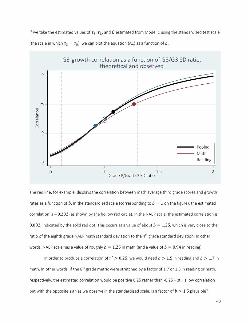
43

If we take the estimated values of 𝜏𝜏3, 𝜏𝜏∆, and 𝐶𝐶 estimated from Model 1 using the standardized test scale

(the scale in which 𝜏𝜏3 = 𝜏𝜏8), we can plot the equation (A1) as a function of 𝑏𝑏.

The red line, for example, displays the correlation between math average third grade scores and growth

rates as a function of 𝑏𝑏. In the standardized scale (corresponding to 𝑏𝑏 = 1 on the figure), the estimated

correlation is −0.282 (as shown by the hollow red circle). In the NAEP scale, the estimated correlation is

0.002, indicated by the solid red dot. This occurs at a value of about 𝑏𝑏 = 1.25, which is very close to the

ratio of the eighth grade NAEP math standard deviation to the 4th grade standard deviation. In other

words, NAEP scale has a value of roughly 𝑏𝑏 = 1.25 in math (and a value of 𝑏𝑏 = 0.94 in reading).

In order to produce a correlation of 𝑜𝑜′ > 0.25, we would need 𝑏𝑏 > 1.5 in reading and 𝑏𝑏 > 1.7 in

math. In other words, if the 8th grade metric were stretched by a factor of 1.7 or 1.5 in reading or math,

respectively, the estimated correlation would be positive 0.25 rather than -0.25 – still a low correlation

but with the opposite sign as we observe in the standardized scale. Is a factor of 𝑏𝑏 > 1.5 plausible?

44

One way to assess this is to examine other vertically scaled tests. Dadey and Briggs (2012)

examine 16 vertically scaled tests used in state assessment programs. For these tests, the value of 𝑏𝑏—the

ratio of the 8th grade standard deviation of scores to the 3rd grade standard deviation—ranges from 0.6 to

almost 1.3 (though most of the reading ratios are between 0.8 and 1.0; most of the math ratios are

between 0.9 and 1.1). Bloom et al (2008) report standard deviations for 7 vertically equated reading

tests; the grade 8 to grade 3 standard deviation ratios in those tests range from 0.87 to 1.04. Of the 23

vertically scaled assessments for which data are available, none have 𝑏𝑏 > 1.3. The vertical grey dashed

lines in the Figure show the range of values of 𝑏𝑏 reported by Dadey and Briggs and Bloom et al. The

possible correlations these values of 𝑏𝑏 would produce in the SEDA data range from −0.80 to +0.15. This

suggests that there is no plausible vertical scale that would yield a moderate or high positive correlation

between grade three test scores and growth rates.