EE 685 presentation

Optimization Flow Control,

I: Basic Algorithm and ConvergenceBy Steven Low and David Lapsley

Objective of the paper

Propose an optimization approach for flow control on a network whose resources are shared by a set of S of sources

Maximization of aggregate source utility over transmission rates is aimed

Sources select transmission rates that maximize their benefit (utility – bandwidth cost)

Synchronous and asynchronous distributed algorithms for converging optimal behavior in static environment is presented

Problem Framework

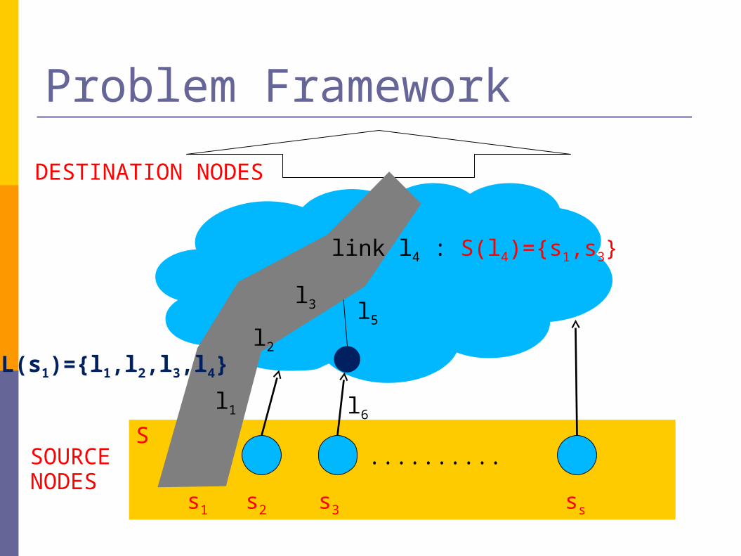
The problem is formulated for A network that consists of a set L of unidirectional links of capacities c l,

where l is element of L.

The network is shared by a set S of sources, where source s is characterized by a utility function Us(xs) that is concave increasing in its transmission rate xs

. The goal is to calculate source rates that maximize the sum of the

utilities ∑s ϵ S Us(xs) over xs subject to capacity constraints.

S

Problem Framework

s1 s2 s3 ss

..........

DESTINATION NODES

SOURCE NODES

L(s1)={l1,l2,l3,l4}

link l4 : S(l4)={s1,s3}

l1

l2

l3 l5

l6

Centralized optimization : Why not

Centralized optimization of source rates is possible in theory but not feasible and practical in real networks as

Knowledge of all utility functions are required Resource usage is coupled due to shared links. So all the sources should be

coordinated simultaneously

Therefore a distributed and decentralized approach is needed.

The value of the optimization frame-work presented

It is not always critical or feasible to attain exact optimality in a flow control problem

However the optimal framework acts as a guideline to shape the network dynamics to a desirable operating point where source utilities and resource costs are taken into consideration

Optimization frameworks may be used to refine and ameliorate practical flow control schemes

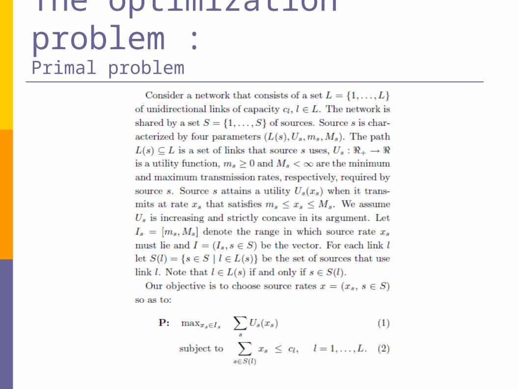
The optimization problem :Primal problem

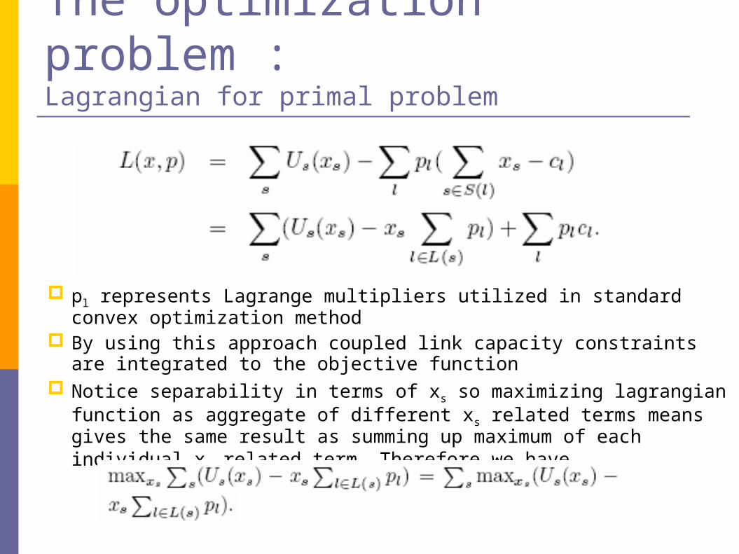
The optimization problem :Lagrangian for primal problem

pl represents Lagrange multipliers utilized in standard convex optimization method

By using this approach coupled link capacity constraints are integrated to the objective function

Notice separability in terms of xs so maximizing lagrangian function as aggregate of different xs related terms means gives the same result as summing up maximum of each individual xs related term. Therefore we have

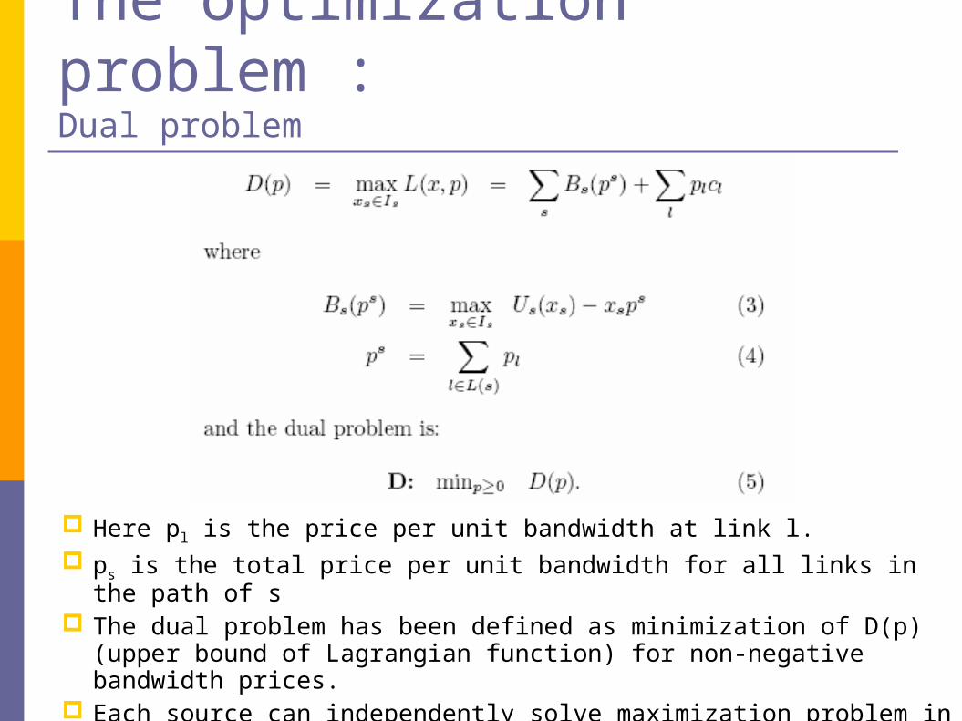
The optimization problem :Dual problem

Here pl is the price per unit bandwidth at link l. ps is the total price per unit bandwidth for all links in the path of s The dual problem has been defined as minimization of D(p) (upper bound of

Lagrangian function) for non-negative bandwidth prices. Each source can independently solve maximization problem in (3) for a given p

The optimization problem :Concavity and duality gap

For each p, a unique maximizer denoted by xs(p) exists since Us (source utility function) is strictly concave

Concavity of Us and linear constraints for the primal problem guarantees that there is no duality gap and dual optimal prices exist in the form of Lagrange Multipliers

Once p* is obtained by solving the dual problem, the primal optimal source rates x*=x(p*) can be computed by individual sources s by solving (3)

Therefore given p* individual sources can solve (3) without any coordination (key concept for distributed algorithm)

So p* acts as a coordination signal that aligns individual and joint optimality for flow control problem

Notations and assumptions :

R11 R12 ... R1s

R21 R22 ... R2s

.... .... ... ...

Rl1 Rl2 ... Rls

R=

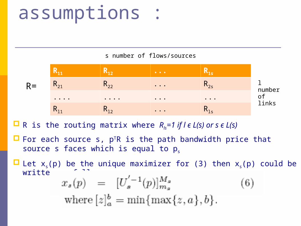
R is the routing matrix where Rls=1 if l ϵ L(s) or s ϵ L(s)

For each source s, pTR is the path bandwidth price that source s faces which is equal to ps

Let xs(p) be the unique maximizer for (3) then xs(p) could be written as follows :

s number of flows/sources

l number of links

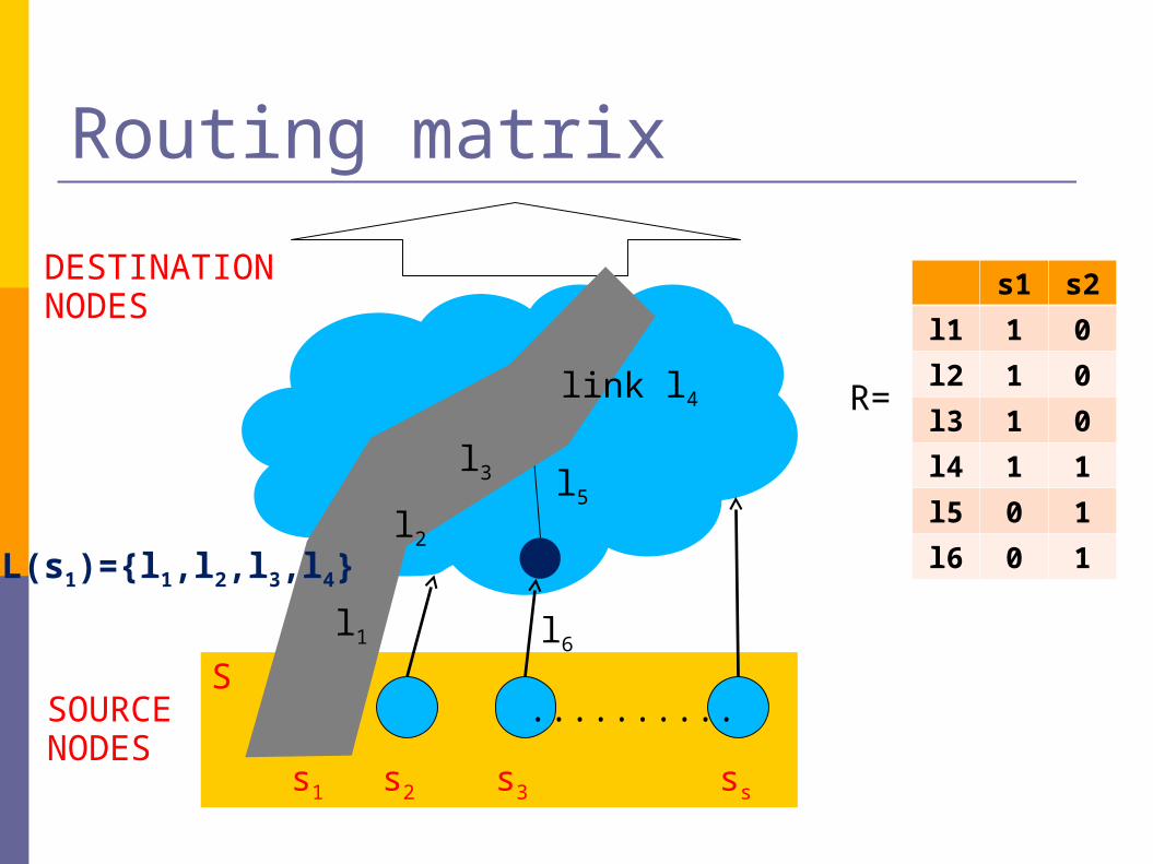
S

Routing matrix

s1 s2 s3 ss

..........

DESTINATION NODES

SOURCE NODES

L(s1)={l1,l2,l3,l4}

link l4

l1

l2

l3 l5

l6

s1 s2

l1 1 0

l2 1 0

l3 1 0

l4 1 1

l5 0 1

l6 0 1

R=

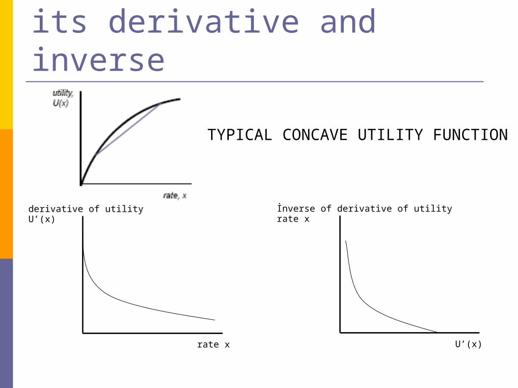
Concave utility function: its derivative and inverse

derivative of utility U’(x)

rate x

İnverse of derivative of utility rate x

U’(x)

TYPICAL CONCAVE UTILITY FUNCTION

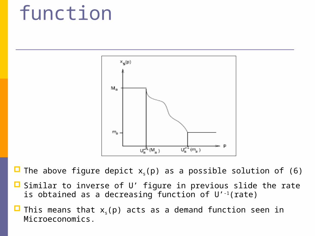
Source rate as demand function

The above figure depict xs(p) as a possible solution of (6)

Similar to inverse of U’ figure in previous slide the rate is obtained as a decreasing function of U’-1(rate)

This means that xs(p) acts as a demand function seen in Microeconomics.

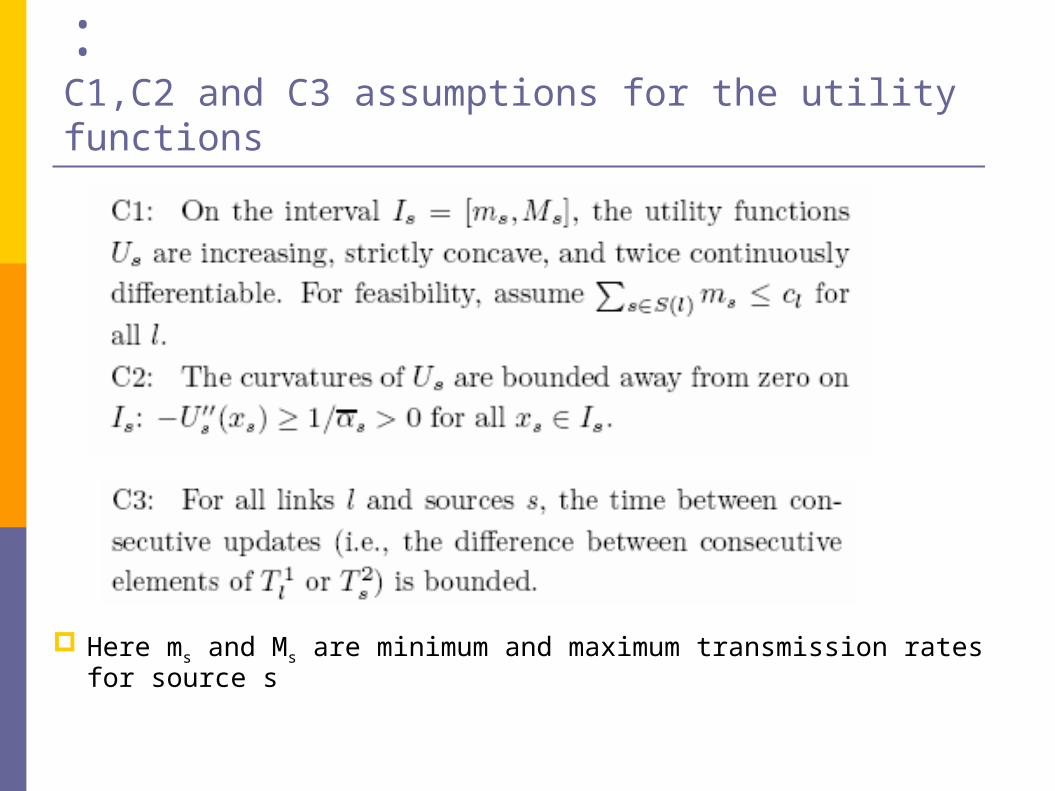
Fundamental assumptions :C1,C2 and C3 assumptions for the utility functions

Here ms and Ms are minimum and maximum transmission rates for source s

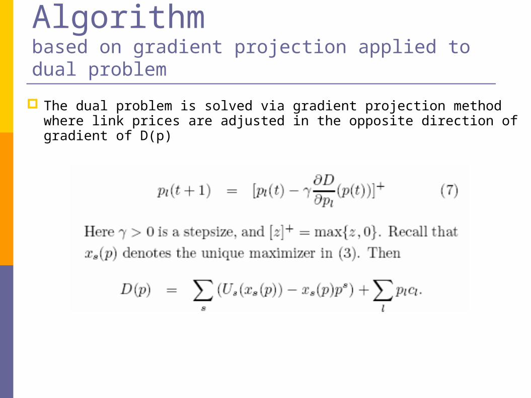
The dual problem is solved via gradient projection method where link prices are adjusted in the opposite direction of gradient of D(p)

Synchronous Distributed Algorithmbased on gradient projection applied to dual problem

Synchronous Distributed Algorithm

based on gradient projection appliedd to dual problem

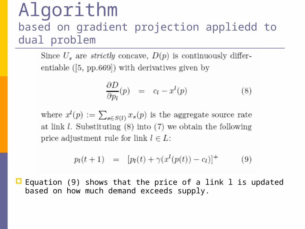
Equation (9) shows that the price of a link l is updated based on how much demand exceeds supply.

Synchronous Distributed AlgorithmGeneric outline of the algorithm

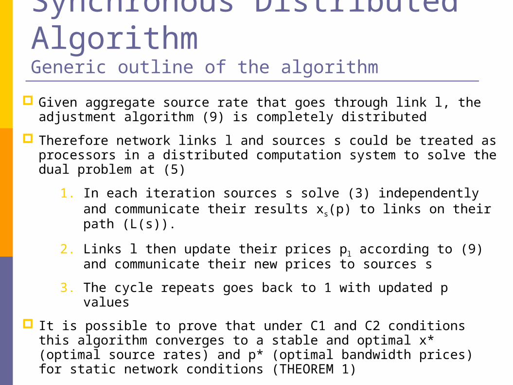
Given aggregate source rate that goes through link l, the adjustment algorithm (9) is completely distributed

Therefore network links l and sources s could be treated as processors in a distributed computation system to solve the dual problem at (5)

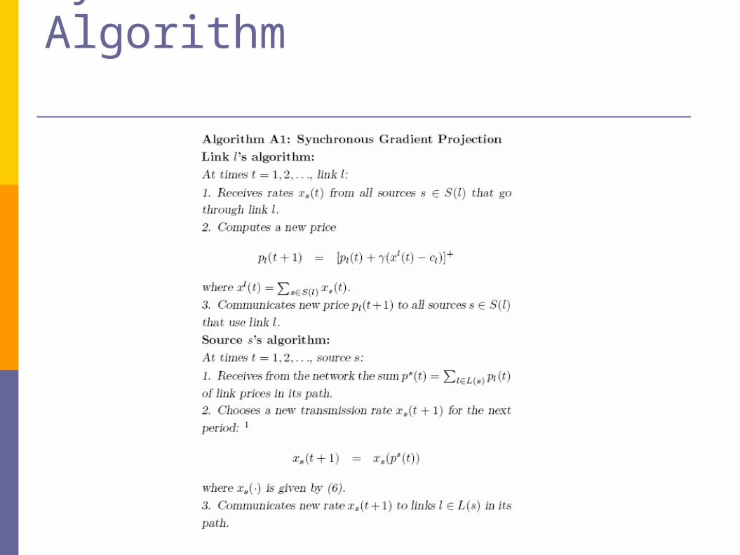
1. In each iteration sources s solve (3) independently and communicate their results xs(p) to links on their path (L(s)).

2. Links l then update their prices pl according to (9) and communicate their new prices to sources s

3. The cycle repeats goes back to 1 with updated p values

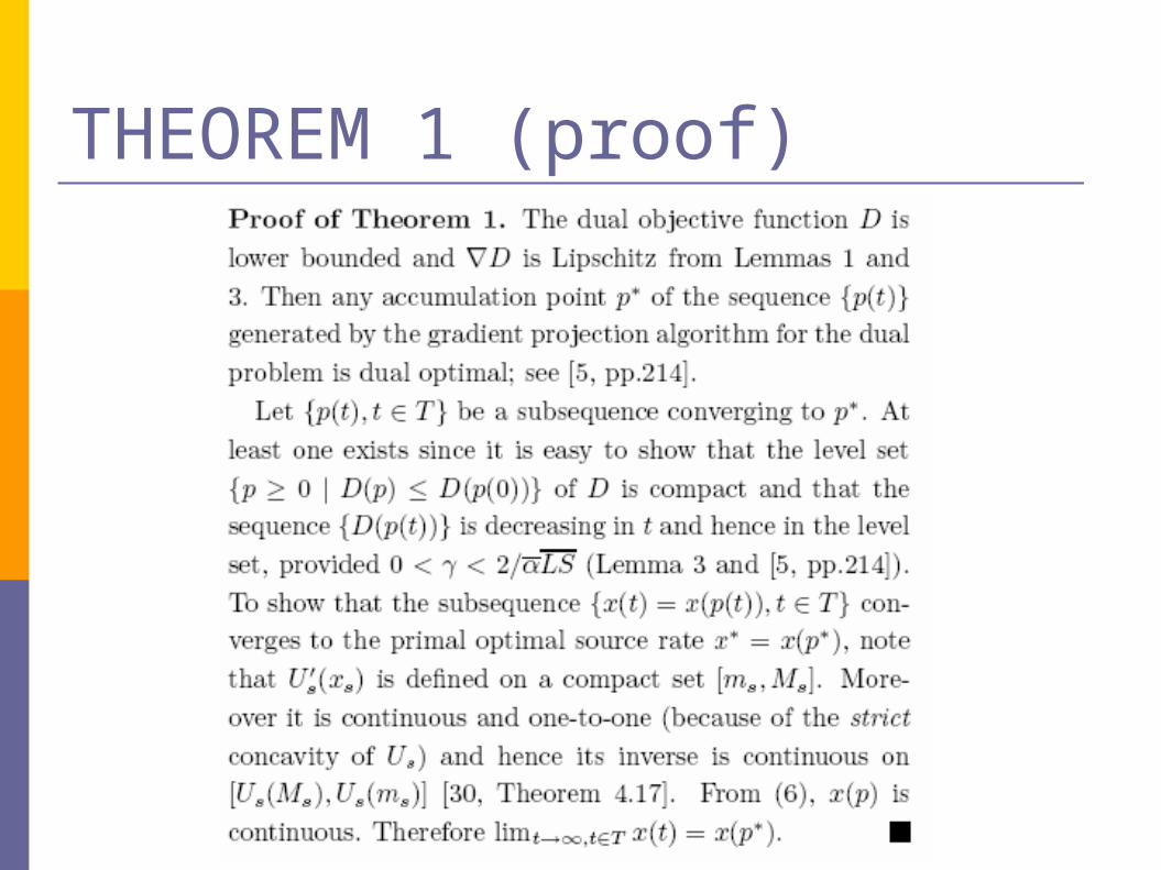
It is possible to prove that under C1 and C2 conditions this algorithm converges to a stable and optimal x* (optimal source rates) and p* (optimal bandwidth prices) for static network conditions (THEOREM 1)

Synchronous Distributed Algorithm

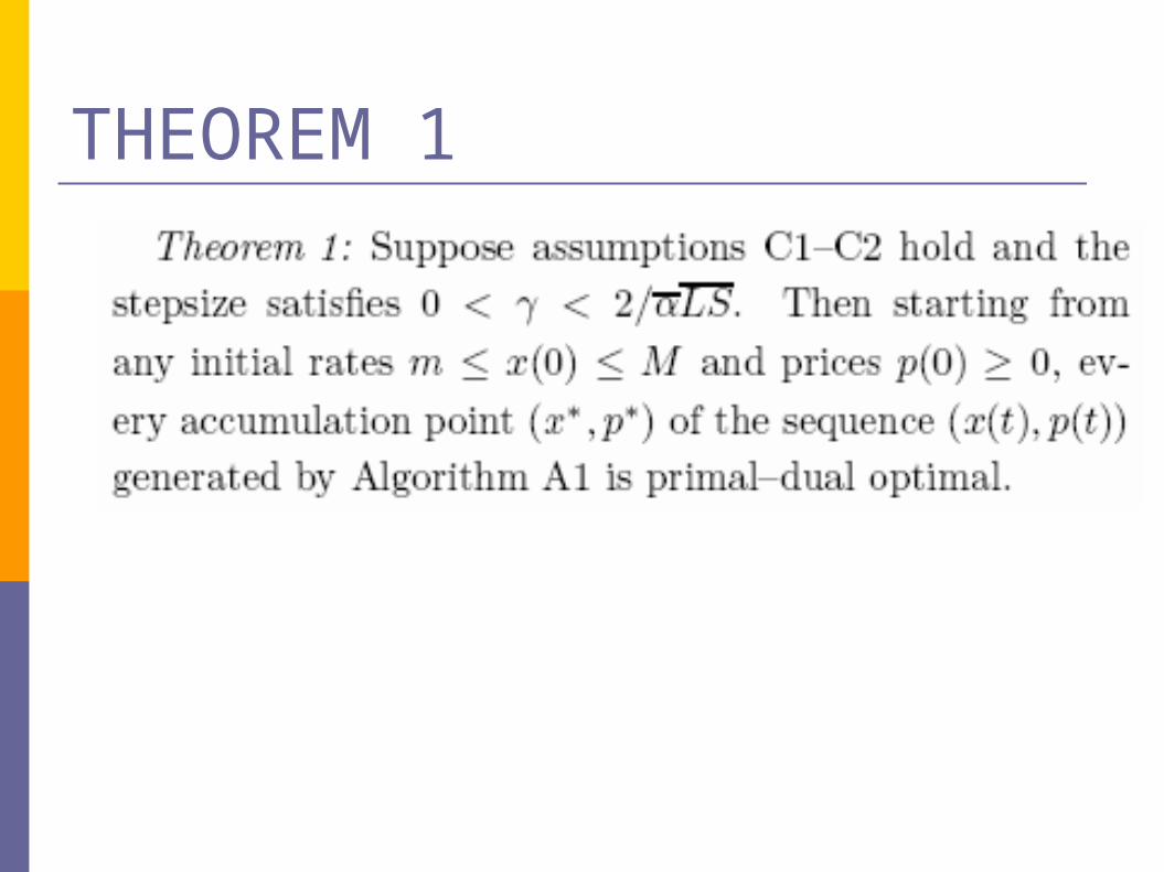
THEOREM 1

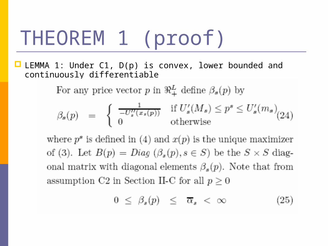
THEOREM 1 (proof) LEMMA 1: Under C1, D(p) is convex, lower bounded and continuously

differentiable

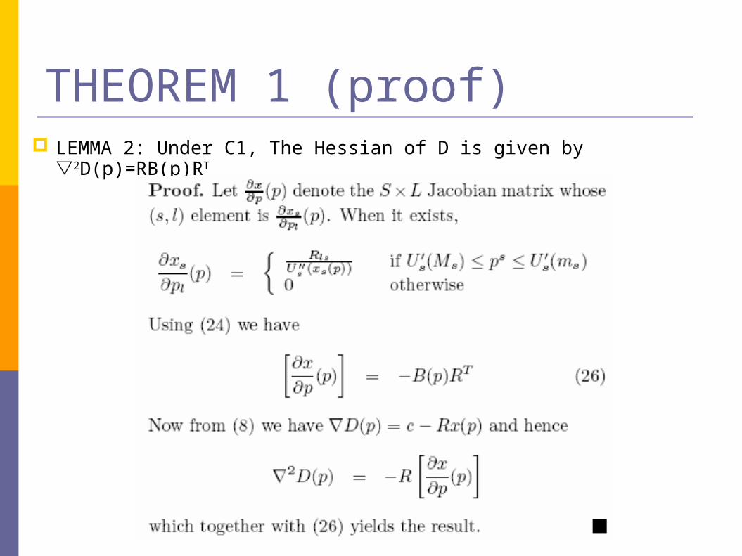
THEOREM 1 (proof) LEMMA 2: Under C1, The Hessian of D is given by 2D(p)=RB(p)RT

THEOREM 1 (proof)

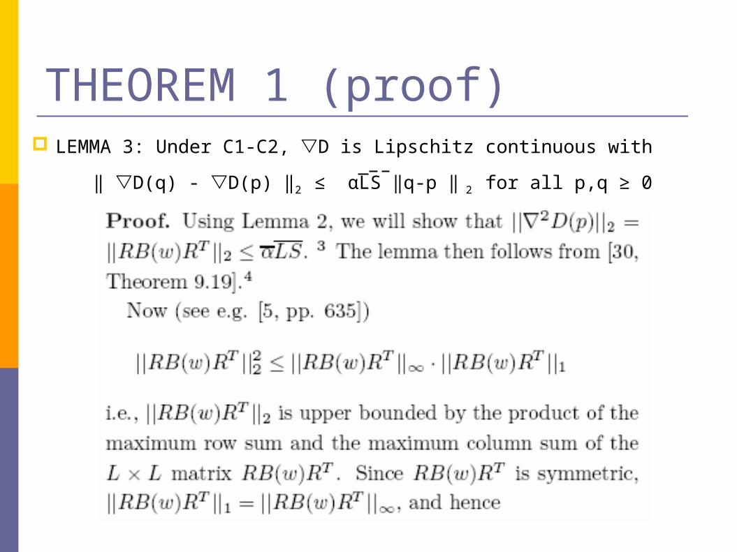
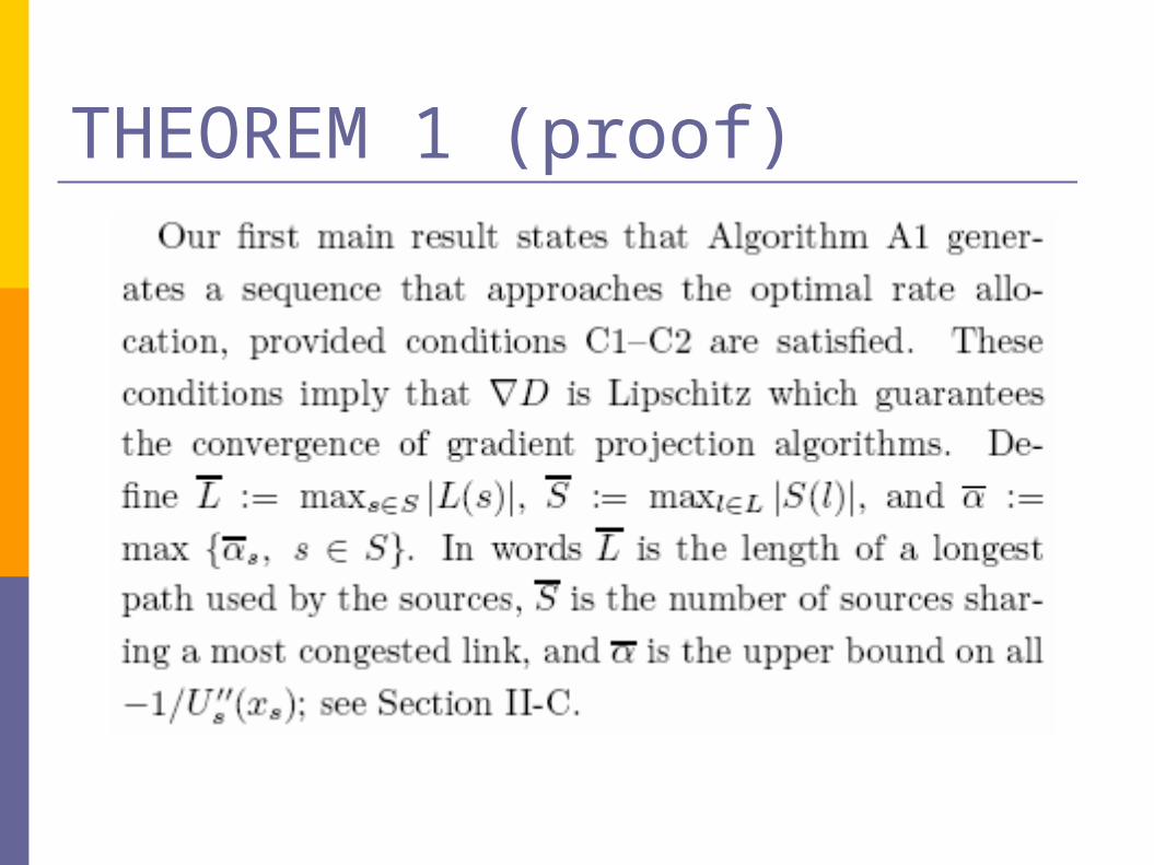
THEOREM 1 (proof) LEMMA 3: Under C1-C2, D is Lipschitz continuous with

‖ D(q) - D(p) ‖2 ≤ αLS ‖q-p ‖ 2 for all p,q ≥ 0

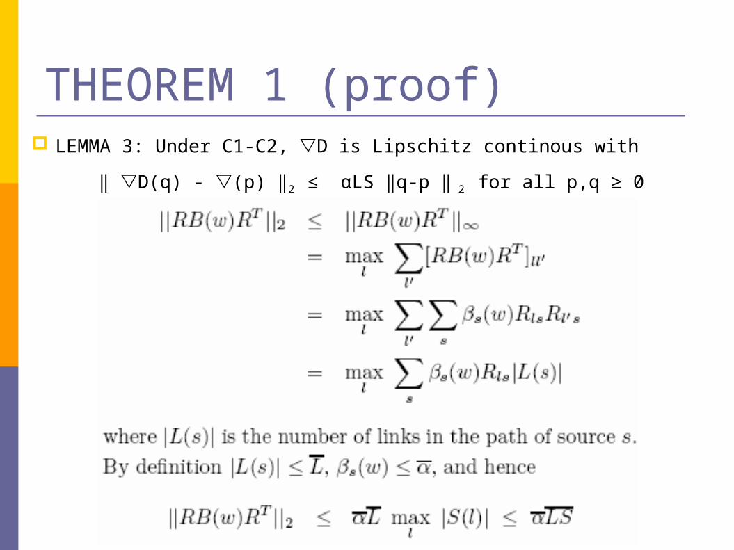
THEOREM 1 (proof) LEMMA 3: Under C1-C2, D is Lipschitz continous with

‖ D(q) - (p) ‖2 ≤ αLS ‖q-p ‖ 2 for all p,q ≥ 0

THEOREM 1 (proof)

Asynchronous Distributed Algorithm why asynchronous model is needed

The synchronous model of the last section assumes that updates at the sources and the links are synchronized

In realistic large network scenarios, synchronous updates might not be possible as

Sources may be located at different distances from the network links

.Network states (prices in our case) may be probed by different sources at different rates, e.g., the Resource Management

Feedbacks may reach different sources after different, and variable, delays.

These complications make our distributed computation system consisting of links and sources asynchronous.

The communication delays may be substantial and time-varying.

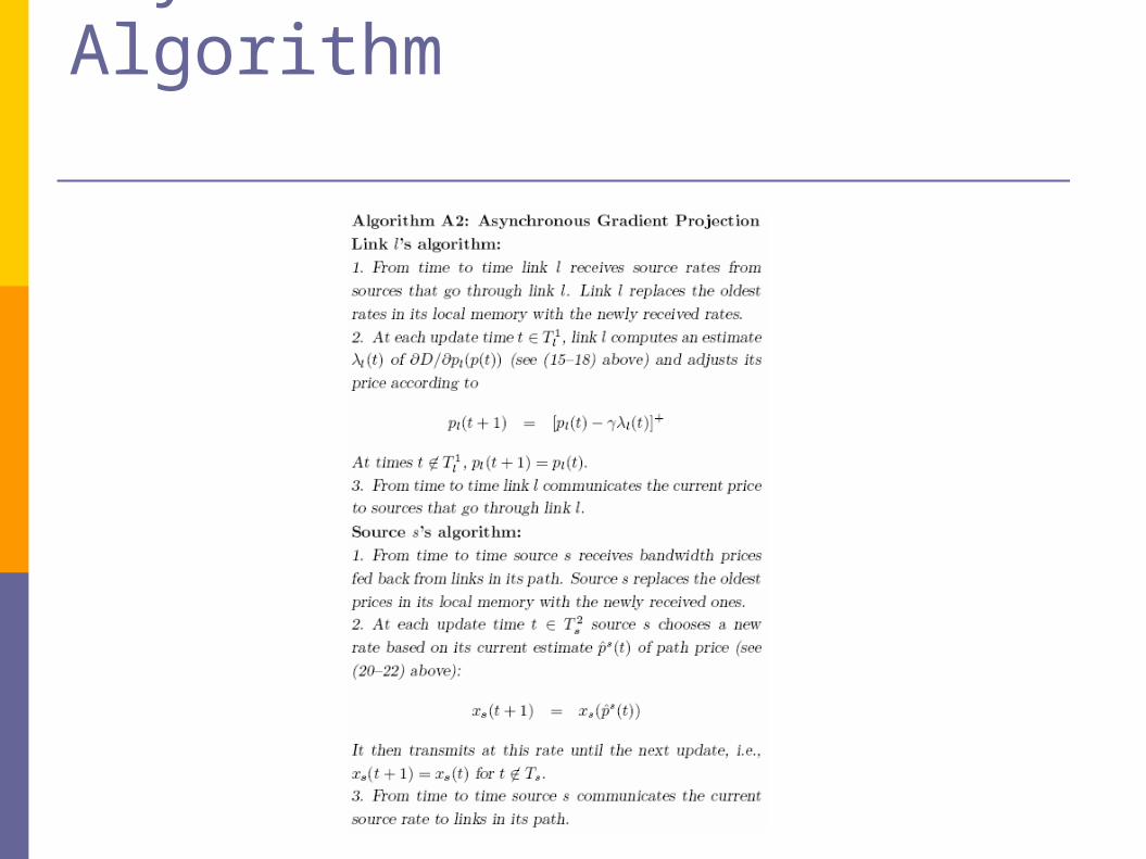
Asynchronous Distributed Algorithm

Generic outline of the algorithm

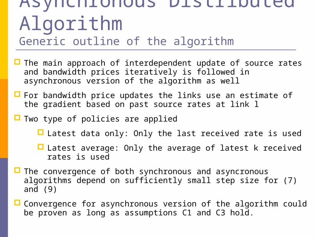
The main approach of interdependent update of source rates and bandwidth prices iteratively is followed in asynchronous version of the algorithm as well

For bandwidth price updates the links use an estimate of the gradient based on past source rates at link l

Two type of policies are applied

Latest data only: Only the last received rate is used

Latest average: Only the average of latest k received rates is used

The convergence of both synchronous and asyncronous algorithms depend on sufficiently small step size for (7) and (9)

Convergence for asynchronous version of the algorithm could be proven as long as assumptions C1 and C3 hold.

Asynchronous Distributed Algorithm

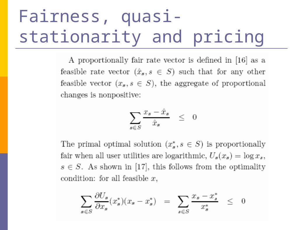
Fairness, quasi-stationarity and pricing

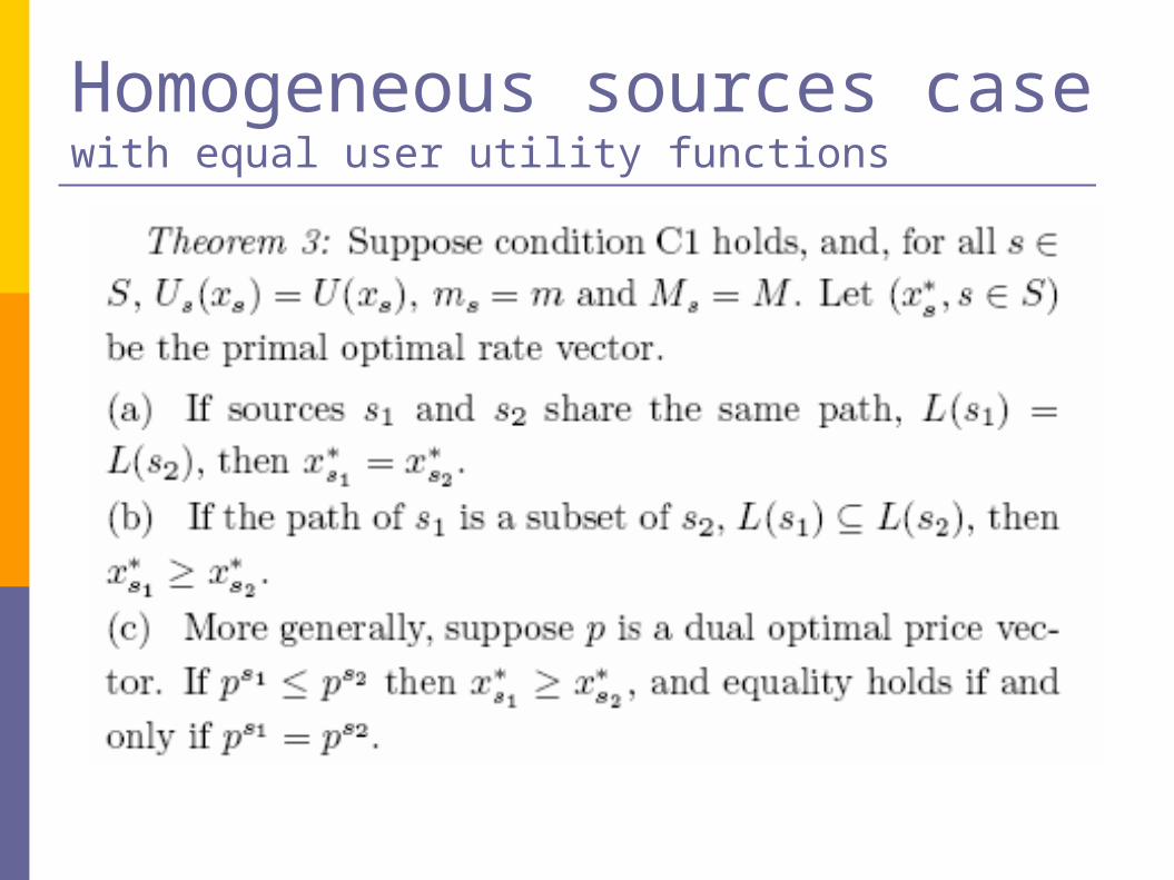
Homogeneous sources case with equal user utility functions

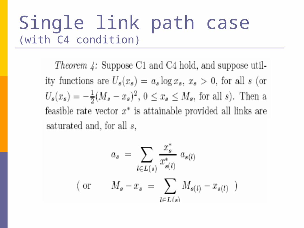
Single link path case(with C4 condition)

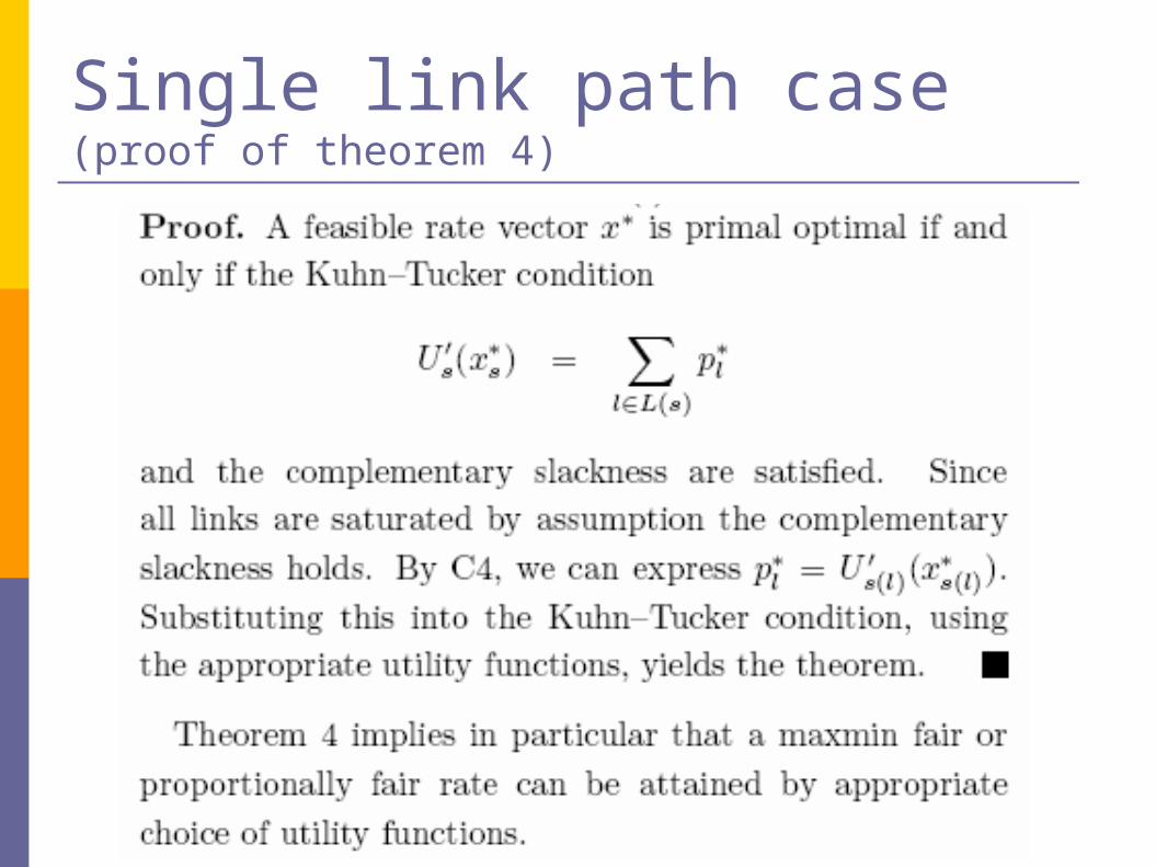
Single link path case(proof of theorem 4)