EE 741

Spring 2017

Primary and Secondary

Distribution System

One-Line Diagram of Typical Primary Distribution System

Radial-Type Primary Feeder

• Most common, simplest and lowest cost

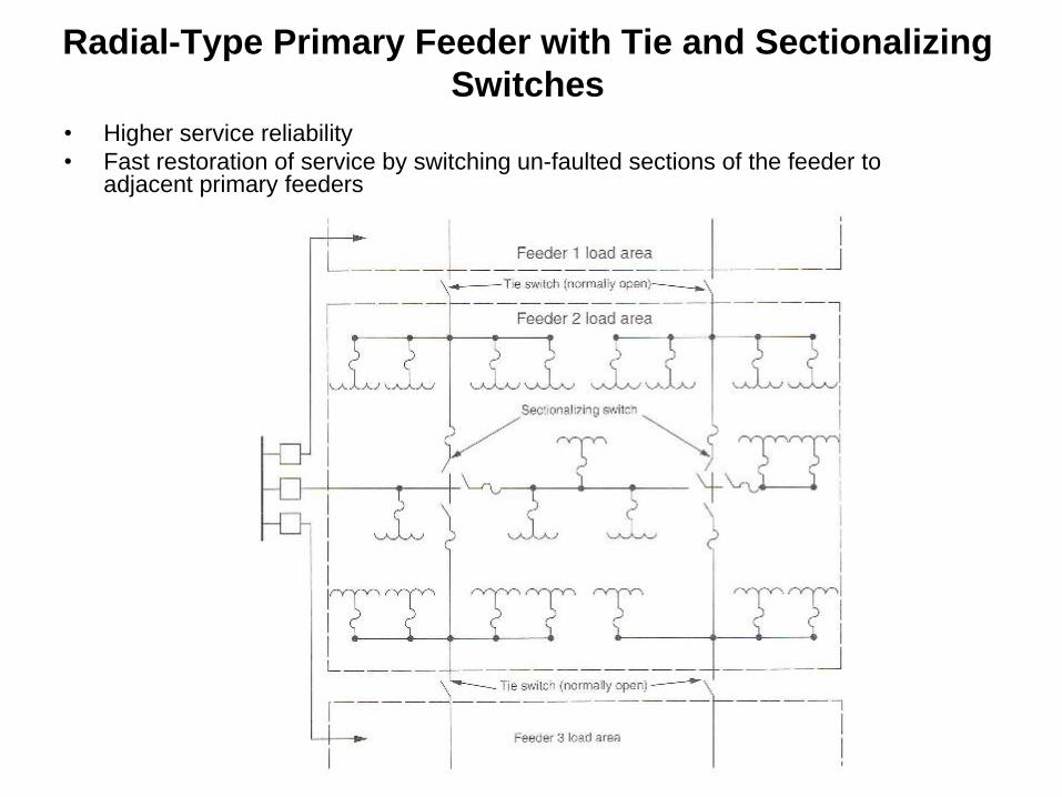
Radial-Type Primary Feeder with Tie and Sectionalizing

Switches

• Higher service reliability

• Fast restoration of service by switching un-faulted sections of the feeder to adjacent primary feeders

Radial-Type Primary with Express Feeder

Radial-Type Phase Area Feeder

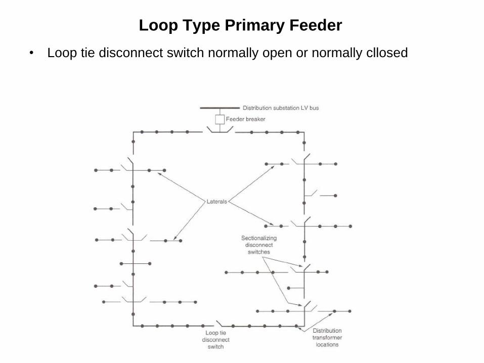
Loop Type Primary Feeder

• Loop tie disconnect switch normally open or normally cllosed

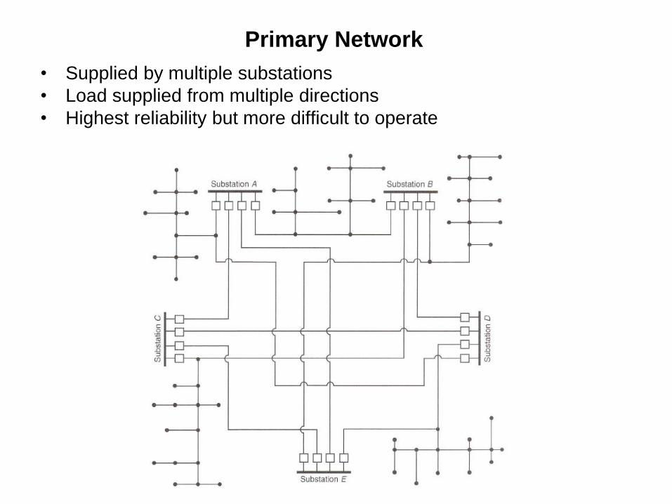
Primary Network

• Supplied by multiple substations

• Load supplied from multiple directions

• Highest reliability but more difficult to operate

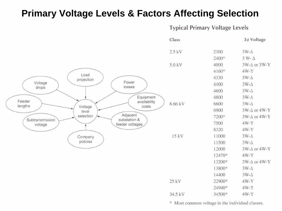
Primary Voltage Levels & Factors Affecting Selection

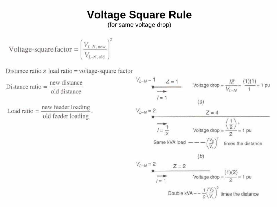
Voltage Square Rule (for same voltage drop)

Feeder Area Coverage Principle (if both dimensions of feeder service area change by the same proportion)

Factor Affecting Number of Feeders and Conductor Size

Selection

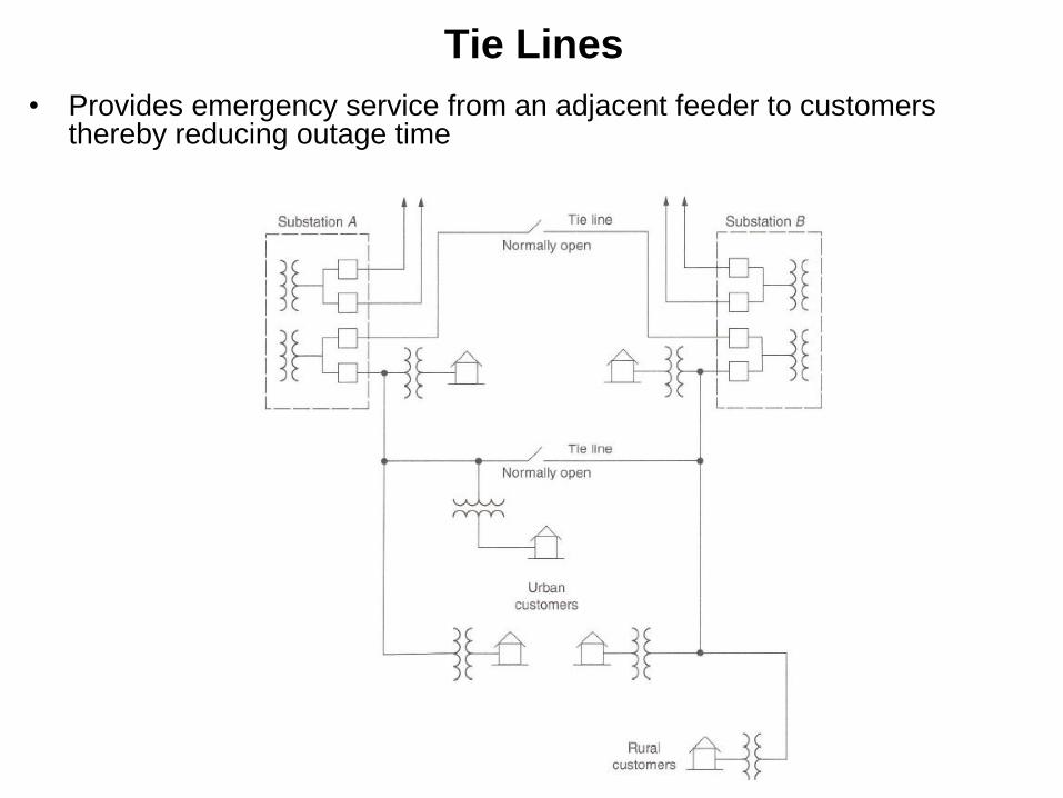
Tie Lines

• Provides emergency service from an adjacent feeder to customers thereby reducing outage time

Voltage drop and Power Loss in Radial Feeder with Uniformly

Distributed Load and Uniformly Increasing Load

2

15

8

3

2

sloss

s

rlIP

zlIVD

2

3

1

2

1

sloss

s

rlIP

zlIVD

Voltage drop and Power Loss in Radial Feeder with Uniformly

Distributed Load and Uniformly Increasing Load

Uniformly Distributed Load:

Uniformly Increasing Load:

Assignment # 1: Derive the following

Example of Overhead Primary Feeder Layout

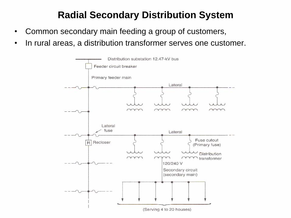
Radial Secondary Distribution System

• Common secondary main feeding a group of customers,

• In rural areas, a distribution transformer serves one customer.

Secondary Banking

• Secondary main served by multiple transformers (in parallel) that are

fed from the same primary feeder.

• Improved voltage regulation and service reliability, reduced voltage dip

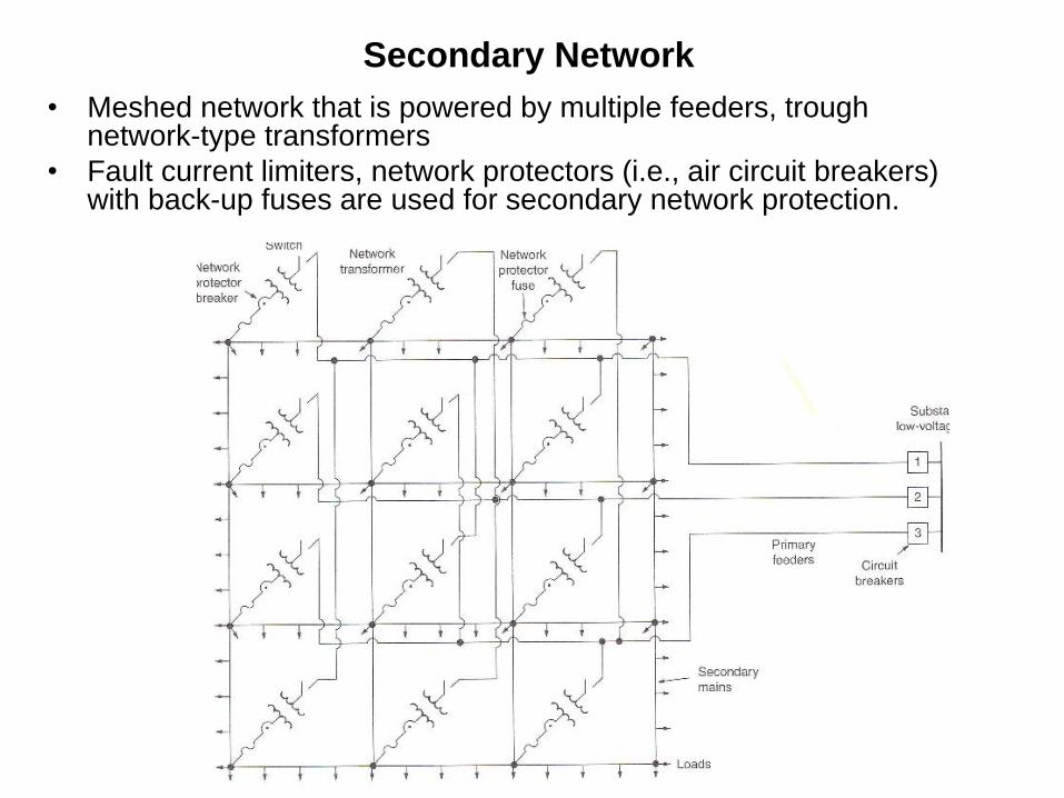
Secondary Network

• Meshed network that is powered by multiple feeders, trough network-type transformers

• Fault current limiters, network protectors (i.e., air circuit breakers) with back-up fuses are used for secondary network protection.

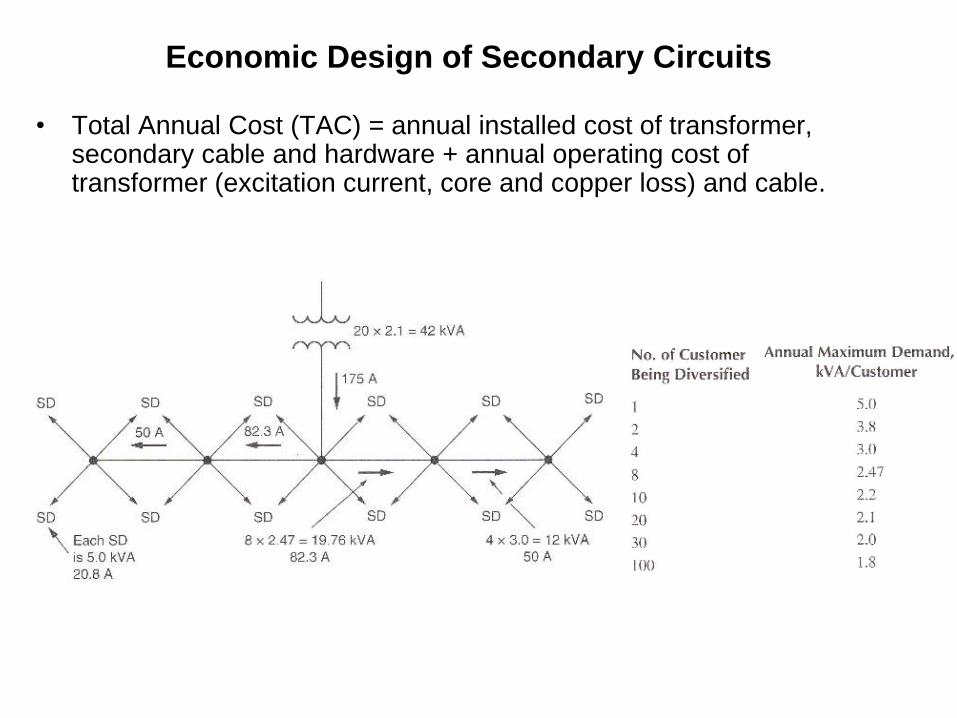
Economic Design of Secondary Circuits

• Total Annual Cost (TAC) = annual installed cost of transformer,

secondary cable and hardware + annual operating cost of transformer (excitation current, core and copper loss) and cable.

Series impedance of transmission lines

• Consists of the resistance of the conductors and the self

and mutual inductive reactances resulting from the

magnetic field surrounding the conductors.

• In the transmission system, the lines are often

transposed and equally loaded. Hence the self and

mutual reactances can be combined to form the phase

reactance.

• In a 60 Hz system,

• Distribution lines are rarely if ever transposed.

Additionally, the load is often unbalanced. Hence, it is

necessary to retain the identity of the self and mutual

reactances and take into account the ground return path

of the unbalanced currents.

• In a 60 Hz system, with earth resistivity of 100 Ω-m, the

self and mutual impedance of conductor i are

approximated using the modified Carson’s equations.

Series impedance of distribution lines

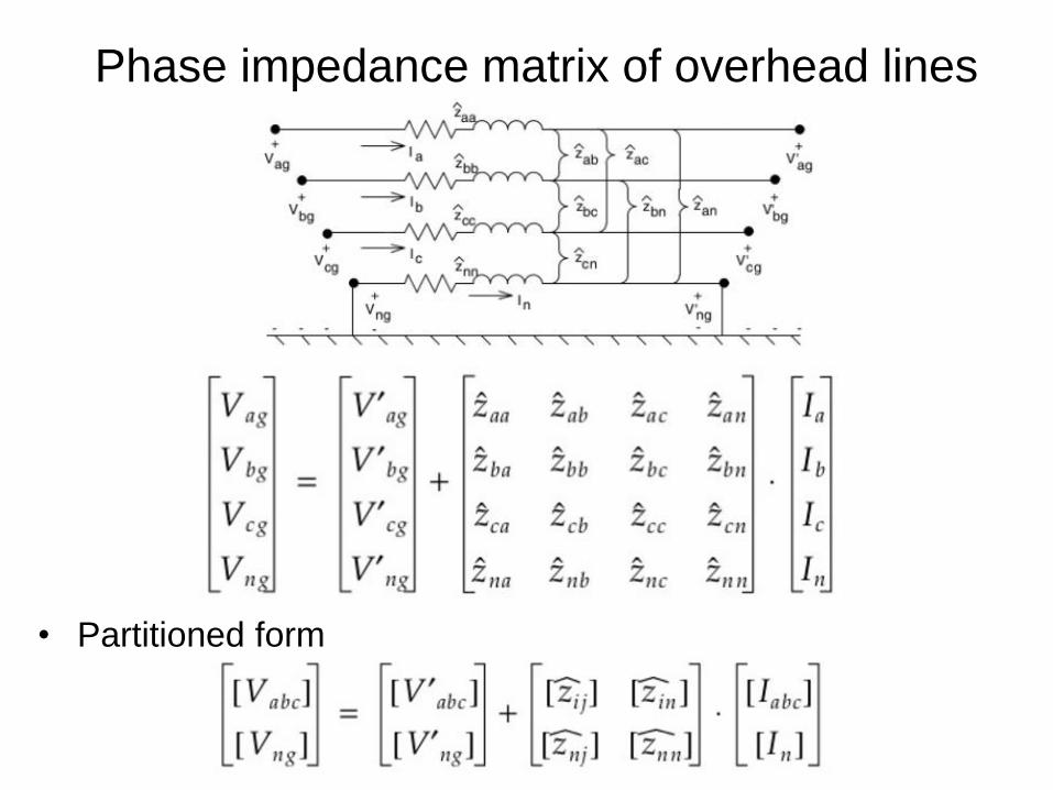
Phase impedance matrix of overhead lines

• Partitioned form

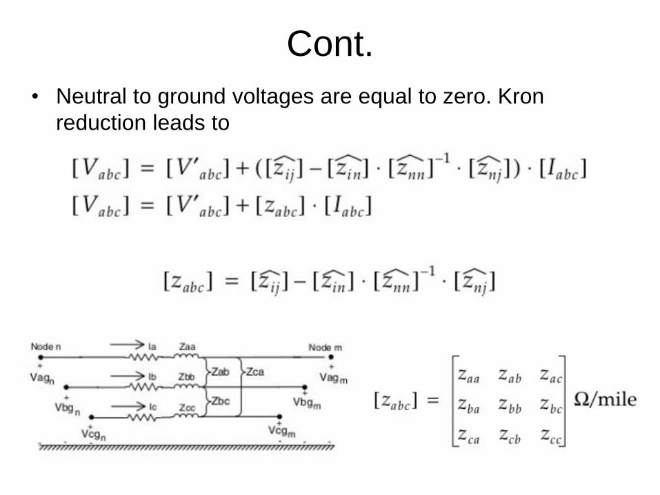
Cont.

• Neutral to ground voltages are equal to zero. Kron

reduction leads to

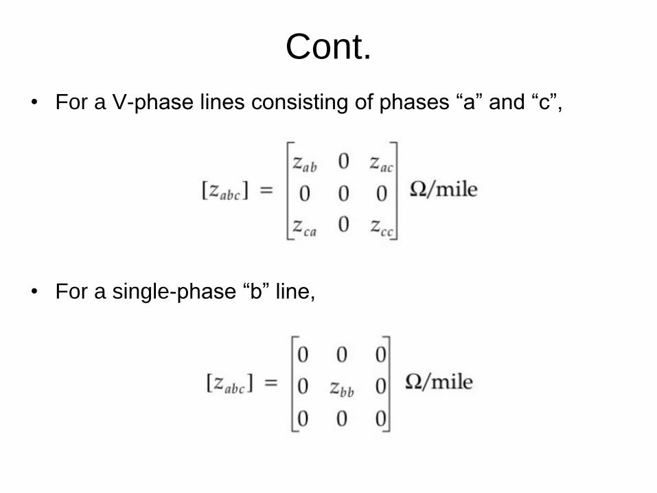
Cont.

• For a V-phase lines consisting of phases “a” and “c”,

• For a single-phase “b” line,

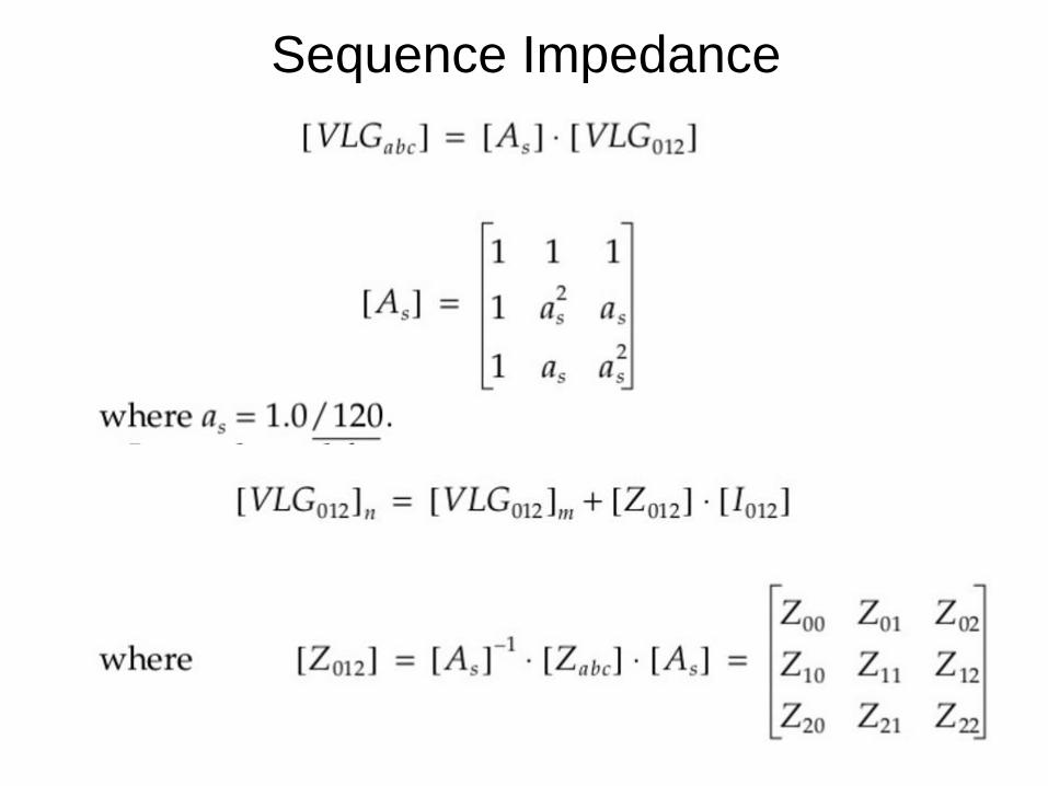
Sequence Impedance

Cont.

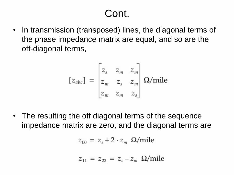
• In transmission (transposed) lines, the diagonal terms of

the phase impedance matrix are equal, and so are the

off-diagonal terms,

• The resulting the off diagonal terms of the sequence

impedance matrix are zero, and the diagonal terms are

Shunt Admittance of overhead lines

• The shunt admittance consists of the conductance which

is often very small, hence ignored, and the capacitance as

a result of the potential difference between conductors.

• Using the method of conductors and their images,

• Where

• Self and mutual potential coefficients:

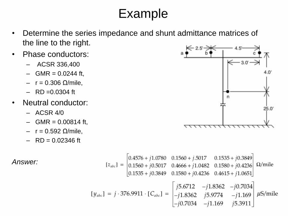
Example

• Determine the series impedance and shunt admittance matrices of

the line to the right.

• Phase conductors:

– ACSR 336,400

– GMR = 0.0244 ft,

– r = 0.306 Ω/mile,

– RD =0.0304 ft

• Neutral conductor:

– ACSR 4/0

– GMR = 0.00814 ft,

– r = 0.592 Ω/mile,

– RD = 0.02346 ft

Answer:

Series impedance and shunt admittance of

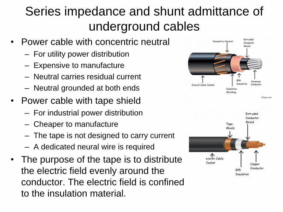
underground cables • Power cable with concentric neutral

– For utility power distribution

– Expensive to manufacture

– Neutral carries residual current

– Neutral grounded at both ends

• Power cable with tape shield

– For industrial power distribution

– Cheaper to manufacture

– The tape is not designed to carry current

– A dedicated neural wire is required

• The purpose of the tape is to distribute

the electric field evenly around the

conductor. The electric field is confined

to the insulation material.

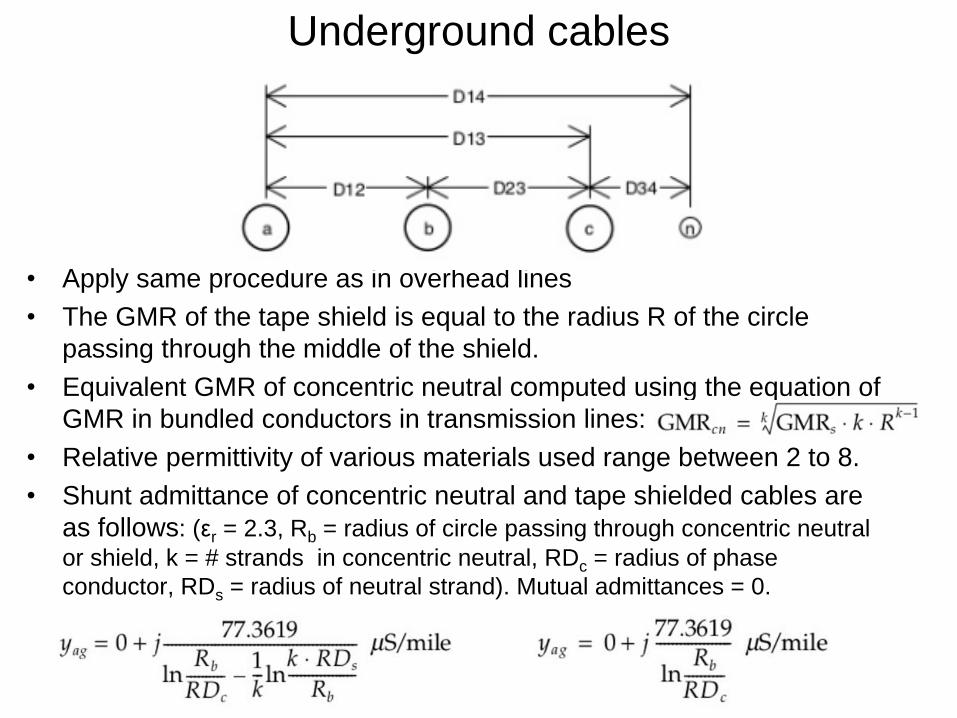
Underground cables

• Apply same procedure as in overhead lines

• The GMR of the tape shield is equal to the radius R of the circle

passing through the middle of the shield.

• Equivalent GMR of concentric neutral computed using the equation of

GMR in bundled conductors in transmission lines:

• Relative permittivity of various materials used range between 2 to 8.

• Shunt admittance of concentric neutral and tape shielded cables are

as follows: (εr = 2.3, Rb = radius of circle passing through concentric neutral

or shield, k = # strands in concentric neutral, RDc = radius of phase

conductor, RDs = radius of neutral strand). Mutual admittances = 0.

Distribution feeder model

Distribution feeder model

• Voltage unbalance (NEMA definition):

• Motor derating when voltage unbalance exceeds 1%.

• Simplified model (for short overhead lines with negligible

shunt admittance)

Assignment # 3

Consider the line configuration in the example. The line

length is 4 miles, and it serves a balanced 3 –phase load of

10 MVA @ 0.85 PF (lag). The voltages at the load are

balanced and equal to 13.2 kV.

1) Compute the line-to neutral voltages at the source end.

2) Compute the voltage unbalance at the source end.

3) Compute the real and reactive power supplied by the

source and the total power loss in the line.