Embed Size (px)
Citation preview

EE40 Summer 2006: Lecture 5 Instructor: Octavian Florescu 1
Announcements Lecture 3 updated on web. Slide 29
reversed dependent and independent sources.
Solution to PS1 on web today PS2 due next Tuesday at 6pm Midterm 1 Tuesday June18th 12:00-
1:30pm. Location TBD.

EE40 Summer 2006: Lecture 5 Instructor: Octavian Florescu 2
Review
Capacitors/InductorsVoltage/current relationshipStored Energy
1st Order CircuitsRL / RC circuitsSteady State / Transient responseNatural / Step response
EE40 Summer 2006: Lecture 5 Instructor: Octavian Florescu 3
Lecture #5OUTLINE
Chap 4 RC and RL Circuits with General Sources
Particular and complementary solutions Time constant
Second Order Circuits The differential equation Particular and complementary solutions The natural frequency and the damping ratio
Chap 5 Types of Circuit Excitation Why Sinusoidal Excitation? Phasors Complex Impedances
ReadingChap 4, Chap 5 (skip 5.7)
EE40 Summer 2006: Lecture 5 Instructor: Octavian Florescu 4
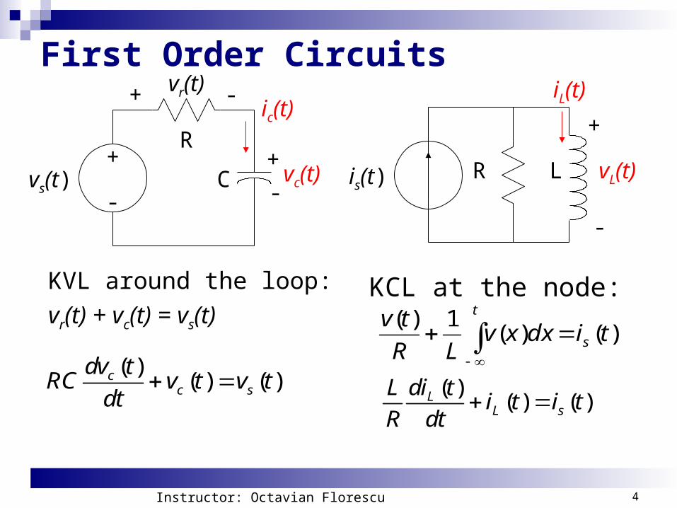
First Order Circuits
( )( ) ( )c
c s
dv tRC v t v t
dt
KVL around the loop:
vr(t) + vc(t) = vs(t)
R+
-Cvs(t)
+
-vc(t)
+ -vr(t)
vL(t)is(t) R L
+
-
)()(1)(
tidxxvLR
tvs
t
KCL at the node:
( )( ) ( )L
L s
di tLi t i t
R dt
ic(t)iL(t)

EE40 Summer 2006: Lecture 5 Instructor: Octavian Florescu 5
Complete Solution Voltages and currents in a 1st order circuit satisfy a differential
equation of the form
f(t) is called the forcing function. The complete solution is the sum of particular solution (forced
response) and complementary solution (natural response).
Particular solution satisfies the forcing function Complementary solution is used to satisfy the initial conditions. The initial conditions determine the value of K.
( )( ) ( )
dx tx t f t
dt
/
( )( ) 0
( )
cc
tc
dx tx t
dt
x t Ke
( )
( ) ( )pp
dx tx t f t
dt Homogeneous
equation
( ) ( ) ( )p cx t x t x t

EE40 Summer 2006: Lecture 5 Instructor: Octavian Florescu 6
The Time Constant The complementary solution for any 1st
order circuit is
For an RC circuit, = RC For an RL circuit, = L/R
/( ) tcx t Ke

EE40 Summer 2006: Lecture 5 Instructor: Octavian Florescu 7
What Does Xc(t) Look Like?
= 10-4/( ) tcx t e
• is the amount of time necessary for an exponential to decay to 36.7% of its initial value.
• -1/ is the initial slope of an exponential with an initial value of 1.

EE40 Summer 2006: Lecture 5 Instructor: Octavian Florescu 8
The Particular Solution The particular solution xp(t) is usually a
weighted sum of f(t) and its first derivative. If f(t) is constant, then xp(t) is constant.
If f(t) is sinusoidal, then xp(t) is sinusoidal.

EE40 Summer 2006: Lecture 5 Instructor: Octavian Florescu 9
Example
KVL:
R = 5kΩ
+
-C = 1uF
+
-vc(t)
+ -vr(t)ic(t)
t = 0
vs(t) = 2sin(200t)

EE40 Summer 2006: Lecture 5 Instructor: Octavian Florescu 10
2nd Order Circuits Any circuit with a single capacitor, a single
inductor, an arbitrary number of sources, and an arbitrary number of resistors is a circuit of order 2.
Any voltage or current in such a circuit is the solution to a 2nd order differential equation.

EE40 Summer 2006: Lecture 5 Instructor: Octavian Florescu 11
A 2nd Order RLC Circuit
R+
-Cvs(t)
i (t)
L
Application: FiltersA bandpass filter such as the IF amp for
the AM radio.A lowpass filter with a sharper cutoff than
can be obtained with an RC circuit.

EE40 Summer 2006: Lecture 5 Instructor: Octavian Florescu 12
The Differential Equation
KVL around the loop:
vr(t) + vc(t) + vl(t) = vs(t)
i (t)
R+
-Cvs(t)
+
-
vc(t)
+ -vr(t)
L
+- vl(t)
1 ( )( ) ( ) ( )
t
s
di tRi t i x dx L v t
C dt
2
2
( )( ) 1 ( ) 1( ) sdv tR di t d i t
i tL dt LC dt L dt

EE40 Summer 2006: Lecture 5 Instructor: Octavian Florescu 13
The Differential EquationThe voltage and current in a second order circuit is the solution to a differential equation of the following form:
Xp(t) is the particular solution (forced response) and Xc(t) is the complementary solution (natural response).
2202
( ) ( )2 ( ) ( )
d x t dx tx t f t
dt dt
( ) ( ) ( )p cx t x t x t

EE40 Summer 2006: Lecture 5 Instructor: Octavian Florescu 14
The Particular Solution The particular solution xp(t) is usually a
weighted sum of f(t) and its first and second derivatives.
If f(t) is constant, then xp(t) is constant.
If f(t) is sinusoidal, then xp(t) is sinusoidal.

EE40 Summer 2006: Lecture 5 Instructor: Octavian Florescu 15
The Complementary SolutionThe complementary solution has the following form:
K is a constant determined by initial conditions.s is a constant determined by the coefficients of the differential equation.
( ) stcx t Ke
2202
2 0st st
std Ke dKeKe
dt dt
2 202 0st st sts Ke sKe Ke
2 202 0s s

EE40 Summer 2006: Lecture 5 Instructor: Octavian Florescu 16
Characteristic Equation To find the complementary solution, we
need to solve the characteristic equation:
The characteristic equation has two roots-call them s1 and s2.
2 20 0
0
2 0s s
1 21 2( ) s t s t
cx t K e K e
21 0 0 1s
22 0 0 1s

EE40 Summer 2006: Lecture 5 Instructor: Octavian Florescu 17
Damping Ratio and Natural Frequency
The damping ratio determines what type of solution we will get:Exponentially decreasing ( >1)Exponentially decreasing sinusoid ( < 1)
The natural frequency is 0
It determines how fast sinusoids wiggle.
0
2
1 0 0 1s
22 0 0 1s damping ratio

EE40 Summer 2006: Lecture 5 Instructor: Octavian Florescu 18
Overdamped : Real Unequal Roots If > 1, s1 and s2 are real and not equal.
tt
c eKeKti
1
2
1
1
200
200
)(
0
0.2
0.4
0.6
0.8
1
-1.00E-06
t
i(t)
-0.2
0
0.2
0.4
0.6
0.8
-1.00E-06
t
i(t)

EE40 Summer 2006: Lecture 5 Instructor: Octavian Florescu 19
Underdamped: Complex Roots If < 1, s1 and s2 are complex. Define the following constants:
1 2( ) cos sintc d dx t e A t A t
0 20 1d
-1
-0.8
-0.6
-0.4
-0.2
0
0.2
0.4
0.6
0.8
1
-1.00E-05 1.00E-05 3.00E-05
t
i(t)

EE40 Summer 2006: Lecture 5 Instructor: Octavian Florescu 20
Critically damped: Real Equal Roots
If = 1, s1 and s2 are real and equal.
0 01 2( ) t t
cx t K e K te

EE40 Summer 2006: Lecture 5 Instructor: Octavian Florescu 21
Example
For the example, what are and 0?
dt
tdv
Lti
LCdt
tdi
L
R
dt
tid s )(1)(
1)()(2
2
22
0 02
( ) ( )2 ( ) 0c c
c
d x t dx tx t
dt dt
20 0
1, 2 ,
2
R R C
LC L L
10+
-769pF
i (t)
159H

EE40 Summer 2006: Lecture 5 Instructor: Octavian Florescu 22
Example = 0.011 0 = 2455000 Is this system over damped, under
damped, or critically damped? What will the current look like?
-1
-0.8
-0.6
-0.4
-0.2
0
0.2
0.4
0.6
0.8
1
-1.00E-05 1.00E-05 3.00E-05
t
i(t)

EE40 Summer 2006: Lecture 5 Instructor: Octavian Florescu 23
Slightly Different Example Increase the resistor to 1k What are and 0?
1k+
-769pFvs(t)
i (t)
159H
= 2455000
0
0.2
0.4
0.6
0.8
1
-1.00E-06
t
i(t)

EE40 Summer 2006: Lecture 5 Instructor: Octavian Florescu 24
Types of Circuit Excitation
Linear Time- Invariant Circuit
Steady-State Excitation
Linear Time- Invariant Circuit
OR
Linear Time- Invariant Circuit
DigitalPulseSource
Transient Excitations
Linear Time- Invariant Circuit
Sinusoidal (Single-Frequency) ExcitationAC Steady-State
(DC Steady-State)Step Excitation

EE40 Summer 2006: Lecture 5 Instructor: Octavian Florescu 25
Why is Single-Frequency Excitation Important? Some circuits are driven by a single-frequency sinusoidal
source. Some circuits are driven by sinusoidal sources whose
frequency changes slowly over time. You can express any periodic electrical signal as a sum
of single-frequency sinusoids – so you can analyze the response of the (linear, time-invariant) circuit to each individual frequency component and then sum the responses to get the total response.
• This is known as Fourier Transform and is tremendously important to all kinds of engineering disciplines!

EE40 Summer 2006: Lecture 5 Instructor: Octavian Florescu 26
a b
c d
sig
nal
sig
nal
Time (ms)
Frequency (Hz)
Sig
na
l (V
)
Re
lative
Am
plitu
de
Sig
na
l (V
)
Sig
na
l (V
)
Representing a Square Wave as a Sum of Sinusoids
(a)Square wave with 1-second period. (b) Fundamental component (dotted) with 1-second period, third-harmonic (solid black) with1/3-second period, and their sum (blue). (c) Sum of first ten components. (d) Spectrum with 20 terms.
EE40 Summer 2006: Lecture 5 Instructor: Octavian Florescu 27
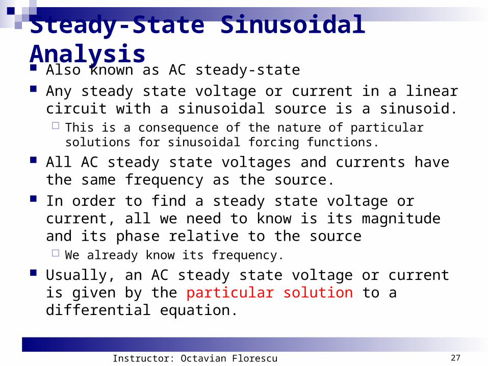
Steady-State Sinusoidal Analysis Also known as AC steady-state Any steady state voltage or current in a linear circuit with
a sinusoidal source is a sinusoid. This is a consequence of the nature of particular solutions for
sinusoidal forcing functions.
All AC steady state voltages and currents have the same frequency as the source.
In order to find a steady state voltage or current, all we need to know is its magnitude and its phase relative to the source We already know its frequency.
Usually, an AC steady state voltage or current is given by the particular solution to a differential equation.
EE40 Summer 2006: Lecture 5 Instructor: Octavian Florescu 28
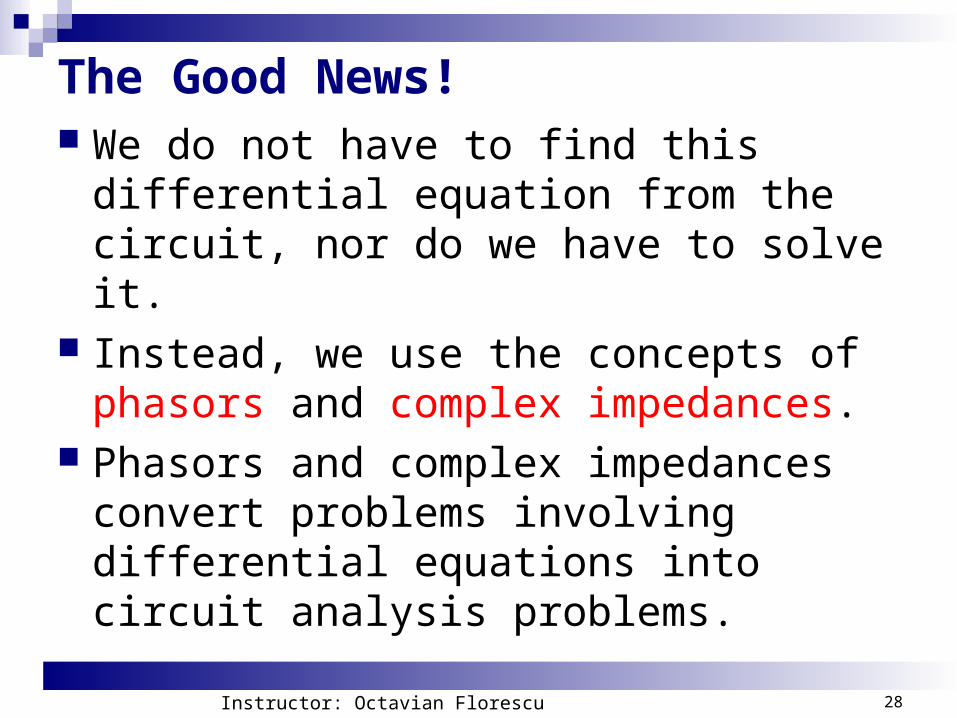
The Good News! We do not have to find this differential
equation from the circuit, nor do we have to solve it.
Instead, we use the concepts of phasors and complex impedances.
Phasors and complex impedances convert problems involving differential equations into circuit analysis problems.

EE40 Summer 2006: Lecture 5 Instructor: Octavian Florescu 29
Phasors A phasor is a complex number that
represents the magnitude and phase of a sinusoidal voltage or current.
Remember, for AC steady state analysis, this is all we need to compute-we already know the frequency of any voltage or current.

EE40 Summer 2006: Lecture 5 Instructor: Octavian Florescu 30
Complex Impedance Complex impedance describes the
relationship between the voltage across an element (expressed as a phasor) and the current through the element (expressed as a phasor).
Impedance is a complex number. Impedance depends on frequency. Phasors and complex impedance allow us
to use Ohm’s law with complex numbers to compute current from voltage and voltage from current.

EE40 Summer 2006: Lecture 5 Instructor: Octavian Florescu 31
Sinusoids
Amplitude: VM
Angular frequency: = 2 f Radians/sec
Phase angle: Frequency: f = 1/T
Unit: 1/sec or Hz Period: T
Time necessary to go through one cycle
( ) cosMv t V t

EE40 Summer 2006: Lecture 5 Instructor: Octavian Florescu 32
-8
-6
-4
2
4
6
8
-2
00 0.01 0.02 0.03 0.04 0.05
Phase
What is the amplitude, period, frequency, and radian frequency of this sinusoid?
EE40 Summer 2006: Lecture 5 Instructor: Octavian Florescu 33
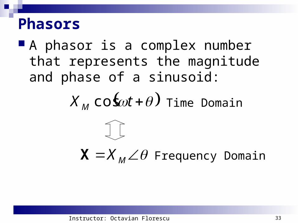
Phasors A phasor is a complex number that
represents the magnitude and phase of a sinusoid:
tX M cos
MXX
Time Domain
Frequency Domain