Embed Size (px)
Citation preview

EE462L, Power Electronics, Solar Power, I-V Characteristics Version January 31, 2012
Page 1 of 29
Report Details Choose any of the solar stations, but take your measurements only when the short circuit current is at least 3.5A. The weather forecast from www.weatherunderground.com can help you plan your schedule. Cloud cover forecast provided by the National Oceanic and Atmospheric Administration from http://www.nws.noaa.gov/forecasts/graphical/sectors/southplains.php#tabs can also be very helpful. For additional information and solar programs visit Dr. Grady’s web page at http://users.ece.utexas.edu/~grady Your report should include graphs of I versus V, and P versus V. Both actual data and Excel approximations should be plotted together. When plotting with Excel, be sure to use the “scatter plot” option so that the non-uniform spacing between voltage points on the x-axis show correctly. You should also work out numerical values for Equations (1) – (15) for the day and time of your measurements. Overview Incident sunlight can be converted into electricity by photovoltaic conversion using a solar panel. A solar panel consists of individual cells that are large-area semiconductor diodes, constructed so that light can penetrate into the region of the p-n junction. The junction formed between the n-type silicon wafer and the p-type surface layer governs the diode characteristics as well as the photovoltaic effect. Light is absorbed in the silicon, generating both excess holes and electrons. These excess charges can flow through an external circuit to produce power.
Figure 1. Equivalent Circuit of a Solar Cell
n-type
p-type
– V +
I
Photons
Junction
External circuit (e.g., battery,
lights)
Isc – V +
I
)1( BVeA
External circuit (e.g., battery,
lights)
0
5
0.0 0.6Diode Volts
Dio
de A
mp
s
EE462L, Power Electronics, Solar Power, I-V Characteristics Version January 31, 2012
Page 2 of 29
Diode current )1( BVeA comes from the standard I-V equation for a diode, plotted above. From Figure 1, it is clear that the current I that flows to the external circuit is
)1( BVsc eAII . If the solar cell is open circuited, then all of the scI flows through the
diode and produces an open circuit voltage of about 0.5-0.6V. If the solar cell is short circuited, then no current flows through the diode, and all of the scI flows through the short circuit.
Since the Voc for one cell is approximately 0.5-0.6V, then individual cells are connected in
series as a “solar panel” to produce more usable voltage and power output levels. Most solar panels are made to charge 12V batteries and consist of 36 individual cells (or units) in series to yield panel Voc ≈ 18-20V. The voltage for maximum panel power output is usually about 16-
17V. Each 0.5-0.6V series unit can contain a number of individual cells in parallel, thereby increasing the total panel surface area and power generating capability.
Figure 2. I-V Characteristics of Solar Panel On a clear day, direct normal solar insolation (i.e., incident solar energy) is approximately
2/1 mkW . Since solar panel efficiencies are approximately 14%, a solar panel will produce about 140W per square meter of surface area when facing a bright sun. High temperatures reduce panel efficiency. For 24/7 power availability, solar power must be stored in deep-discharge batteries that contain enough energy to power the load through the nighttime and overcast days. On good solar days in Austin, you can count on solar panels producing about 1kWH of energy per square meter. An everyday use of solar power is often seen in school zone and other LED flashing signs, where TxDOT and municipal governments find them economical when conventional electric service is not readily available or when the monthly minimum electric fees are large compared to the monthly kWH used. Look for solar panels on top of these signs, and also note their orientation.
V
I
Isc
Voc
Im
Vm
, where A, B, and especially Isc vary with solar insolation
0
0
Increasing solar insolation
mmIVP max
Maximum power point
)1( BVsc eAII

EE462L, Power Electronics, Solar Power, I-V Characteristics Version January 31, 2012
Page 3 of 29
The Solar Panels on ENS Rooftop The ENS rooftop is equipped with six pairs of commercial “12V class” panels, plus one larger “24V class” commercial panel. The panels are:
three pair of British Petroleum BP585, (mono-crystalline silicon, laser grooved, each panel 85W, voltage at maximum power = 18.0V, current at maximum power = 4.7A, open circuit voltage = 22.3V, short circuit current = 5.0A). These three pairs are connected to ENS212 stations 17, 18, and 19.
two pair of Solarex SX85U (now BP Solar) (polycrystalline silicon, each panel 85W, voltage at maximum power = 17.1V, current at maximum power = 5.0A, open circuit voltage = 21.3V, short circuit current = 5.3A). These two pairs are connected to ENS212 stations 15 and 16.
one pair of Photowatt PW750-80 (multi-crystalline cells, each panel 80W, voltage at maximum power = 17.3V, current at maximum power = 4.6A, open circuit voltage = 21.9V, short circuit current = 5.0A). This pair is connected to ENS212 station 21.
one British Petroleum BP3150U, 150W panel (multicrystalline), open circuit voltage = 43.5V, short circuit current = 4.5A. This is connected to ENS212 station 20.
Each of the seven stations is wired to ENS212 and has an open circuit voltage of approximately 40V and a short circuit current of approximately 5A. The I-V and P-V characteristics for one of the panel pairs is shown in Figure 3. The I-V curve fit equation for Figure 3 is
100524.034.5)( 1777.0 VeVI .

EE462L, Power Electronics, Solar Power, I-V Characteristics Version January 31, 2012
Page 4 of 29
Maximum Power As seen in bottom figure of Figure 3, panels have a maximum power point. Maximum power corresponds to Vm and Im in Figure 2. Because solar power is relatively expensive (approx. $4-
5 per watt for the panels, plus the same amount for batteries and electronics), it is important to operate panels at their maximum power conditions. Unfortunately, Vm, Im, and the Thevenin
PV Station 13, Bright Sun, Dec. 6, 2002
0
1
2
3
4
5
6
0 5 10 15 20 25 30 35 40 45
V(panel) - volts
I - a
mp
s
PV Station, Bright Sun
PV Station 13, Bright Sun, Dec. 6, 2002
0.0
20.0
40.0
60.0
80.0
100.0
120.0
140.0
0 5 10 15 20 25 30 35 40 45
V(panel) - volts
P(p
an
el)
- w
att
s
PV Station, Bright Sun
Figure 3. I-V and P-V Characteristics for One of the Panel Pairs (data points taken by loading the panel pair with a variable load resistor)
EE462L, Power Electronics, Solar Power, I-V Characteristics Version January 31, 2012
Page 5 of 29
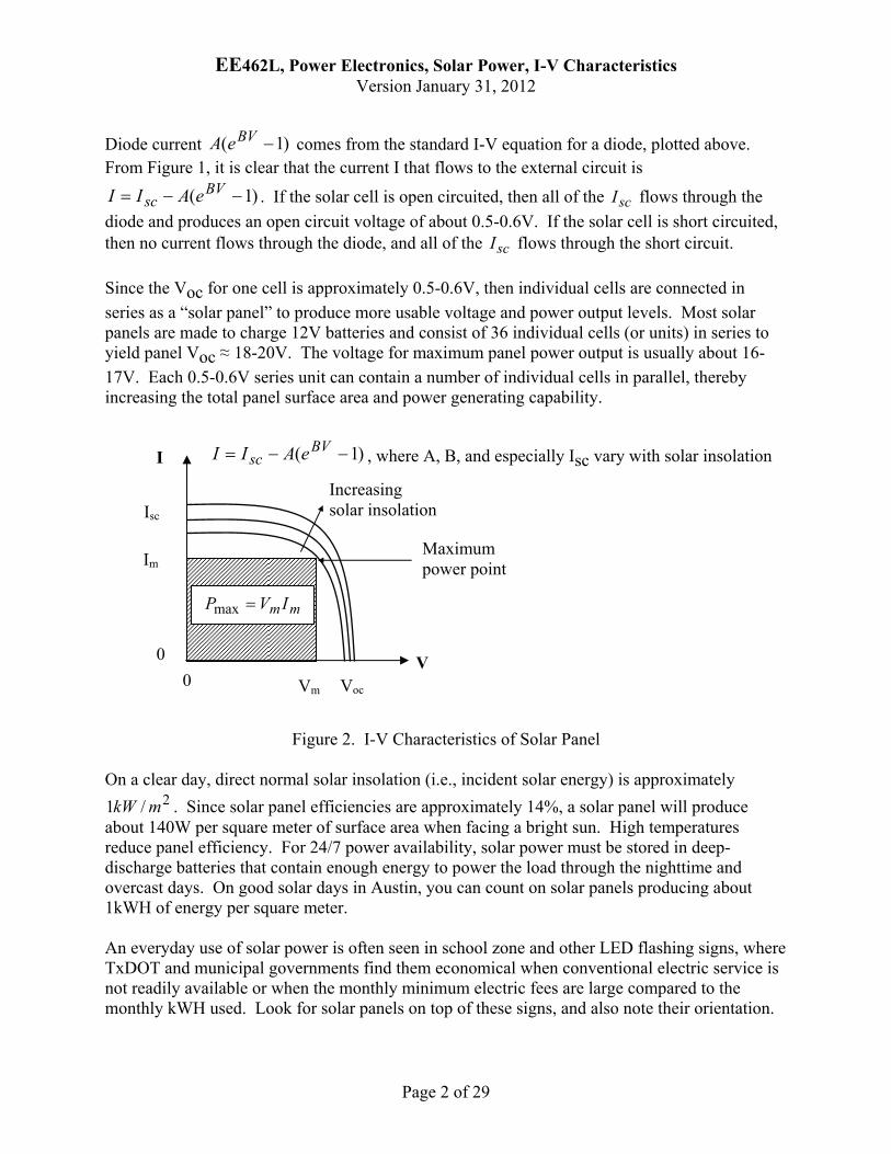
equivalent resistance vary with light level. DC-DC converters are often used to “match” the load resistance to the Thevenin equivalent resistance of the panel to maximize the power drawn from the panel. These “smart” converters (often referred to as “tracking converters”) also charge the storage batteries in such a way as to maximize battery life. Sun Position Ideally, a solar panel should track the sun so that the incident solar rays are perpendicular to the panel surface, thus maximizing the capture of solar energy. However, because of high wind loads, most panels are fixed in position. Often, panel tilt (with respect to horizontal) is adjusted seasonally. Orientation of fixed panels should be carefully chosen to capture the most energy for the year, or for a season. The position of the sun in the sky varies dramatically with hour and season. Sun zenith angle
zenithsun is expressed in degrees from vertical. Sun azimuth azimuth
sun is expressed in degrees
from true north. Sun zenith and azimuth angles are illustrated in Figure 4. Sun position angles are available in many references, and with different levels of complexity. For our purposes, we use the following equations (1) – (7) taken from the University of Oregon Solar Radiation Monitoring Laboratory (http://solardat.uoregon.edu/SolarRadiationBasics.html):
Sun declination angle (in radians) is
365
2842sin
18045.23
n , n = day of year (i.e., 1,2,3, … , 364,365). (1)
Equation of time (in decimal minutes) is
Figure 4. Sun Zenith and Azimuth Angles
West
North (x axis)
Line perpendicular to horizontal plane
East (y axis)
Horizontal plane
Up (−z axis)
zenithsun
azimuthsun
Note – because of magnetic declination, a compass in Austin points approximately 6º east of north.

EE462L, Power Electronics, Solar Power, I-V Characteristics Version January 31, 2012
Page 6 of 29
for
111
)7(sin2.14 ,1061
nEn qt ,
for
59
)106(sin0.4 ,166107
nEn qt ,
for
80
)166(sin5.6 ,246167
nEn qt ,
for
113
)247(sin4.16 ,365247
nEn qt . (2)
Solar time (in decimal hours) is
1560
localtimezoneqtlocalsolar
LongitudeLongitudeETT
, (3)
where
localT is local standard time in decimal hours,
timezoneLongitude is the longitude at the eastern edge of the time zone (e.g., 90 for
Central Standard Time). (Note – in the Solar_Data_Analyzer program, localtimezone LongitudeLongitude is
entered as “Longitude shift (deg).” At Austin, with 74.97localLongitude , the
longitude shift is 74.774.9790 . The latitude at Austin is 30.29°.). Hour angle (in radians) is
12
12 solarT . (4)
Cosine of the zenith angle is
)cos()cos()cos()sin()sin(cos zenithsun , (5)
where is the latitude of the location.
Solar azimuth comes from the following calculations. Using the formulas for solar radiation on tilted surfaces, consider vertical surfaces directed east and south. The fraction of direct component of solar radiation on an east-facing vertical surface is
EE462L, Power Electronics, Solar Power, I-V Characteristics Version January 31, 2012
Page 7 of 29
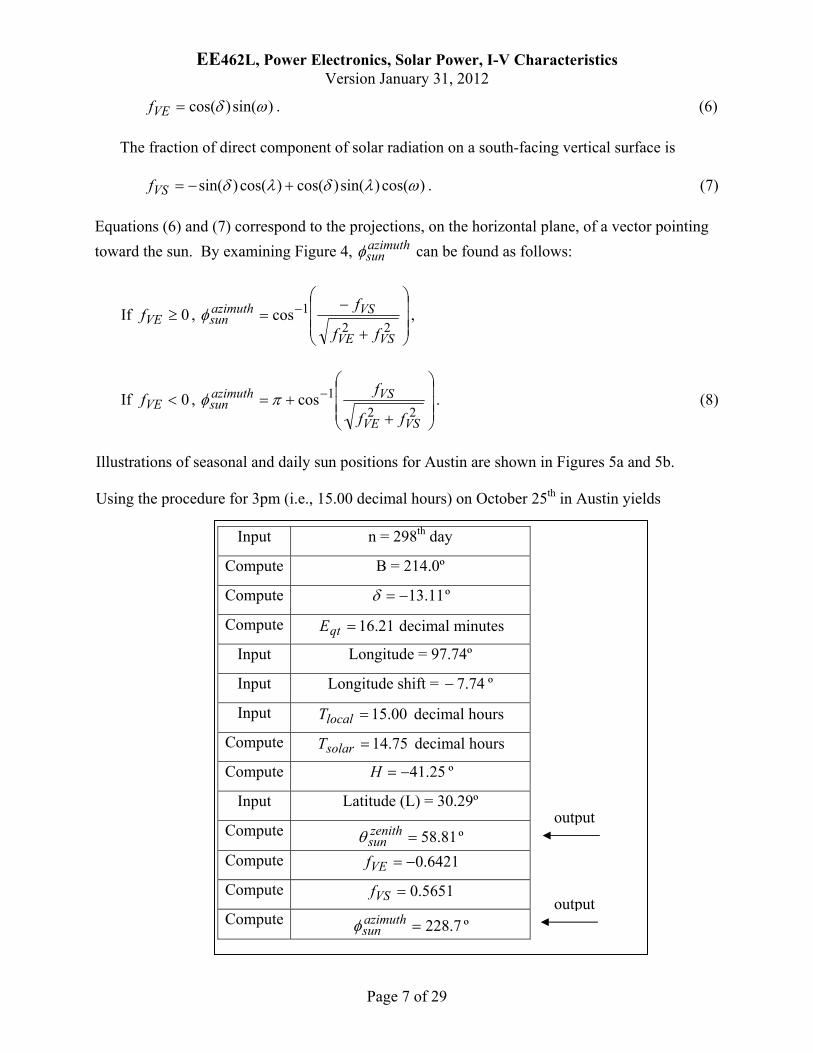
)sin()cos( VEf . (6)
The fraction of direct component of solar radiation on a south-facing vertical surface is
)cos()sin()cos()cos()sin( VSf . (7)
Equations (6) and (7) correspond to the projections, on the horizontal plane, of a vector pointing
toward the sun. By examining Figure 4, azimuthsun can be found as follows:
If 0VEf ,
22
1cos
VSVE
VSazimuthsun
ff
f ,
If 0VEf ,
22
1cos
VSVE
VSazimuthsun
ff
f . (8)
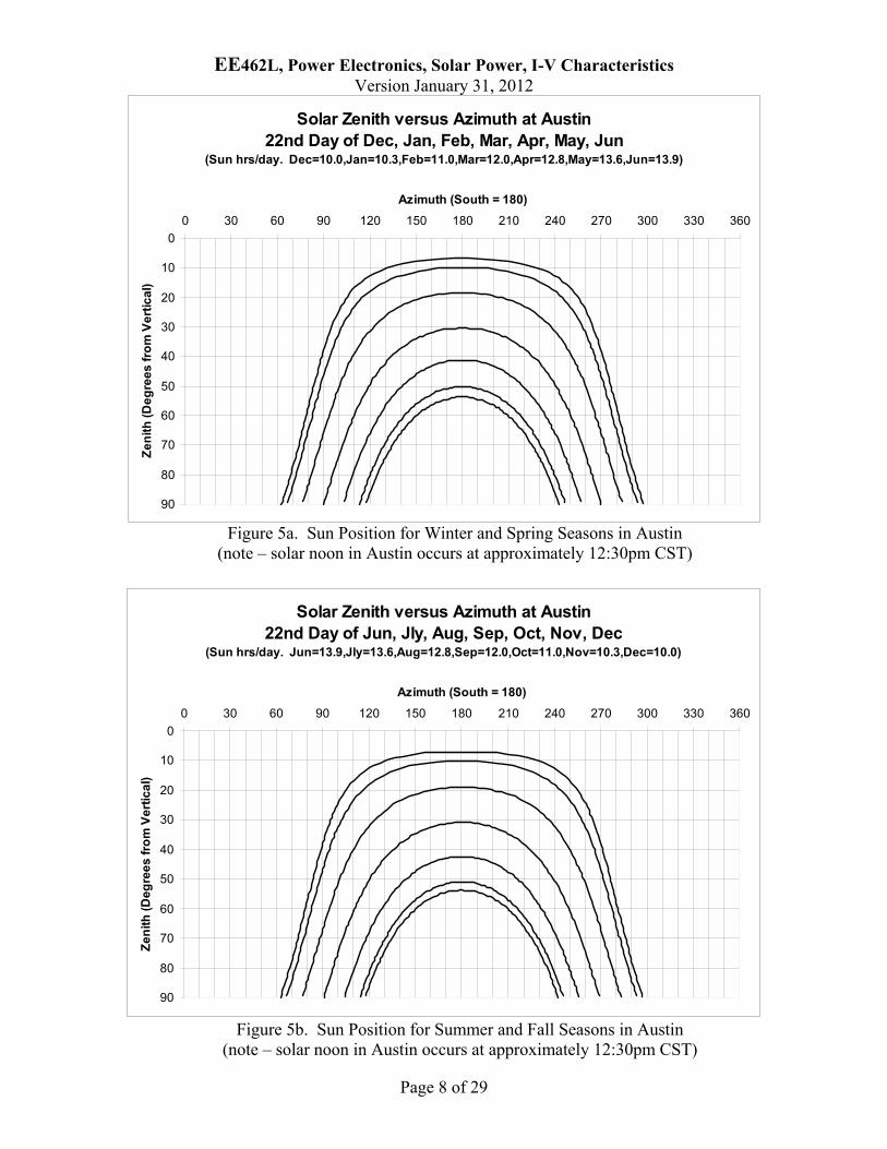
Illustrations of seasonal and daily sun positions for Austin are shown in Figures 5a and 5b. Using the procedure for 3pm (i.e., 15.00 decimal hours) on October 25th in Austin yields
Input n = 298th day
Compute B = 214.0º
Compute 11.13 º
Compute 21.16qtE decimal minutes
Input Longitude = 97.74º
Input Longitude shift = 74.7 º
Input 00.15localT decimal hours
Compute 75.14solarT decimal hours
Compute 25.41H º
Input Latitude (L) = 30.29º
Compute 81.58zenithsun º
Compute 6421.0VEf
Compute 5651.0VSf
Compute 7.228azimuthsun º
output
output
EE462L, Power Electronics, Solar Power, I-V Characteristics Version January 31, 2012
Page 8 of 29
Figure 5a. Sun Position for Winter and Spring Seasons in Austin (note – solar noon in Austin occurs at approximately 12:30pm CST)
Figure 5b. Sun Position for Summer and Fall Seasons in Austin (note – solar noon in Austin occurs at approximately 12:30pm CST)
Solar Zenith versus Azimuth at Austin22nd Day of Dec, Jan, Feb, Mar, Apr, May, Jun
(Sun hrs/day. Dec=10.0,Jan=10.3,Feb=11.0,Mar=12.0,Apr=12.8,May=13.6,Jun=13.9)
0
10
20
30
40
50
60
70
80
90
0 30 60 90 120 150 180 210 240 270 300 330 360
Azimuth (South = 180)
Ze
nit
h (
De
gre
es f
rom
Ver
tic
al)
Solar Zenith versus Azimuth at Austin22nd Day of Jun, Jly, Aug, Sep, Oct, Nov, Dec
(Sun hrs/day. Jun=13.9,Jly=13.6,Aug=12.8,Sep=12.0,Oct=11.0,Nov=10.3,Dec=10.0)
0
10
20
30
40
50
60
70
80
90
0 30 60 90 120 150 180 210 240 270 300 330 360
Azimuth (South = 180)
Ze
nit
h (
Deg
ree
s f
rom
Ve
rtic
al)

EE462L, Power Electronics, Solar Power, I-V Characteristics Version January 31, 2012
Page 9 of 29
Definitions from www.weatherground.com
Twilight This is the time before sunrise and after sunset where it is still light outside, but the sun is not in the sky.
Civil Twilight This is defined to be the time period when the sun is no more than 6 degrees below the horizon at either sunrise or sunset. The horizon should be clearly defined and the brightest stars should be visible under good atmospheric conditions (i.e. no moonlight, or other lights). One still should be able to carry on ordinary outdoor activities.
Nautical Twilight
This is defined to be the time period when the sun is between 6 and 12 degrees below the horizon at either sunrise or sunset. The horizon is not defined and the outline of objects might be visible without artificial light. Ordinary outdoor activities are not possible at this time without extra illumination.
Astronomical Twilight
This is defined to be the time period when the sun is between 12 and 18 degrees below the horizon at either sunrise or sunset. The sun does not contribute to the illumination of the sky before this time in the morning, or after this time in the evening. In the beginning of morning astronomical twilight and at the end of astronomical twilight in the evening, sky illumination is very faint, and might be undetectable.
Length Of Day This is defined to be the time of Actual Sunset minus the time of Actual Sunrise. The change in length of daylight between today and tomorrow is also listed when available.
Length Of Visible Light
This is defined to be the time of Civil Sunset minus the time of Civil Sunrise.
Altitude (or Elevation)
First, find your azimuth. Next, the Altitude (or elevation) is the angle between the Earth's surface (horizon) and the sun, or object in the sky. Altitudes range from -90° (straight down below the horizon, or the nadir) to +90° (straight up above the horizon or the Zenith) and 0° straight at the horizon.
Azimuth The azimuth (az) angle is the compass bearing, relative to true (geographic) north, of a point on the horizon directly beneath the sun. The horizon is defined as an imaginary circle centered on the observer. This is the 2-D, or Earth's surface, part of calculating the sun's position. As seen from above the observer, these compass bearings are measured clockwise in degrees from north. Azimuth angles can range from 0 - 359°. 0° is due geographic north, 90° due east, 180° due south, and 360 due north again.

EE462L, Power Electronics, Solar Power, I-V Characteristics Version January 31, 2012
Page 10 of 29
Hour Angle of the Sun
The Solar Hour Angle of the Sun for any local location on the Earth is zero° when the sun is straight overhead, at the zenith, and negative before local solar noon and positive after solar noon. In one 24-hour period, the Solar Hour Angle changes by 360 degrees (i.e. one revolution).
Mean Anomaly of the Sun
The movement of the Earth around the Sun is an ellipse. However, if the movement of the Earth around the Sun were a circle, it would be easy to calculate its position. Since, the Earth moves around the sun about one degree per day, (in fact, it's 1/365.25 of the circle), we say the Mean Anomaly of the Sun is the position of the Earth along this circular path. The True Anomaly of the Sun is the position along its real elliptical path.
Obliquity Obliquity is the angle between a planet's equatorial plane and its orbital plane.
Right Ascension of the Sun
The Celestial Sphere is a sphere where we project objects in the sky. We project stars, the moon, and sun, on to this imaginary sphere. The Right Ascension of the Sun is the position of the sun on our Celestial Sphere
Solar Noon (and Solar Time)
Solar Time is based on the motion of the sun around the Earth. The apparent sun's motion, and position in the sky, can vary due to a few things such as: the elliptical orbits of the Earth and Sun, the inclination of the axis of the Earth's rotation, the perturbations of the moon and other planets, and of course, your latitude and longitude of observation. Solar Noon is when the sun is at the highest in the sky, and is defined when the Hour Angle is 0°. Solar Noon is also the midpoint between Sunrise and Sunset.
Sun Declination
The Declination of the sun is how many degrees North (positive) or South (negative) of the equator that the sun is when viewed from the center of the earth. The range of the declination of the sun ranges from approximately +23.5° (North) in June to -23.5° (South) in December.
EE462L, Power Electronics, Solar Power, I-V Characteristics Version January 31, 2012
Page 11 of 29
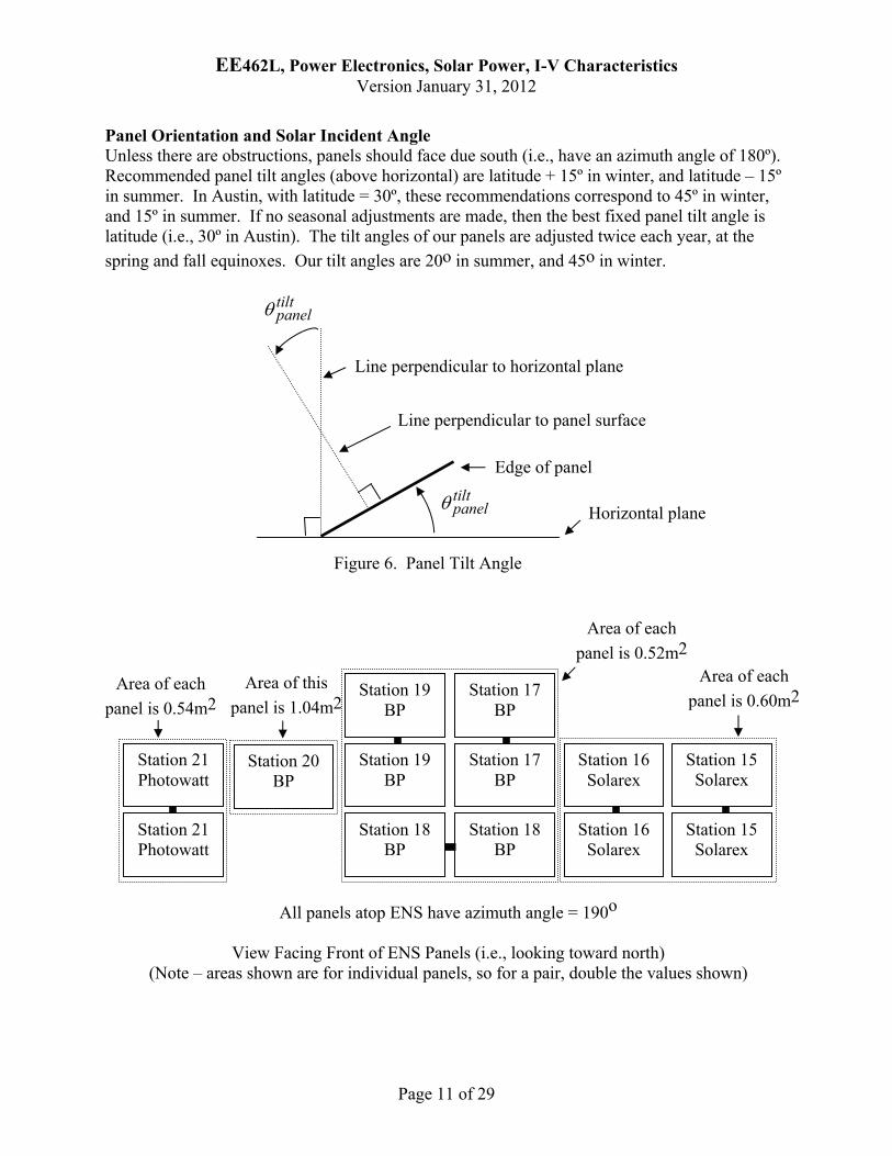
Panel Orientation and Solar Incident Angle Unless there are obstructions, panels should face due south (i.e., have an azimuth angle of 180º). Recommended panel tilt angles (above horizontal) are latitude + 15º in winter, and latitude – 15º in summer. In Austin, with latitude = 30º, these recommendations correspond to 45º in winter, and 15º in summer. If no seasonal adjustments are made, then the best fixed panel tilt angle is latitude (i.e., 30º in Austin). The tilt angles of our panels are adjusted twice each year, at the
spring and fall equinoxes. Our tilt angles are 20o in summer, and 45o in winter.
tiltpanel
Line perpendicular to horizontal plane
tiltpanel
Horizontal plane
Figure 6. Panel Tilt Angle
Line perpendicular to panel surface
Edge of panel
All panels atop ENS have azimuth angle = 190o
View Facing Front of ENS Panels (i.e., looking toward north) (Note – areas shown are for individual panels, so for a pair, double the values shown)
Station 18 BP
Station 19 BP
Station 18 BP
Station 17 BP
Station 16 Solarex
Station 16 Solarex
Station 19 BP
Station 17 BP
Station 15 Solarex
Station 15 Solarex
Station 21 Photowatt
Station 21 Photowatt
Area of each
panel is 0.54m2
Area of each
panel is 0.52m2 Area of each
panel is 0.60m2
Station 20 BP
Area of this
panel is 1.04m2
EE462L, Power Electronics, Solar Power, I-V Characteristics Version January 31, 2012
Page 12 of 29
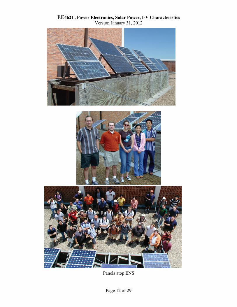
Panels atop ENS

EE462L, Power Electronics, Solar Power, I-V Characteristics Version January 31, 2012
Page 13 of 29
The angle between the rays of the sun and a vector perpendicular to the panel surface is known as the angle of incidence ( incident ). The cosine of incident is found by first expressing a unit
vector pointed toward the sun, and a unit vector perpendicular to the panel surface, and then taking the dot product of the two unit vectors. When 1)cos( incident , then the sun’s rays are
perpendicular to the panel surface, so that maximum incident solar energy is captured. The expressions follow. Considering Figure 4, the unit vector pointed toward the sun is
zyxsun aaaa ˆcosˆsinsinˆcossinˆ zenithsun
azimuthsun
zenithsun
azimuthsun
zenithsun .
Considering Figure 6, the unit vector perpendicular to the panel surface is
zyxpanel aaaa ˆcosˆsinsinˆcossinˆ tiltpanel
azimuthpanel
tiltpanel
azimuthpanel
tiltpanel
The dot product of the two unit vectors is then
azimuthpanel
tiltpanel
azimuthsun
zenithsunincident cossincossinˆˆcos panelsun aa
azimuthpanel
tiltpanel
azimuthsun
zenithsun sinsinsinsin tilt
panelzenithsun coscos .
Combining terms yields
azimuthpanel
azimuthsun
azimuthpanel
azimuthsun
tiltpanel
zenithsunincident sinsincoscossinsincos
tiltpanel
zenithsun coscos .
Simplifying the above equation yields the general case,
tiltpanel
zenithsun
azimuthpanel
azimuthsun
tiltpanel
zenithsunincident coscoscossinsincos . (9)
Some special cases are
1. Flat panel (i.e., 0tiltpanel ). Then,
zenithsunincident coscos .
EE462L, Power Electronics, Solar Power, I-V Characteristics Version January 31, 2012
Page 14 of 29
2. Sun directly overhead (i.e., 0sunzenith ). Then,
tiltpanelincident coscos .
3. Equal azimuth angles (i.e., azimuth tracking, azimuthpanel
azimuthsun ). Then,
tiltpanel
zenithsun
tiltpanel
zenithsun
tiltpanel
zenithsunincident coscoscossinsincos .
4. Sun zenith angle equals panel tilt angle (i.e., zenith tracking, tiltpanel
zenithsun ). Then,
zenithsun
azimuthpanel
azimuthsun
zenithsunincident 22 coscossincos .
To illustrate the general case, consider the following example: 3pm (standard time) in Austin on October 25. The sun position is
azimuthsun = 228.7º, zenith
sun = 58.8º, so that zyxsun aaaa ˆ517.0ˆ643.0ˆ565.0ˆ ,
and the panel angles are
azimuthpanel = 190º, tilt
panel = 45º, so that zyxpanel aaaa ˆ707.0ˆ1228.0ˆ696.0ˆ .
Evaluating the dot product yields incidentcos = 0.838, so incident = 33.1º.
Solar Radiation Measurements The three most important solar radiation measurements for studying solar panel performance are global horizontal (GH), diffuse horizontal (DH), and direct normal (DN). GH is “entire sky,” including the sun disk, looking straight up. DH is “entire sky,” excluding the sun disk, looking
straight up. DN is facing directly toward the sun. The units for GH, DH, and DN are W/m2. The direct measurement of DN requires a sun tracking device. The Sci Tek 2AP tracker takes DN, GH, and DH readings every five minutes using three separate thermocouple sensors. The DN sensor tracks and sees only the disk of the sun. The GH sensor points straight up and sees the entire sky with sun disk. The DH sensor points straight up, but a shadow ball blocks the disk of the sun, so that it sees entire sky minus sun disk. Rotating shadowband pyranometers use one PV sensor, pointed straight up, to measure GH and DH every minute, and then save average values every 5 minutes. Once per minute, the shadow band swings over, and when the shadow falls on the sensor, the DH reading is taken. Using GH and DH, the rotating shadow-band pyranometer estimates DN.
EE462L, Power Electronics, Solar Power, I-V Characteristics Version January 31, 2012
Page 15 of 29
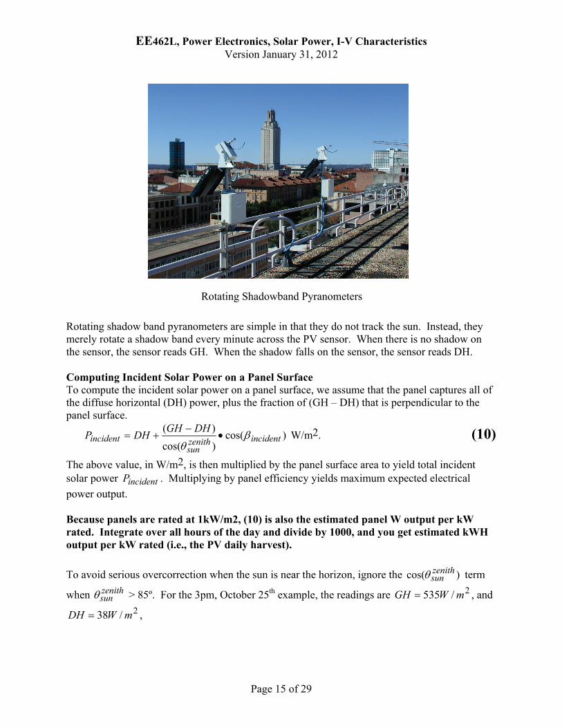
Rotating shadow band pyranometers are simple in that they do not track the sun. Instead, they merely rotate a shadow band every minute across the PV sensor. When there is no shadow on the sensor, the sensor reads GH. When the shadow falls on the sensor, the sensor reads DH. Computing Incident Solar Power on a Panel Surface To compute the incident solar power on a panel surface, we assume that the panel captures all of the diffuse horizontal (DH) power, plus the fraction of (GH – DH) that is perpendicular to the panel surface.
)cos()cos(
)(incidentzenith
sunincident
DHGHDHP
W/m2. (10)
The above value, in W/m2, is then multiplied by the panel surface area to yield total incident solar power incidentP . Multiplying by panel efficiency yields maximum expected electrical
power output. Because panels are rated at 1kW/m2, (10) is also the estimated panel W output per kW rated. Integrate over all hours of the day and divide by 1000, and you get estimated kWH output per kW rated (i.e., the PV daily harvest).
To avoid serious overcorrection when the sun is near the horizon, ignore the )cos( zenithsun term
when zenithsun > 85º. For the 3pm, October 25th example, the readings are 2/535 mWGH , and
2/38 mWDH ,
Rotating Shadowband Pyranometers

EE462L, Power Electronics, Solar Power, I-V Characteristics Version January 31, 2012
Page 16 of 29
panelincident AP
)1.33cos()9.58cos(
)38535(38 = 2/ 844 mWApanel ,
which means that a PV panel or array would produce 844 W per kW rated power.
NREL Sci Tec Two-Axis Tracker
EE462L, Power Electronics, Solar Power, I-V Characteristics Version January 31, 2012
Page 17 of 29
The Experiment Your assignment is to measure the I-V and P-V characteristics of a solar panel pair, plot the points, determine maximum power, estimate panel efficiency, and use the Excel Solver to approximate the I-V and P-V curves using
)1( BVsc eAII , )1( BV
sc eAIVVIP ,
where the Solver estimates coefficients Isc, A, and B from your measured I-V data set. See the
Appendix for a description of the Excel Solver.
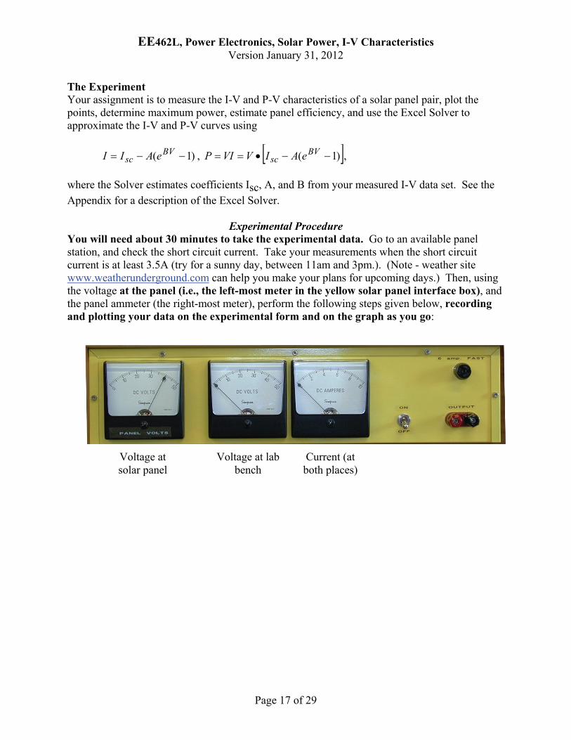
Experimental Procedure You will need about 30 minutes to take the experimental data. Go to an available panel station, and check the short circuit current. Take your measurements when the short circuit current is at least 3.5A (try for a sunny day, between 11am and 3pm.). (Note - weather site www.weatherunderground.com can help you make your plans for upcoming days.) Then, using the voltage at the panel (i.e., the left-most meter in the yellow solar panel interface box), and the panel ammeter (the right-most meter), perform the following steps given below, recording and plotting your data on the experimental form and on the graph as you go:
Voltage at solar panel
Voltage at lab bench
Current (at both places)

EE462L, Power Electronics, Solar Power, I-V Characteristics Version January 31, 2012
Page 18 of 29
Form and Graph for Recording and Plotting Your Readings as You Take Them (have this page signed by Dr. Kwasinski or one of the TAs before beginning your report)
Panel Station = ____ Date and Time of Measurements= ___________, Sky Conditions = _____
Vpanel* Ipanel* P (i.e., Vpanel
● Ipanel )
Notes
Voc = Open circuit condition
Isc = Short Circuit Condition
* Vpanel (i.e., at the panel) is the left-most meter in the yellow interface box, and Ipanel is the
right-most meter.
0V 10V 20V 30V 40V 50V
6A
5A
4A
3A
2A
1A
0A
≈2V spacing for V > 25V
≈5V spacing for V ≤ 25V
EE462L, Power Electronics, Solar Power, I-V Characteristics Version January 31, 2012
Page 19 of 29
Steps
1. Measure the panel pair’s open circuit voltage, and record in the table and on the graph. The current is zero for this case.
2. Short the output terminals with one of the red shorting bar or with a wire. Measure the short circuit current and panel pair voltage. Record both and add the point to your graph. The panel voltage will be small for this condition.
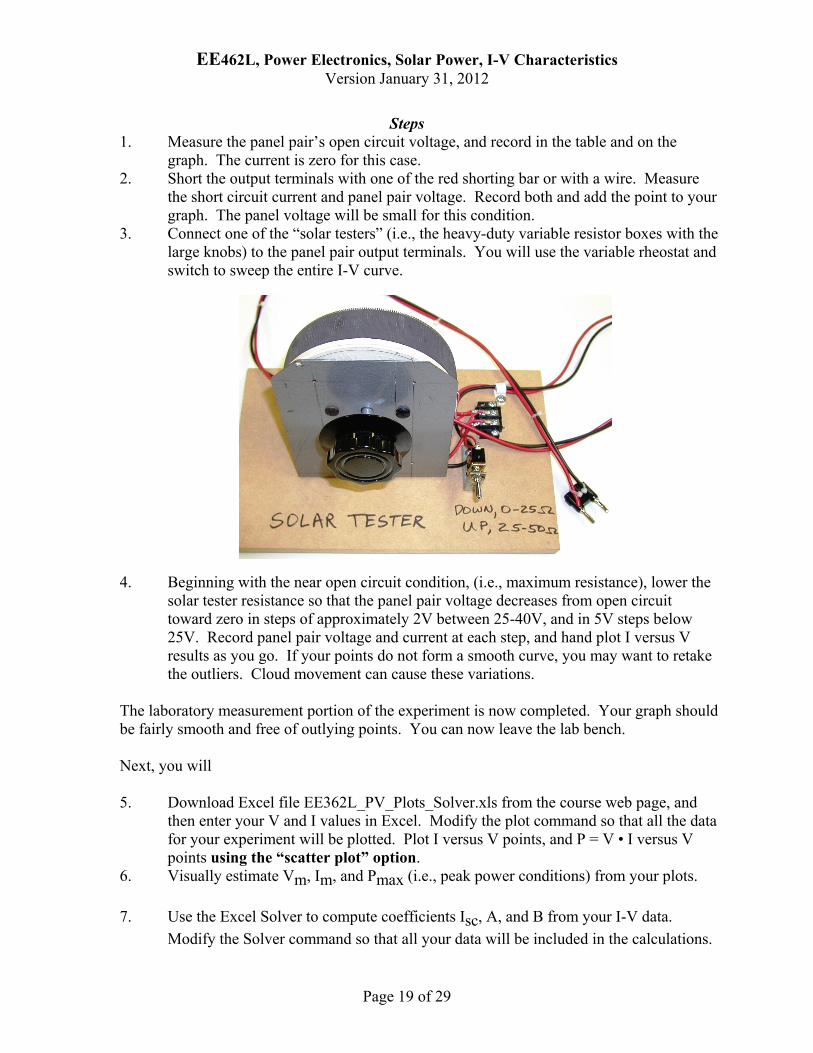
3. Connect one of the “solar testers” (i.e., the heavy-duty variable resistor boxes with the large knobs) to the panel pair output terminals. You will use the variable rheostat and switch to sweep the entire I-V curve.
4. Beginning with the near open circuit condition, (i.e., maximum resistance), lower the
solar tester resistance so that the panel pair voltage decreases from open circuit toward zero in steps of approximately 2V between 25-40V, and in 5V steps below 25V. Record panel pair voltage and current at each step, and hand plot I versus V results as you go. If your points do not form a smooth curve, you may want to retake the outliers. Cloud movement can cause these variations.
The laboratory measurement portion of the experiment is now completed. Your graph should be fairly smooth and free of outlying points. You can now leave the lab bench. Next, you will 5. Download Excel file EE362L_PV_Plots_Solver.xls from the course web page, and
then enter your V and I values in Excel. Modify the plot command so that all the data for your experiment will be plotted. Plot I versus V points, and P = V • I versus V points using the “scatter plot” option.
6. Visually estimate Vm, Im, and Pmax (i.e., peak power conditions) from your plots.
7. Use the Excel Solver to compute coefficients Isc, A, and B from your I-V data.
Modify the Solver command so that all your data will be included in the calculations.

EE462L, Power Electronics, Solar Power, I-V Characteristics Version January 31, 2012
Page 20 of 29
Superimpose the Solver equations on the I-V and P-V graphs of Step 5. See the Appendix for Solver instructions. Use your Solver graph to estimate Pmax.
Now, use the following steps to estimate panel pair efficiency: 8. Go to the class web page and download the Excel spreadsheet and solar data file
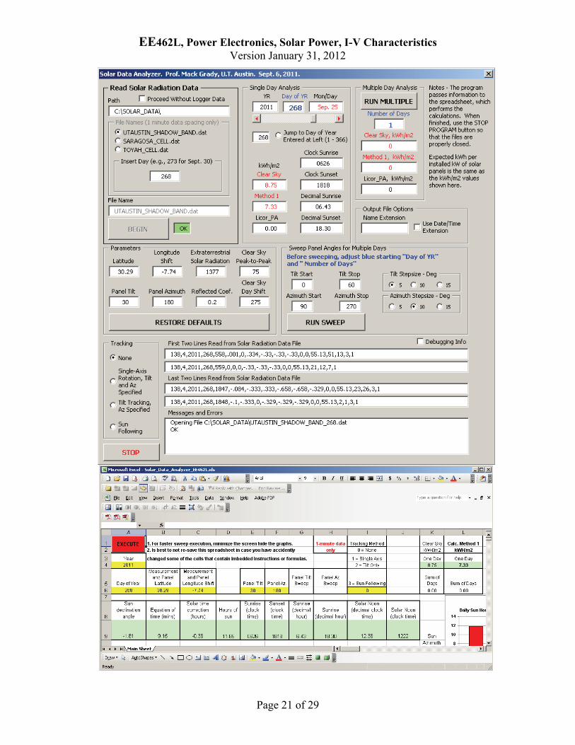
Solar_Data_Analyzer_EE462L.xls, and SOLAR_DATA_through_XXX.zip, (XXX is the last data day in the zip) Note – the 1-minute data averages are recorded by a shadow band tracker atop ETC and are updated daily on the web page while EE462L is being taught. Due to equipment malfunction please refer to the attached file called solar instructions.pdf for information about how to proceed in this step.
9. Display the data for your day (note – these data are given in Central Standard Time). 10. For the minute that best represents your time of measurements, work through the Big 10
equations. 11. Compare your Big 10 equations to the Solar_Data_Analyzer spreadsheet values for your
day/minute. 12. For your day, use the Solar_Data_Analyzer spreadsheet as indicated in the solar
instructions.pdf file to predict Method 1 daily kWh per installed kW for fixed panel azimuth = 180, and panel tilts 20, 30, and 40 degrees, for single axis tracking, azimuth = 180, tilt = 20 and 30, for two-axis tracking.
Interpret and comment on the results.
EE462L, Power Electronics, Solar Power, I-V Characteristics Version January 31, 2012
Page 21 of 29
EE462L, Power Electronics, Solar Power, I-V Characteristics Version January 31, 2012
Page 22 of 29
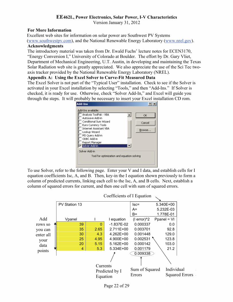
For More Information Excellent web sites for information on solar power are Southwest PV Systems (www.southwestpv.com), and the National Renewable Energy Laboratory (www.nrel.gov). Acknowledgments The introductory material was taken from Dr. Ewald Fuchs’ lecture notes for ECEN3170, “Energy Conversion I,” University of Colorado at Boulder. The effort by Dr. Gary Vliet, Department of Mechanical Engineering, U.T. Austin, in developing and maintaining the Texas Solar Radiation web site is greatly appreciated. We also appreciate the use of the Sci Tec two-axis tracker provided by the National Renewable Energy Laboratory (NREL). Appendix A: Using the Excel Solver to Curve-Fit Measured Data The Excel Solver is not part of the “Typical User” installation. Check to see if the Solver is activated in your Excel installation by selecting “Tools,” and then “Add-Ins.” If Solver is checked, it is ready for use. Otherwise, check “Solver Add-In,” and Excel will guide you through the steps. It will probably be necessary to insert your Excel installation CD rom.
To use Solver, refer to the following page. Enter your V and I data, and establish cells for I equation coefficients Isc, A, and B. Then, key-in the I equation shown previously to form a column of predicted currents, linking each cell to the Isc, A, and B cells. Next, establish a column of squared errors for current, and then one cell with sum of squared errors.
PV Station 13 Isc= 5.340E+00 A= 5.232E-03 B= 1.778E-01
Vpanel I I equation (I error)^2 Ppanel = VI 39 0 -1.837E-02 0.000337 0.0 35 2.65 2.711E+00 0.003701 92.8 30 4.3 4.262E+00 0.001448 129.0 25 4.95 4.900E+00 0.002531 123.8 20 5.15 5.162E+00 0.000142 103.0
4 5.3 5.334E+00 0.001179 21.2 0.009338
Coefficients of I Equation
Currents Predicted by I Equation
Sum of Squared Errors
Individual Squared Errors
Add rows so you can enter all
your data
points

EE462L, Power Electronics, Solar Power, I-V Characteristics Version January 31, 2012
Page 23 of 29
Now, under “Tools,” select “Solver.” The following window will appear. Enter your “Target Cell” (the sum of squared errors cell), plus the “Changing Cells” that correspond to Isc, A, and B. It is for your starting values for Isc, A, and B are reasonable. You should probably use
the A and B values shown above as your starting point. Use your own measured short circuit current for Isc.
Be sure to request “Min” to minimize the error, and then click “Solve.”
If successful, click “OK” and then plot your measured I, and your estimated I, versus V to make a visual comparison between the measured and estimated currents. Use the scatter plot option to maintain proper spacing between voltage points on the x-axis. If unsuccessful when curve fitting, try changing Isc, A, or B, and re-try.
EE462L, Power Electronics, Solar Power, I-V Characteristics Version January 31, 2012
Page 24 of 29
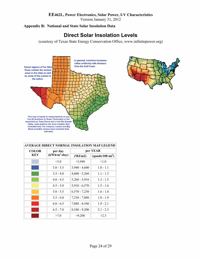
Appendix B: National and State Solar Insolation Data
Direct Solar Insolation Levels (courtesy of Texas State Energy Conservation Office, www.infinitepower.org)
AVERAGE DIRECT NORMAL INSOLATION MAP LEGEND
per YEAR COLOR KEY
per day (kWh/m2-day) (MJ/m2) (quads/100 mi2)
<3.0 <3,940 <1.0
3.0 - 3.5 3,940 - 4,600 1.0 - 1.1
3.5 - 4.0 4,600 - 5,260 1.1 - 1.3
4.0 - 4.5 5,260 - 5,910 1.3 - 1.5
4.5 - 5.0 5,910 - 6,570 1.5 - 1.6
5.0 - 5.5 6,570 - 7,230 1.6 - 1.8
5.5 - 6.0 7,230 - 7,880 1.8 - 1.9
6.0 - 6.5 7,880 - 8,540 1.9 - 2.1
6.5 - 7.0 8,540 - 9,200 2.1 - 2.3
>7.0 >9,200 >2.3
EE
462L
, Pow
er E
lect
ron
ics,
Sol
ar P
ower
, I-V
Ch
arac
teri
stic
s V
ersi
on J
anua
ry 3
1, 2
012
Pag
e 25
of
29
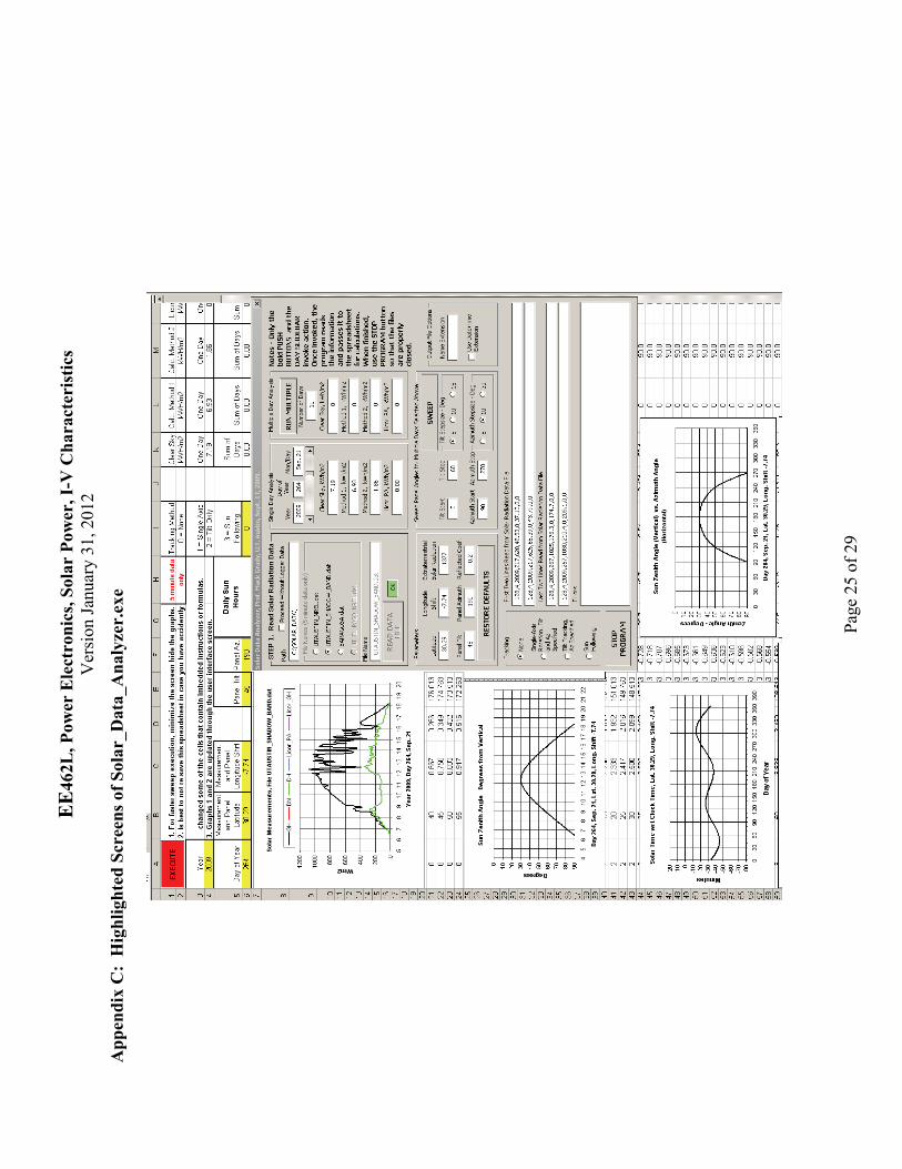
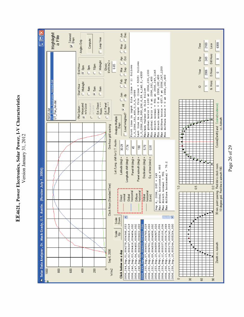
Ap
pen
dix
C:
Hig
hli
ghte
d S
cree
ns o
f S
olar
_Dat
a_A
nal
yzer
.exe
EE
462L
, Pow
er E
lect
ron
ics,
Sol
ar P
ower
, I-V
Ch
arac
teri
stic
s V
ersi
on J
anua
ry 3
1, 2
012
Pag
e 26
of
29
EE
462L
, Pow
er E
lect
ron
ics,
Sol
ar P
ower
, I-V
Ch
arac
teri
stic
s V
ersi
on J
anua
ry 3
1, 2
012
Pag
e 27
of
29
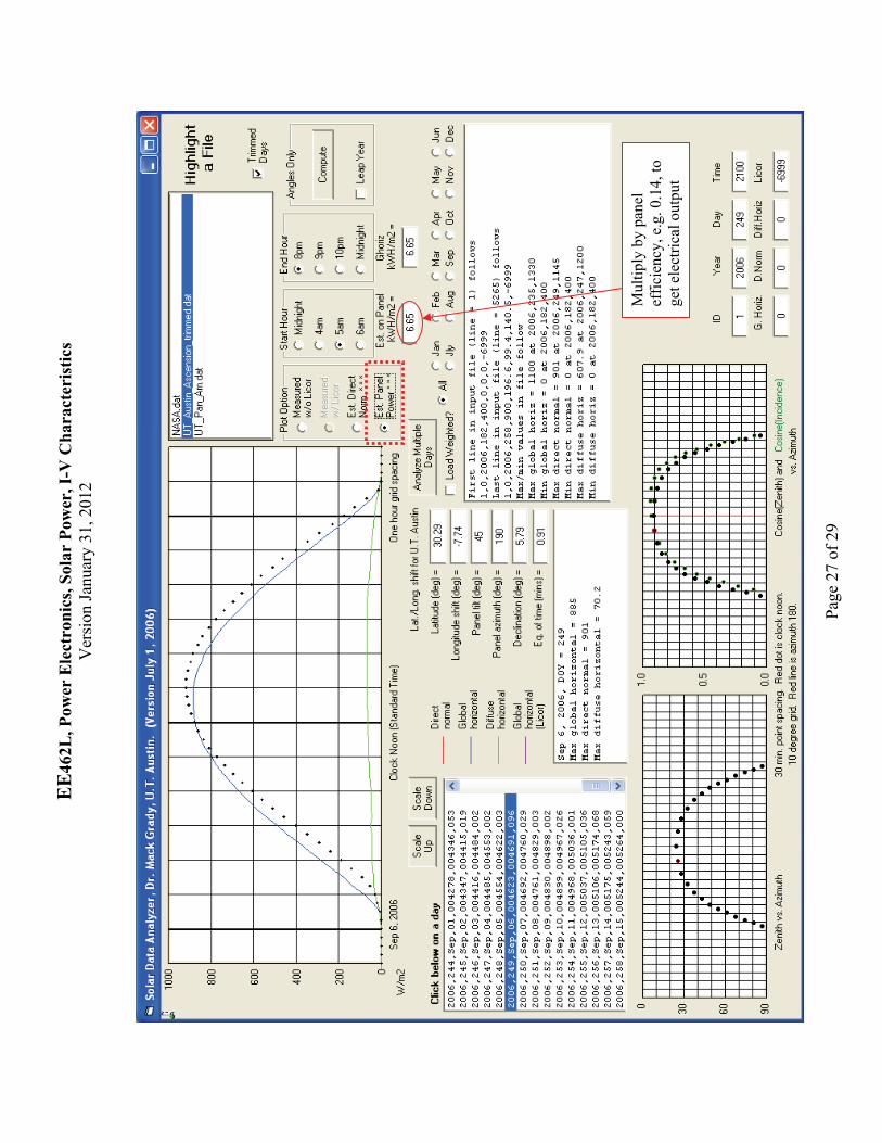
M
ulti
ply
by p
anel
ef
fici
ency
, e.g
. 0.1
4, to
ge
t ele
ctri
cal o
utpu
t
EE
462L
, Pow
er E
lect
ron
ics,
Sol
ar P
ower
, I-V
Ch
arac
teri
stic
s V
ersi
on J
anua
ry 3
1, 2
012
Pag
e 28
of
29
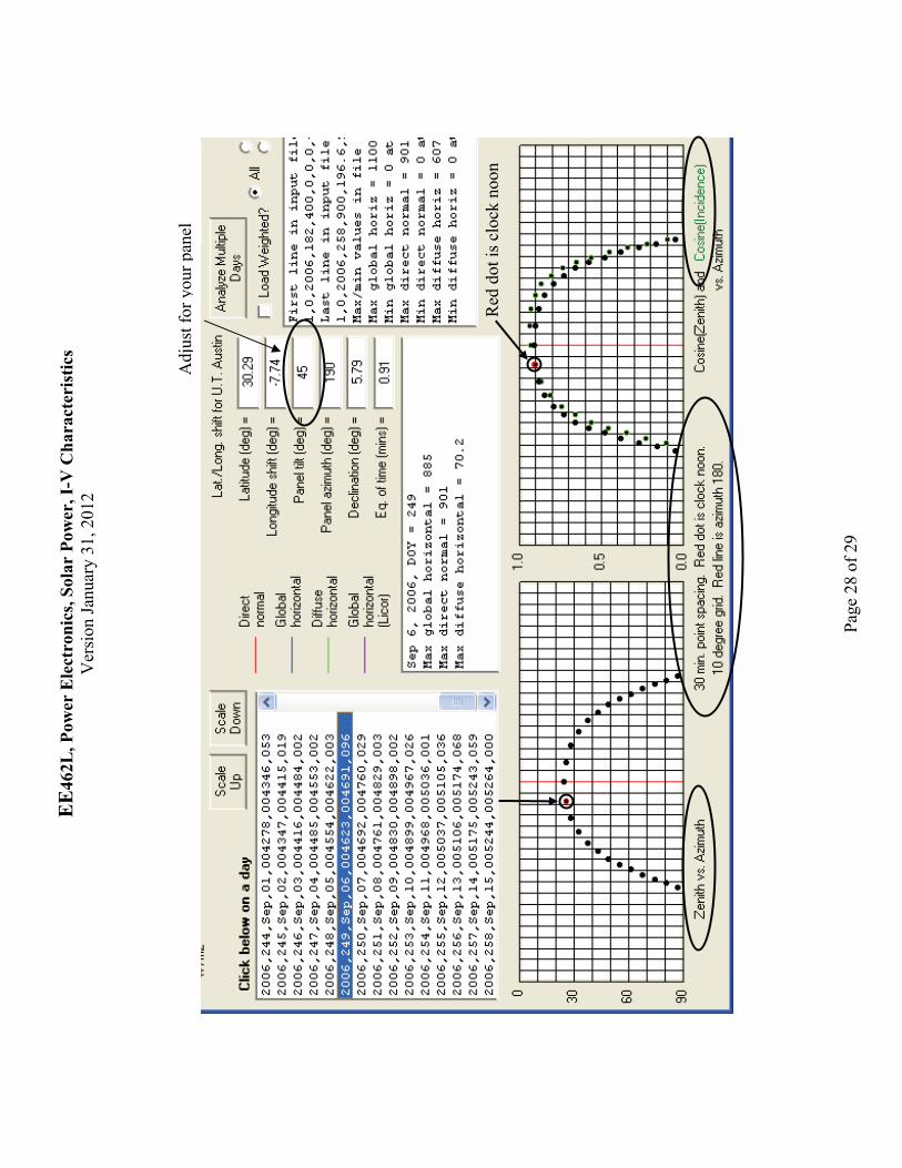
Red
dot
is c
lock
noo
n
Adj
ust f
or y
our
pane
l

EE
462L
, Pow
er E
lect
ron
ics,
Sol
ar P
ower
, I-V
Ch
arac
teri
stic
s V
ersi
on J
anua
ry 3
1, 2
012
Pag
e 29
of
29
Sol
ar a
naly
sis
for
Sep
t. 25
, 200
6. A
ssum
e pa
nels
are
at 3
0º ti
lt, 1
80º
azim
uth.
Inc
iden
t kW
H o
n 1m
2 pan
el (
appr
ox. 1
50W
rat
ed)
is
7.02
kWH
. M
ulti
plyi
ng b
y 0.
14 e
ffic
ienc
y yi
elds
0.9
8 kW
H.
Tha
t cor
resp
onds
to a
bout
6.5
kWH
per
1kW
rat
ed o
f so
lar
pane
ls.
Thu
s, if
a (
non-
air
cond
ition
ed)
hous
e co
nsum
es 2
0 kW
H p
er d
ay, t
hen
abou
t 3kW
of
pane
ls a
re n
eede
d. U
sing
$4.
5 pe
r W
, whi
ch
infl
ates
to a
bout
$7.
0 pe
r W
with
mou
ntin
g an
d el
ectr
onic
s, th
en th
e 3
kW o
f pa
nels
cos
t abo
ut $
21K
.