EE603 Class Notes 10/10/2013 John Stensby Chapter 9 ... · EE603 Class Notes 10/10/2013 John Stensby Updates at 9-1 Chapter 9: Commonly Used Models: Narrow-Band Gaussian Noise and

EE603 Class Notes 10/10/2013 John Stensby

Updates at http://www.ece.uah.edu/courses/ee385/ 9-1

Chapter 9: Commonly Used Models: Narrow-Band Gaussian Noise and Shot Noise

Narrow-band, wide-sense-stationary (WSS) Gaussian noise (t) is used often as a noise

model in communication systems. For example, (t) might be the noise component in the output

of a radio receiver intermediate frequency (IF) filter/amplifier. In these applications, sample

functions of (t) are expressed as

(t) (t)cos t (t)sin t c c s c , (9-1)

where c is termed the center frequency (for example, c could be the actual center frequency of

the above-mentioned IF filter). The quantities c(t) and s(t) are termed the quadrature

components (sometimes, c(t) is known as the in-phase component and s(t) is termed the

quadrature component), and they are assumed to be real-valued.

Narrow-band noise (t) can be represented in terms of its envelope R(t) and phase (t).

This representation is given as

c(t) R(t)cos( t (t)) , (9-2)

where

2 2c s

1s c

R(t) (t) (t)

(t) tan ( (t) / (t)).

(9-3)

Normally, it is assumed that R(t) 0 and – (t) for all time.

Note the initial assumptions placed on (t). The assumptions of Gaussian and WSS

behavior are easily understood. The narrow-band attribute of (t) means that c(t), s(t), R(t)

and (t) are low-pass processes; these low-pass processes vary slowly compared to cosct ; they



are on a vastly different time scale from cosct. Many periods of cosct occur before there is

notable change in c(t), s(t), R(t) or (t).

A second interpretation can be given for the term narrow-band. This is accomplished in

terms of the power spectrum of (t), denoted as S(). By the Wiener-Khinchine theorem,

S() is the Fourier transform of R(), the autocorrelation function for WSS (t). Since (t) is

real valued, the spectral density S() satisfies

( ) 0

( ) ( ).

S

S S

(9-4)

Figure 9-1 depicts an example spectrum of a narrow-band process. The narrow-band attribute

means that S() is zero except for a narrow band of frequencies around c; process (t) has a

bandwidth (however it might be defined) that is small compared to the center frequency c.

Power spectrum S() may, or may not, have ±c as axes of local symmetry. If c is

an axis of local symmetry, then

S S ( ) ( ) c c (9-5)

for 0 < < c, and the process is said to be a symmetrical band-pass process (Fig. 9-1 depicts a

symmetrical band-pass process). It must be emphasized that the symmetry stated by the second

of (9-4) is always true (i.e., the power spectrum is even); however, the symmetry stated by (9-5)

Rad/Sec

S()

-c c

wat

ts/H

z

Fig. 9-1: Example spectrum of narrow-band noise.



may, or may not, be true. As will be shown in what follows, the analysis of narrow-band noise is

simplified if (9-5) is true.

To avoid confusion when reviewing the engineering literature on narrow-band noise, the

reader should remember that different authors use slightly different definitions for the cross-

correlation of jointly-stationary, real-valued random processes x(t) and y(t). As used here, the

cross-correlation of x and y is defined as Rxy( ) E[x(t+)y(t)]. However, when defining Rxy,

some authors shift (by ) the time variable of the function y instead of the function x.

Fortunately, this possible discrepancy is accounted for easily when comparing the work of

different authors.

(t) has Zero Mean

The mean of (t) must be zero. This conclusion follows directly from

c c s cE[ (t)] E[ (t)]cos t E[ (t)]sin t . (9-6)

The WSS assumption means that E[(t)] must be time invariant (constant). Inspection of (9-6)

leads to the conclusion that E[c] = E[s] = 0 so that E[] = 0.

Quadrature Components In Terms of and ̂

Let the Hilbert transform of WSS noise (t) be denoted in the usual way by the use of a

circumflex; that is, (t) denotes the Hilbert transform of (t) (see Appendix 9A for a discussion

of the Hilbert transform). The Hilbert transform is a linear, time-invariant filtering operation

applied to (t); hence, from the results developed in Chapter 7, (t) is WSS.

In what follows, some simple properties are needed of the cross correlation of (t) and

(t) . Recall that (t) is the output of a linear, time-invariant system that is driven by (t). Also

recall that techniques are given in Chapter 7 for expressing the cross correlation between a

system input and output. Using this approach, it can be shown easily that



ˆ

ˆ

ˆ ˆ

ˆ

ˆˆR ( ) E[ (t ) (t)] R ( )

ˆˆR ( ) E[ (t ) (t)] R ( )

R (0) R (0) 0

R ( ) R ( ) .

(9-7)

Equation (9-1) can be used to express (t) . The Hilbert transform of the noise signal can

be expressed as

(t) (t) cos t (t) sin t (t) cos t (t) sin t

(t) sin t (t) cos t .

c c s c c c s c

c c s c

(9-8)

This result follows from the fact that c is much higher than any frequency component in c or

s so that the Hilbert transform is only applied to the high-frequency sinusoidal functions (see

Appendix 9A).

The quadrature components can be expressed in terms of and . This can be done by

solving (9-1) and (9-8) for

c c c

s c c

(t) (t)cos t (t)sin t

(t) (t)cos t (t)sin t .

(9-9)

These equations express the quadrature components as a linear combination of Gaussian .

Hence, the components c and s are Gaussian. In what follows, Equation (9-9) will be used to

calculate the autocorrelation and crosscorrelation functions of the quadrature components. It

will be shown that the quadrature components are WSS and that c and s are jointly WSS.

Furthermore, WSS process (t) is a symmetrical band-pass process if, and only if, c and s are



uncorrelated for all time shifts.

Relationships Between Autocorrelation Functions R , Rc and Rs

It is easy to compute, in terms of R, the autocorrelation of the quadrature components.

Use (9-9) and compute the autocorrelation

R ( ) E[ (t) (t )]

E[ (t) (t )]cos t cos (t ) E[ (t) (t )]sin t cos (t )

E[ (t) (t )]cos t sin (t ) E[ (t) (t )]sin t sin (t ) .

c c c

c c c c

c c c c

(9-10)

This last result can be simplified by using (9-7) to obtain

R ( ) R ( )[cos t cos (t ) sin t sin (t )]

R ( )[cos t sin (t ) sin t cos (t )] ,

c c c c c

c c c c

a result that can be expressed as

R ( ) R ( )cos R ( )sin . c c c (9-11)

The same procedure can be used to compute an identical result for Rs ; this leads to the

conclusion that

c sR ( ) R ( ) (9-12)

for all . Note that c and s are zero mean, Gaussian, and wide-sense stationary.

Equations (9-11) and (9-12) allow the computation of cR and Rs given only R .

However, given only cR and/or Rs , we do not have enough information to compute R



(what is missing?).

A somewhat non-intuitive result can be obtained from (9-11) and (9-12). Set = 0 in the

last two equations to conclude that

c sR (0) R (0) R (0) , (9-13)

an observation that leads to

2 2c s

c s

E[ (t)] E[ (t)] E[ (t)]

Avg Pwr in (t) = Avg Pwr in (t) = Avg Pwr in (t).

(9-14)

The frequency domain counterpart of (9-11) relates the spectrums S , Sc and Ss .

Take the Fourier transform of (9-11) to obtain

c cc s

c c c c

c c c c

1( ) ( ) ( ) ( )

2

1sgn( ) ( ) sgn( ) ( )

2

1 11 sgn( ) ( ) 1 sgn( ) ( )

2 2

S S S S

S S

S S

(9-15)

Since c and s are low-pass processes, Equation (9-15) can be simplified to produce

c c c cc s( ) ( ) ( ) ( ),

0, otherwise,

S S S S

(9-16)

a relationship that is easier to grasp and remember than is (9-11).



Equation (9-16) provides an easy method for obtaining Sc and/or sS given only S .

First, make two copies of S. Shift the first copy to the left by c, and shift the second copy

to the right by c. Add together both shifted copies, and truncate the sum to the interval c

c to get Sc . This “shift and add” procedure for creating Sc is illustrated by Fig. 9-2.

Given only S, it is always possible to determine Sc (which is equal to sS ) in this manner.

The converse is not true; given only Sc , it is not always possible to create S (Why? Think

cc

S

Sc) , < c

cc

Sc) , < c

cc

Sc = Sc) + Sc) , < c

c c

Fig. 9-2: Creation of cS from shifting and adding copies of S .



about the fact that S c( ) must be even, but S may not satisfy (9-5);what is missing?).

Crosscorrelation R c s

It is easy to compute the cross-correlation of the quadrature components. From (9-9) it

follows that

R ( ) E[ (t ) ( )]

E[ (t ) (t)]cos (t )cos t E[ (t ) (t)]cos (t )sin t

E[ (t ) (t)]sin (t )cos t E[ (t ) (t)]sin (t )sin t .

c s c s

c c c c

c c c c

t

(9-17)

By using (9-7), Equation (9-17) can be simplified to obtain

R ( ) R ( )[ sin t cos (t ) cos t sin (t )]

R ( )[cos t cos (t ) sin t sin (t )] ,

c s c c c c

c c c c

a result that can be written as

R ( ) R ( )sin R ( )cos c s c c . (9-18)

The cross-correlation of the quadrature components is an odd function of . This follows

directly from inspection of (9-18) and the fact that an even function has an odd Hilbert

transform. Finally, the fact that this cross-correlation is odd implies that R ( ) c s 0 = 0; taken at

the same time, the samples of c and s are uncorrelated and independent. However, as

discussed below, the quadrature components c(t1) and s(t2) may be correlated for t1 t2.

The autocorrelation R of the narrow-band noise can be expressed in terms of the

autocorrelation and cross-correlation of the quadrature components c and s . This important

result follows from using (9-11) and (9-18) to write



c s

c

c c

c c

R ( ) R ( )sin cos

ˆR ( ) R ( )cos sin

.

Invert this to obtain

c s

c

c c

c c

R ( )R ( ) sin cos

ˆ R ( )R ( ) cos sin

, (9-19)

which yields the desired formula

R ( ) R ( )cos R ( )sin c c c s c . (9-20)

Equation (9-20) shows that both R ( ) c and R ( ) c s are necessary to compute R .

Comparison of (9-16) with the Fourier transform of (9-20) reveals an “unsymmetrical”

aspect in the relationship between S , Sc and Ss . In all cases, both Sc and Ss can be

obtained by simple translations of S as is shown by (9-16). However, in general, S cannot be

expressed in terms of a similar, simple translation of Sc (or Ss ), a conclusion reached by

inspection of the Fourier transform of (9-20). But, as shown next, there is an important special

case where R ( ) c s is identically zero for all , and S can be expresses as simple translations

of Sc .

Symmetrical Bandpass Processes

Narrow-band process (t) is said to be a symmetrical band-pass process if

S S ( ) ( ) c c (9-21)

for 0 < < c. Such a bandpass process has its center frequency c as an axis of local



symmetry. In nature, symmetry usually leads to simplifications, and this is true of Gaussian

narrow-band noise. In what follows, we show that the local symmetry stated by (9-21) is

equivalent to the condition R ( ) c s 0 for all (not just at = 0).

The desired result follows from inspecting the Fourier transform of (9-18); this transform

is the cross spectrum of the quadrature components, and it vanishes when the narrow-band

process has spectral symmetry as defined by (9-21). To compute this cross spectrum, first note

the Fourier transform pairs

R ( ) ( )

R̂ ( ) jsgn( ) ( ) ,

S

S

(9-22)

where

1 for 0sgn( )

1 for 0

> (9-23)

is the commonly used “sign” function. Now, use Equation (9-22) and the Frequency Shifting

Theorem to obtain the Fourier transform pairs

R ( ) sin ( ) ( )

R ( ) cos Sgn( ) ( ) Sgn( ) ( ) .

c c c

c c c c c

j

1

2

1

2

S S

S Sj

(9-24)

Finally, use this last equation and (9-18) to compute the cross spectrum



S

S S

c s c s

j c c c c

( ) [ R ( )]

( )[ Sgn( )] ( )[ Sgn( )] .

F

1

21 1

(9-25)

Figure 9-3 depicts example plots useful for visualizing important properties of (9-25).

From parts b) and c) of this plot, note that the products on the right-hand side of (9-25) are low

pass processes. Then it is easily seen that

c

c c c cc s

c

0 ,

( ) j[ ( ) ( )],

0 , .

S S S (9-26)

S()

-c c-2c 2c

a)

L LU U

S(-c)

-c c-2c 2c

1-Sgn(-c)

b)

L LU U

S(+c)

-c c-2c 2c

1+Sgn(+c)

c)

L LU U

Figure 9-3: Symmetrical bandpass processes have c(t1) and s(t2) uncorrelated for all t1 and t2.



Note that S c s ( ) 0 is equivalent to the narrow-band process satisfying the symmetry

condition (9-21). On Fig. 9-3, the symmetry condition (9-21) implies that the spectral

components labeled with U can be obtained from those labeled with L by a simple folding

operation. And, when the spectrums are subtracted as required by (9-26), the portion labeled U

(alternatively, L ) on Fig. 9-3c will cancel the portion labeled L (alternatively, U ) on Fig 9-3b.

Finally, since the cross spectrum is the Fourier transform of the cross-correlation, S c s ( ) 0

is both necessary and sufficient for c(t1) and s(t2) to be uncorrelated for all t1 and t2 (not just t1

= t2).

System analysis is simplified greatly if the noise encountered has a symmetrical

spectrum. Under these conditions, the quadrature components are uncorrelated, and (9-20)

simplifies to

R ( ) R ( )cos c c . (9-27)

Also, the spectrum S of the noise is obtained easily by scaling and translating Sc F [R ]c

as shown by

S S S ( ) [ ( ) ( )] 1

2 c c c c . (9-28)

This result follows directly by taking the Fourier transform of (9-27). Hence, when the process

is symmetrical, it is possible to express S in terms of a simple translations of Sc(see the

comment after (9-20)). Finally, for a symmetrical bandpass process, Equation (9-16) simplifies

to

S S S c s

2( ) ( ) ( ),

,

c c c

otherwise0. (9-29)



Example 9-1: Figure 9-4 depicts a simple RLC bandpass filter that is driven by white Gaussian

noise with a double sided spectral density of N0/2 watts/Hz. The spectral density of the output is

given by

S

( ) ( )

( )

( )

NH j

N j

jbp

c

0 2 0 0

02 2

2

2 2

2, (9-30)

where 0 = R/2L, c = (n2 - 0

2)1/2 and n = 1/(LC)1/2. In this result, frequency can be

normalized, and (9-30) can be written as

S

( )

( )

( )

N j

j0 0

02

2

2

2

1, (9-31)

where 0 = 0/c and = /c. Figure 9-5 illustrates a plot of the output spectrum for o = .5;

note that the output process is not symmetrical. Figure 9-6 depicts the spectrum for o = .1 (a

much “sharper” filter than the o = .5 case). As the circuit Q becomes large (i.e., o becomes

small), the filter approximates a symmetrical filter, and the output process approximates a

symmetrical bandpass process.

Envelope and Phase of Narrow-Band Noise

Zero-mean quadrature components c(t) and s(t) are jointly Gaussian, and they have the

same variance 2 = R R Rc s ( ) ( ) ( )0 0 0 . Also, taken at the same time t, they are

L C

R

+

-

+S() = N0/2watts/Hz(WGN)

Figure 9-4: A simple band-pass filter driven by white Gaussian noise (WGN).



independent. Hence, taken at the same time, processes c(t) and s(t) are described by the joint

density

f c sc s( , ) exp

LNMM

OQPP

1

2 22

2 2

2. (9-32)

We are guilty of a common abuse of notation. Here, symbols c and s are used to denote

random processes, and sometimes they are used as algebraic variables, as in (9-32). However,

always, it should be clear from context the intended use of c and s.

The narrow-band noise signal can be represented as

c c s c

1 c 1

(t) (t) cos t (t)sin t

(t) cos( t (t))

(9-33)

where

-2 -1 0 1 2(radians/second)

0.10.20.30.40.50.60.70.80.91.0

S()

Figure 9-5: Output Spectrum for o = .5

-2 -1 0 1 2(radians/second)

0.10.20.30.40.50.60.70.80.91.0

S()

Figure 9-6: Output Spectrum for o = .1



2 21 c s

1 s1 1

c

(t) (t) (t)

(t)(t) Tan , - < ,

(t)

(9-34)

are the envelope and phase, respectively. Note that (9-34) describes a transformation of c(t)

and s(t). The inverse is given by

c

s

1

1

cos( )

sin( )

1

1

(9-35)

The joint density of 1 and can be found by using standard techniques. Since (9-35) is

the inverse of (9-34), we can write

c 1 1

s 1 1

c s1 1 c s cos1 1

sin

( , )f ( , ) f ( , )

( , )

(9-36)

c s 1 1 11

1 1 11 1

( , ) cos sindet sin cos( , )

(again, the notation is abusive). Finally, substitute (9-32) into (9-36) to obtain

2 2 211 1 1 1 12 2

2112 2

1f ( , ) exp (sin cos )

2 2

1exp ,

2 2

. (9-37)

for 1 0 and - < . Finally, note that (9-37) can be represented as



f f( , ) ( )f( ) 1 1 1 1 , (9-38)

where

f U( ) exp ( )

112 2 1

21

1

2

LNM

OQP

(9-39)

describes a Rayleigh distributed envelope, and

f( ) , 1 1 1

2 - < (9-40)

describes a uniformly distributed phase. Finally, note that the envelope and phase are

independent. Figure 9-7 depicts a hypothetical sample function of narrow-band Gaussian noise.

Envelope and Phase of a Sinusoidal Signal Plus Noise - the Rice Density Function

Many communication problems involve deterministic signals embedded in random noise.

The simplest such combination of signal and noise is that of a constant frequency sinusoid added

to narrow-band Gaussian noise. In the 1940s, Steven Rice analyzed this combination and

published his results in the paper Statistical Properties of a Sine-wave Plus Random Noise, Bell

System Technical Journal, 27, pp. 109-157, January 1948. His work is outlined in this section.

Fig. 9-7: A hypothetical sample function of narrow-band Gaussian noise. The envelope is Rayleigh and the phase is uniform.



Consider the sinusoid

0 c 0 0 0 c 0 0 cs(t) A cos( t ) A cos cos t A sin sin t , (9-41)

where A0, c, and 0 are known constants. To signal s(t) we add noise (t) given by (9-1), a

zero-mean WSS band-pass process with power 2 = E[2] = E[c2] = E[s

2]. This sum of signal

and noise can be written as

0 0 c c 0 0 s c

2 c 2

s(t) + (t) [A cos (t)]cos t [A sin (t)]sin t

(t)cos[ t ] ,

(9-42)

where

2 22 0 0 c 0 0 s

1 0 0 s2 2

0 0 c

(t) [A cos (t)] [A sin (t)]

A sin (t)(t) tan , ,

A cos (t)

(9-43)

are the envelope and phase, respectively, of the signal+noise process. Note that the quantity

2 20(A / 2 ) / is the signal-to-noise ratio, a ratio of powers.

Equation (9-43) represents a transformation from the components c and s into the

envelope 2 and phase 2. The inverse of this transformation is given by

c 2 2 0 0

s 2 2 0 0

(t) (t)cos (t) A cos

(t) (t)sin (t) A sin .

(9-44)



Note that constants A0cos0 and A0sin0 only influence the means of 2cos(2) and 2sin(2)

(remember that both c and s have zero mean!). In the remainder of this section, we describe

the statistical properties of envelope 2 and phase 2.

At the same time t, processes c(t) and s(t) are statistically independent (however, for

0, c(t) and s(t+) may be dependent). Hence, for c(t) and s(t) we can write the joint

density

f c sc s( , )

exp[ ( ) / ]

2 2 2

22

2 (9-45)

(we choose to abuse notation for our convenience: c and s are used to denote both random

processes and, as in (9-45), algebraic variables).

The joint density f( 2) can be found by transforming (9-45). To accomplish this, the

Jacobian

c s 2 2 22

2 2 22 2

( , ) cos sindet sin cos( , )

(9-46)

can be used to write the joint density

c 2 2 0 0

s 2 2 0 0

c s2 2 c s

cos A cos2 2sin A sin

( , )f ( , ) f ( , )

( , )

(9-47)

22 22 1

2 2 2 0 2 0 22 2f ( , ) exp [ 2A cos( ) A ] U( )

2

2 0 .

Now, the marginal density f() can be found by integrating out the 2 variable to obtain



2

22 2 20

22 22 0 21 12 0 2 2 0 22 2 202

f ( ) f ( , ) d

Aexp [ A ] U( ) exp{ cos( )}d .

2

(9-48)

This result can be written by using the tabulated function

I d01

2 0

2( ) exp{ cos( )}

z , (9-49)

the modified Bessel function of order zero. Now, use definition (9-49) in (9-48) to write

f I A UA

( ) exp [ ] ( )

2

22 0

12

22

02

22 0

2 2 FH IK RSTUVW

, (9-50)

a result known as the Rice probability density. As expected, 0 does not enter into f(2).

Equation (9-50) is an important result. It is the density function that statistically

describes the envelope 2 at time t; for various values of A0/, the function f(2) is plotted on

Figure 9-8 (the quantity 2 20(A / 2) / is the signal-to-noise ratio). For A0/ = 0, the case of no

sinusoid, only noise, the density is Rayleigh. For large A0/ the density becomes Gaussian. To

observe this asymptotic behavior, note that for large the approximation

Ie

02

( ) ,

>> 1, (9-51)

becomes valid. Hence, for large 2A0/ Equation (9-50) can be approximated by

fA

A U( ) exp [ ] ( )

22

02

12

2 02

22

2 RSTUVW

. (9-52)



For A0 >> , this function has a very sharp peak at 2 = A0, and it falls off rapidly from its peak

value. Under these conditions, the approximation

f A( ) exp [ ] 2 21

22 0

21

22 RST

UVW (9-53)

holds for values of 2 near A0 (i.e., 2 A0) where f(2) is significant. Hence, for large A0/,

envelope 2 is approximately Gaussian distributed.

The marginal density f(2) can be found by integrating 2 out of (9-47). Before

integrating, complete the square in 2, and express (9-47) as

f A UA( , ) exp [ cos( )] exp sin ( ) ( )

22

21

2 2 02

22

22

20

2

2 2 2 0 2 0

RSTUVW

{ } . (9-54)

0 1 2 3 4 5 6

0.0

0.1

0.2

0.3

0.4

0.5

0.6

0.7

0.8

f

(2)

A0/ = 0

A0/ = 1A0/ = 2

A0/ = 3A0/ = 4

Figure 9-8: Rice density function for sinusoid plus noise. Plotsare given for several values of A0/. Note that f is approximately Rayleigh for small, positive A0/ density f is approximately Gaussian for large A0/.



Now, integrate 2 out of (9-54) to obtain

2 2 2 20

2A 22 1202 0 2 0 22 0 222 0 22

f ( ) f ( , )d

exp exp [ A cos( )] d .sin ( )2

(9-55)

On the right-hand-side of (9-55), the integral can be expressed as the two integrals

220

12 2 0

22

2 020

12 2 0

22

02

12 2 0

220

2

2

4

2

2

2

2

zz

z

exp [ cos( )]

{ cos( )}exp [ cos( )]

cos( )exp [ cos( )]

A d

AA d

AA d

2 0

2 02 0

2 02 0

{ }

{ }

{ }

(9-56)

After a change of variable = [2 - A0cos(2 - 0)]2 , the first integral on the right-hand-side of

(9-56) can be expressed as

2 2A cos ( )00

22 0 2 0 12 0 2 0 2220 2

22 22

2 2A cos ( )2 0022

2{ A cos( )}exp [ A cos( )] d

4

1exp[ ]d

4

1exp .

2

(9-57)

After a change of variable = [2 - A0cos(2 - 0)]/, the second integral on the right-hand-side

of (9-56) can be expressed as



0

0

212 0 2 0 220 2

212(A / )cos[ ]2 0

(A / )cos[ ] 22 0 12

A02 0

1exp [ A cos( )] d

2

1exp d

2

11 exp d

2

F( cos[ ]),

(9-58)

where

F x dx

( ) exp z1

2 2

2

is the distribution function for a zero-mean, unit variance Gaussian random variable (the identity

F(-x) = 1 - F(x) was used to obtain (9-58)).

Finally, we are in a position to write f(), the density function for the instantaneous

phase. This density can be written by using (9-57) and (9-58) in (9-55) to write

2A02 22

2 AA0 2 0 0202 02 022

1f ( ) exp

2

A cos( )exp F( cos[ ])sin ( )

2

, (9-59)

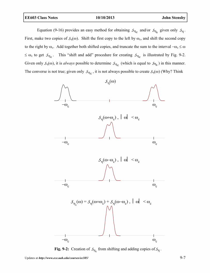
the density function for the phase of a sinusoid embedded in narrow-band noise. For various

values of SNR and for 0 = 0, density f() is plotted on Fig. 9-9. For a SNR of zero (i.e., A0 =

0), the phase is uniform. As SNR A02/2 increases, the density becomes more sharply peaked (in

general, the density will peak at 0, the phase of the sinusoid). As SNR A02/2 approaches

infinity, the density of the phase approaches a delta function at 0.



Shot Noise

Shot noise results from filtering a large number of independent and randomly-occuring-

in-time impulses. For example, in a temperature-limited vacuum diode, independent electrons

reach the anode at independent times to produce a shot noise process in the diode output circuit.

A similar phenomenon occurs in diffusion-limited pn junctions. To understand shot noise, you

must first understand Poisson point processes and Poisson impulses.

Recall the definition and properties of the Poissson point process that was discussed in

Chapters 2 and 7 (also, see Appendix 9-B). The Poisson points occur at times ti with an average

density of d points per unit length. In an interval of length , the number of points is distributed

with a Poisson density with parameter d.

Use this Poisson process to form a sequence of Poisson Impulses, a sequence of impulses

located at the Poisson points and expressed as

Phase Angle 2

0.0

0.2

0.4

0.6

0.8

1.0

1.2

1.4

1.6

1.8

2.0

f (

2)

A0/ = 0 A0/ = 1

A0/ = 2

A0/ = 4

0 /2-/2-

Figure 9-9: Density function for phase of signal plus noise A0cos(0t+0) + {c(t)cos(0t) - s(t)sin(0t)} for the case 0 = 0.



ii

z(t) (t t ) , (9-60)

where the ti are the Poisson points. Note that z(t) is a generalized random process; like the delta

function, it can only be characterized by its behavior under an integral sign. When z(t) is

integrated, the result is the Poisson random process

t

0

(0, t), t 0

x(t) z( )d 0, t 0

- (0, t) t 0,

n

n

(9-61)

where n(t1,t2) is the number of Poisson points in the interval (t1,t2]. Likewise, by passing the

Poisson process x(t) through a generalized differentiator (as illustrated by Fig. 9-10), it is

possible to obtain z(t).

The mean of z(t) is simply the derivative of the mean value of x(t). Since E[x(t)]=dt, we

can write

z dd

E[z(t)] E[x(t)]dt

. (9-62)

This formal result needs a physical interpretation. One possible interpretation is to view z as

...... ......d/dt

x(t) z(t)

Poisson ImpulsesPoisson Process

Figure 9-10: Differentiate the Poisson Process to get Poisson impulses.



t / 21 1z d dt tt / 2t t

limit z( )d limit t random fluctuation with increasing t

. (9-63)

For large t, the integral in (9-63) fluctuates around mean dt with a variance of dt (both the

mean and variance of the number of Poisson points in (-t/2, t/2] is dt). But, the integral is

multiplied by 1/t; the product has a mean of d and a variance like d/t. Hence, as t becomes

large, the random temporal fluctuations become insignificant compared to d, the infinite-time-

interval average z.

Important correlations involving z(t) can be calculated easily. Because Rx(t1,t2) = 2d t1t2

+ dmin(t1,t2) (see Chapter 7), we obtain

2xz 1 2 x 1 2 d 1 d 1 2

2

2z 1 2 xz 1 2 d d 1 2

1

R (t , t ) R (t , t ) t U(t t )t

R (t , t ) R (t , t ) (t t ) .t

(9-64)

Note that z(t) is wide-sense stationary but x(t) is not. The Fourier transform of Rz() yields

2z d d( ) 2 ( ) S , (9-65)

the power spectrum of the Poisson impulse process.

Let h(t) be a real-valued function of time and define

ii

s(t) h(t t ) , (9-66)

a sum known as shot noise. The basic idea here is illustrated by Fig. 9-11. A sequence of

functions described by (9-60) (i.e., process z(t)) is input to system h(t) to form output shot noise

process s(t). The idea is simple: process s(t) is the output of a system activated by a sequence of



impulses (that model electrons arriving at an anode, for example) that occur at the random

Poisson points ti.

Determined easily are the elementary properties of shot noise s(t). Using the method

discussed in Chapter 7, we obtain the mean

s d d0E s(t) E z(t) h(t) h(t) E z(t) h(t)dt H(0)

. (9-67)

Shot noise s(t) has the power spectrum

2 2 22 2 2

s z d d s d( ) H( ) ( ) 2 H (0) ( ) H( ) 2 ( ) H( ) S S . (9-68)

Finally, the autocorrelation is

2-1 2 2 j 2 2ds s d d dR ( ) = ( ) H (0) H( ) e d H (0) ( )

2

SF , (9-69)

where

2 j1( ) H( ) e d h(t)h(t )dt

2

. (9-70)

From (9-67) and (9-69), shot noise has a mean and variance of

ti-1 ti+1 ti+2ti ti-1 ti+1 ti+2ti

...... ......h(t)

z(t) s(t) = h(t)z(t)

h(t)

Poisson Impulses Shot Noise

Figure 9-11: Converting Poisson impulses z(t) into shot noise s(t)



s d

22 2 2 2 ds d d d d

= H(0)

= [ H (0) + (0)] - [ H(0)] (0) H( ) d ,2

(9-71)

respectively (Equation (9-71) is known as Campbell’s Theorem).

Example: Let h(t) = e-tU(t) so that H() = 1/( + j), ( ) e / 2 and

2

d d ds s

22 d d ds s 2 2

E[s(t)] R ( ) e2

( ) 2 ( )2

S

(9-72)

First-Order Density Function for Shot Noise

In general, the first-order density function fs(x) that describes shot noise s(t) cannot be

calculated easily. Before tackling the difficult general case, we first consider a simpler special

case where it is assumed that h(t) is of finite duration T. That is, we assume initially that

h(t) 0, t 0 and t T . (9-73)

Because of (9-73), shot noise s at time t depends only on the Poisson impulses in the

interval (t - T, t]. To see this, note that

i

i ii t T t t

s(t) h(t ) ( t )d h(t t )

, (9-74)

so that only the impulses in the “moving window” (t - T, t] influence the output at time t. Let

random variable nT denote the number of Poisson impulses during (t - T, t]. From Chapter 1, we



know that

dk

T d( T)[ k] e

k!

TP n . (9-75)

Now, the Law of Total Probability (see Ch. 1 and Ch. 2 of these notes) can be applied to write

the first-order density function of the shot noise process s(t) as

dk

T ds s s

k 0 k 0

( T)f (x) f (x k) [ k] f (x k)e

k!

T T Tn P n n (9-76)

(note that fs(x) is independent of absolute time t). We must find fs(xnT = k), the density of shot

noise s(t) conditioned on there being exactly k Poisson impulses in the interval (t - T, t].

When nT = k = 0, there are no Poisson points in (t - T, t], and we have

0 sg (x) f (x = 0) = (x) Tn (9-77)

since the output is zero.

For each fixed value of k 1 that is used on the right-hand-side of (9-76), conditional

density fs(xnT = k) describes the filter output due to an input of exactly k impulses on (t - T, t].

That is, we have conditioned on there being exactly k impulses in (t - T, t]. As a result of the

conditioning, the k impulse locations can be modeled as k independent, identically distributed

(iid) random variables (all locations ti, 1 i k, are uniform on the interval).

For the case k = 1, at any fixed time t, fs(xnT = 1) is actually equal to the density g1(x)

of the random variable

1 1x (t) h(t t ) , (9-78)



where random variable t1 is uniformly distributed on (t - T, t] so that t - t1 is uniform on [0,T).

That is, g1(x) fs(xnT = 1) describes the result that is obtained by transforming a uniform

density (used to describe t - t1) by the transformation h(t - t1).

Convince yourself that density g1(x) = fs(xnT = 1) does not depend on time. Note that

for any given time t, random variable t1 is uniform on (t-T, t] so that t - t1 is uniform on [0,T).

Hence, the quantity x1(t) h(t-t1) is assigned values in the set {h() : 0 < T}, the assignment

not depending on t. Hence, density g1(x) fs(xnT = 1) does not depend on t.

The density fs(xnT = 2) can be found in a similar manner. Let t1 and t2 denote

independent random variables, each of which is uniformly distributed on (t - T, t], and define

2 1 2x (t) h(t t ) h(t t ) . (9-79)

At fixed time t, the random variable x2(t) is described by the density g2(x) fs(xnT = 2) = g1g1

(i.e., the convolution of g1 with itself) since h(t - t1) and h(t - t2) are independent and identically

distributed with density g1.

The general case fs(xnT = k) is similar. Let ti, 1 i k, denote independent random

variables, each uniform on (t - T, t]. At fixed time t, the density that describes

k 1 2 kx (t) h(t t ) h(t t ) h(t t ) (9-80)

is

k s 1 1 1

k 1 convolutions

g (x) f (x = k) = g (x) g (x) g (x)

Tn , (9-81)

the density g1 convolved with itself k-1 times.

The desired density can be expressed in terms of results given above. Simply substitute



(9-81) into (9-76) and obtain

dk

T ds k

k 0

( T)f (x) e g (x)

k!

. (9-82)

Convergence is fast, and (9-82) is useful for computing the density fs when dT is small (the case

for low density shot noise), say on the order of 1, so that, on the average, there are only a few

Poisson impulses in the interval (t - T, t]. For the case of low density shot noise, (9-82) cannot

be approximated by a Gaussian density.

fs(x) For An Infinite Duration h(t)

The first-order density function fs(x) is much more difficult to calculate for the general

case where h(t) is of infinite duration (but with finite time constants). In what follows, assume

that infinite duration h(t) is significant only over 0 t < 5max, where max is the filter’s dominant

time constant. We show that shot noise is approximately Gaussian distributed when d is large

compared to the time interval over which h(t) is significant (so that, on the average, many

Poisson impulses are filtered to form s(t)).

To establish this fact, consider first a finite duration interval (-T/2, T/2), and let random

variable nT, described by (9-75), denote the number of Poisson impulses that are contained in the

interval. Located in (-T/2, T/2), denote the nT Poison Impulse locations as tk, 1 k nT. Use

these nT impulse locations to define time-limited shot noise

T kk 1

s (t) h(t t ), t

Tn

. (9-83)

Shot noise s(t) is the limit of sT(t) as T approaches infinity.



In our analysis of shot noise s(t), we first consider the characteristic function

Tj sj ss

T( ) E e limit E e

. (9-84)

For finite T, characteristic function Tj sE e depends on t (which is suppressed in the notation).

However, shot noise is wide-sense stationary, so s() should be free of t. Now, write the

characteristic function of sT as

T Tj s j s

k 0

E e E e k k

T Tn P n , (9-85)

where P[nT = k] is given by (9-75). In the conditional expectation used on the right-hand-side

of (9-85), output sT results from filtering exactly k impulses (this is different from the not-

conditioned-on-anything sT that appears on the left-hand-side of (9-85)). We model the impulse

locations as k independent, identically distributed (iid – they are uniform on (-T/2, T/2)) random

variables. As a result, the terms h(t - ti) in sT(t) are independent so that

T Tk

j s j sE e k E e 1 T Tn n , (9-86)

where

TT/2j s j h(t x)T/2

1E e 1 e dx,

T

Tn (9-87)

since each ti is uniformly distributed on (-T/2, T/2). Finally, by using (9-84) through (9-87), we

can write



T T

d

d

j s j ss

T T k 0

kkT/2 Tj h(t x) dT/2T k 0

kT/2 j h(t x)dT T/2

T k 0

( ) limit E e limit E e k k

( T)1limit e dx e

T k!

e dxlimit e

k!

T Tn P n

(9-88)

For finite T, the quantity T / 2 j h(t x)T / 2

e dx depends on t. However, the quantity j h(t x)e dx

does not depend on t. Recalling the Taylor series of the exponential function, we can write

(9-88) as

T / 2 j h(t x) j h(t x)s d d dT / 2T( ) limit exp{ T}exp e dx exp e 1 dx

, (9-89)

a general formula for the characteristic function of the shot noise process.

In general, Equation (9-89) is impossible to evaluate in closed form. However, this

formula can be used to show that shot noise is approximately Gaussian distributed when d is

large compared to the time constants in h(t) (i.e., compared to the time duration where h(t) is

significant).

This task will be made simpler if we “center” and normalize s(t). Define

d

d

s(t)- H(0)(t)

s , (9-90)

so that



E 0

R ( ) ( ) h(t)h(t )dt

s

s

. (9-91)

(see (9-67) and (9-69)). The characteristic functions of s and s are related by

j dd s d

d

s - H(0)( ) E e E exp j exp j H(0) ( )

ss . (9-92)

Use (9-89) and H(0) h(t x)dx

on the right-hand-side of (9-92) to write

d d

j jd( ) exp exp h(t x) 1 h(t x) dx

s . (9-93)

Now, in the integrand of (9-93), expand the exponential in a power series, and cancel out the

zero and first-order terms to obtain

k k

k

k k( j ) ( j )

d dk! k!d dk 2 k 2

k( j )2 2

d k! kk 3 d

h(t x) h(x)( ) exp dx exp dx

h (x)dx1exp h (x)dx exp .

2

s

(9-94)

As d approaches infinity, (i.e., becomes large compared to the time constants in low-pass filter

h(t)), Equation (9-94) approaches the characteristic function of a Gaussian process.

To see this, let max be the dominant (i.e., largest) time constant in low-pass filter h(t).

There exists constant M such that (note that h is causal)



x /h(x) M e U(x) max (9-95)

(max is the filter effective memory duration). Consequently, we can bound

k kx /k k k0

h (x)dx h(x) dx M e dx Mk

max max . (9-96)

Consider the second exponent on the right-hand-side of (9-94). Using (9-96), it is easily

seen that

k k

k k( j ) ( j )

d k! k k! k 2k 3 k 3d d

h (x)dx M

k

max

. (9-97)

Now, as d (so that max / d 0) in (9-97), each right-hand-side term approaches zero

so that

k d

0k( j )

d k! kk 3 d

h (x)dx0

max

. (9-98)

Use this last result with Equation (9-94). As max / d 0 with increasing d, we have

2( j ) 2 2 21

2 2( ) exp h (x)dx exp

s s , (9-99)

where

2 R (0) s s (9-100)



is the variance of standardized shot noise s(t) (see (9-91)). Note that Equation (9-99) is the

characteristic function of a zero-mean, Gaussian random variable with variance (9-100). Hence,

shot noise is approximately Gaussian distributed when d is large compared to the dominant

time constant in low-pass filter h(t) (so that, on the average, a large number of Poisson impulses

are filtered to form s(t)).

Example: Temperature-Limited Vacuum Diode

In classical communications system theory, a temperature-limited vacuum diode is the

quintessential example of a shot noise generator. The phenomenon was first predicted and

analyzed theoretically by Schottky in his 1918 paper: Theory of Shot Effect, Ann. Phys., Vol 57,

Dec. 1918, pp. 541-568. In fact, over the years, noise generators (used for testing/aligning

communication receivers, low noise preamplifiers, etc.) based on vacuum diodes (i.e., Sylvania

5722 special purpose noise generator diode) have been offered on a commercial basis.

Vacuum tube noise generating diodes are operated in a temperature-limited, or saturated,

mode. Essentially, all of the available electrons are collected by the plate (few return to the

cathode) so that increasing plate voltage does not increase plate current (i.e., the tube is

saturated). The only way to increase (significantly) plate current is to increase filament/cathode

temperature. Under this condition, between electrons, space charge effects are minimal, and

individual electrons are, more or less, independent of each other.

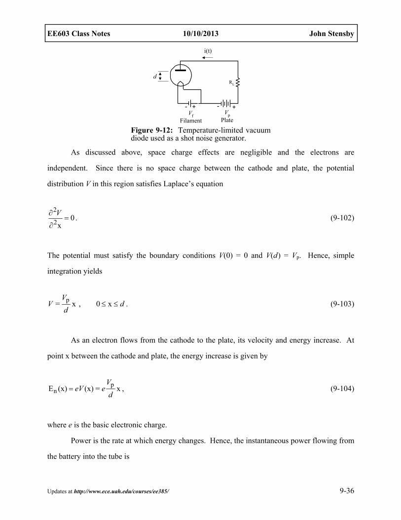
The basic circuit is illustrated by Figure 9-12. In a random manner, electrons are emitted

by the cathode, and they flow a distance d to the plate to form current i(t). If emitted at t = 0, an

independent electron contributes a current h(t), and the aggregate plate current is given by

kk

i(t) h(t t ) , (9-101)

where tk are the Poisson-distributed independent times at which electrons are emitted by the

cathode (see Equation (9-66)). In what follows, we approximate h(t).



As discussed above, space charge effects are negligible and the electrons are

independent. Since there is no space charge between the cathode and plate, the potential

distribution V in this region satisfies Laplace’s equation

2

20

x

V. (9-102)

The potential must satisfy the boundary conditions V(0) = 0 and V(d) = Vp. Hence, simple

integration yields

p= x , 0 x

VV d

d. (9-103)

As an electron flows from the cathode to the plate, its velocity and energy increase. At

point x between the cathode and plate, the energy increase is given by

pnE (x) (x) = x

VeV e

d, (9-104)

where e is the basic electronic charge.

Power is the rate at which energy changes. Hence, the instantaneous power flowing from

the battery into the tube is

RL

+-+-

i(t)

VpPlate

VfFilament

d

Figure 9-12: Temperature-limited vacuum diode used as a shot noise generator.



pn np

dE dE dx dxh

dt dx dt dt

Ve V

d, (9-105)

where h(t) is current due to the flow of a single electron (note that d -1dx/dt has units of sec-1 so

that (e/d ) dx/dt has units of charge/sec, or current). Equation (9-105) can be solved for current to

obtain

xd

h vdt

e x e

d d, (9-106)

where vx is the instantaneous velocity of the electron.

Electron velocity can be found by applying Newton’s laws. The force on an electron is

just e(Vp/d), the product of electronic charge and electric field strength. Since force is equal to

the product of electron mass m and acceleration ax, we have

xa =pVe

m d. (9-107)

As it is emitted by the cathode, an electron has an initial velocity that is Maxwellian distributed.

However, to simplify this example we will assume that the initial velocity is zero. With this

assumption, electron velocity can be obtained by integrating (9-107) to obtain

xv = tpVe

m d. (9-108)

Over transition time tT the average velocity is

x x0

1v v dt =

2 Tt p

TT T

Ve dt

t m d t. (9-109)



Finally, combine these last two equations to obtain

x 22

v = t, 0 t

T

Td

tt

. (9-110)

With the aid of this last relationship, we can determine current as a function of time.

Simply combine (9-106) and (9-110) to obtain

22

h(t) t, 0 t

TT

et

t, (9-111)

the current pulse generated by a single electron as it travels from the cathode to the plate. This

current pulse is depicted by Figure 9-13.

The bandwidth of shot noise s(t) is of interest. For example, we may use the noise

generator to make relative measurements on a communication receiver, and we may require the

noise spectrum to be “flat” (or “white”) over the receiver bandwidth (the noise spectrum

amplitude is not important since we are making relative measurements). To a certain “flatness”,

we can compute and examine the power spectrum of standardized s(t) described by (9-90). As

given by (9-91), the autocorrelation of s(t) is

t

h(t)

tT

2e/tT

Figure 9-13: Current due to a single electron emitted by the cathode at t = 0.



2 22

0

4R ( ) 2 t(t + )dt = 1 1 , 0

3 2

R ( ), 0

0, otherwise

Tt

s TT T T T

s T

e et

t t t t

t . (9-112)

The power spectrum of s(t) is the Fourier transform of (9-112), a result given by

2s 40

4( ) 2 R ( ) cos( )d ( ) 2(1 cos sin )

( )

T T T TT

S t t t tt

. (9-113)

Plots of the autocorrelation and relative power spectrum (plotted in dB relative to peak power at

= 0) are given by Figures 9-14 and 9-15, respectively.

To within 3dB, the power spectrum is “flat” from DC to a little over = /tT. For the

Sylvania 5722 noise generator diode, the cathode-to-plate spacing is .0375 inches and the transit

time is about 310-10 seconds. For this diode, the 3dB cutoff would be about 1/2tT = 1600Mhz.

In practical application, where electrode/circuit stray capacitance/inductance limits frequency

range, the Sylvania 5722 has been used in commercial noise generators operating at over

400Mhz.

Rs()

24

3 T

e

t

tT-tT Figure 9-14: Autocorrelation function of normalized shot noise process.

-10

-8

-6

-4

-2

2

Rel

ativ

e P

ower

(dB

)

(Rad/Sec)/tT

10Log{S()/S(0)}

0

Figure 9-15: Relative power spectrum of nor-malized shot noise process.

Documents

EE603 Class Notes 10/10/2013 John Stensby Chapter 9 ... · EE603 Class Notes 10/10/2013 John Stensby Updates at 9-1 Chapter 9: Commonly Used Models: Narrow-Band Gaussian Noise and