EECC756 - Shaaban #1 lec # 8 Spring2001 4-9-2001 Synchronous Iteration Iteration-based computation is a powerful method for solving numerical (and some

EECC756 - ShaabanEECC756 - Shaaban#1 lec # 8 Spring2001 4-9-2001

Synchronous IterationSynchronous Iteration• Iteration-based computation is a powerful method for solving

numerical (and some non-numerical) problems.

• For numerical problems, a calculation is repeated and each time, a result is obtained which is used on the next execution. The process is repeated until the desired results are obtained.

• Though iterative methods are is sequential in nature, parallel implementation can be successfully employed when there are multiple independent instances of the iteration. In some cases this is part of the problem specification and sometimes one must rearrange the problem to obtain multiple independent instances.

• The term "synchronous iteration" is used to describe solving a problem by iteration where different tasks may be performing separate iterations but the iterations must be synchronized using point-to-point synchronization, barriers, or other synchronization mechanisms.


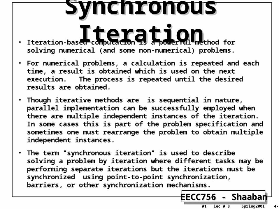
BarriersBarriersA synchronization mechanism

applicable to shared-memory

as well as message-passing,

where each process must wait

until all members of a specific

process group reach a specific

reference point in their

computation

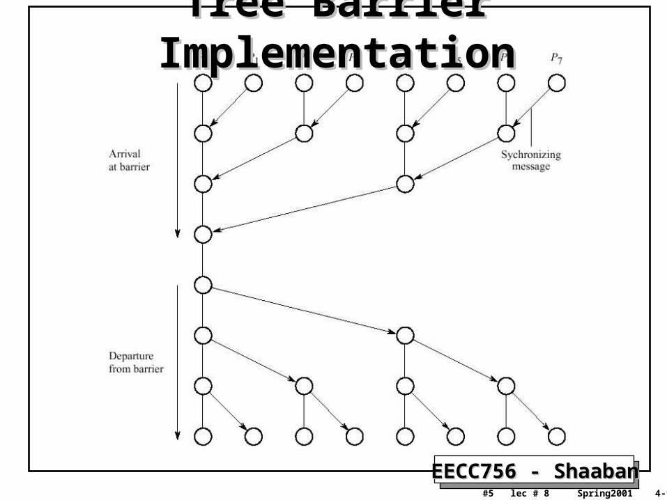
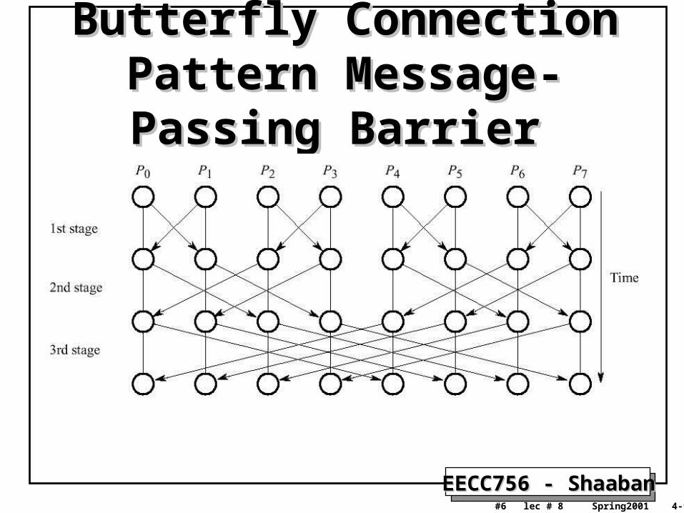
• Possible Implementations:– A library call possibly implemented using a counter– Using individual point-to-point synchronization forming:

• A tree• Butterfly connection pattern.


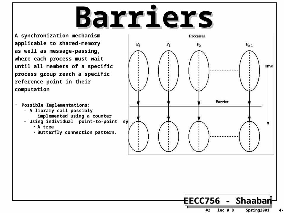
Processes Reaching A Barrier Processes Reaching A Barrier At Different TimesAt Different Times


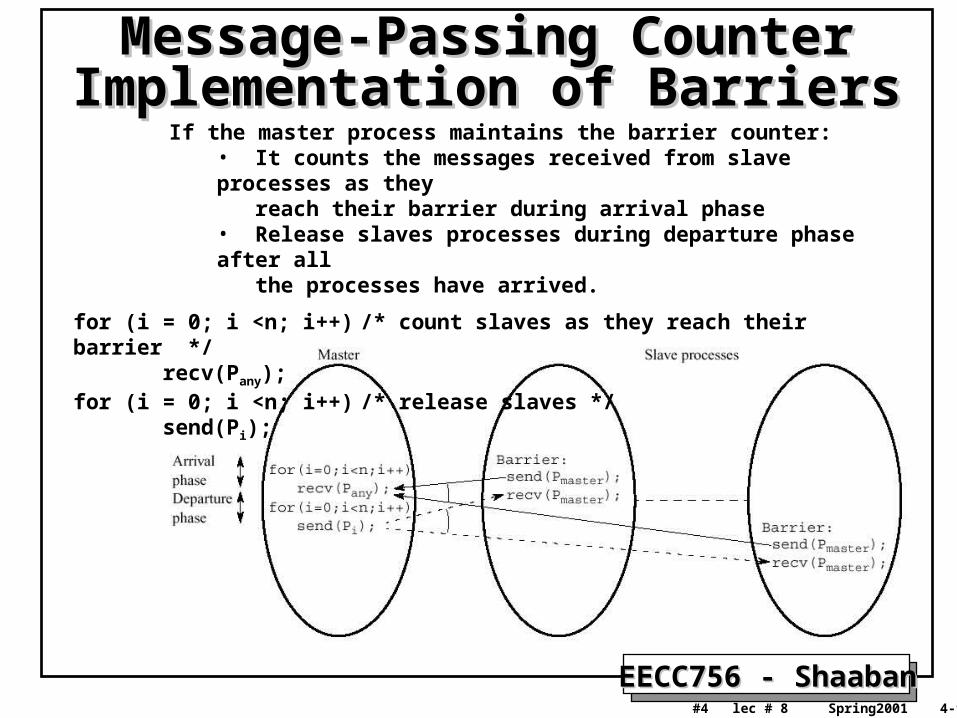
Message-Passing Counter Message-Passing Counter Implementation of BarriersImplementation of Barriers If the master process maintains the barrier counter:

• It counts the messages received from slave processes as they reach their barrier during arrival phase• Release slaves processes during departure phase after all the processes have arrived.

for (i = 0; i <n; i++) /* count slaves as they reach their barrier */ recv(Pany);for (i = 0; i <n; i++) /* release slaves */ send(Pi);


Tree Barrier ImplementationTree Barrier Implementation


Butterfly Connection Pattern Butterfly Connection Pattern Message-Passing BarrierMessage-Passing Barrier


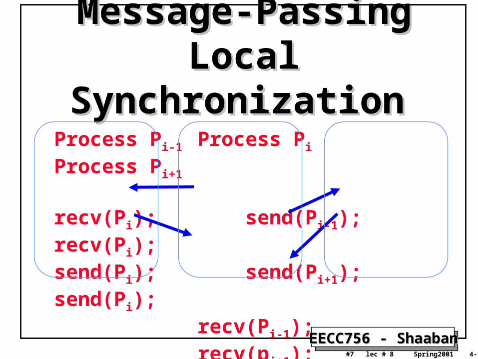
Message-Passing Local Message-Passing Local SynchronizationSynchronization

Process Pi-1Process Pi Process Pi+1

recv(Pi); send(Pi-1); recv(Pi);send(Pi); send(Pi+1); send(Pi);

recv(Pi-1);recv(pi+1);


Synchronous Iteration Program Example:Synchronous Iteration Program Example:

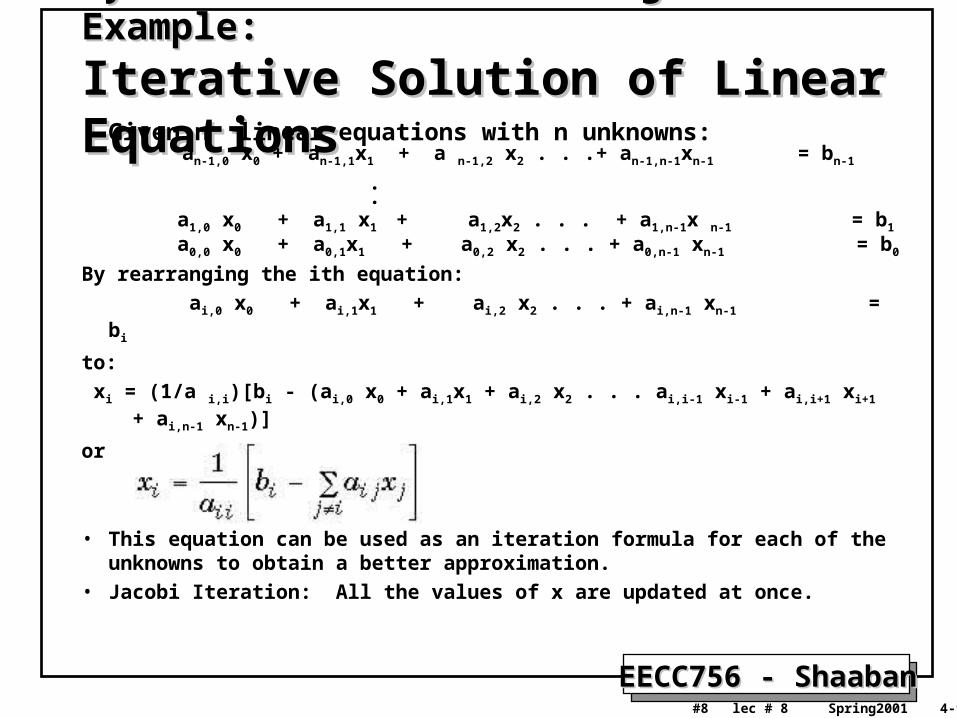
Iterative Solution of Linear EquationsIterative Solution of Linear Equations• Given n linear equations with n unknowns: an-1,0 x0 + an-1,1x1 + a n-1,2 x2 . . .+ an-1,n-1xn-1 = bn-1 . . a1,0 x0 + a1,1 x1 + a1,2x2 . . . + a1,n-1x n-1 = b1

a0,0 x0 + a0,1x1 + a0,2 x2 . . . + a0,n-1 xn-1 = b0

By rearranging the ith equation:

ai,0 x0 + ai,1x1 + ai,2 x2 . . . + ai,n-1 xn-1 = bi

to:

xi = (1/a i,i)[bi - (ai,0 x0 + ai,1x1 + ai,2 x2 . . . ai,i-1 xi-1 + ai,i+1 xi+1 + ai,n-1 xn-1)]

or

• This equation can be used as an iteration formula for each of the unknowns to obtain a better approximation.

• Jacobi Iteration: All the values of x are updated at once.


Iterative Solution of Linear EquationsIterative Solution of Linear Equations

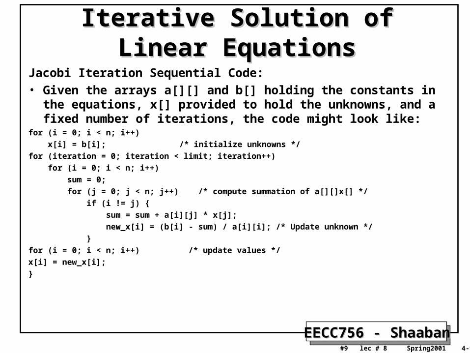
Jacobi Iteration Sequential Code: • Given the arrays a[][] and b[] holding the constants in the equations, x[]

provided to hold the unknowns, and a fixed number of iterations, the code might look like:

for (i = 0; i < n; i++)

x[i] = b[i]; /* initialize unknowns */

for (iteration = 0; iteration < limit; iteration++)

for (i = 0; i < n; i++)

sum = 0;

for (j = 0; j < n; j++) /* compute summation of a[][]x[] */

if (i != j) {

sum = sum + a[i][j] * x[j];

new_x[i] = (b[i] - sum) / a[i][i]; /* Update unknown */

}

for (i = 0; i < n; i++) /* update values */

x[i] = new_x[i];

}


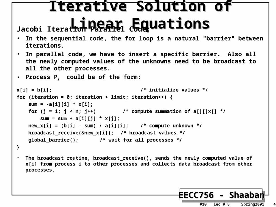
Iterative Solution of Linear EquationsIterative Solution of Linear EquationsJacobi Iteration Parallel Code: • In the sequential code, the for loop is a natural "barrier" between iterations.

• In parallel code, we have to insert a specific barrier. Also all the newly computed values of the unknowns need to be broadcast to all the other processes.

• Process Pi could be of the form:

x[i] = b[i]; /* initialize values */

for (iteration = 0; iteration < limit; iteration++) {

sum = -a[i][i] * x[i];

for (j = 1; j < n; j++) /* compute summation of a[][]x[] */

sum = sum + a[i][j] * x[j];

new_x[i] = (b[i] - sum) / a[i][i]; /* compute unknown */

broadcast_receive(&new_x[i]); /* broadcast values */

global_barrier(); /* wait for all processes */

}

• The broadcast routine, broadcast_receive(), sends the newly computed value of x[i] from process i to other processes and collects data broadcast from other processes.


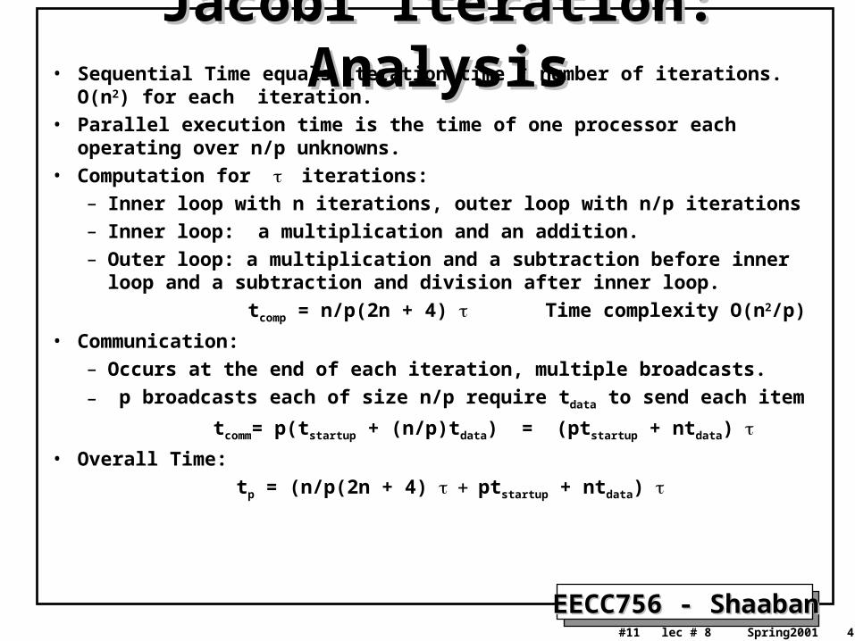
Jacobi Iteration: AnalysisJacobi Iteration: Analysis• Sequential Time equals iteration time * number of iterations. O(n2) for each

iteration.

• Parallel execution time is the time of one processor each operating over n/p unknowns.

• Computation for iterations:

– Inner loop with n iterations, outer loop with n/p iterations

– Inner loop: a multiplication and an addition.

– Outer loop: a multiplication and a subtraction before inner loop and a subtraction and division after inner loop.

tcomp = n/p(2n + 4) Time complexity O(n2/p)

• Communication:

– Occurs at the end of each iteration, multiple broadcasts.

– p broadcasts each of size n/p require tdata to send each item

tcomm= p(tstartup + (n/p)tdata) = (ptstartup + ntdata)

• Overall Time:

tp = (n/p(2n + 4) ptstartup + ntdata)


Effects of Computation And Effects of Computation And Communication in Jacobi IterationCommunication in Jacobi Iteration

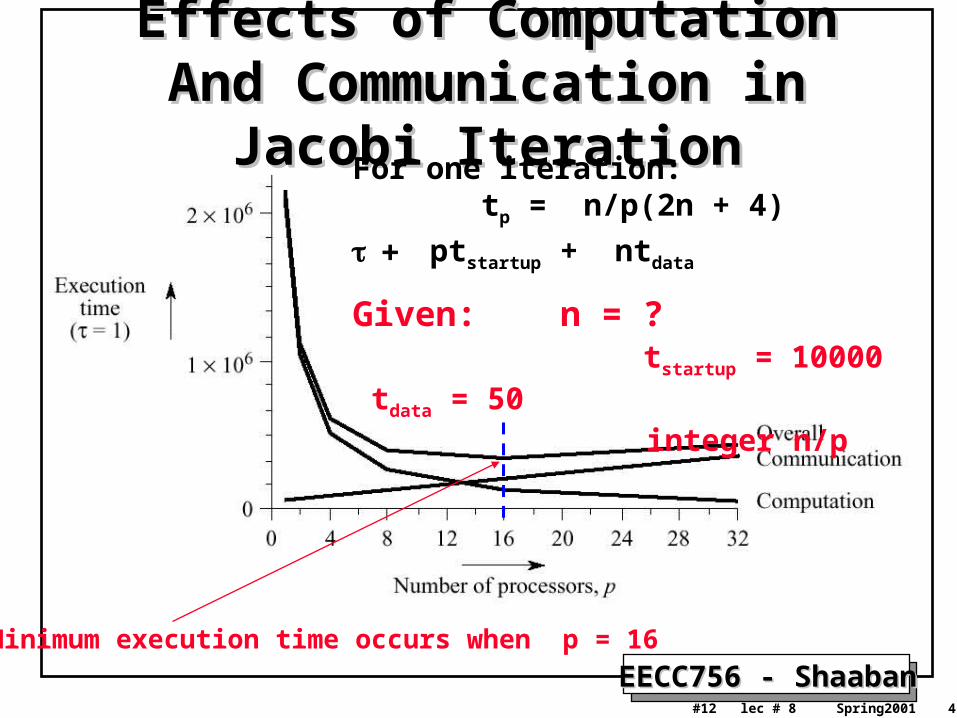
For one iteration: tp = n/p(2n + 4) ptstartup + ntdata

Given: n = ? tstartup = 10000 tdata = 50 integer n/p

Minimum execution time occurs when p = 16


Dynamic Load BalancingDynamic Load Balancing• To achieve best performance of a parallel computing system running

a parallel problem, it’s essential to maximize processor utilization by distributing the computation load evenly or balancing the load among the available processors.

• Optimal static load balancing, optimal mapping or scheduling, is an intractable NP-complete problem, except for specific problems on specific networks.

• Hence heuristics are usually used to select processors for processes.

• Even the best static mapping may offer the best execution time due to changing conditions at runtime and the process may need to done dynamically.

• The methods used for balancing the computational load dynamically

among processors can be broadly classified as:

1. Centralized dynamic load balancing.

2. Decentralized dynamic load balancing.


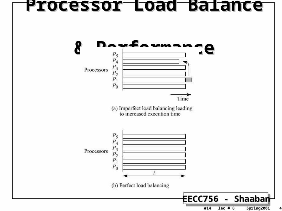
Processor Load Balance Processor Load Balance & Performance& Performance


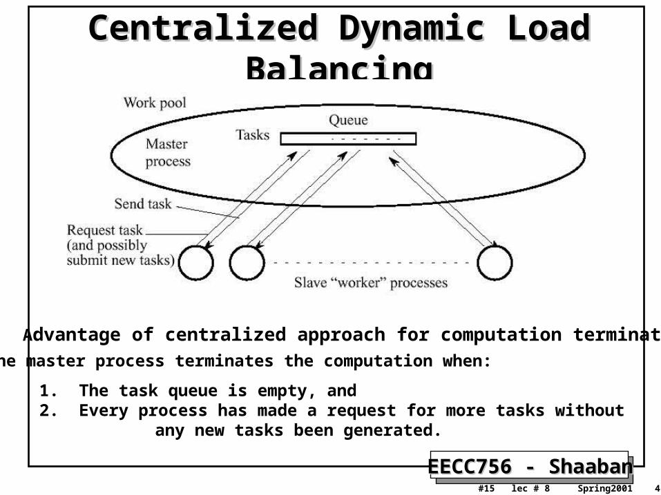
Centralized Dynamic Load BalancingCentralized Dynamic Load Balancing

Advantage of centralized approach for computation termination:

The master process terminates the computation when:

1. The task queue is empty, and 2. Every process has made a request for more tasks without any new tasks been generated.


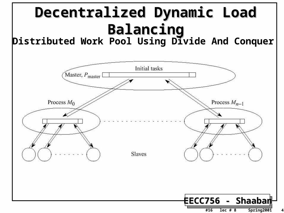
Decentralized Dynamic Load BalancingDecentralized Dynamic Load BalancingDistributed Work Pool Using Divide And Conquer


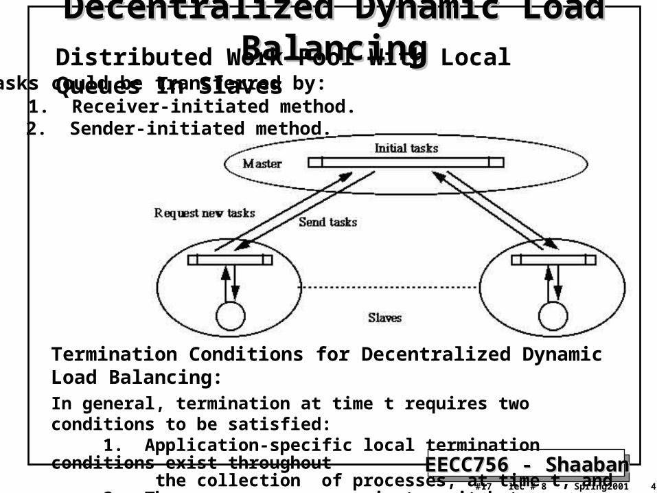
Decentralized Dynamic Load Decentralized Dynamic Load BalancingBalancingDistributed Work Pool With Local Queues In Slaves

Termination Conditions for Decentralized Dynamic Load Balancing:

In general, termination at time t requires two conditions to be satisfied: 1. Application-specific local termination conditions exist throughout the collection of processes, at time t, and 2. There are no messages in transit between processes at time t.

Tasks could be transferred by: 1. Receiver-initiated method. 2. Sender-initiated method.


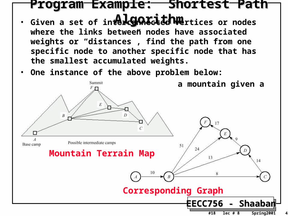
Program Example: Shortest Path AlgorithmProgram Example: Shortest Path Algorithm• Given a set of interconnected vertices or nodes where the links

between nodes have associated weights or “distances”, find the path from one specific node to another specific node that has the smallest accumulated weights.

• One instance of the above problem below:

– “Find the best way to climb a mountain given a terrain map.”

Mountain Terrain Map

Corresponding Graph


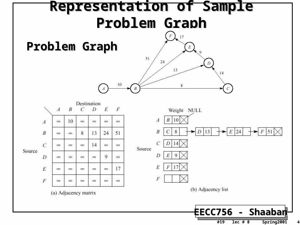
Representation of Sample Problem GraphRepresentation of Sample Problem Graph

Problem GraphProblem Graph


Moore’s Single-source Moore’s Single-source Shortest-path AlgorithmShortest-path Algorithm

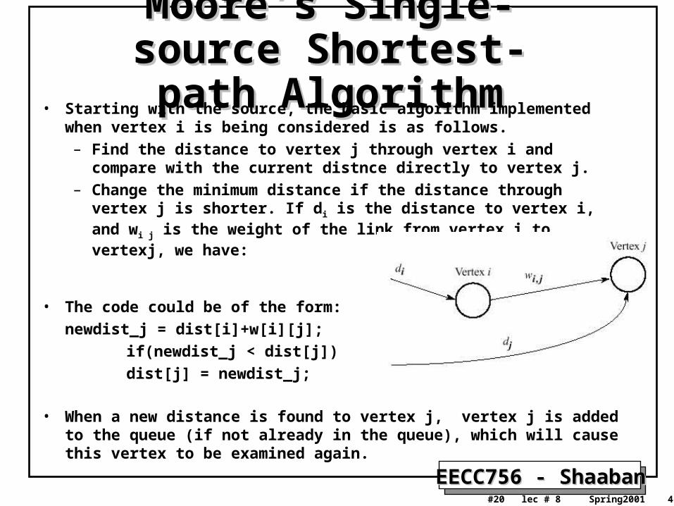
• Starting with the source, the basic algorithm implemented when vertex i is being considered is as follows.

– Find the distance to vertex j through vertex i and compare with the current distnce directly to vertex j.

– Change the minimum distance if the distance through vertex j is shorter. If di is the distance to vertex i, and wi j is the weight of the link from vertex i to vertexj, we have:

dj = min(dj, di+wi j)

• The code could be of the form:

newdist_j = dist[i]+w[i][j];

if(newdist_j < dist[j])

dist[j] = newdist_j;

• When a new distance is found to vertex j, vertex j is added to the queue (if not already in the queue), which will cause this vertex to be examined again.


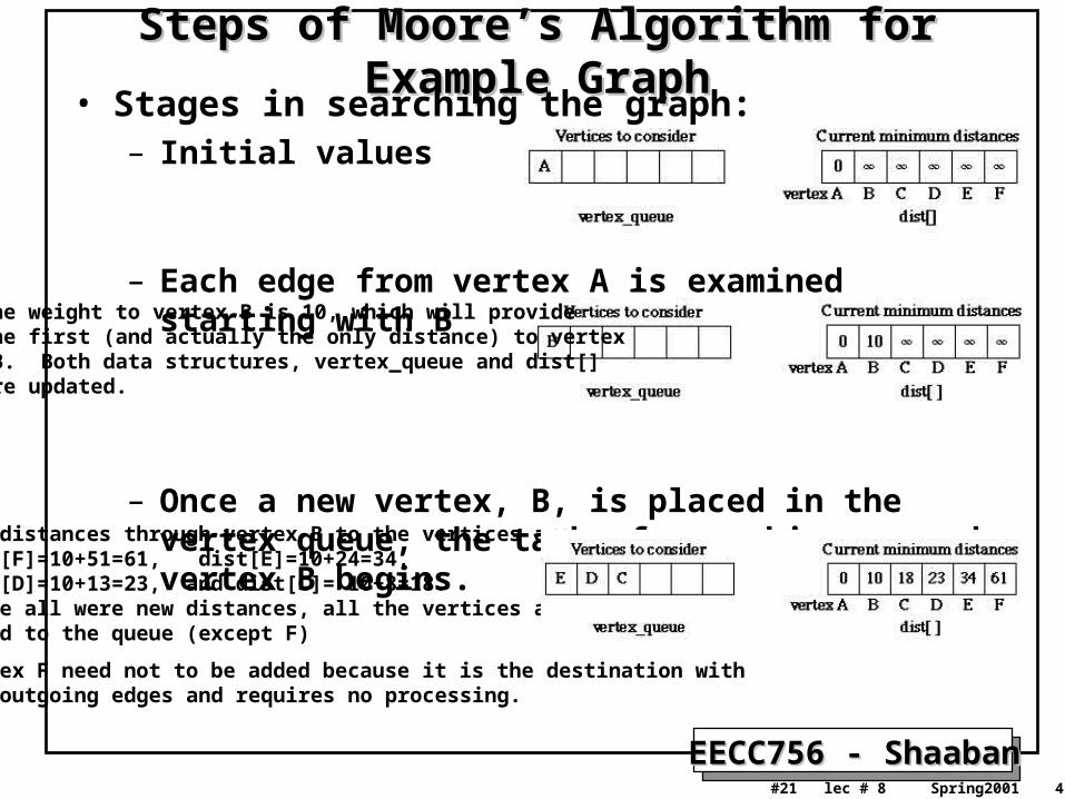
Steps of Moore’s Algorithm for Example GraphSteps of Moore’s Algorithm for Example Graph• Stages in searching the graph:

– Initial values

– Each edge from vertex A is examined starting with B

– Once a new vertex, B, is placed in the vertex queue, the task of searching around vertex B begins.

The weight to vertex B is 10, which will provide the first (and actually the only distance) to vertex B. Both data structures, vertex_queue and dist[] are updated.

The distances through vertex B to the vertices aredist[F]=10+51=61, dist[E]=10+24=34, dist[D]=10+13=23, and dist[C]= 10+8=18. Since all were new distances, all the vertices are added to the queue (except F)

Vertex F need not to be added because it is the destination with no outgoing edges and requires no processing.


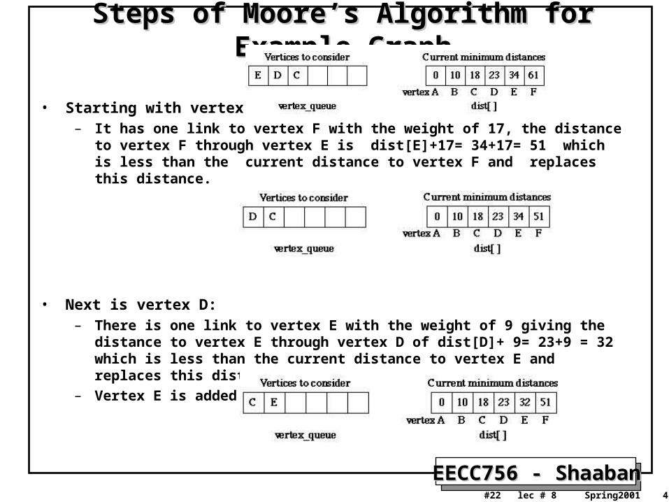
• Starting with vertex E: – It has one link to vertex F with the weight of 17, the distance to vertex F through vertex E

is dist[E]+17= 34+17= 51 which is less than the current distance to vertex F and replaces this distance.

• Next is vertex D:– There is one link to vertex E with the weight of 9 giving the distance to vertex E through

vertex D of dist[D]+ 9= 23+9 = 32 which is less than the current distance to vertex E and replaces this distance.

– Vertex E is added to the queue.

Steps of Moore’s Algorithm for Example GraphSteps of Moore’s Algorithm for Example Graph


Steps of Moore’s Algorithm for Example GraphSteps of Moore’s Algorithm for Example Graph

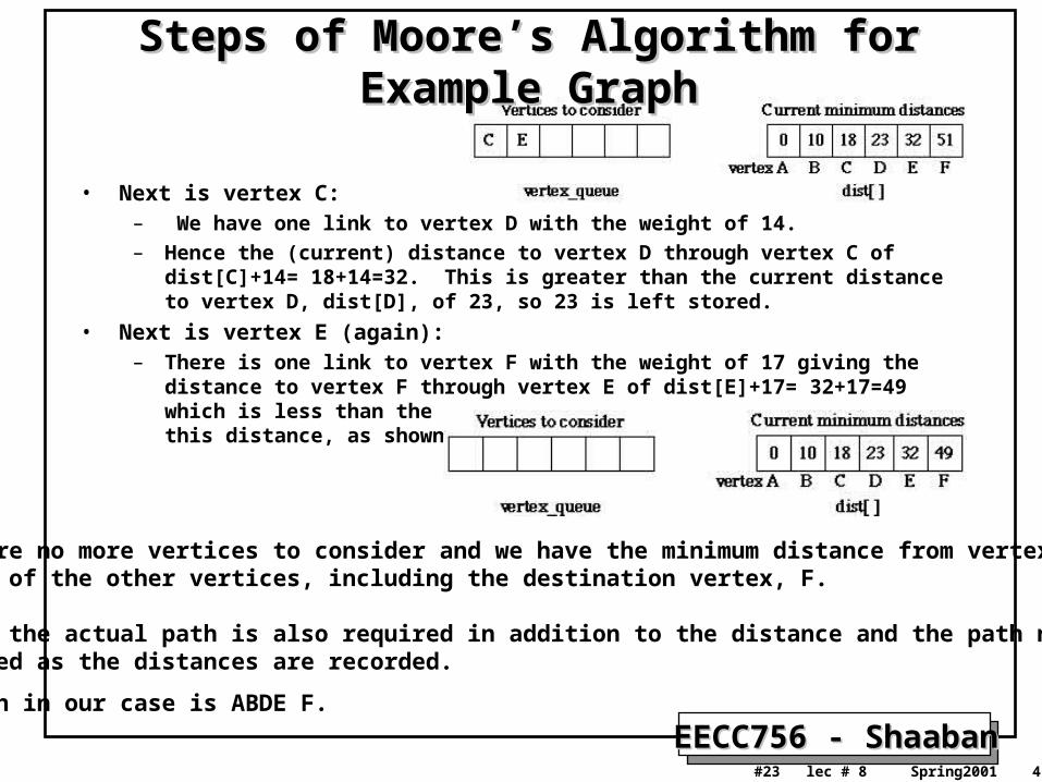
• Next is vertex C:– We have one link to vertex D with the weight of 14.

– Hence the (current) distance to vertex D through vertex C of dist[C]+14= 18+14=32. This is greater than the current distance to vertex D, dist[D], of 23, so 23 is left stored.

• Next is vertex E (again):– There is one link to vertex F with the weight of 17 giving the distance to vertex F through

vertex E of dist[E]+17= 32+17=49 which is less than the current distance to vertex F and replaces this distance, as shown below:

There are no more vertices to consider and we have the minimum distance from vertex A to each of the other vertices, including the destination vertex, F.

Usually the actual path is also required in addition to the distance and the path needs tobe stored as the distances are recorded.

The path in our case is ABDE F.


Moore’s Single-source Shortest-path AlgorithmMoore’s Single-source Shortest-path Algorithm

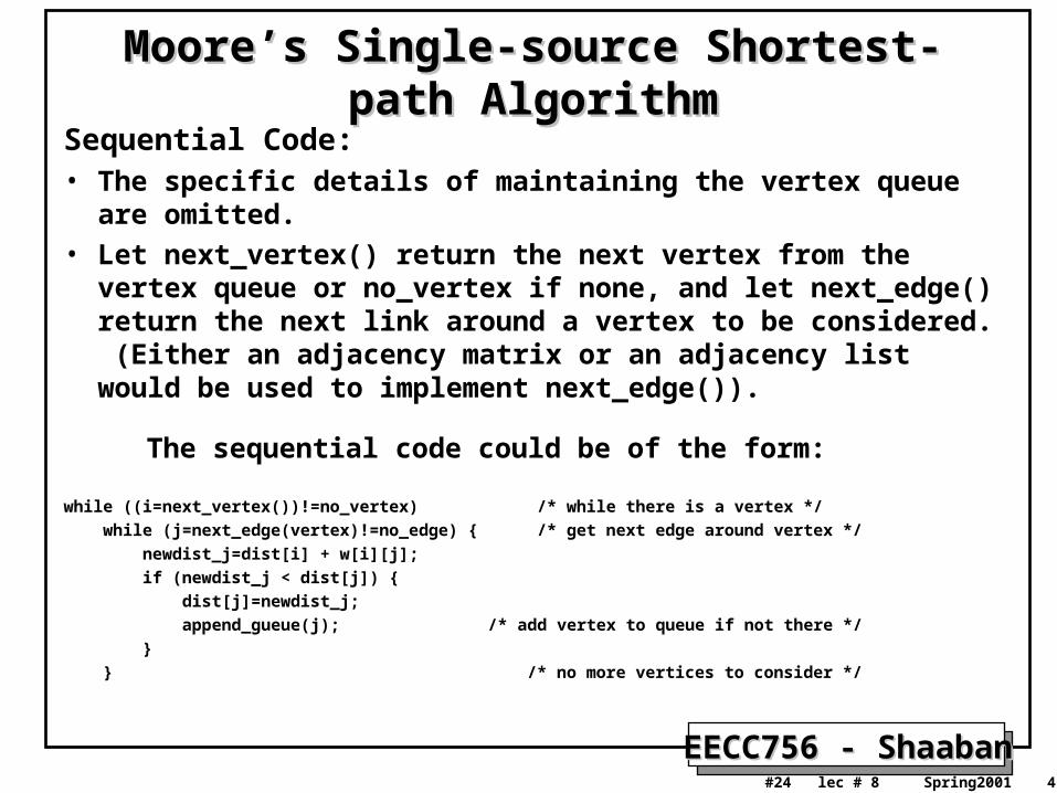
Sequential Code: • The specific details of maintaining the vertex queue are omitted.

• Let next_vertex() return the next vertex from the vertex queue or no_vertex if none, and let next_edge() return the next link around a vertex to be considered. (Either an adjacency matrix or an adjacency list would be used to implement next_edge()).

The sequential code could be of the form:

while ((i=next_vertex())!=no_vertex) /* while there is a vertex */

while (j=next_edge(vertex)!=no_edge) { /* get next edge around vertex */

newdist_j=dist[i] + w[i][j];

if (newdist_j < dist[j]) {

dist[j]=newdist_j;

append_gueue(j); /* add vertex to queue if not there */

}

} /* no more vertices to consider */


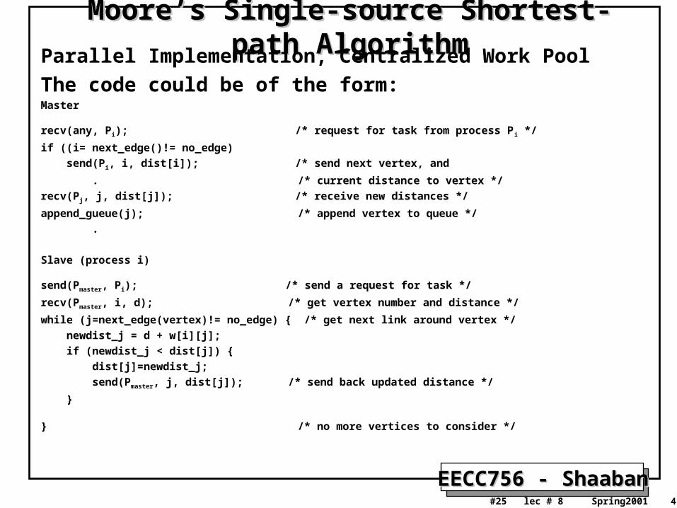
Moore’s Single-source Shortest-path AlgorithmMoore’s Single-source Shortest-path AlgorithmParallel Implementation, Centralized Work Pool

The code could be of the form: Master

recv(any, Pi); /* request for task from process Pi */

if ((i= next_edge()!= no_edge)

send(Pi, i, dist[i]); /* send next vertex, and

. /* current distance to vertex */

recv(Pj, j, dist[j]); /* receive new distances */

append_gueue(j); /* append vertex to queue */

.

Slave (process i)

send(Pmaster, Pi); /* send a request for task */

recv(Pmaster, i, d); /* get vertex number and distance */

while (j=next_edge(vertex)!= no_edge) { /* get next link around vertex */

newdist_j = d + w[i][j];

if (newdist_j < dist[j]) {

dist[j]=newdist_j;

send(Pmaster, j, dist[j]); /* send back updated distance */

}

} /* no more vertices to consider */


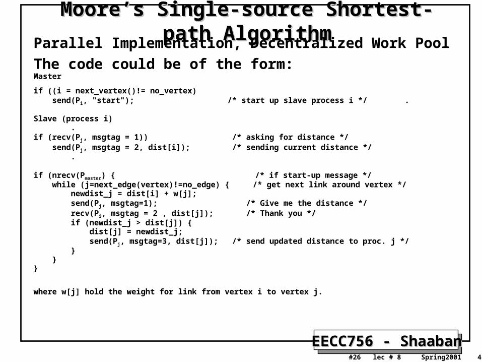
Moore’s Single-source Shortest-path AlgorithmMoore’s Single-source Shortest-path AlgorithmParallel Implementation, Decentralized Work Pool

The code could be of the form:Master

if ((i = next_vertex()!= no_vertex) send(Pi, "start"); /* start up slave process i */ . Slave (process i) .if (recv(Pj, msgtag = 1)) /* asking for distance */ send(Pj, msgtag = 2, dist[i]); /* sending current distance */ .

if (nrecv(Pmaster) { /* if start-up message */ while (j=next_edge(vertex)!=no_edge) { /* get next link around vertex */ newdist_j = dist[i] + w[j]; send(Pj, msgtag=1); /* Give me the distance */ recv(Pi, msgtag = 2 , dist[j]); /* Thank you */ if (newdist_j > dist[j]) { dist[j] = newdist_j; send(Pj, msgtag=3, dist[j]); /* send updated distance to proc. j */ } }}

where w[j] hold the weight for link from vertex i to vertex j.


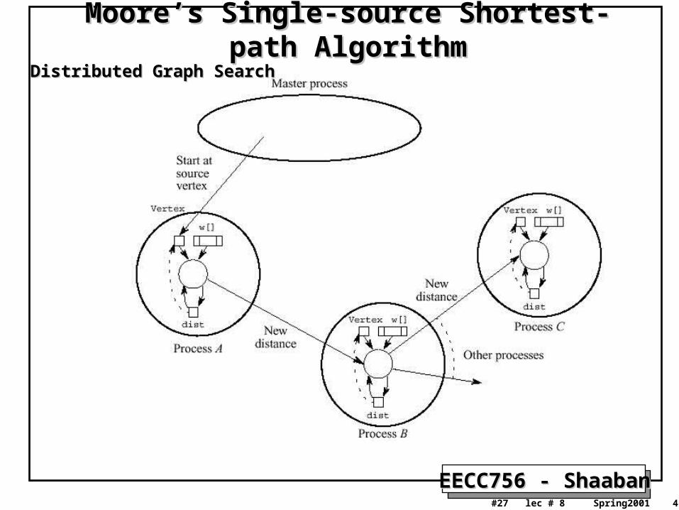
Moore’s Single-source Shortest-path AlgorithmMoore’s Single-source Shortest-path AlgorithmDistributed Graph SearchDistributed Graph Search

Documents

EECC756 - Shaaban #1 lec # 8 Spring2001 4-9-2001 Synchronous Iteration Iteration-based computation is a powerful method for solving numerical (and some