EECS 16B: FALL 2015 – MIDTERM 1 1/14

University of California College of Engineering

Department of Electrical Engineering and Computer Sciences

E. Alon, B. Ayazifar, C. Tomlin Thurs., Nov. 19, 2015 G. Ranade 11:00-12:30pm

EECS 16B: FALL 2015—MIDTERM 2

Important notes: Please read every question carefully and completely – the setup may or may not be the same as what you have seen before. Also, be sure to show your work since that is the only way we can potentially give you partial credit.

Problem 1: _____/ 18

Problem 2: _____/ 26

Problem 3: _____/ 22

Total: _____/ 66

NAME Last First

SID

Login

EECS 16B: FALL 2015 – MIDTERM 1 2/14

PROBLEM 1. Miscellaneous (18 points)

a) (6 pts) Assuming that for every inverter in the chain shown below, Ron,n = Ron,p = 1kΩ, and Cg,n = Cg,p = 20fF, what is the delay from Vin transitioning from 0V to Vdd to Vout transitioning from Vdd to 0V?

Vin40fF

Out+-

+-

EECS 16B: FALL 2015 – MIDTERM 1 3/14

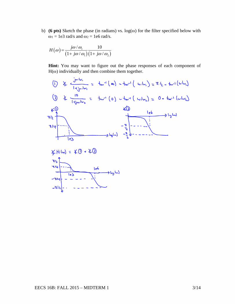
b) (6 pts) Sketch the phase (in radians) vs. log(ω) for the filter specified below with ω1 = 1e3 rad/s and ω2 = 1e6 rad/s.

( ) ( ) ( )1

1 2

/ 101 / 1 /

jHj jω ωωω ω ω ω

=+ +

Hint: You may want to figure out the phase responses of each component of H(ω) individually and then combine them together.

EECS 16B: FALL 2015 – MIDTERM 1 4/14

c) (6 pts) It turns out that filters can be realized not only be electrical components like we have seen so far in class, but out of mechanical (and even electro-mechanical) components as well. The differential equation provided below represents the relationship between an applied force F(t) (that could be coming from for example an incoming audio signal) and the displacement x(t) of a mass connected to a spring and damper; m is the mass, b is the damping coefficient, and k is the spring constant. If we define H(ω) = x(t) / F(t) for a sinusoidal F(t), derive H(ω) for this mechanical filter.

2

2

( ) ( )b ( ) 0d x t dx tm kx t F(t)dt dt

+ + − =

EECS 16B: FALL 2015 – MIDTERM 1 5/14

PROBLEM 2. Underwater Communications (26 pts) Communicating underwater can be very challenging for a number of reasons, and one of the techniques adopted by submarines is to use subsonic signals – that is, very low frequencies – for communication. In this problem we’ll explore the design of such a communication system for an underwater autonomous robot called FiShT33n. Important Note: This problem has many sub-parts, but it has been set up in a way that you can complete each sub-part without having gotten the (correct) answer to the previous parts.

a) (2 pts) For our initial design, let’s assume that FiShT33n communicates by sending signals that can have frequency components anywhere between -15Hz and 15Hz (i.e., the bandwidth is 30Hz, centered at 0Hz), and that the measured frequency of the signal is used to convey the desired command or message. Given these specifications, what is the minimum frequency that FiShT33n should use to sample the received signal? (As additional clarification and an example of how the communication works, if the robot’s human monitor sends a signal x(t) = cos(2*π*10Hz*t) and FiShT33n sees that it is receiving a signal whose frequency corresponds to 10Hz, that would mean “stop and search this area”. Similarly, if the monitor sends a signal x(t) = cos(2*π*5Hz*t) and FiShT33n receives a signal whose frequency corresponds to 5Hz, that would mean “get away – a shark is about to try and eat you”.)

EECS 16B: FALL 2015 – MIDTERM 1 6/14

b) (4 pts) Let’s assume that your answer to part (a) was 40Hz, that you chose to have FiShT33n’s receiver sample at this frequency in order to save power, and that you tried to save some money by not put any filtering in front of the receiver. After some initial failed experiments with FiShT33n out in the ocean, you realize that the robot is sometimes getting confused by the presence of audio signals from things like dolphins, whales, humans, and boats, and that these signals are all at frequencies of 400Hz and above. Assuming that all interfering signals are at a frequency of exactly 410Hz, after sampling, what continuous-time frequency would FiShT33n’s receiver perceive the interfering signal as being equivalent to?

EECS 16B: FALL 2015 – MIDTERM 1 7/14

c) (6 pts) Continuing to assume that FiShT33n samples the received signal at 40Hz and that external interference is always at frequencies of 400Hz and above, select a value for ωc so that the H(ω) provided below attenuates the interfering signals by at least a factor of 50 while attenuating the desired signal by at most 10%. (In other words, ||H(ω)|| < 1/50 for frequencies associated with the interference, while for frequencies associated with the signal ||H(ω)|| > 0.9.)

( )( )2

11 / c

Hj

ωω ω

=+

EECS 16B: FALL 2015 – MIDTERM 1 8/14

d) (6 pts) Assuming that your answer to part (c) was ωc = 2π∗100Hz, design an analog circuit that realizes this H(ω). You can use any combination of op-amps and passive components to implement this circuit, but be sure to label the values of any of these passive components.

EECS 16B: FALL 2015 – MIDTERM 1 9/14

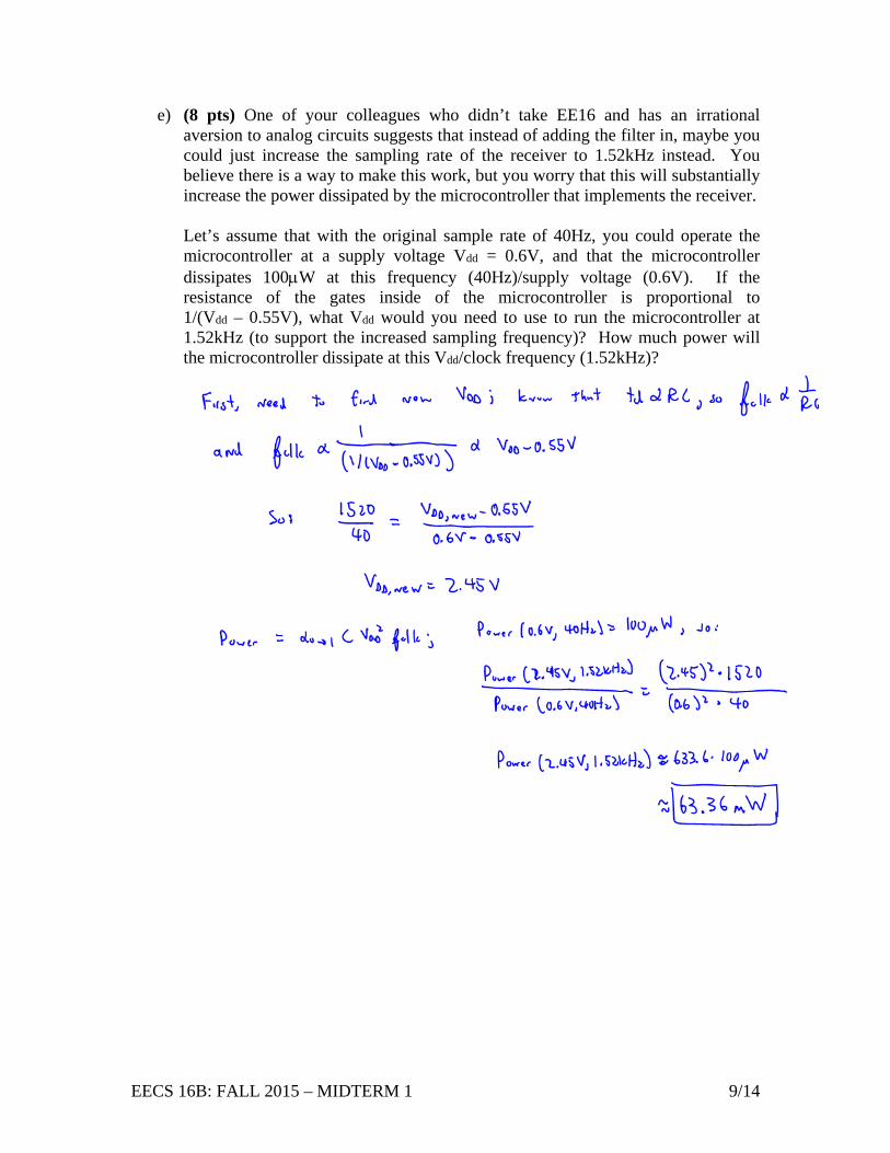
e) (8 pts) One of your colleagues who didn’t take EE16 and has an irrational aversion to analog circuits suggests that instead of adding the filter in, maybe you could just increase the sampling rate of the receiver to 1.52kHz instead. You believe there is a way to make this work, but you worry that this will substantially increase the power dissipated by the microcontroller that implements the receiver. Let’s assume that with the original sample rate of 40Hz, you could operate the microcontroller at a supply voltage Vdd = 0.6V, and that the microcontroller dissipates 100µW at this frequency (40Hz)/supply voltage (0.6V). If the resistance of the gates inside of the microcontroller is proportional to 1/(Vdd – 0.55V), what Vdd would you need to use to run the microcontroller at 1.52kHz (to support the increased sampling frequency)? How much power will the microcontroller dissipate at this Vdd/clock frequency (1.52kHz)?

EECS 16B: FALL 2015 – MIDTERM 1 10/14

PROBLEM 3. Controlling a Car (22 points) In this problem we will examine a simple model for a car driving on a road. The state of the car is x[k] = [z[k] v[k]]T, where z[k] is the position of the car at time kTs, v[k] is the velocity of the car at time kTs, and Ts is the sampling period. The car is driven by a force u[k] from its engine, which must counter a friction force Ff[k]. Finally, y[k] represents the variables that we will measure (sense). In this case, we can model the dynamics of the car as follows:

[ ][ ]

1

2

[ 1] [ ] ( [ ])

[ ]

0.1 0.01,

0 0.2

fx k Ax k B u k F k

y k Cx k

A Bλ

λ

+ = + −

=

= =

Note: for parts (a) through (c) of this problem, you can assume that the friction force Ff[k] = 0 for all k.

a) (4 pts) Let’s assume that C = 1 00 1

and that we want to set the velocity and

position to some desired values zd[k] and vd[k] by using closed-loop control with a forward gain matrix K = [k1 k2]. Provide expressions for the ACL and BCL matrices you would use to create a state-space model of the resulting closed-loop system.

EECS 16B: FALL 2015 – MIDTERM 1 11/14

b) (4 pts) Assuming that λ1 = 1 and λ2 = 2, derive the eigenvalues of ACL as a function of k1 and k2. Note: You do not need to actually solve for the eigenvalues – please just show the equation you would need to solve to find the eigenvalues.

EECS 16B: FALL 2015 – MIDTERM 1 12/14

c) (6 pts) Assuming that the eigenvalues of ACL are λ1 = (1-0.1*k1) and λ2 = (2-0.4k2+0.1*k12) (note that this may or may not be the correct answer to part (b)), explain whether you would choose to use a controller with K = [k1 k2] = [5 1] or K = [1 5]. You should be as clear and complete as possible in identifying the issues/tradeoffs when justifying your selection.

EECS 16B: FALL 2015 – MIDTERM 1 13/14

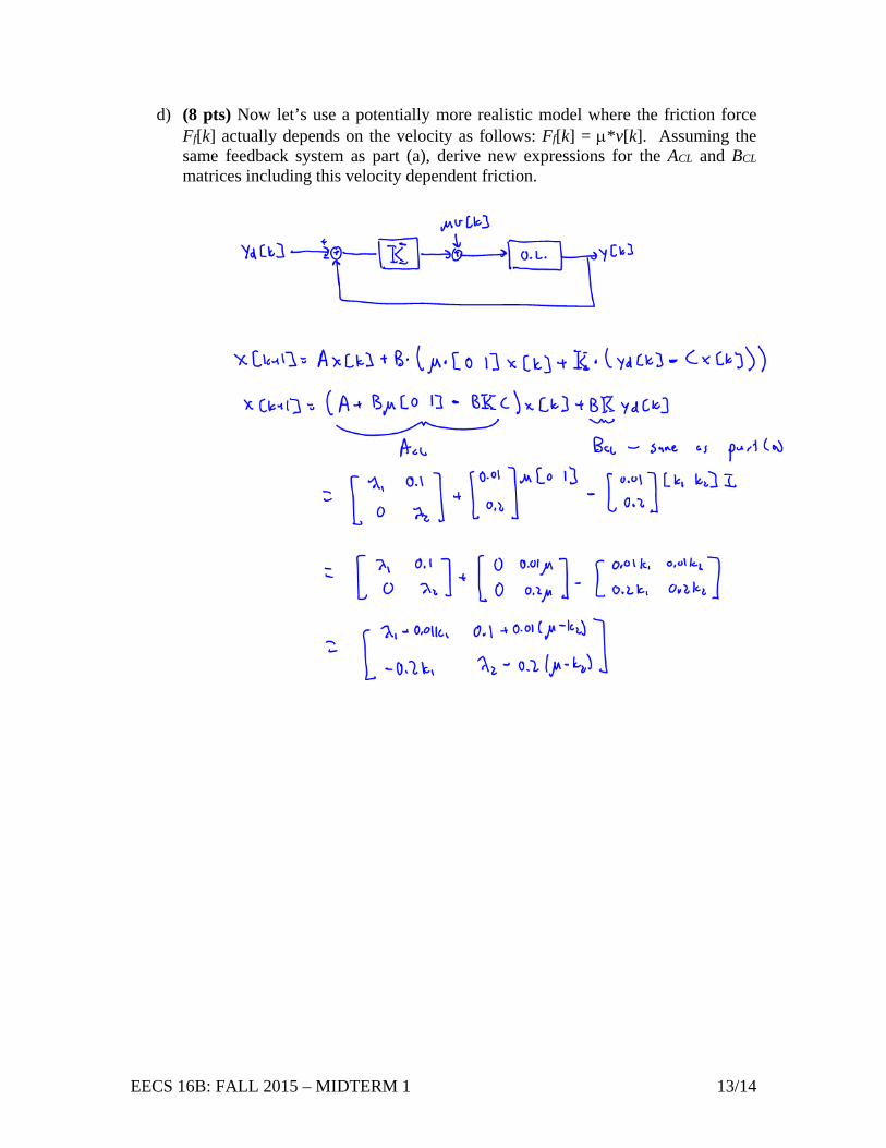
d) (8 pts) Now let’s use a potentially more realistic model where the friction force Ff[k] actually depends on the velocity as follows: Ff[k] = µ*v[k]. Assuming the same feedback system as part (a), derive new expressions for the ACL and BCL matrices including this velocity dependent friction.

EECS 16B: FALL 2015 – MIDTERM 1 14/14

e) (BONUS: 6 pts) Recall that the discrete-time state-space model we provided you for the car is actually the result of sampling the continuous-time inputs (in this case, position z(t) and velocity v(t)) going in to our sensors. Let’s assume that the road the car is driving on is rough in a way that the continuous time velocity is actually v(t) = vnom*[1+0.5*cos(2π*100Hz*t)] and that our sensor is sampling with Ts = 100ms. If the sensor directly samples v(t), as a function of vnom, what will the sensor’s output v[k] be? Assuming that we set vd[k] to a fixed constant value, what would this result (i.e., the relationship between vnom and v[k]) imply about the actual average velocity of the car?