Embed Size (px)
Citation preview

Effective Strong Dimension in Algorithmic Information
and Computational Complexity
Krishna B. Athreya 1 John M. Hitchcock 2 Jack H. Lutz 3
Elvira Mayordomo 4
1Departments of Mathematics and Statistics, Iowa State University, Ames, IA 50011, [email protected]. This research was supported in part by Air Force Office of Scientific Research GrantITSI F 49620-01-1-0076 and National Science Foundation grant 0344187.
2Department of Computer Science, University of Wyoming, Laramie, WY 82072, [email protected]. This research was supported in part by National Science Foundation grants 9988483and 0515313.
3Department of Computer Science, Iowa State University, Ames, IA 50011, USA. [email protected] research was supported in part by National Science Foundation grants 9988483 and 0344187, and bySpanish Government MEC project TIN 2005-08832-C03-02.
4Departamento de Informatica e Ingenierıa de Sistemas, Universidad de Zaragoza, 50015 Zaragoza,SPAIN. elvira at unizar dot es. This research was supported in part by Spanish Government MECprojects TIC2002-04019-C03-03 and TIN 2005-08832-C03-02, and by National Science Foundation grants9988483 and 0344187. It was done while visiting Iowa State University.
Abstract
The two most important notions of fractal dimension are Hausdorff dimension, developed by Haus-dorff (1919), and packing dimension, developed independently by Tricot (1982) and Sullivan (1984).Both dimensions have the mathematical advantage of being defined from measures, and both haveyielded extensive applications in fractal geometry and dynamical systems.
Lutz (2000) has recently proven a simple characterization of Hausdorff dimension in terms ofgales, which are betting strategies that generalize martingales. Imposing various computabilityand complexity constraints on these gales produces a spectrum of effective versions of Hausdorffdimension, including constructive, computable, polynomial-space, polynomial-time, and finite-statedimensions. Work by several investigators has already used these effective dimensions to shedsignificant new light on a variety of topics in theoretical computer science.
In this paper we show that packing dimension can also be characterized in terms of gales.Moreover, even though the usual definition of packing dimension is considerably more complexthan that of Hausdorff dimension, our gale characterization of packing dimension is an exact dualof – and every bit as simple as – the gale characterization of Hausdorff dimension.
Effectivizing our gale characterization of packing dimension produces a variety of effective strongdimensions, which are exact duals of the effective dimensions mentioned above. In general (and inanalogy with the classical fractal dimensions), the effective strong dimension of a set or sequence isat least as great as its effective dimension, with equality for sets or sequences that are sufficientlyregular.
We develop the basic properties of effective strong dimensions and prove a number of resultsrelating them to fundamental aspects of randomness, Kolmogorov complexity, prediction, Booleancircuit-size complexity, polynomial-time degrees, and data compression. Aside from the abovecharacterization of packing dimension, our two main theorems are the following.
1. If ~β = (β0, β1, . . .) is a computable sequence of biases that are bounded away from 0 and R israndom with respect to ~β, then the dimension and strong dimension of R are the lower andupper average entropies, respectively, of ~β.
2. For each pair of ∆02-computable real numbers 0 < α ≤ β ≤ 1, there exists A ∈ E such that
the polynomial-time many-one degree of A has dimension α in E and strong dimension β inE.
Our proofs of these theorems use a new large deviation theorem for self-information with respectto a bias sequence ~β that need not be convergent.
1 Introduction
Hausdorff dimension – a powerful tool of fractal geometry developed by Hausdorff [12] in 1919– was effectivized in 2000 by Lutz [22, 23]. This has led to a spectrum of effective versions ofHausdorff dimension, including constructive, computable, polynomial-space, polynomial-time, andfinite-state dimensions. Work by several investigators has already used these effective dimensionsto illuminate a variety of topics in algorithmic information theory and computational complexity[22, 23, 1, 7, 26, 13, 16, 11, 14, 15, 10]. (See [27] for a survey of some of these results.) This work hasalso underscored and renewed the importance of earlier work by Ryabko [28, 29, 30, 31], Staiger[37, 38, 39], and Cai and Hartmanis [5] relating Kolmogorov complexity to classical Hausdorffdimension. (See Section 6 of [23] for a discussion of this work.)
The key to all these effective dimensions is a simple characterization of classical Hausdorffdimension in terms of gales, which are betting strategies that generalize martingales. (Martingales,introduced by Levy [18] and Ville [45] have been used extensively by Schnorr [32, 33, 34] and othersin the investigation of randomness and by Lutz [20, 21] and others in the development of resource-bounded measure.) Given this characterization, it is a simple matter to impose computabilityand complexity constraints on the gales to produce the above-mentioned spectrum of effectivedimensions.
In the 1980s, a new concept of fractal dimension, called the packing dimension, was introducedindependently by Tricot [42] and Sullivan [40]. Packing dimension shares with Hausdorff dimensionthe mathematical advantage of being based on a measure. Over the past two decades, despite itsgreater complexity (requiring an extra optimization over all countable decompositions of a set inits definition), packing dimension has become, next to Hausdorff dimension, the most importantnotion of fractal dimension, yielding extensive applications in fractal geometry and dynamicalsystems [9, 8].
The main result of this paper is a proof that packing dimension can also be characterized interms of gales. Moreover, notwithstanding the greater complexity of packing dimension’s definition(and the greater complexity of its behavior on compact sets, as established by Mattila and Mauldin[25]), our gale characterization of packing dimension is an exact dual of – and every bit as simpleas – the gale characterization of Hausdorff dimension. (This duality and simplicity are in thestatement of our gale characterization; its proof is perforce more involved than its counterpart forHausdorff dimension.)
Effectivizing our gale characterization of packing dimension produces for each of the effective di-mensions above an effective strong dimension that is its exact dual. Just as the Hausdorff dimensionof a set is bounded above by its packing dimension, the effective dimension of a set is bounded aboveby its effective strong dimension. Moreover, just as in the classical case, the effective dimensioncoincides with the strong effective dimension for sets that are sufficiently regular.
After proving our gale characterization and developing the effective strong dimensions and someof their basic properties, we prove a number of results relating them to fundamental aspects ofrandomness, Kolmogorov complexity, prediction, Boolean circuit-size complexity, polynomial-timedegrees, and data compression. Our two main theorems along these lines are the following.
1. If δ > 0 and ~β = (β0, β1, . . .) is a computable sequence of biases with each βi ∈ [δ, 12 ], then
1
every sequence R that is random with respect to ~β has dimension
dim(R) = lim infn→∞
1n
n−1∑i=0
H(βi)
and strong dimension
Dim(R) = lim supn→∞
1n
n−1∑i=0
H(βi),
where H(βi) is the Shannon entropy of βi.
2. For every pair of ∆02-computable real numbers 0 < α ≤ β ≤ 1 there is a decision problem
A ∈ E such that the polynomial-time many-one degree of A has dimension α in E and strongdimension β in E.
In order to prove these theorems, we prove a new large deviation theorem for the self-informationlog 1
µ~β(w), where ~β is as in 1 above. Note that ~β need not be convergent here.
A corollary of theorem 1 above is that, if the average entropies 1n
∑n−1i=0 H(βi) converge to a
limit H(~β) as n → ∞, then dim(R) = Dim(R) = H(~β). Since the convergence of these averageentropies is a much weaker condition than the convergence of the biases βn as n →∞, this corollarysubstantially strengthens Theorem 7.7 of [23].
Our remaining results are much easier to prove, but their breadth makes a strong prima faciecase for the utility of effective strong dimension. They in some cases explain dual concepts that hadbeen curiously neglected in earlier work, and they are likely to be useful in future applications. Itis to be hoped that we are on the verge of seeing the full force of fractal geometry applied fruitfullyto difficult problems in the theory of computing.
2 Preliminaries
We use the set Z of integers, the set Z+ of (strictly) positive integers, the set N of natural numbers(i.e., nonnegative integers), the set Q of rational numbers, the set R of real numbers, and the set[0,∞) of nonnegative reals. All logarithms in this paper are base 2. We use the slow-growingfunction log∗ n = minj ∈ N | tj ≥ n, where t0 = 0 and tj+1 = 2tj , and Shannon’s binary entropyfunction H : [0, 1] → [0, 1] defined by
H(β) = β log1β
+ (1− β) log1
1− β,
where 0 log 10 = 0.
A string is a finite, binary string w ∈ 0, 1∗. We write |w| for the length of a string w andλ for the empty string. For i, j ∈ 0, . . . , |w| − 1, we write w[i..j] for the string consisting of theith through the jth bits of w and w[i] for w[i..i], the ith bit of w. Note that the 0th bit w[0] is theleftmost bit of w and that w[i..j] = λ if i > j. A sequence is an infinite, binary sequence. If S isa sequence and i, j ∈ N, then the notations S[i..j] and S[i] are defined exactly as for strings. Wework in the Cantor space C consisting of all sequences. A string w ∈ 0, 1∗ is a prefix of a sequenceS ∈ C, and we write w v S, if S[0..|w| − 1] = w. The cylinder generated by a string w ∈ 0, 1∗ isCw = S ∈ C|w v S. Note that Cλ = C.
2
A language, or decision problem, is a set A ⊆ 0, 1∗. We usually identify a language Awith its characteristic sequence χA ∈ C defined by χA[n] = if sn ∈ A then 1 else 0, wheres0 = λ, s1 = 0, s2 = 1, s3 = 00, . . . is the standard enumeration of 0, 1∗. That is, we usually (butnot always) use A to denote both the set A ⊆ 0, 1∗ and the sequence A = χA ∈ C.
Given a set A ⊆ 0, 1∗ and n ∈ N, we use the abbreviations A=n = A ∩ 0, 1n and A≤n =A ∩ 0, 1≤n. A prefix set is a set A ⊆ 0, 1∗ such that no element of A is a prefix of anotherelement of A.
For each i ∈ N we define a class Gi of functions from N into N as follows.
G0 = f | (∃k)(∀∞n)f(n) ≤ knGi+1 = 2Gi(log n) = f | (∃g ∈ Gi)(∀∞n)f(n) ≤ 2g(log n)
We also define the functions gi ∈ Gi by g0(n) = 2n, gi+1(n) = 2gi(log n). We regard the functions inthese classes as growth rates. In particular, G0 contains the linearly bounded growth rates and G1
contains the polynomially bounded growth rates. It is easy to show that each Gi is closed undercomposition, that each f ∈ Gi is o(gi+1), and that each gi is o(2n). Thus Gi contains superpolyno-mial growth rates for all i > 1, but all growth rates in the Gi-hierarchy are subexponential.
Let CE be the class of computably enumerable languages. Within the class DEC of all decid-able languages, we are interested in the exponential complexity classes Ei = DTIME(2Gi−1) andEiSPACE = DSPACE(2Gi−1) for i ≥ 1. The much-studied classes E = E1 = DTIME(2linear),E2 = DTIME(2polynomial), and ESPACE = E1SPACE = DSPACE(2linear) are of particular interest.
We use the following classes of functions.
all = f | f : 0, 1∗ → 0, 1∗comp = f ∈ all | f is computable
pi = f ∈ all | f is computable in Gi time (i ≥ 1)pispace = f ∈ all | f is computable in Gi space (i ≥ 1)
(The length of the output is included as part of the space used in computing f .) We write p forp1 and pspace for p1space.
A constructor is a function δ : 0, 1∗ → 0, 1∗ that satisfies x@6=δ(x) for all x. The result
of a constructor δ (i.e., the language constructed by δ) is the unique language R(δ) such thatδn(λ) v R(δ) for all n ∈ N. Intuitively, δ constructs R(δ) by starting with λ and then iterativelygenerating successively longer prefixes of R(δ). We write R(∆) for the set of languages R(δ) suchthat δ is a constructor in ∆. The following facts are the reason for our interest in the above-definedclasses of functions.
R(all) = C.R(comp) = DEC.For i ≥ 1, R(pi)=Ei.For i ≥ 1, R(pispace) = EiSPACE.
If D is a discrete domain (such as N, 0, 1∗, N×0, 1∗, etc.), then a function f : D −→ [0,∞)is ∆-computable if there is a function f : N × D −→ Q ∩ [0,∞) such that |f(r, x) − f(x)| ≤ 2−r
for all r ∈ N and x ∈ D and f ∈ ∆ (with r coded in unary and the output coded in binary). Wesay that f is exactly ∆-computable if f : D −→ Q ∩ [0,∞) and f ∈ ∆. We say that f is lowersemicomputable if there is a computable function f : D × N → Q such that
(a) for all (x, t) ∈ D × N, f(x, t) ≤ f(x, t + 1) < f(x), and
3
(b) for all x ∈ D, limt→∞ f(x, t) = f(x).
Finally, we say that f is ∆02-computable if f is computable (i.e., comp-computable) relative to the
halting oracle.A real number α ∈ [0,∞) is computable (respectively, ∆0
2-computable) if the function f : 0 →[0,∞) defined by f(0) = α is computable (respectively, ∆0
2-computable).Let k be a positive integer. A k-account finite-state gambler (k-account FSG) is a tuple G =
(Q, δ, β, q0, ~c0) where
• Q is a nonempty, finite set of states,
• δ : Q× 0, 1 → Q is the transition function,
• β : 1, . . . , k ×Q× 0, 1 → Q ∩ [0, 1] is the betting function,
• q0 ∈ Q is the initial state, and
• ~c0 is the initial capital vector, a sequence of k nonnegative rational numbers.
The betting function satisfies β(i, q, 0) + β(i, q, 1) = 1 for each q ∈ Q and 1 ≤ i ≤ k. We use thestandard extension δ∗ : Σ∗ → Q of δ defined recursively by δ∗(λ) = q0 and δ∗(wb) = δ(δ∗(w), b) forall w ∈ 0, 1∗ and b ∈ 0, 1.
3 Fractal Dimensions
In this section we briefly review the classical definitions of some fractal dimensions and the rela-tionships among them. Since we are primarily interested in binary sequences and (equivalently)decision problems, we focus on fractal dimension in the Cantor space C.
For each k ∈ N, we let Ak be the collection of all prefix sets A such that A<k = ∅. For eachX ⊆ C, we then define the families
Ak(X) =
A ∈ Ak
∣∣∣∣∣X ⊆⋃
w∈A
Cw
,
Bk(X) = A ∈ Ak |(∀w ∈ A)Cw ∩X 6= ∅ .
If A ∈ Ak(X), then we say that the prefix set A covers the set X. If A ∈ Bk(X), then we call theprefix set A a packing of X. For X ⊆ C, s ∈ [0,∞), and k ∈ N, we then define
Hsk(X) = inf
A∈Ak(X)
∑w∈A
2−s|w|,
P sk (X) = sup
A∈Bk(X)
∑w∈A
2−s|w|.
Since Hsk(X) and P s
k (X) are monotone in k, the limits
Hs(X) = limk→∞
Hsk(X),
P s∞(X) = lim
k→∞P s
k (X)
4
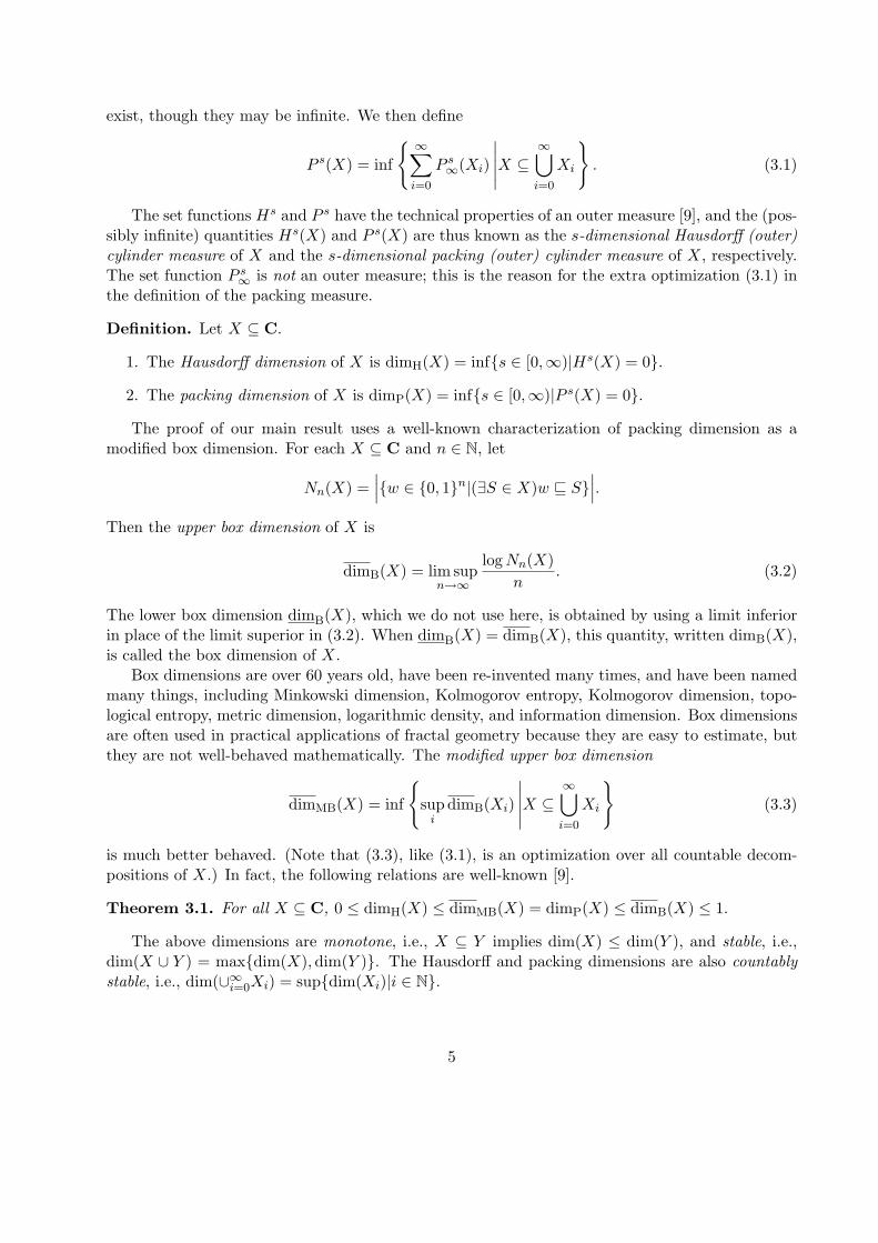
exist, though they may be infinite. We then define
P s(X) = inf
∞∑i=0
P s∞(Xi)
∣∣∣∣∣X ⊆∞⋃i=0
Xi
. (3.1)
The set functions Hs and P s have the technical properties of an outer measure [9], and the (pos-sibly infinite) quantities Hs(X) and P s(X) are thus known as the s-dimensional Hausdorff (outer)cylinder measure of X and the s-dimensional packing (outer) cylinder measure of X, respectively.The set function P s
∞ is not an outer measure; this is the reason for the extra optimization (3.1) inthe definition of the packing measure.
Definition. Let X ⊆ C.
1. The Hausdorff dimension of X is dimH(X) = infs ∈ [0,∞)|Hs(X) = 0.
2. The packing dimension of X is dimP(X) = infs ∈ [0,∞)|P s(X) = 0.
The proof of our main result uses a well-known characterization of packing dimension as amodified box dimension. For each X ⊆ C and n ∈ N, let
Nn(X) =∣∣∣w ∈ 0, 1n|(∃S ∈ X)w v S
∣∣∣.Then the upper box dimension of X is
dimB(X) = lim supn→∞
log Nn(X)n
. (3.2)
The lower box dimension dimB(X), which we do not use here, is obtained by using a limit inferiorin place of the limit superior in (3.2). When dimB(X) = dimB(X), this quantity, written dimB(X),is called the box dimension of X.
Box dimensions are over 60 years old, have been re-invented many times, and have been namedmany things, including Minkowski dimension, Kolmogorov entropy, Kolmogorov dimension, topo-logical entropy, metric dimension, logarithmic density, and information dimension. Box dimensionsare often used in practical applications of fractal geometry because they are easy to estimate, butthey are not well-behaved mathematically. The modified upper box dimension
dimMB(X) = inf
sup
idimB(Xi)
∣∣∣∣∣X ⊆∞⋃i=0
Xi
(3.3)
is much better behaved. (Note that (3.3), like (3.1), is an optimization over all countable decom-positions of X.) In fact, the following relations are well-known [9].
Theorem 3.1. For all X ⊆ C, 0 ≤ dimH(X) ≤ dimMB(X) = dimP(X) ≤ dimB(X) ≤ 1.
The above dimensions are monotone, i.e., X ⊆ Y implies dim(X) ≤ dim(Y ), and stable, i.e.,dim(X ∪ Y ) = maxdim(X),dim(Y ). The Hausdorff and packing dimensions are also countablystable, i.e., dim(∪∞i=0Xi) = supdim(Xi)|i ∈ N.
5

4 Gale Characterizations
In this section we review the gale characterization of Hausdorff dimension and prove our maintheorem, which is the dual gale characterization of packing dimension.
Definition. Let s ∈ [0,∞).
1. An s-supergale is a function d : 0, 1∗ −→ [0,∞) that satisfies the condition
d(w) ≥ 2−s[d(w0) + d(w1)] (4.1)
for all w ∈ 0, 1∗.
2. An s-gale is an s-supergale that satisfies (4.1) with equality for all w ∈ 0, 1∗.
3. A supermartingale is a 1-supergale.
4. A martingale is a 1-gale.
Intuitively, we regard a supergale d as a strategy for betting on the successive bits of a sequenceS ∈ C. More specifically d(w) is the amount of capital that d has after betting on the prefix wof S. If s = 1, then the right-hand side of (4.1) is the conditional expectation of d(wb) given thatw has occurred (when b is a uniformly distributed binary random variable). Thus a martingalemodels a gambler’s capital when the payoffs are fair. (The expected capital after the bet is theactual capital before the bet.) In the case of an s-gale, if s < 1, the payoffs are less than fair; ifs > 1, the payoffs are more than fair.
We use the following known generalization of the Kraft inequality.
Lemma 4.1. (Lutz [22]) Let s ∈ [0,∞). If d is an s-supergale and B ⊆ 0, 1∗ is a prefix set, thenfor all w ∈ 0, 1∗,
∑u∈B 2−s|u|d(wu) ≤ d(w).
We now define two criteria for the success of a gale or supergale.
Definition. Let d be an s-supergale, where s ∈ [0,∞).
1. We say that d succeeds on a sequence S ∈ C if
lim supn→∞
d(S[0..n− 1]) = ∞. (4.2)
The success set of d is S∞[d] = S ∈ C|d succeeds on S.
2. We say that d succeeds strongly on a sequence S ∈ C if
lim infn→∞
d(S[0..n− 1]) = ∞. (4.3)
The strong success set of d is S∞str[d] = S ∈ C|d succeeds strongly on S.
We have written conditions (4.2) and (4.3) in a fashion that emphasizes their duality. Condition(4.2) says simply that the set of values d(S[0..n− 1]) is unbounded, while condition (4.3) says thatd(S[0..n− 1]) →∞ as n →∞.
Notation. Let X ⊆ C.
6
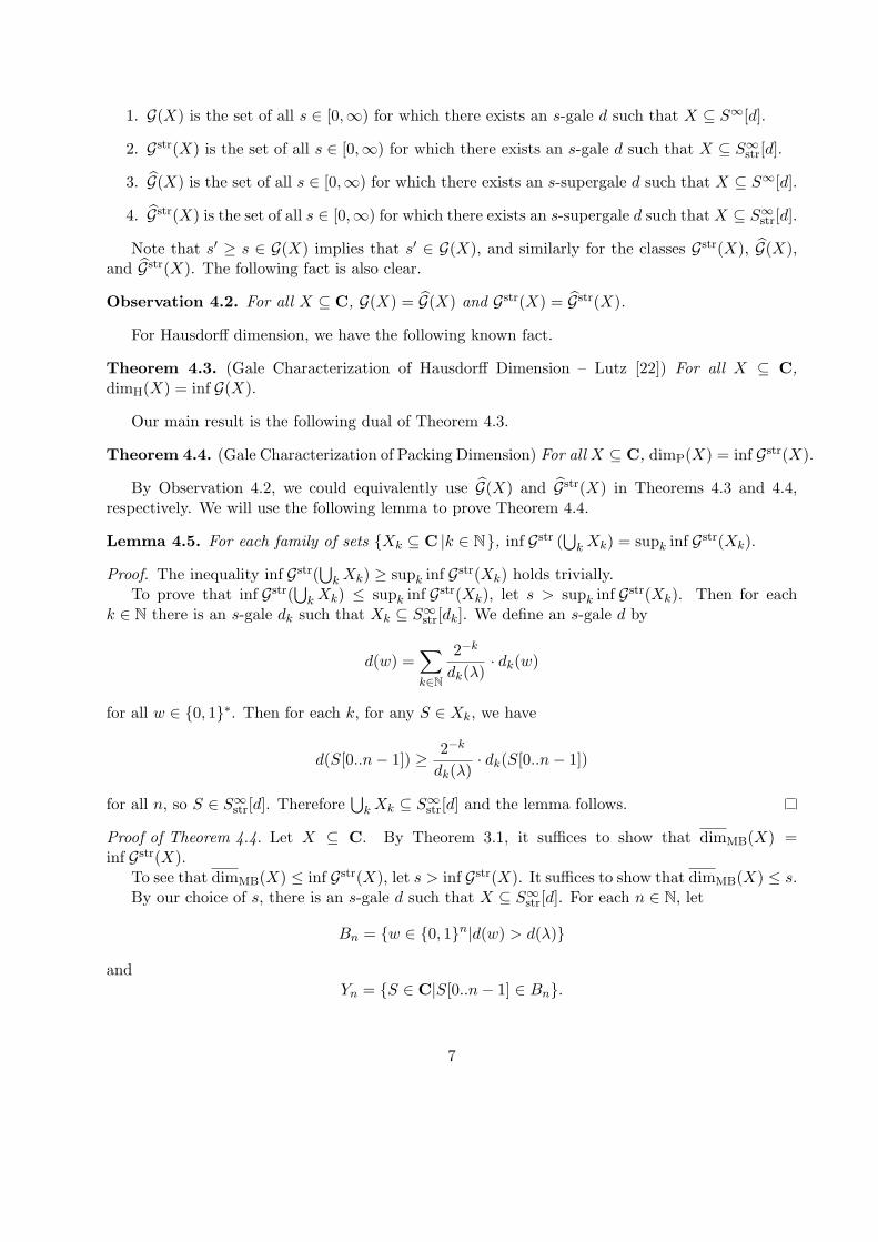
1. G(X) is the set of all s ∈ [0,∞) for which there exists an s-gale d such that X ⊆ S∞[d].
2. Gstr(X) is the set of all s ∈ [0,∞) for which there exists an s-gale d such that X ⊆ S∞str[d].
3. G(X) is the set of all s ∈ [0,∞) for which there exists an s-supergale d such that X ⊆ S∞[d].
4. Gstr(X) is the set of all s ∈ [0,∞) for which there exists an s-supergale d such that X ⊆ S∞str[d].
Note that s′ ≥ s ∈ G(X) implies that s′ ∈ G(X), and similarly for the classes Gstr(X), G(X),and Gstr(X). The following fact is also clear.
Observation 4.2. For all X ⊆ C, G(X) = G(X) and Gstr(X) = Gstr(X).
For Hausdorff dimension, we have the following known fact.
Theorem 4.3. (Gale Characterization of Hausdorff Dimension – Lutz [22]) For all X ⊆ C,dimH(X) = inf G(X).
Our main result is the following dual of Theorem 4.3.
Theorem 4.4. (Gale Characterization of Packing Dimension) For all X ⊆ C, dimP(X) = inf Gstr(X).
By Observation 4.2, we could equivalently use G(X) and Gstr(X) in Theorems 4.3 and 4.4,respectively. We will use the following lemma to prove Theorem 4.4.
Lemma 4.5. For each family of sets Xk ⊆ C |k ∈ N, inf Gstr (⋃
k Xk) = supk inf Gstr(Xk).
Proof. The inequality inf Gstr(⋃
k Xk) ≥ supk inf Gstr(Xk) holds trivially.To prove that inf Gstr(
⋃k Xk) ≤ supk inf Gstr(Xk), let s > supk inf Gstr(Xk). Then for each
k ∈ N there is an s-gale dk such that Xk ⊆ S∞str[dk]. We define an s-gale d by
d(w) =∑k∈N
2−k
dk(λ)· dk(w)
for all w ∈ 0, 1∗. Then for each k, for any S ∈ Xk, we have
d(S[0..n− 1]) ≥ 2−k
dk(λ)· dk(S[0..n− 1])
for all n, so S ∈ S∞str[d]. Therefore⋃
k Xk ⊆ S∞str[d] and the lemma follows.
Proof of Theorem 4.4. Let X ⊆ C. By Theorem 3.1, it suffices to show that dimMB(X) =inf Gstr(X).
To see that dimMB(X) ≤ inf Gstr(X), let s > inf Gstr(X). It suffices to show that dimMB(X) ≤ s.By our choice of s, there is an s-gale d such that X ⊆ S∞str[d]. For each n ∈ N, let
Bn = w ∈ 0, 1n|d(w) > d(λ)
andYn = S ∈ C|S[0..n− 1] ∈ Bn.
7
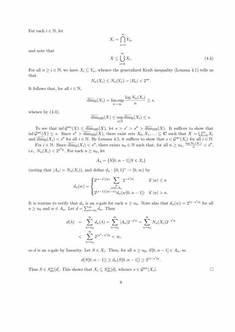
For each i ∈ N, let
Xi =∞⋂
n=i
Yn,
and note that
X ⊆∞⋃i=0
Xi. (4.4)
For all n ≥ i ∈ N, we have Xi ⊆ Yn, whence the generalized Kraft inequality (Lemma 4.1) tells usthat
Nn(Xi) ≤ Nn(Yn) = |Bn| < 2sn.
It follows that, for all i ∈ N,
dimB(Xi) = lim supn→∞
log Nn(Xi)n
≤ s,
whence by (4.4),dimMB(X) ≤ sup
i∈NdimB(Xi) ≤ s.
To see that inf Gstr(X) ≤ dimMB(X), let s > s′ > s′′ > dimMB(X). It suffices to show thatinf Gstr(X) ≤ s. Since s′′ > dimMB(X), there exist sets X0, X1, . . . ⊆ C such that X =
⋃∞i=0 Xi
and dimB(Xi) < s′′ for all i ∈ N. By Lemma 4.5, it suffices to show that s ∈ Gstr(Xi) for all i ∈ N.Fix i ∈ N. Since dimB(Xi) < s′′, there exists n0 ∈ N such that, for all n ≥ n0,
log Nn(Xi)n < s′′,
i.e., Nn(Xi) < 2s′′n. For each n ≥ n0, let
An = S[0..n− 1]|S ∈ Xi
(noting that |An| = Nn(Xi)), and define dn : 0, 1∗ → [0,∞) by
dn(w) =
2(s−s′)|w|
∑u
wu∈An
2−s′|u| if |w| ≤ n
2(s−1)(|w|−n)dn(w[0..n− 1]) if |w| > n.
It is routine to verify that dn is an s-gale for each n ≥ n0. Note also that dn(w) = 2(s−s′)n for alln ≥ n0 and w ∈ An. Let d =
∑∞n=n0
dn. Then
d(λ) =∞∑
n=n0
dn(λ) =∞∑
n=n0
|An|2−s′n =∞∑
n=n0
Nn(Xi)2−s′n
<
∞∑n=n0
2(s′′−s′)n < ∞,
so d is an s-gale by linearity. Let S ∈ Xi. Then, for all n ≥ n0, S[0..n− 1] ∈ An, so
d(S[0..n− 1]) ≥ dn(S[0..n− 1]) ≥ 2(s−s′)n.
Thus S ∈ S∞str[d]. This shows that Xi ⊆ S∞str[d], whence s ∈ Gstr(Xi).
8
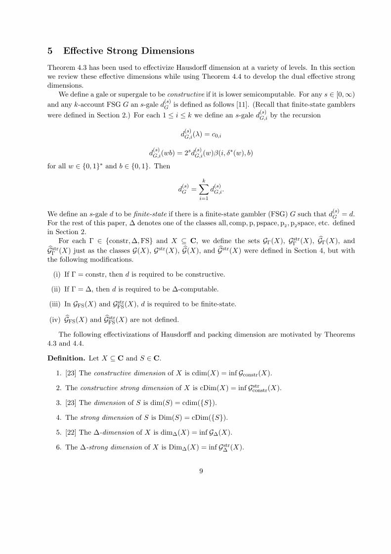
5 Effective Strong Dimensions
Theorem 4.3 has been used to effectivize Hausdorff dimension at a variety of levels. In this sectionwe review these effective dimensions while using Theorem 4.4 to develop the dual effective strongdimensions.
We define a gale or supergale to be constructive if it is lower semicomputable. For any s ∈ [0,∞)and any k-account FSG G an s-gale d
(s)G is defined as follows [11]. (Recall that finite-state gamblers
were defined in Section 2.) For each 1 ≤ i ≤ k we define an s-gale d(s)G,i by the recursion
d(s)G,i(λ) = c0,i
d(s)G,i(wb) = 2sd
(s)G,i(w)β(i, δ∗(w), b)
for all w ∈ 0, 1∗ and b ∈ 0, 1. Then
d(s)G =
k∑i=1
d(s)G,i.
We define an s-gale d to be finite-state if there is a finite-state gambler (FSG) G such that d(s)G = d.
For the rest of this paper, ∆ denotes one of the classes all, comp,p,pspace,p2 ,p2space, etc. definedin Section 2.
For each Γ ∈ constr,∆,FS and X ⊆ C, we define the sets GΓ(X), GstrΓ (X), GΓ(X), and
GstrΓ (X) just as the classes G(X), Gstr(X), G(X), and Gstr(X) were defined in Section 4, but with
the following modifications.
(i) If Γ = constr, then d is required to be constructive.
(ii) If Γ = ∆, then d is required to be ∆-computable.
(iii) In GFS(X) and GstrFS(X), d is required to be finite-state.
(iv) GFS(X) and GstrFS(X) are not defined.
The following effectivizations of Hausdorff and packing dimension are motivated by Theorems4.3 and 4.4.
Definition. Let X ⊆ C and S ∈ C.
1. [23] The constructive dimension of X is cdim(X) = inf Gconstr(X).
2. The constructive strong dimension of X is cDim(X) = inf Gstrconstr(X).
3. [23] The dimension of S is dim(S) = cdim(S).
4. The strong dimension of S is Dim(S) = cDim(S).
5. [22] The ∆-dimension of X is dim∆(X) = inf G∆(X).
6. The ∆-strong dimension of X is Dim∆(X) = inf Gstr∆ (X).
9
7. [22] The dimension of X in R(∆) is dim(X|R(∆)) = dim∆(X ∩R(∆)).
8. The strong dimension of X in R(∆) is Dim(X|R(∆)) = Dim∆(X ∩R(∆)).
9. [11] The finite-state dimension of X is dimFS(X) = inf GFS(X).
10. The finite-state strong dimension of X is DimFS(X) = inf GstrFS(X).
11. [11] The finite-state dimension of S is dimFS(S) = dimFS(S).
12. The finite-state strong dimension of S is DimFS(S) = DimFS(S).
In parts 1, 2, 5, and 6 of the above definition, we could equivalently use the “hatted” setsGconstr(X), Gstr
constr(X), G∆(X), and Gstr∆ (X) in place of their unhatted counterparts. In the case of
parts 5 and 6, this follows from Lemma 4.7 of [22]. In the case of parts 1 and 2, it follows from themain theorem in [15] (which answered an open question in [23], where Gconstr(X) was in fact usedin defining cdim(X)).
The polynomial-time dimensions dimp(X) and Dimp(X) are also called the feasible dimensionand the feasible strong dimension, respectively. The notation dimp(X) for the p-dimension is alltoo similar to the notation dimP(X) for the classical packing dimension, but confusion is unlikelybecause these dimensions typically arise in quite different contexts.
Note that the classical Hausdorff and packing dimensions can each now be written in threedifferent ways, i.e.,
dimH(X) = dimall(X) = dim(X|C)
anddimP(X) = Dimall(X) = Dim(X|C).
Observations 5.1. 1. Each of the dimensions that we have defined is monotone (e.g., X ⊆ Yimplies cdim(X) ≤ cdim(Y )).
2. Each of the effective strong dimensions is bounded below by the corresponding effective dimen-sion (e.g., cdim(X) ≤ cDim(X)).
3. Each of the dimensions that we have defined is nonincreasing as the effectivity constraint isrelaxed (e.g., dimH(X) ≤ cdim(X) ≤ dimpspace(X) ≤ dimFS(X)).
4. Each of the dimensions that we have defined is nonnegative and assigns C the dimension 1.
Lemma 5.2. The finite-state dimensions are stable, i.e., for all X, Y ⊆ C,
dimFS(X ∪ Y ) = maxdimFS(X),dimFS(Y )
andDimFS(X ∪ Y ) = maxDimFS(X),DimFS(Y ).
Proof. The stability of finite-state dimension was proved in [11]. The same arguments establishstability for finite-state strong dimension.
Definition. Let X, X0, X1, X2, . . . ⊆ C.
10
1. We say that X is a ∆-union of the ∆-dimensioned sets Xk|k ∈ N if X =⋃∞
k=0 Xk and foreach s > supk∈N dim∆(Xk) with 2s rational, there is a function d : N× 0, 1∗ → [0,∞) withthe following three properties.
(i) d is ∆-computable.
(ii) For each k ∈ N, if we write dk(w) = d(k, w), then the function dk is an s-gale.
(iii) For each k ∈ N, Xk ⊆ S∞[dk].
Analogously, X is a ∆-union of the ∆-strong dimensioned sets Xk|k ∈ N if there is a d withthe above properties that also satisfies
(iv) For each k ∈ N, Xk ⊆ S∞str[dk].
2. We say that X is a ∆-union of the sets Xk|k ∈ N dimensioned in R(∆) if X =⋃∞
k=0 Xk
and X ∩R(∆) is a ∆-union of the ∆-dimensioned sets Xk ∩R(∆)|k ∈ N.Analogously, X is a ∆-union of the sets Xk|k ∈ N strong dimensioned in R(∆) if X =⋃∞
k=0 Xk and X ∩R(∆) is an ∆-union of the ∆-strong dimensioned sets Xk ∩R(∆)|k ∈ N.
Lemma 5.3. The dimensions defined from ∆ are ∆-countably stable, i.e., if X is a ∆-union ofthe ∆-dimensioned sets X0, X1, X2, . . . , then
dim∆(X) = supk∈N
dim∆(Xk),
and if X is a ∆-union of the ∆-strong dimensioned sets X0, X1, X2, . . ., then
Dim∆(X) = supk∈N
Dim∆(Xk),
and similarly for dimension and strong dimension in R(∆).
Proof. The stability of dim∆ over ∆-unions was proved in [22]. The proof for strong dimension isanalogous.
Lemma 5.4. The constructive dimensions are absolutely stable, i.e., for all X ⊆ C,
cdim(X) = supS∈X
dim(S)
andcDim(X) = sup
S∈XDim(S).
Proof. The absolute stability of constructive dimension was proved in [23] using optimal construc-tive supergales. The same argument works for constructive strong dimension.
In the following two sections, we use Martin-Lof’s definition of randomness [24] as reformulatedin terms of martingales by Schnorr [32] as follows.
A probability measure on C is a function ν : 0, 1∗ → [0,∞) such that ν(λ) = 1 and ν(w) =ν(w0) + ν(w1) for all w ∈ 0, 1∗. (Intuitively, ν(w) is the probability that w v S when thesequence S is “chosen according to ν.”)
11
A bias is a real number β ∈ [0, 1]. Intuitively, if we toss a 0/1-valued coin with bias β, then βis the probability of the outcome 1. A bias sequence is a sequence ~β = (β0, β1, β2, . . .) of biases. If~β is a bias sequence, then the ~β-coin-toss probability measure is the probability µ
~β on C defined by
µ~β(w) =
|w|−1∏i=0
βi(w), (5.1)
where βi(w) = (2βi − 1)w[i] + (1− βi), i.e., βi(w) = if w[i] then βi else 1− βi. That is, µ~β is the
probability that S ∈ Cw when S ∈ C is chosen according to a random experiment in which foreach i, independently of all other j, the ith bit of S is decided by tossing a 0/1-valued coin whoseprobability of 1 is βi. In the case where the biases βi are all the same, i.e., ~β = (β, β, β, . . .) forsome β ∈ [0, 1], we write µβ for µ
~β, and (5.1) simplifies to
µβ(w) = (1− β)#(0,w)β#(1,w), (5.2)
where #(b, w) is the number of times the bit b appears in the string w. The uniform probabilitymeasure on C is the probability measure µ = µ
12 , for which (5.2) simplifies to
µ(w) = 2−|w|
for all w ∈ 0, 1∗.
Definition. Let ν be a probability measure on C.
1. A ν-martingale is a function d : 0, 1∗ → [0,∞) that satisfies the condition
d(w)ν(w) = d(w0)ν(w0) + d(w1)ν(w1)
for all w ∈ 0, 1∗.
2. A ν-martingale is constructive if it is lower semicomputable.
Note that a µ-martingale is a martingale. If ~β is a bias sequence, then we call a µ~β-martingale
simply a ~β-martingale.
Definition. Let ν be a probability measure on C, and let X ⊆ C.
1. X has constructive ν-measure 0, and we write νconstr(X) = 0, if there is a constructive ν-martingale d such that X ⊆ S∞[d].
2. X has constructive ν-measure 1, and we write νconstr(X) = 1, if νconstr(C−X) = 0.
Definition. If ν is a probability measure on C, then a sequence R ∈ C is ν-random, and we writeR ∈ RANDν , if the singleton set R does not have constructive ν-measure 0 (i.e., there is noconstructive ν-martingale that succeeds on R).
It is well-known (and easy to see) that νconstr(RANDν) = 1.
We write RAND~β for RANDµ~β
and RAND for RANDµ.We also use resource-bounded notions of randomness that have been investigated by Schnorr
[33], Lutz [20], Ambos-Spies, Terwijn, and Zheng [2], and others.
12
Definition. Let ν be a probability measure on C, and let t : N → N.
1. A sequence R ∈ C is ∆-ν-random, and we write R ∈ RANDν(∆), if there is no ∆-computableν-martingale that succeeds on R.
2. A sequence R ∈ C is t(n)-ν-random, and we write R ∈ RANDν(t(n)), if there is no O(t(n))-time-computable ν-martingale that succeeds on R.
We write RAND~β(t(n)) for RANDµ~β(t(n)).
6 Algorithmic Information
In this section we present a variety of results and observations in which constructive and computablestrong dimensions illuminate or clarify various aspects of algorithmic information theory. Includedis our second main theorem, which says that every sequence that is random with respect to acomputable sequence of biases βi ∈ [δ, 1/2] has the lower and upper average entropies of (β0, β1, . . .)as its dimension and strong dimension, respectively. We also present a result in which finite-statestrong dimension clarifies an issue in data compression.
Mayordomo [26] proved that for all S ∈ C,
dim(S) = lim infn→∞
K(S[0..n− 1])n
, (6.1)
where K(w) is the Kolmogorov complexity of w. (Note: Here and below, K(w) is the “self-delimiting”, or “prefix”, version of Kolmogorov complexity, as opposed to the “plain” complexityC(w) [19].) Subsequently, Lutz [23] used termgales to define the dimension dim(w) of each (finite!)string w ∈ 0, 1∗ and proved that
dim(S) = lim infn→∞
dim(S[0..n− 1]) (6.2)
for all S ∈ C andK(w) = |w|dim(w)±O(1) (6.3)
for all w ∈ 0, 1∗, thereby giving a second proof of (6.1). The following theorem is a dual of (6.2)that yields a dual of (6.1) as a corollary.
Theorem 6.1. For all S ∈ C,
Dim(S) = lim supn→∞
dim(S[0..n− 1]).
Proof. This proof is analogous to the one for the dual statement (6.2) given in [23].
Corollary 6.2. For all S ∈ C,
Dim(S) = lim supn→∞
K(S[0..n− 1])n
.
13

By Corollary 6.2, the “upper algorithmic dimension” defined by Tadaki [41] is precisely theconstructive strong dimension.
The rate at which a gambler can increase its capital when betting in a given situation is afundamental concern of classical and algorithmic information and computational learning theories.In the setting of constructive gamblers, the following quantities are of particular relevance.
Definition. Let d be a supermartingale, let S ∈ C, and let X ⊆ C.
1. The lower d-Lyapunov exponent of S is λd(S) = lim infn→∞log d(S[0..n−1])
n .
2. The upper d-Lyapunov exponent of S is Λd(S) = lim supn→∞log d(S[0..n−1])
n .
3. The lower Lyapunov exponent of S is λ(S) = supλd(S)|d is a constructive supermartingale.
4. The upper Lyapunov exponent of S is Λ(S) = supΛd(S)|d is a constructive supermartingale.
5. The lower Lyapunov exponent of X is λ(X) = infS∈X λ(S).
6. The upper Lyapunov exponent of X is Λ(X) = infS∈X Λ(S).
Lyapunov exponents such as these were investigated by Schnorr [33, 35], Ryabko [31], andStaiger [38, 39] (using slightly different notations) prior to the effectivization of Hausdorff dimension.The quantities λd(S) and Λd(S) are also called “exponents of increase” of d on S. It is implicit inStaiger’s paper [38] that
Λcomp(S) = 1− dimcomp(S)
for all S ∈ C, where Λcomp(S) is defined like Λ(S) above, but with d required to be a computablemartingale. Similar reasoning leads to the following characterizations of the Lyapunov exponents.
Theorem 6.3. Let S ∈ C and X ⊆ C. Then Λ(S) = 1 − dim(S), λ(S) = 1 − Dim(S), Λ(X) =1− cdim(X), and λ(X) = 1− cDim(X).
Proof. We show that Λ(S) = 1 − dim(S). A similar argument shows that λ(S) = 1 − Dim(S).By Lemma 5.4, Λ(X) = 1− cdim(X) and λ(X) = 1− cDim(X) follow from the statements aboutsequences.
Let t < s < Λ(S) with t computable, and let d be a constructive supermartingale for whichΛd(S) > s. Then for infinitely many n, d(S[0..n − 1]) > 2sn. Define a constructive (1 − t)-supergale d′ by d′(w) = 2−t|w|d(w) for all w ∈ 0, 1∗. Then for infinitely many n, we haved′(S[0..n− 1]) = 2−tnd(S[0..n− 1]) > 2(s−t)n, so S ∈ S∞[d]. Therefore dim(S) ≤ 1− t. This holdsfor all computable t < Λ(S), so dim(S) ≤ 1− Λ(S).
Let s > dim(S) be computable, and let d be a constructive s-gale with S ∈ S∞[d]. Define aconstructive martingale d′ by d′(w) = 2(1−s)|w|d(w) for all w ∈ 0, 1∗. For infinitely many n, wehave d(S[0..n− 1]) > 1, and for each of these n, d′(S[0..n− 1]) > 2(1−s)n. Therefore Λd′(S) ≥ 1− s,so Λ(S) ≥ 1− s. This holds for all s > dim(S), so Λ(S) ≥ 1− dim(S).
Constructive strong dimension can also be used to characterize entropy rates of the type inves-tigated by Staiger [37, 38] and Hitchcock [16].
Definition. Let A ⊆ 0, 1∗.
1. The entropy rate of A ⊆ 0, 1∗ is HA = lim supn→∞log |A=n|
n .
14
2. We define the sets of sequences
Ai.o. = S ∈ C|(∃∞n)S[0..n− 1] ∈ A
andAa.e. = S ∈ C|(∀∞n)S[0..n− 1] ∈ A.
Definition. Let X ⊆ C. The constructive entropy rate of X is
HCE(X) = infHA|X ⊆ Ai.o. and A ∈ CE
and the constructive strong entropy rate of X is
HstrCE(X) = infHA|X ⊆ Aa.e. and A ∈ CE.
Hitchcock [16] proved thatHCE(X) = cdim(X) (6.4)
for all X ⊆ C. We have the following dual of (6.4).
Theorem 6.4. For any X ⊆ C, HstrCE(X) = cDim(X).
Proof. This proof is analogous to the proof of (6.4) given in [16].
In the classical case, Tricot [42] has defined a set to be regular if its Hausdorff and packingdimensions coincide, and defined its irregularity to be the difference between these two fractaldimensions. Analogously, we define the c-irregularity (i.e., constructive irregularity) of a sequenceS ∈ C to be Dim(S) − dim(S), and we define the c-irregularity of a set X ⊆ C to be cDim(X) −cdim(X). We define a sequence or set to be c-regular (i.e., constructively regular) if its c-irregularityis 0.
As the following result shows, the c-irregularity of a sequence may be any real number in [0, 1].
Theorem 6.5. For any two real numbers 0 ≤ α ≤ β ≤ 1, there is a sequence S ∈ C such thatdim(S) = α and Dim(S) = β.
Proof. Let R ∈ RAND be a random sequence. It is well-known that
K(R[0..n− 1]) ≥ n−O(1). (6.5)
Write R = r1r2r3 . . . where |rn| = 2n− 1 for all n. Note that |r1 · · · rn| = n2.For each n, define
γn =
1−α
α if log∗ n is odd1−β
β if log∗ n is even,
and letkn = d|rn|γne .
We now define S ∈ C asS = r10k1r20k2 · · · rn0kn · · · .
15
Note that for all n,
|rn0kn | = d|rn|(1 + γn)e
=
⌈1α |rn|
⌉if log∗ n is odd⌈
1β |rn|
⌉if log∗ n is even.
Let w v S. Then for some n,
w = r10k1 · · · rn−10kn−1r′n0j
where r′n v rn and 0 ≤ j ≤ kn. We have
K(w) ≤ K(r1 · · · rn−1r′n) + K(k1) + · · ·+ K(kn−1) + K(j) + O(1)
≤ |r1 · · · rn−1r′n|+ O(n log n)
≤ (n− 1)2 + O(n log n).
(6.6)
Also,
K(r1 · · · rn−1r′n) ≤ K(w) + K(k1) + · · ·+ K(kn−1) + K(j) + O(1)
≤ K(w) + O(n log n),
so by (6.5),K(w) ≥ K(r1 · · · rn−1r
′n)−O(n log n)
≥ |r1 · · · rn−1r′n| −O(n log n)
≥ (n− 1)2 −O(n log n).
(6.7)
We bound the length of w in terms of n as
|w| ≥ |r1|(1 + γ1) + · · ·+ |rn−1|(1 + γn−1) + |r′n|
≥ |r1 · · · rn−1|β
=1β
(n− 1)2
(6.8)
and|w| ≤ |r1|(1 + γ1) + · · ·+ |rn−1|(1 + γn−1) + |rn|(1 + γn) + n
≤ |r1 · · · rn−1rn|α
+ n
≤ 1α
(n + 1)2.
(6.9)
From (6.6) and (6.8), we have
lim supm→∞
K(S[0..m− 1])m
≤ lim supn→∞
(n− 1)2 + O(n log n)1β (n− 1)2
= β, (6.10)
and (6.7) and (6.9) yield
lim infm→∞
K(S[0..m− 1])m
≥ lim infn→∞
(n− 1)2 −O(n log n)1α(n + 1)2
= α. (6.11)
16
For each n, letwn = r10k1 · · · rn0kn .
Recall the sequence of towers defined by tj by t0 = 1 and tj+1 = 2tj . If j is even, then for alltj−1 < i ≤ tj , γi = 1−β
β . Then
|wtj | ≤ tj +tj∑
i=1
|ri|(1 + γi)
= tj +tj−1∑i=1
|ri|(1 + γi) +1β
tj∑i=tj−1+1
|ri|
≤ tj +1α
t2j−1 +1β
(t2j − t2j−1)
≤ 1β
t2j + tj + O((log tj)2).
(6.12)
Similarly, if j is odd, we have
|wtj | ≥tj∑
i=1
|ri|(1 + γi)
=tj−1∑i=1
|ri|(1 + γi) +1α
tj∑i=tj−1+1
|ri|
≥ 1β
tj−12 +
1α
(t2j − t2j−1)
≥ 1α
t2j −O((log tj)2).
(6.13)
Combining (6.7) and (6.12), we have
lim supm→∞
K(S[0..m− 1])m
≥ lim supn→∞
K(wt2n)|wt2n |
≥ β. (6.14)
Putting (6.6) together with (6.13) yields
lim infm→∞
K(S[0..m− 1])m
≤ lim infn→∞
K(wt2n+1)|wt2n+1 |
≤ α. (6.15)
By (6.1), (6.11), and (6.15), we have dim(S) = α. By Corollary 6.2, (6.10), and (6.14), we haveDim(S) = β.
We now come to the main theorem of this section. The following notation simplifies its statementand proof.
Notation. Given a bias sequence ~β = (β0, β1, . . .), n ∈ N, and S ∈ C, let
Hn(~β) =1n
n−1∑i=0
H(βi),
H−(~β) = lim infn→∞
Hn(~β),
H+(~β) = lim supn→∞
Hn(~β).
17
We call H−(~β) and H+(~β) the lower and upper average entropies, respectively, of ~β.
Theorem 6.6. If δ ∈ (0, 12 ] and ~β is a computable bias sequence with each βi ∈ [δ, 1
2 ], then for
every sequence R ∈ RAND~β,
dim(R) = H−(~β) and Dim(R) = H+(~β).
Theorem 6.6 says that every sequence that is random with respect to a suitable bias sequence ~βhas the lower and upper average entropies of ~β as its dimension and strong dimension, respectively.Since there exist ~β-random sequences in ∆0
2 when ~β is computable, this gives a powerful andflexible method for constructing ∆0
2 sequences with given (∆02-computable) dimensions and strong
dimensions.Note that Theorem 6.6 also gives an alternative, though less constructive, proof of Theorem
6.5.We now develop a sequence of results that are used in our proof of Theorem 6.6.
Lemma 6.7. Assume that δ > 0, ε > 0, and that, for each β ∈ [δ, 1− δ], ηβ is a bounded randomvariable with expectation Eηβ ≤ −ε and Eetηβ is, uniformly in t, a continuous function of β. Thenthere exists θ > 0 such that, for all β ∈ [δ, 1− δ] and t ∈ (0, θ],
Eetηβ < 1− tε
2.
Proof. Assume the hypothesis. Then the Dominated Convergence Theorem [3] tells us that, for allβ ∈ [δ, 1− δ],
limt→0+
Eetηβ − 1t
= limt→0+
Eetηβ − 1
t
= E(
limt→0+
etηβ − 1t
)= E
(ηβ lim
t→0+
etηβ − 1tηβ
)= Eηβ
≤ −ε.
Hence, for each β ∈ [δ, 1− δ], there exists tβ > 0 such that, for all t ∈ (0, tβ],
Eetηβ − 1t
< −3ε
4.
It follows by our continuity hypothesis that, for each β ∈ [δ, 1− δ], there is an open neighborhoodNβ of β such that, for all t ∈ (0, tβ] and γ ∈ Nβ ∩ [δ, 1− δ],
Eetηγ − 1t
< − ε
2.
The family G = Nβ | β ∈ [δ, 1−δ] is an open cover of the compact set [δ, 1−δ], so there is a finiteset B ⊆ [δ, 1− δ] such that the subcollection G′ = Nβ | β ∈ B is also a cover of [δ, 1− δ]. Let
θ = mintβ | β ∈ B.
18
Then θ > 0 and, for all β ∈ [δ, 1− δ] and t ∈ (0, θ],
Eetηβ − 1t
< − ε
2,
whenceEetηβ < 1− tε
2.
Corollary 6.8. For each δ > 0 and ε > 0, there exists θ > 0 such that, for all β ∈ [δ, 1− δ], if wechoose a ∈ 0, 1 with Prob[a = 1] = β, and if
η = ξ −H(β)− ε
orη = H(β)− ξ − ε,
whereξ = (1− a) log
11− β
+ a log1β
,
thenEeθη < 1− θε
2.
Proof. The random variables
η1,β = ξ −H(β)− ε,
η2,β = H(β)− ξ − ε
satisfy the hypothesis of Lemma 6.7 with Eη1,β = Eη2,β = −ε, so we can choose θ1 > 0 for η1,β andθ2 > 0 for η2,β as in that lemma. Letting θ = minθ1, θ2 establishes the corollary.
Notation. Given a bias sequence ~β = (β0, β1, . . .), n ∈ N, and S ∈ C, let
Ln(~β)(S) = log1
µ~β(S[0..n− 1])=
n−1∑i=0
ξi(S),
whereξi(S) = (1− S[i]) log
11− βi
+ S[i] log1βi
for 0 ≤ i < n.
Note that Ln(~β), ξ0, . . . , ξn−1 are random variables with
ELn(~β) =n−1∑i=0
Eξi =n−1∑i=0
H(βi) = nHn(~β).
The following large deviation theorem tells us that Ln(~β) is very unlikely to deviate significantlyfrom this expected value.
19
Theorem 6.9. For each δ > 0 and ε > 0, there exists α ∈ (0, 1) such that, for all bias sequences~β = (β0, β1, . . .) with each βi ∈ [δ, 1− δ] and all n ∈ Z+, if Ln(~β) and Hn(~β) are defined as above,then
P[|Ln(~β)− nHn(~β)| ≥ εn
]< 2αn,
where the probability is computed according to µ~β.
Proof. Let δ > 0 and ε > 0, and choose θ > 0 as in Corollary 6.8. Let α = 1 − θε2 , noting that
α ∈ (0, 1). Let ~β be as given, and let n ∈ Z+. Let L = Ln(~β), H = Hn(~β), and ξ0, ξ1, . . . be asabove. The proof is in two parts.
1. For each i ∈ N, let ηi = ξi−H(βi)−ε. Then Markov’s inequality, independence, and Corollary6.8 tell us that
P[L− nH ≥ εn] = P [eθ(L−nH) ≥ eθεn]≤ e−θεnEeθ(L−nH)
= Eeθ(L−nH)−εθn
= EeθPn−1
i=0 ηi
= En−1∏i=0
eθηi
=n−1∏i=0
Eeθηi
< αn.
2. Arguing as in part 1 with ηi = H(βi)− ξi − ε shows that P[nH − L ≥ εn] < αn.
By parts 1 and 2 of this proof, we now have
P[|L− nH| ≥ εn] < 2αn.
Some of our arguments are simplified by the following constructive version of a classical theoremof Kakutani [17]. Say that two bias sequences ~β and ~β′ are square-summably equivalent, and write~β ≈2 ~β′, if
∞∑i=0
(βi − β′i)2 < ∞.
Theorem 6.10. (van Lambalgen [43, 44], Vovk [46]) Let δ > 0, and let ~β and ~β′ be computablebias sequences with βi, β
′i ∈ [δ, 1− δ] for all i ∈ N.
1. If ~β ≈2 ~β′, then RAND~β = RAND~β′.
2. If ~β 6≈2 ~β′, then RAND~β ⋂RAND~β′
= ∅.
Corollary 6.11. If δ > 0 and ~β is a computable bias sequence with each βi ∈ [δ, 1− δ], then thereis an exactly computable bias sequence ~β′ with each β′i ∈ [ δ
2 , βi] satisfying RAND~β′= RAND~β.
20
Proof. Assume the hypothesis. Then there is a computable function g : N × N → Q such that|g(i, r)− βi| ≤ 2−r for all i, r ∈ N. Let m = 2 +
⌈log 1
δ
⌉, and let
β′i = g(i,m + i)− 2−(m+i)
for all i ∈ N. It is easily verified that ~β′ is exactly computable, each β′i ∈ [ δ2 , βi], and ~β′ ≈2 ~β,
whence Theorem 6.10 tells us that RAND~β′= RAND~β.
Lemma 6.12. If δ > 0 and ~β is a computable bias sequence with each βi ∈ [δ, 1 − δ], then everysequence R ∈ RAND~β satisfies
Ln(~β)(R) = nHn(~β) + o(n)
as n →∞.
Proof. Assume the hypothesis. By Corollary 6.11, we can assume that ~β is exactly computable.Let ε > 0. For each n ∈ N, define the set
Yn =
S ∈ C∣∣∣ |Ln(~β)(S)− nHn(~β)| ≥ εn
,
and letXε = S ∈ C | (∃∞n)S ∈ Yn.
It suffices to show that µ~βcomp(Xε) = 0.
For each n ∈ N and w ∈ 0, 1∗, let
dn(w) =
µ
~β(Yn|Cw) if |w| ≤ n
dn(w[0..n− 1]) if |w| > n.
It is easily verified that each dn is a ~β-martingale and that the function (n, w) 7→ dn(w) is com-putable. It is clear that Yn ⊆ S1[dn] for all n ∈ N, where S1[dn] =
⋃dn(w)≥1
Cw. Finally, by Theorem
6.9, the series∞∑
n=0dn(λ) is computably convergent, so the computable first Borel-Cantelli Lemma
[20] (extended to ~β as indicated in [4]) tells us that µ~βcomp(Xε) = 0.
Lemma 6.13. If δ > 0 and ~β is a computable bias sequence with each βi ∈ [δ, 12 ], then cdim(RAND~β) ≤
H−(~β) and cDim(RAND~β) ≤ H+(~β).
Proof. Assume the hypothesis. By Corollary 6.11, we can assume that ~β is exactly computable.Let s ∈ [0,∞) be computable.
Define d : 0, 1∗ → [0,∞) byd(w) = 2s|w|µ
~β(w)
for all w ∈ 0, 1∗. Then d is a constructive (in fact, computable) s-gale. For each R ∈ C andn ∈ N, if we write zn = R[0..n− 1], then
log d(zn) = sn + log µ~β(zn)
21
for all n. In particular, if R ∈ RAND~β, if follows by Lemma 6.12 that
log d(zn) = n[s−Hn(~β)] + o(n) (6.16)
as n →∞. We now verify the two parts of the lemma. For both parts, we let
Iε = n ∈ N | Hn(~β) < s− ε.
To see that cdim(RAND~β) ≤ H−(~β), let s > H−(~β), and let ε = s−H−(~β)2 . Then the set Iε is
infinite, so (6.16) tells us that RAND~β ⊆ S∞[d], whence cdim(RAND~β) ≤ s.
To see that cDim(RAND~β) ≤ H+(~β), let s > H+(~β), and let ε = s−H+(~β)2 . Then the set Iε is
cofinite, so (6.16) tells us that RAND~β ⊆ S∞str[d], whence cDim(RAND~β) ≤ s.
Lemma 6.14. Assume that δ > 0, ~β is a computable bias sequence with each βi ∈ [δ, 1 − δ],s ∈ [0,∞) is computable, and d is a constructive s-gale.
1. If s < H−(~β), then S∞[d]⋂
RAND~β = ∅.
2. If s < H+(~β), then S∞str[d]⋂
RAND~β = ∅.
Proof. Assume the hypothesis. Define d′ : 0, 1∗ → [0,∞) by
d′(w) =d(w)
2s|w|µ~β(w)
for all w ∈ 0, 1∗. Then d′ is a ~β-martingale, and d′ is clearly constructive.Let R ∈ RAND~β. Then d′ does not succeed on R, so there is a constant c > 0 such that, for all
n ∈ N, if we write zn = R[0..n− 1], then d′(zn) ≤ 2c, whence
log d(zn) ≤ c + sn + log µ~β(zn).
It follows by Lemma 6.12 that
log d(zn) ≤ c + n[s−Hn(~β)] + o(n)
as n →∞. Hence, for any ε > 0, if we let
Iε = n ∈ Z+ | s < Hn(~β)− ε,
then log d(zn) < c for all sufficiently large n ∈ Iε. We now verify the two parts of the lemma.
1. If s < H−(~β), let ε = H−(~β)−s2 . Then Iε is cofinite, so log d(zn) < c for all sufficiently large
n ∈ Z+, so R 6∈ S∞[d].
2. If s < H+(~β), let ε = H+(~β)−s2 . Then Iε is infinite, so log d(zn) < c for infinitely many n ∈ Z+,
so R 6∈ S∞str[d].
22
We now have all we need to prove the main theorem of this section.
Proof of Theorem 6.6. Assume the hypothesis, and let R ∈ RAND~β. By Lemma 6.13, dim(R) ≤H−(~β) and Dim(R) ≤ H+(~β). To see that dim(R) ≥ H−(~β) and Dim(R) ≥ H+(~β), let s, t ∈ [0,∞)be computable with s < H−(~β) and t < H+(~β), let d− be a constructive s-gale, and let d+ bea constructive t-gale. It suffices to show that R 6∈ S∞[d−] and R 6∈ S∞str[d
+]. But these followimmediately from Lemma 6.14 and the ~β-randomness of R.
Corollary 6.15. If ~β is a computable sequence of coin-toss biases such that H(~β) = limn→∞
Hn(~β) ∈
(0, 1), then every sequence R ∈ C that is random with respect to ~β is c-regular, with dim(R) =Dim(R) = H(~β).
Note that Corollary 6.15 strengthens Theorem 7.6 of [23] because the convergence of Hn(~β) isa weaker hypothesis than the convergence of ~β.
Generalizing the construction of Chaitin’s random real number Ω [6], Mayordomo [26] and,independently, Tadaki [41] defined for each s ∈ (0, 1] and each infinite, computably enumerable setA ⊆ 0, 1∗, the real number
θsA =
∑ 2−
|π|s
∣∣∣ π ∈ 0, 1∗ and U(π) ∈ A
,
where U is a universal self-delimiting Turing machine. Given (6.1) and Corollary 6.2 above, thefollowing fact is implicit in Tadaki’s paper.
Theorem 6.16. (Tadaki [41]) For each s ∈ (0, 1] and each infinite, computably enumerable setA ⊆ 0, 1∗, the (binary expansion of the) real number θs
A is c-regular with dim(θsA) = Dim(θs
A) = s.
We define a set X ⊆ C to be self-similar if it has the form
X = A∞ = S ∈ C | S = w0w1w2 . . . for some w0, w1, w2, . . . ∈ A
where A ⊆ 0, 1∗ is a finite prefix set. Self-similar sets are examples of c-regular sets.
Theorem 6.17. Let X = A∞ be self-similar where A is a finite prefix set. Then X is c-regular,with cdim(X) = cDim(X) = infs|
∑w∈A 2−s|w| ≤ 1.
Proof. We say that a string w is composite if there are strings w1, . . . , wk ∈ A such that w =w1 · · ·wk. Let s be computable such that
∑w∈A 2−s|w| ≤ 1. For any computable ε > 0 we define
a constructive (s + ε)-supergale d as follows. Let w ∈ 0, 1∗, and let v be the maximal compositeproper prefix of w. Then
d(w) =∑
u∈A:wvvu
2ε|w|2−s(|vu|−|w|).
For all composite strings w, we have d(w) = 2ε|w|. It follows that A∞ ⊆ S∞str[d], and thereforecDim(A∞) ≤ s + ε.
Let s such that∑
w∈A 2−s|w| > 1 and let d be an s-gale. To show that cdim(A∞) > s, it sufficesto construct a sequence S ∈ A∞ − S∞[d]. Initially, we let w0 = λ. Assume that wn has beendefined, and let u ∈ A such that d(wnu) ≤ d(wn). We know that such a u exists because of ourchoice of s. Then we let wn+1 = wnu. Our sequence S is the unique one that has wn v S for alln.
23
Dai, Lathrop, Lutz, and Mayordomo [7] investigated the finite-state compression ratio ρFS(S),defined for each sequence S ∈ C to be the infimum, taken over all information-lossless finite-statecompressors C (a model defined in Shannon’s 1948 paper [36]) of the (lower) compression ratio
ρC(S) = lim infn→∞
|C(S[0..n− 1])|n
.
They proved thatρFS(S) = dimFS(S) (6.17)
for all S ∈ C. However, it has been pointed out that the compression ratio ρFS(S) differs from theone investigated by Ziv [47]. Ziv was instead concerned with the ratio RFS(S) defined by
RFS(S) = infk∈N
lim supn→∞
infC∈Ck
|C(S[0..n− 1])|n
,
where Ck is the set of all k-state information-lossless finite-state compressors. The following result,together with (6.17), clarifies the relationship between ρFS(S) and RFS(S).
Theorem 6.18. For all S ∈ C, RFS(S) = DimFS(S).
The proof of Theorem 6.18 is based on the following lemma.
Lemma 6.19. Let C be the set of all finite-state compressors. For all S ∈ C,
RFS(S) = infC∈C
lim supn→∞
|C(S[0..n− 1])|n
.
Proof. For each k ∈ N let C′k be the set of all k-state information-lossless finite-state compressorswhose output length per input bit is bounded by k. Notice that C′k is a subset of Ck and that C′k isfinite. Ziv and Lempel implicitely prove in [48] that the following equality holds
RFS(S) = infk∈N
lim supn→∞
infC∈C′k
|C(S[0..n− 1])|n
.
LetR′
FS(S) = infC∈C
lim supn→∞
|C(S[0..n− 1])|n
.
The inequality RFS(S) ≤ R′FS(S) is trivial. We use several results from [7] to obtain for each k ∈ N
and ε > 0 a finite-state compressor Ck,ε that is nearly optimal for all compressors in C′k. FromLemma 7.7 in [7] we obtain a finite-state gambler for each C ∈ C′k. By Lemma 3.7 in [7], we cancombine these gamblers into a single finite-state gambler. Theorem 4.5 and Lemma 3.11 in [7]convert this single gambler into a 1-account nonvanishing finite-state gambler and finally Lemma7.10 converts this to the finite-state compressor Ck,ε. Combining the five cited constructions in [7]we obtain that there is a constant ck,ε such that for all w ∈ 0, 1∗ and C ∈ C′k,
|Ck,ε(w)| ≤ |C(w)|+ ε|w|+ ck,ε.
Then for all k ∈ N and ε > 0,
R′FS(S) ≤ lim sup
n→∞
|Ck,ε(S[0..n− 1])|n
≤ lim supn→∞
infC∈C′k
|C(S[0..n− 1])|n
+ ε,
so R′FS(S) ≤ RFS(S).
24
Proof of Theorem 6.18. The equality
DimFS(S) = infC∈C
lim supn→∞
|C(S[0..n− 1])|n
has a proof analogous to that of (6.17) given in [7]. Together with Lemma 6.19, this implies thatRFS(S) = DimFS(S).
Thus, mathematically, the compression ratios ρFS(S) and RFS(S) are both natural: they arethe finite-state effectivizations of the Hausdorff and packing dimensions, respectively.
7 Computational Complexity
In this section we prove our third main theorem, which says that the dimensions and strong dimen-sions of polynomial-time many-one degrees in exponential time are essentially unrestricted. Ourproof of this result uses Theorem 6.9 and convenient characterizations of p-dimension and strongp-dimension in terms of feasible unpredictability.
Definition. A predictor is a function π : 0, 1∗ × 0, 1 → [0, 1] such that for all w ∈ 0, 1∗,π(w, 0) + π(w, 1) = 1.
We interpret π(w, b) as the predictor’s estimate of the probability that the bit b will occur nextgiven that w has occurred. We write Π(p) for the class of all feasible predictors.
Definition. Let w ∈ 0, 1∗, S ∈ C, and X ⊆ C.
1. The cumulative log-loss of π on w is
Llog(π,w) =|w|−1∑i=0
log1
π(w[0..i− 1], w[i]).
2. The log-loss rate of π on S is
Llog(π, S) = lim infn→∞
Llog(π, S[0..n− 1])n
.
3. The strong log-loss rate of π on S is
Llogstr (π, S) = lim sup
n→∞
Llog(π, S[0..n− 1])n
.
4. The (worst-case) log-loss of π on X is
Llog(π,X) = supS∈X
Llog(π, S).
5. The (worst-case) strong log-loss of π on X is
Llogstr (π,X) = sup
S∈XLlog
str (π, S).
25
6. The feasible log-loss unpredictability of X is
unpredlogp (X) = inf
π∈Π(p)Llog(π,X).
7. The feasible strong log-loss unpredictability of X is
Unpredlogp (X) = inf
π∈Π(p)Llog
str (π,X).
Hitchcock [14] showed that feasible dimension exactly characterizes feasible log-loss unpre-dictability, that is,
unpredlogp (X) = dimp(X) (7.1)
for all X ⊆ C. The same argument proves the following dual result for strong dimension.
Theorem 7.1. For all X ⊆ C, Unpredlogp (X) = Dimp(X).
The following theorem is the main result of this section. Recall that the polynomial-time many-one degree of a language A ⊆ 0, 1∗ is
degPm(A) = Pm(A) ∩ P−1
m (A),
where the lower span Pm(A) and the upper span P−1m (A) are defined by
Pm(A) = B | B ≤Pm A, P−1
m (A) = B | A ≤Pm B.
Theorem 7.2. For every pair of ∆02-computable real numbers x, y with 0 < x ≤ y ≤ 1, there exists
A ∈ E such thatdimp(degP
m(A)) = dim(degPm(A)|E) = x
andDimp(degP
m(A)) = Dim(degPm(A)|E) = y.
Most of this section is devoted to proving Theorem 7.2. Our proof is motivated by analogous,but simpler, arguments by Ambos-Spies, Merkle, Reimann and Stephan [1]. Like most dimensioncalculations, our proof consists of separate lower and upper bound arguments. The results fromhere through Lemma 7.7 are used for the lower bound. Lemma 7.8 uses Theorem 7.1 to establishthe upper bound. The proof of Theorem 7.2 follows Lemma 7.8.
The first part of the following theorem is due to Ambos-Spies, Merkle, Reimann and Stephan[1]. The second part is an exact dual of the first part.
Theorem 7.3. Let A ∈ E.
1. dimp(degPm(A)) = dimp(Pm(A)) and dim(degP
m(A)|E) = dim(Pm(A)|E).
2. Dimp(degPm(A)) = Dimp(Pm(A)) and Dim(degP
m(A)|E) = Dim(Pm(A)|E).
The following lemma is a time-bounded version of Lemma 6.14.
Lemma 7.4. Assume that k, l ∈ Z+, δ > 0, ~β is an exactly nl-time-computable bias sequence witheach βi ∈ Q ∩ [δ, 1− δ], s ∈ Q ∩ [0,∞), and d is an nk-time-computable s-gale.
26
1. If s < H−(~β), then S∞[d]⋂
RAND~β(nk+2l+1) = ∅.
2. If s < H+(~β), then S∞str[d]⋂
RAND~β(nk+2l+1) = ∅.
Proof. We proceed exactly as in the proof of Lemma 6.14, noting that our present hypothesisimplies that the ~β-martingale d′ is O(nk+2l+1)-time-computable.
Our proof of Theorem 7.2 also uses the martingale dilation technique, which was introducedby Ambos-Spies, Terwijn, and Zheng [2] and extended by Breutzmann and Lutz [4]. Recall thestandard enumeration s0, s1, s2, . . . of 0, 1∗, defined in Section 2.
Definition. The restriction of a string w ∈ 0, 1∗ to a language A ⊆ 0, 1∗ is the string w Adefined by the following recursion.
1. λ A = λ.
2. For w ∈ 0, 1∗ and b ∈ 0, 1,
(wb) A =
(w A)b if s|w| ∈ A,
w A if s|w| 6∈ A.
(That is, w A is the concatenation of the successive bits w[i] for which si ∈ A.)
Definition. A function f : 0, 1∗ −→ 0, 1∗ is strictly increasing if, for all x, y ∈ 0, 1∗,
x < y =⇒ f(x) < f(y),
where < is the standard ordering of 0, 1∗.
Notation. If f : 0, 1∗ −→ 0, 1∗, then for each n ∈ N, let nf be the unique integer such thatf(sn) = snf
.
Definition. If f : 0, 1∗ −→ 0, 1∗ is strictly increasing and ~β is a bias sequence, then thef -dilation of ~β is the bias sequence ~βf given by βf
n = βnffor all n ∈ N.
Observation 7.5. If f : 0, 1∗ −→ 0, 1∗ is strictly increasing and A ⊆ 0, 1∗, then for alln ∈ N,
χf−1(A)[0..n− 1] = χA[0..nf − 1] range(f).
Definition. If f : 0, 1∗ −→ 0, 1∗ is strictly increasing and d is a martingale, then the f -dilationof d is the function f d : 0, 1∗ −→ [0,∞),
f d(w) = d(w range(f)).
Intuitively, the f -dilation of d is a strategy for betting on a language A, assuming that d itselfis a good betting strategy for betting on the language f−1(A). Given an opportunity to bet onthe membership of a string y = f(x) in A, f d bets exactly as d would bet on the membership ornonmembership of x in f−1(A).
The following result is a special case of Theorem 6.3 in [4].
27
Theorem 7.6. (Martingale Dilation Theorem - Breutzmann and Lutz [4]) Assume that ~β is a biassequence with each βi ∈ (0, 1), f : 0, 1∗ −→ 0, 1∗ is strictly increasing, and d is a ~βf -martingale.Then fˆd is a ~β-martingale and, for every language A ⊆ 0, 1∗, if d succeeds on f−1(A), then fˆdsucceeds on A.
Notation. For each k ∈ Z+, define gk : 0, 1∗ −→ 0, 1∗ by gk(x) = 0k|x|1x. Note that each gk
is strictly increasing and computable in polynomial time.
Lemma 7.7. Assume that ~β is a bias sequence with each βi ∈ (0, 1), and R ∈ RAND~β(n2). Then,for each k ≥ 2, g−1
k (R) ∈ RAND~α(nk), where ~α = ~βgk .
Proof. Let ~β, k, and ~α be as given, and assume that g−1k (R) 6∈ RAND~α(nk). Then there is an
nk-time-computable ~α-martingale d that succeeds on g−1k (R). It follows by Theorem 7.6 that gk d
is a ~β-martingale that succeeds on R. The time required to compute gk d(w) is O(|w|2 + |w′|k)steps, where w′ = w range(gk). (This allows O(|w|2) steps to compute w′ and then O(|w′|k) stepsto compute d(w′).) Now |w′| is bounded above by the number of strings x such that k|x|+ |x|+1 ≤|s|w|| = blog(1 + |w|)c. Therefore |w′| ≤ 21+log(1+|w|)/k, which implies |w′|k = O(|w|). Thus gk d(w)
is an O(n2)-time computable ~β-martingale, so R 6∈ RAND~β(n2).
Notation. From here through the proof of Theorem 7.2, we assume that α and β are ∆02-
computable real numbers with 0 < α ≤ β ≤ 1/2. It is well-known that a real number is ∆02-
computable if and only if there is a computable sequence of rationals that converge to it. Slowingdown this construction gives polynomial-time functions α, β : N → Q such that
limn→∞
α(n) = α, limn→∞
β(n) = β.
We assume that for some δ > 0, α(n) > δ for all n. We place the analogous assumption on β(n).For each n, we let
κ(n) =
α(n) if n is evenβ(n) if n is odd
and define a special-purpose bias sequence ~γ by
γn = κ(log∗ n).
Note that ~γ is O(n)-time-computable, H−(~γ) = H(α), and H+(~γ) = H(β).
We now use the unpredictability characterizations from the beginning of this section to establishupper bounds on the dimensions and strong dimensions of lower spans of sequences random relativeto ~γ.
Lemma 7.8. For each R ∈ RAND~γ(n5),
dimp(Pm(R)) ≤ H(α)
andDimp(Pm(R)) ≤ H(β).
28
Proof. Fix a polynomial-time function f : 0, 1∗ → 0, 1∗. The collision set of f is
Cf = j | (∃i < j)f(si) = f(sj).
For each n ∈ N, let#Cf (n) = |Cf ∩ 0, . . . , n− 1|.
We use f to define the predictors
πf0 (w, b) =
12 if |w| 6∈ Cf
w[i] if |w| ∈ Cf , i = minj | f(sj) = f(s|w|), and b = 11− w[i] if |w| ∈ Cf , i = minj | f(sj) = f(s|w|), and b = 0
and
πf1 (w, b) =
γf|w| if |w| 6∈ Cf and b = 1
1− γf|w| if |w| 6∈ Cf and b = 0
w[i] if |w| ∈ Cf , i = minj | f(sj) = f(s|w|), and b = 11− w[i] if |w| ∈ Cf , i = minj | f(sj) = f(s|w|), and b = 0
for all w ∈ 0, 1∗ and b ∈ 0, 1.For each S ∈ C, we now define several objects to facilitate the proof. First, we let
Af (S) = f−1(S);
that is, Af (S) is the language ≤Pm-reduced to S by f . Observe that for all w v Af (S),
Llog(πf0 , w) = |w| −#Cf (|w|). (7.2)
Recall the sequence of towers defined by tj by t0 = 1 and tj+1 = 2tj . For any j ∈ N andtj < n ≤ tj+1, define the entropy quantity
Hfn =
∑i<n
i6∈Cf and if >tj−1
H(γfn)
and the random variable
Lfn(S) =
∑i<n
i6∈Cf and if >tj−1
log1
πf1 (Af (S)[0..i− 1], Af (S)[i])
.
(Recall that if is the unique number such that f(si) = sif .) We have
Llog(πf1 , Af (S)[0..n− 1]) =
∑i<n
log1
πf1 (Af (S)[0..i− 1], Af (S)[i])
=∑i<ni6∈Cf
log1
πf1 (Af (S)[0..i− 1], Af (S)[i])
= Lfn(S) +
∑i<n
i6∈Cf and if≤tj−1
log1
πf1 (Af (S)[0..i− 1], Af (S)[i])
≤ Lfn(S) + (1 + tj−1) log 1
δ ,
29
so the boundLlog(πf
1 , Af (S)[0..n− 1]) ≤ Lfn(S) + (1 + log n) log 1
δ (7.3)
holds for all n. Finally, for any ε > 0 and θ ∈ (0, 1), define the set
Jfθ,ε(S) = n | #Cf (n) < (1− θ)n and Lf
n(S) ≥ Hfn + εn
of natural numbers.
Claim. For any rational θ ∈ (0, 1) and ε > 0,
µ~γn5
(S | Jf
θ,ε(S) is finite)
= 1.
Proof of Claim. The argument is similar to the proof of Lemma 6.12. For each n ∈ N, define theset
Yn =
S | Lf
n(S) ≥ Hfn + εn if #Cf (n) < (1− θ)n
∅ otherwise,
and letXε = S ∈ C|(∃∞n)S ∈ Yn.
To prove the claim, we will show that µ~γn5(Xε) = 0.
For each n ∈ N and w ∈ 0, 1∗, let
dn(w) =
µ~γ(Yn|Cw) if |w| ≤ n
dn(w[0..n− 1]) if |w| > n.
It is clear that each dn is a ~γ-martingale and that Yn ⊆ S1[dn] for all n ∈ N.Let S ∈ C. For each n, j ∈ N, let
Inj = if | i < n, i 6∈ Cf , and log∗ if = j.
Also, define S+ = i | S[i] = 1 and S− = i | S[i] = 0. Then, if n is large enough to ensure thatlog∗ if ≤ 1 + log∗ n for all i < n, we have
Lfn(S) =
(log∗ n)+1∑k=(log∗ n)−1
∣∣Ink ∩ S+
∣∣ log1
κ(k)+
∣∣Ink ∩ S−
∣∣ log1
1− κ(k).
For any n and k, write i(n, k) = |Ink |. Let Tn be the set of all tuples (l−1, l0, l1) satisfying 0 ≤ lr ≤
i(n, j + r) for −1 ≤ r ≤ 1 and
1∑r=−1
lr log1
κ(j + r)+ (i(n, j + r)− lr) log
11− κ(j + r)
≥ Hfn + εn,
where j = log∗ n. Then we have
µ~γ(Yn) =∑
(l−1,l0,l1)∈Tn
1∏r=−1
(i(n, j + r)
lr
)κ(j + r)lr(1− κ(j + r))i(n,j+r)−lr .
30
We can write a similar formula for µ~γ(Yn|Cw) when w 6= λ. From this it follows that the mapping(n, w) 7→ dn(w) is exactly computable in O(n3) time.
Since γ is bounded away from 0 and 1, we can apply Theorem 6.9 to conclude that there existsρ ∈ (0, 1) such that for all n ∈ N with Yn 6= ∅, we have
µ~γ(Yn) < 2ρn−#Cf (n) < 2ρθn.
It follows that the series∞∑
n=0dn(λ) is p-convergent, so the polynomial-time first Borel-Cantelli
Lemma [20] (extended to ~γ as indicated in [4]) tells us that µ~γn5(Xε) = 0. Claim.
Let R ∈ RAND~γ(n5). Let ε > 0 and θ < H(α)+ε be rational. Then by the above claim, Jfθ,ε(R)
is finite. That is, for all but finitely many n,
#Cf (n) ≥ (1− θ)n or Lfn(R) < Hf
n + εn. (7.4)
Writing wn = Af (R)[0..n− 1], (7.4) combined with (7.2) and (7.3) implies that for all but finitelymany n,
Llog(πf0 , wn) ≤ θn < (H(α) + ε)n (7.5)
orLlog(πf
1 , wn) < Hfn + εn + (1 + log n) log 1
δ . (7.6)
As
lim supn→∞
Hfn
n≤ H(β),
it follows that
lim supn→∞
minLlog(πf0 , wn),Llog(πf
1 , wn)n
≤ H(β) + ε. (7.7)
If (7.5) holds for infinitely many n, then
Llog(πf0 , Af (R)) ≤ H(α) + ε. (7.8)
Otherwise, (7.6) holds for almost all n. Assuming
lim infn→∞
Hfn
n≤ H(α), (7.9)
in this case we haveLlog(πf
1 , Af (R)) ≤ H(α) + ε. (7.10)
We now verify (7.9). For each n, let m(n) = t2n. Then for sufficiently large n, we have if < tn+1
for all i < m(n). Using the sets Ikn from the proof of the claim, we then have
Hfm(n) =
∣∣∣Im(n)n
∣∣∣H(κ(n)) +∣∣∣Im(n)
n+1
∣∣∣H(κ(n + 1))
≤ (tn + 1)H(κ(n)) + m(n)H(κ(n + 1)).
As tn = o(m(n)) and κ(2n) → α as n →∞, we have
lim infn→∞
Hfn
n≤ lim inf
n→∞
Hfm(2n+1)
m(2n + 1)≤ H(α).
31
For each polynomial-time reduction f , we have defined and analyzed two predictors πf0 and πf
1 .We now show how to combine all these predictors into a single predictor that will establish thelemma.
Let fj | j ∈ N be a uniform enumeration of all polynomial-time functions fj : 0, 1∗ → 0, 1∗such that fj(x) is computable in O(2|x|+j) steps. For any predictor ρ, define a probability measureµ[ρ] by
µ[ρ](w) =|w|−1∏i=0
ρ(w[0..i− 1], w[i])
for all w ∈ 0, 1∗. For each m ∈ N and w ∈ 0, 1m, let
µm(w) = 2−(2m+1) +m−1∑j=0
2−(2j+3)
(µ[πfj
0 ](w) +12µ[πfj
1 ](w))
.
Then
µm+1(w0) + µm+1(w1) = 2−(2m+3) +m∑
j=0
2−(2j+3)
(µ[πfj
0 ](w0) +12µ[πfj
1 ](w0))
+2−(2m+3) +m∑
j=0
2−(2j+3)
(µ[πfj
0 ](w1) +12µ[πfj
1 ](w1))
= 2−(2m+2) +m∑
j=0
2−(2j+3)
(µ[πfj
0 ](w) +12µ[πfj
1 ](w))
= 2−(2m+3)
(2 + µ[πfm
0 ](w) +12µ[πfm
1 ](w))
+ µm(w)− 2−(2m+1)
≤ µm(w) + 2−(2m+3)
(3 +
12
)− 2−(2m+1)
< µm(w).
Now define a predictor π by
π(w, 1) =µ|w|+1(w1)
µ|w|(w)π(w, 0) = 1− π(w, 1).
Then for all w ∈ 0, 1∗ and b ∈ 0, 1,
π(w, b) ≥µ|w|+1(wb)
µ|w|(w).
32
For all w ∈ 0, 1∗, k ∈ 0, 1, and j < |w|, we have
Llog(π,w) =|w|−1∑i=0
log1
π(w[0..i− 1], w[i])
≤|w|−1∑i=0
logµi(w[0..i− 1])µi+1(w[0..i])
= logµ0(λ)
µ|w|(w)
≤ log22j+3+k
µ[πfj
k ](w)
= 2j + 3 + k + Llog(πfj
k , w).
For any j ∈ N, it follows thatLlog
str (π,Afj (R)) ≤ H(β) + ε
by using f = fj in (7.7). Also, since either (7.8) or (7.10) holds for f = fj , we have
Llog(π,Afj (R)) ≤ H(α) + ε.
As π is (exactly) polynomial-time computable, this establishes that
Pm(R) = Afj (R) | j ∈ N
has p-dimension at most H(α) + ε by (7.1) and strong p-dimension at most H(β) + ε by Theorem7.1. As ε > 0 was arbitrary, the statement of the lemma follows.
We now have the machinery we need to prove the main result of this section.
Proof of Theorem 7.2. Let x and y be ∆02-computable real numbers with 0 < x ≤ y ≤ 1. Then
there exist ∆02-computable real numbers α and β with 0 < α ≤ β ≤ 1
2 , H(α) = x, and H(β) = y.Let ~γ be the bias sequence defined from α and β above (just prior to Lemma 7.8). It is well-known[20, 2] that almost every language in E is n5-~γ-random. In particular, there exists a languageA ∈ RAND~γ(n5) ∩ E. By Theorem 7.3, it suffices to prove that
dimp(Pm(A)) = dim(Pm(A)|E) = H(α)
andDimp(Pm(A)) = Dim(Pm(A)|E) = H(β).
By Lemma 7.8, then, it suffices to prove that
dim(Pm(A)|E) ≥ H(α) (7.11)
andDim(Pm(A)|E) ≥ H(β). (7.12)
33
Let s ∈ [0,H(α))∩Q, and let d− be an nk-time computable s-gale. Similarly, let t ∈ [0,H(β))∩Q,and let d+ be an nk-time computable t-gale. It suffices to show that
Pm(A) ∩ E 6⊆ S∞[d−] (7.13)
andPm(A) ∩ E 6⊆ S∞str[d
+]. (7.14)
Let B = g−1k+3(A). It is clear that B ∈ Pm(A) ∩ E. Also, by Lemma 7.7, B ∈ RAND~γ′(nk), where
~γ′ = ~γgk+3 . Sinces < H(α) = H−(~γ) = H−(~γ′),
t < H(β) = H+(~γ) = H+(~γ′),
and ~γ′ is O(n)-time-computable, Lemma 7.4 tells us that B 6∈ S∞[d−] and B 6∈ S∞str[d+]. Thus
(7.13) and (7.14) hold.
In light of Theorem 7.2, the following question concerning the relativized feasible dimension ofNP is natural.
Open Question 7.9. For which pairs of real numbers α, β ∈ [0, 1] does there exist an oracle Asuch that dimpA(NPA) = α and DimpA(NPA) = β?
We conclude this section with two brief observations.Fortnow and Lutz [11] have recently established a tight quantitative relationship between p-
dimension and feasible predictability. Specifically, for each X ⊆ C, they investigated the quantityPredp(X) which is the supremum, for all feasible predictors π, of the (worst-case, upper) successrate
π+(S) = infS∈X
lim supn→∞
π+(S[0..n− 1]) (7.15)
where
π+(w) =1|w|
|w|−1∑i=0
π(w[0..i− 1], w[i])
is the expected fraction of correct predictions that π will make on w. They proved that Predp(X)is related to the p-dimension of X by
2(1− Predp(X)) ≤ dimp(X) ≤ H(Predp(X)) (7.16)
(where H(α) is the Shannon entropy of α) and that these bounds are tight. If we call Predp(X)the upper feasible predictability of X and define the lower feasible predictability of X, predp(X), inthe same fashion, but with the limit superior in (7.15) replaced by a limit inferior, then we havethe following dual of (7.16).
Theorem 7.10. For all X ⊆ C,
2(1− predp(X)) ≤ Dimp(X) ≤ H(predp(X)).
For each s : N → N, let SIZE(s(n)) be the class of all (characteristic sequences of) languagesA ⊆ 0, 1∗ such that, for each n ∈ N, A=n is decided by a Boolean circuit consisting of at mosts(n) gates.
34
Theorem 7.11. For each α ∈ [0, 1], the class Xα = SIZE(α·2n
n ) is pspace-regular, with dimpspace(Xα) =Dimpspace(Xα) = dim(Xα|ESPACE) = Dim(Xα|ESPACE) = α.
Proof. It was shown in [22] that dimpspace(Xα) = dim(Xα|ESPACE) = α. This proof also showsthat the strong dimensions are α.
Acknowledgments. The third author thanks Dan Mauldin for extremely useful discussions. Wethank two very thorough referees for many helpful suggestions. We also thank Dave Doty forpointing out a problem with an earlier version of our proof of Theorem 6.18.
References
[1] K. Ambos-Spies, W. Merkle, J. Reimann, and F. Stephan. Hausdorff dimension in exponentialtime. In Proceedings of the 16th IEEE Conference on Computational Complexity, pages 210–217. IEEE Computer Society, 2001.
[2] K. Ambos-Spies, S. A. Terwijn, and X. Zheng. Resource bounded randomness and weaklycomplete problems. Theoretical Computer Science, 172(1–2):195–207, 1997.
[3] P. Billingsley. Probability and Measure. John Wiley and Sons, New York, N.Y., third edition,1995.
[4] J. M. Breutzmann and J. H. Lutz. Equivalence of measures of complexity classes. SIAMJournal on Computing, 29(1):302–326, 2000.
[5] J. Cai and J. Hartmanis. On Hausdorff and topological dimensions of the Kolmogorov com-plexity of the real line. Journal of Computer and Systems Sciences, 49(3):605–619, 1994.
[6] G. J. Chaitin. A theory of program size formally identical to information theory. Journal ofthe Association for Computing Machinery, 22:329–340, 1975.
[7] J. J. Dai, J. I. Lathrop, J. H. Lutz, and E. Mayordomo. Finite-state dimension. TheoreticalComputer Science, 310(1–3):1–33, 2004.
[8] K. Falconer. Techniques in Fractal Geometry. John Wiley & Sons, 1997.
[9] K. Falconer. Fractal Geometry: Mathematical Foundations and Applications. John Wiley &Sons, second edition, 2003.
[10] S. A. Fenner. Gales and supergales are equivalent for defining constructive Hausdorff dimen-sion. Technical Report cs.CC/0208044, Computing Research Repository, 2002.
[11] L. Fortnow and J. H. Lutz. Prediction and dimension. Journal of Computer and SystemSciences, 70(4):570–589, 2005.
[12] F. Hausdorff. Dimension und außeres Maß. Mathematische Annalen, 79:157–179, 1919.
[13] J. M. Hitchcock. MAX3SAT is exponentially hard to approximate if NP has positive dimension.Theoretical Computer Science, 289(1):861–869, 2002.
35
[14] J. M. Hitchcock. Fractal dimension and logarithmic loss unpredictability. Theoretical ComputerScience, 304(1–3):431–441, 2003.
[15] J. M. Hitchcock. Gales suffice for constructive dimension. Information Processing Letters,86(1):9–12, 2003.
[16] J. M. Hitchcock. Correspondence principles for effective dimensions. Theory of ComputingSystems, 38(5):559–571, 2005.
[17] S. Kakutani. On the equivalence of infinite product measures. Annals of Mathematics, 49:214–224, 1948.
[18] P. Levy. Theorie de l’Addition des Variables Aleatoires. Gauthier-Villars, 1937 (second edition1954).
[19] M. Li and P. M. B. Vitanyi. An Introduction to Kolmogorov Complexity and its Applications.Springer-Verlag, Berlin, 1997. Second Edition.
[20] J. H. Lutz. Almost everywhere high nonuniform complexity. Journal of Computer and SystemSciences, 44(2):220–258, 1992.
[21] J. H. Lutz. Resource-bounded measure. In Proceedings of the 13th IEEE Conference onComputational Complexity, pages 236–248. IEEE Computer Society, 1998.
[22] J. H. Lutz. Dimension in complexity classes. SIAM Journal on Computing, 32(5):1236–1259,2003.
[23] J. H. Lutz. The dimensions of individual strings and sequences. Information and Computation,187(1):49–79, 2003.
[24] P. Martin-Lof. The definition of random sequences. Information and Control, 9:602–619, 1966.
[25] P. Mattila and R. Mauldin. Measure and dimension functions: measurability and densities.Mathematical Proceedings of the Cambridge Philosophical Society, 121:81–100, 1997.
[26] E. Mayordomo. A Kolmogorov complexity characterization of constructive Hausdorff dimen-sion. Information Processing Letters, 84(1):1–3, 2002.
[27] E. Mayordomo. Effective Hausdorff dimension. In Classical and New Paradigms of Computa-tion and their Complexity Hierarchies, volume 23 of Trends in Logic, pages 171–186. KluwerAcademic Press, 2004.
[28] B. Ya. Ryabko. Coding of combinatorial sources and Hausdorff dimension. Soviet MathematicsDoklady, 30:219–222, 1984.
[29] B. Ya. Ryabko. Noiseless coding of combinatorial sources. Problems of Information Transmis-sion, 22:170–179, 1986.
[30] B. Ya. Ryabko. Algorithmic approach to the prediction problem. Problems of InformationTransmission, 29:186–193, 1993.
36

[31] B. Ya. Ryabko. The complexity and effectiveness of prediction problems. Journal of Complex-ity, 10:281–295, 1994.
[32] C. P. Schnorr. A unified approach to the definition of random sequences. Mathematical SystemsTheory, 5:246–258, 1971.
[33] C. P. Schnorr. Zufalligkeit und Wahrscheinlichkeit, volume 218 of Lecture Notes in Mathemat-ics. Springer-Verlag, 1971.
[34] C. P. Schnorr. Process complexity and effective random tests. Journal of Computer and SystemSciences, 7:376–388, 1973.
[35] C. P. Schnorr. A survey of the theory of random sequences. In R. E. Butts and J. Hintikka,editors, Basic Problems in Methodology and Linguistics, pages 193–211. D. Reidel, 1977.
[36] C. E. Shannon. A mathematical theory of communication. Bell System Technical Journal,27:379–423, 623–656, 1948.
[37] L. Staiger. Kolmogorov complexity and Hausdorff dimension. Information and Computation,103:159–94, 1993.
[38] L. Staiger. A tight upper bound on Kolmogorov complexity and uniformly optimal prediction.Theory of Computing Systems, 31:215–29, 1998.
[39] L. Staiger. How much can you win when your adversary is handicapped? In Numbers,Information and Complexity, pages 403–412. Kluwer, 2000.
[40] D. Sullivan. Entropy, Hausdorff measures old and new, and limit sets of geometrically finiteKleinian groups. Acta Mathematica, 153:259–277, 1984.
[41] K. Tadaki. A generalization of Chaitin’s halting probability Ω and halting self-similar sets.Hokkaido Mathematical Journal, 31:219–253, 2002.
[42] C. Tricot. Two definitions of fractional dimension. Mathematical Proceedings of the CambridgePhilosophical Society, 91:57–74, 1982.
[43] M. van Lambalgen. Random Sequences. PhD thesis, Department of Mathematics, Universityof Amsterdam, 1987.
[44] M. van Lambalgen. Von Mises’ definition of random sequences reconsidered. Journal ofSymbolic Logic, 52:725–755, 1987.
[45] J. Ville. Etude Critique de la Notion de Collectif. Gauthier–Villars, Paris, 1939.
[46] V. G. Vovk. On a randomness criterion. Soviet Mathematics Doklady, 35:656–660, 1987.
[47] J. Ziv. Coding theorems for individual sequences. IEEE Transactions on Information Theory,24:405–412, 1978.
[48] J. Ziv and A. Lempel. Compression of individual sequences via variable rate coding. IEEETransactions on Information Theory, 24:530–536, 1978.
37