Geoinformatica (2008) 12:255–288DOI 10.1007/s10707-007-0029-9

Efficient Maintenance of ContinuousQueries for Trajectories

Hui Ding · Goce Trajcevski · Peter Scheuermann

Received: 23 October 2006 / Revised: 10 March 2007 /Accepted: 3 April 2007 / Published online: 17 August 2007© Springer Science + Business Media, LLC 2007

Abstract We address the problem of optimizing the maintenance of continuousqueries in Moving Objects Databases, when a set of pending continuous queriesneed to be reevaluated as a result of bulk updates to the trajectories of movingobjects. Such bulk updates may happen when traffic abnormalities, e.g., accidents orroad works, affect a subset of trajectories in the corresponding regions, throughoutthe duration of these abnormalities. The updates to the trajectories may in turnaffect the correctness of the answer sets for the pending continuous queries in muchlarger geographic areas. We present a comprehensive set of techniques, both staticand dynamic, for improving the performance of reevaluating the continuous queriesin response to the bulk updates. The static techniques correspond to specifyingthe values for the various semantic dimensions of trigger execution. The dynamictechniques include an in-memory shared reevaluation algorithm, extending queryindexing to queries described by trajectories and query reevaluation ordering basedon space-filling curves. We have completely implemented our system prototypeon top of an existing Object-Relational Database Management System, Oracle9i, and conducted extensive experimental evaluations using realistic data sets todemonstrate the validity of our approach.

Keywords moving object database · continuous queries · triggers ·context-aware reevaluation

Research supported by the Northrop Grumman Corp., contract: P.O.8200082518.

Research supported partially by NSF grant IIS-0325144.

H. Ding (B) · G. Trajcevski · P. ScheuermannNorthwestern University, Evanston, IL 60208, USAe-mail: hdi117@eecs.northwestern.edu

G. Trajcevskie-mail: goce@eecs.northwestern.edu

P. Scheuermanne-mail: peters@eecs.northwestern.edu

256 Geoinformatica (2008) 12:255–288

1 Introduction

Recent advances in wireless communication, miniaturization of computing devicesand Global Positioning Systems (GPS) have resulted in a large number of novelapplication domains in which an important aspect is the mobility of the end users.Location-Based Services (LBS) integrate a mobile device’s location or positionwith other information, so as to provide added value to a user, and their crucialfunctionalities depend on the management of the location-in-time information of theparticipants [30]. The problems related to efficient storage and query processing ofthe moving objects have recently spurred a tremendous amount of research in theemerging field of Moving Objects Databases (MOD) [14], [16], [19], [22], [35], [36].

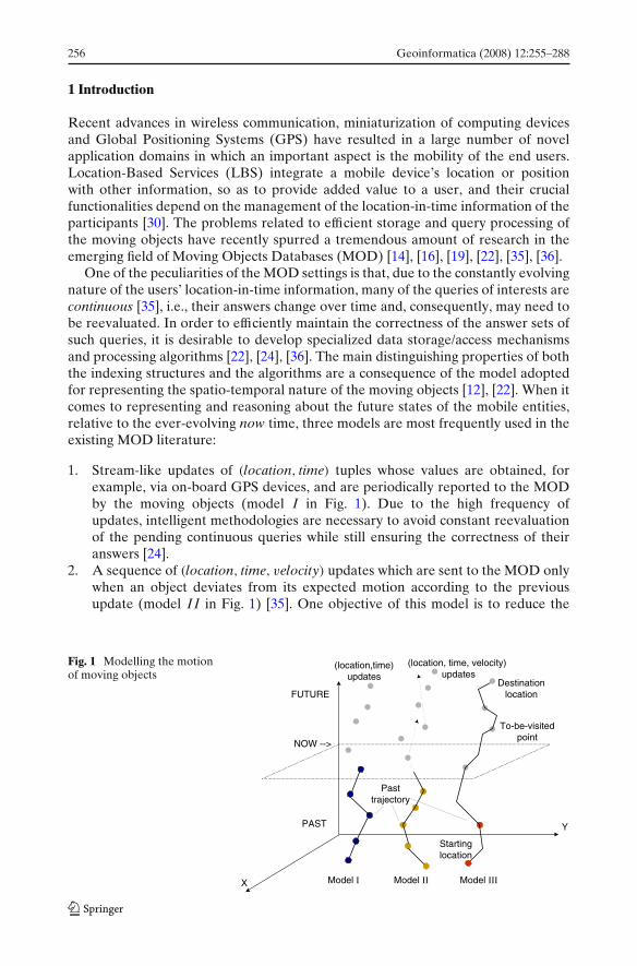
One of the peculiarities of the MOD settings is that, due to the constantly evolvingnature of the users’ location-in-time information, many of the queries of interests arecontinuous [35], i.e., their answers change over time and, consequently, may need tobe reevaluated. In order to efficiently maintain the correctness of the answer sets ofsuch queries, it is desirable to develop specialized data storage/access mechanismsand processing algorithms [22], [24], [36]. The main distinguishing properties of boththe indexing structures and the algorithms are a consequence of the model adoptedfor representing the spatio-temporal nature of the moving objects [12], [22]. When itcomes to representing and reasoning about the future states of the mobile entities,relative to the ever-evolving now time, three models are most frequently used in theexisting MOD literature:

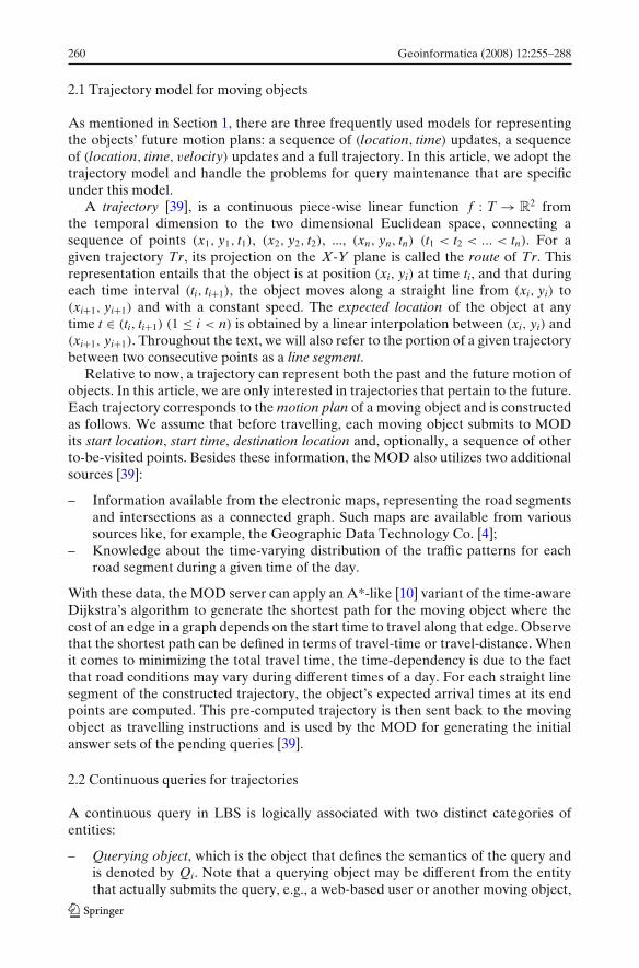
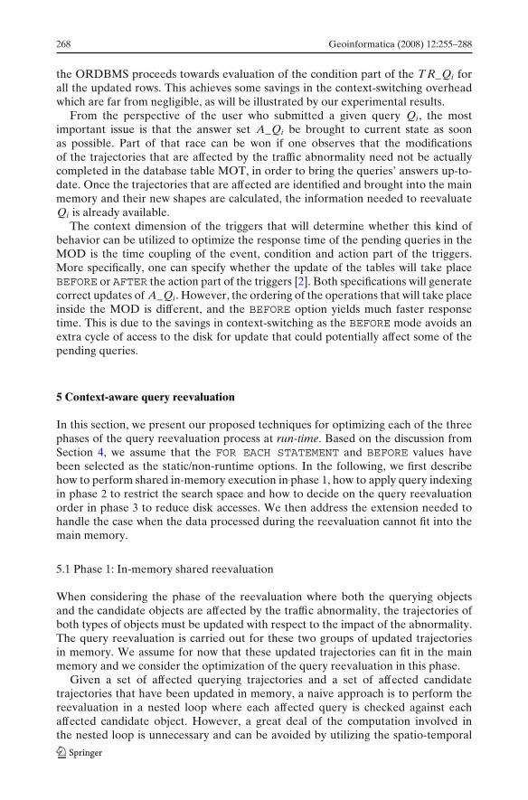
1. Stream-like updates of (location, time) tuples whose values are obtained, forexample, via on-board GPS devices, and are periodically reported to the MODby the moving objects (model I in Fig. 1). Due to the high frequency ofupdates, intelligent methodologies are necessary to avoid constant reevaluationof the pending continuous queries while still ensuring the correctness of theiranswers [24].

2. A sequence of (location, time, velocity) updates which are sent to the MOD onlywhen an object deviates from its expected motion according to the previousupdate (model I I in Fig. 1) [35]. One objective of this model is to reduce the

Fig. 1 Modelling the motionof moving objects

FUTURE

PAST

NOW -->

Y

X

Startinglocation

(location,time)updates

(location, time, velocity) updates

To-be-visitedpoint

Destinationlocation

Pasttrajectory

Model I Model II Model III

Geoinformatica (2008) 12:255–288 257

communication overhead between the moving objects and the server, whileensuring a bounded error on the MOD representation of the objects’ motion [14],[19], [41].

3. A trajectory, which is a sequence of 3D points (x1, y1, t1), (x2, y2, t2), . . .,(xn, yn, tn), (t1 < t2 < . . . < tn), is used to represent the entire future motion planof an object (model I I I in Fig. 1). Between any two consecutive points, the objectis assumed to move along a straight line with a constant speed. This is a realisticmodel for many entities in practical settings when representing future motionplans, e.g., public transportation vehicles, police patrol cars, delivery trucks andindividuals travelling back-and-forth between home and work. Furthermore,many individuals rely on certain online trip planning services, such as Mapquest,Yahoo! Maps and Google Maps,1 to provide driving directions(essentially futuretrajectories). It has been reported by Forbes.com [3] that the number of distinctusers that request future trajectory generation monthly reaches 46.4 million forMapquest, 20 million for Yahoo! Maps and 19.1 million for Google Maps. Adistinguishing feature of the trajectory model is that it enables the MOD toanswer predictive queries pertaining to the locations of the moving objects infuture time intervals, which can be useful for various planning purposes.

Note that when it comes to the past location-in-time information, all three modelsconverge in typical MOD settings, in the sense that the historical data is often storedas trajectories.

1.1 Motivation

In this article we assume that the future motion plans of the moving objects arerepresented as trajectories and consider a problem that is inherent to continuousquery management in such settings, which has not been addressed formally before.Namely, when constructing a trajectory for the future movement of a given object,the MOD relies on certain speed-distribution information regarding the individualroad segments. The MOD constantly manages a large number of such trajectoriesand answers predictive continuous queries like, for example: Q1: retrieve all the mov-ing objects that will be within the Northwestern University campus (sometimes/always)between 4 pm and 5 pm. When an unexpected traffic abnormality happens, e.g., anaccident or a road work, it may affect the future portions of the trajectories passingthrough the abnormality region throughout its duration. This, in turn, affects thecorrectness of the pending continuous queries in a much larger geographic area. Thekey problem is how to efficiently reevaluate such a set of pending queries so thattheir answer sets can be brought up to date with the new traffic conditions.

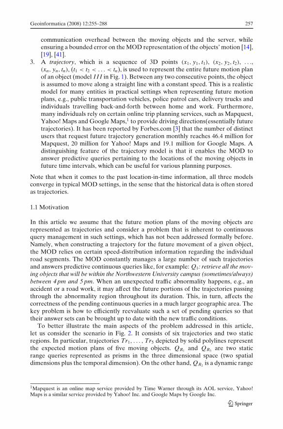
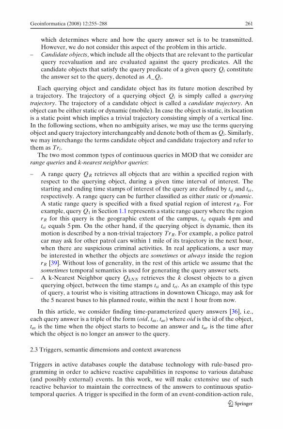
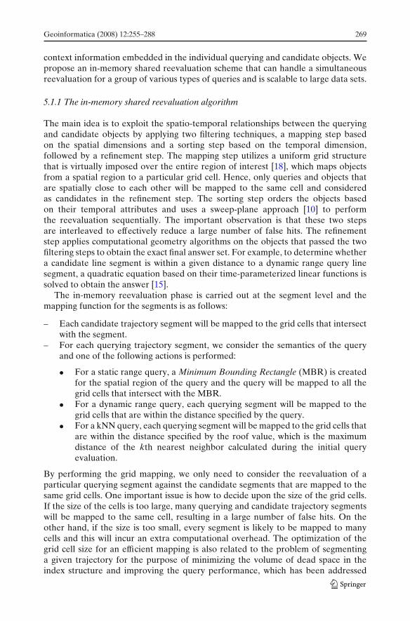
To better illustrate the main aspects of the problem addressed in this article,let us consider the scenario in Fig. 2. It consists of six trajectories and two staticregions. In particular, trajectories Tr1, . . . , Tr5 depicted by solid polylines representthe expected motion plans of five moving objects. QR1 and QR3 are two staticrange queries represented as prisms in the three dimensional space (two spatialdimensions plus the temporal dimension). On the other hand, QR2 is a dynamic range

1Mapquest is an online map service provided by Time Warner through its AOL service, Yahoo!Maps is a similar service provided by Yahoo! Inc. and Google Maps by Google Inc.

258 Geoinformatica (2008) 12:255–288

Tr1 Tr2 Tr3

Tr4

Tr5TIME

Y

X

QR1

QR3

Tr1 Tr2 Tr3

Tr6

Tr4

Tr5TIME

Y

X

QR1

QR3

t1

t2

Tr1'Tr2' Tr3' Tr6?QR1)

a Normal Situation b Traffic Abnormality c Affected Trajectories and Queries

Tr6(QR2)

AT t1

Fig. 2 Trajectories, updates and continuous queries

query defined with respect to trajectory Tr6, its query volume is represented by thetwo sheared cylinders over the time interval of interest (a formal definition of thecontinuous queries will be presented in Section 2).

In this example, we assume that the preliminary query answers have beencomputed and the queries are being monitored until some future time of interest.Suppose an accident occurs at some time t1 on a particular road segment after theinitial answer sets of the queries have been computed (cf. Fig. 2b), which affectsthe traffic patterns in a neighboring region (the base of the shaded cylinder inFig. 2c), and its impact on the traffic persists until time t2 (the top of the shadedcylinder in Fig. 2c). The objects moving through the abnormality zone during thistime period will have to be slowed down from their original expected speed used asa parameter when constructing their trajectories. Hence, the future portions of theaffected trajectories need to be updated, which is the case for Tr1, Tr2, Tr3 and Tr6.As illustrated in Fig. 2c, the dashed lines depict the original trajectories while thesolid lines depict the updated trajectories. Now it becomes obvious that the updatesaffect the answers to the pending queries. First, observe that Tr1 is no longer ananswer to QR1 , but Tr2 becomes an answer to QR1 . In addition, since trajectory Tr6

for query QR2 is delayed by the accident, the whole volume of interest (the twosheared cylinders) changes. Hence, QR2 also needs to be reevaluated, upon whichit turns out that Tr4 is not its answer any more, but Tr3 becomes an answer. Anotherimportant observation is that QR3 does not need to be reevaluated at all, since theaccident has no impact on its answer set. Clearly, it is necessary to reevaluate onlythe affected pending queries upon updating the trajectories. The key issue of efficientmaintenance of these queries is minimizing the cost of various overheads, e.g., diskI/Os, context-switching among processes etc.

1.2 Main contributions

One may observe that the aforementioned query maintenance in MOD exhibits areactive pattern that can be accommodated by the event-condition-action (ECA)rules of active database systems [26], [40], which has been well-studied over thelast decade and implemented in existing commercial Object-Relational DatabaseManagement Systems (ORDBMS). However, a MOD-like functionality that couplesthe reactive behavior with the spatio-temporal data management is still missing. Oneof the main contributions of this work stems from the fact that we demonstrate thata MOD system can be integrated into a traditional ORDBMS, where many benefitsof mature and reliable technologies are readily available.

Geoinformatica (2008) 12:255–288 259

In this article we present an integrated approach towards the optimization of con-tinuous query reevaluation in MOD that covers two popular categories of queries:range queries and k-Nearest Neighbor (kNN) queries, and we create a seamlessframework which facilitates scalable execution when a set of mixed continuousqueries are posed to the system. Upon a detection of an abnormality, we reducethe unnecessary database table accesses and computations for each type of thequery and, moreover, we share the spatio-temporal context information among thequeries to increase the overall efficiency of the reevaluation. As we will demonstrate,further improvements can be achieved when the process of updating the affectedtrajectories is intelligently intermixed with that of updating the answers to thepending continuous queries. For this purpose, we propose a set of specifications forthe triggers that perform the desired reactive behavior along with techniques forordering their execution. Our main goal is to reduce the processing time spent fromthe moment a particular abnormality is presented to the MOD, up to the point whenall the pending continuous queries’ answer sets are brought up-to-date. In summary,the contributions of this article are as follows:

1. We provide a framework for efficiently maintaining continuous queries on futuretrajectories when a subset of them are subject to bulk updates.

2. We identify three distinct phases required for the complete reevaluation ofthe pending queries and propose appropriate techniques that can improve thereevaluation performance in each phase, by intelligently combining the updatesto the trajectories with the updates to the query answers. In particular, we: (a)propose an in-memory shared reevaluation scheme that interleaves mapping onthe spatial dimensions with a sweep-plane approach on the temporal dimensionto avoid unnecessary computation, (b) adapt the query indexing technique to thetrajectory data to limit the search space and (c) utilize ordering based on space-filling curves to improve the I/O efficiency.

3. As a proof of concept, we have fully implemented our system on top of anexisting commercial ORDBMS—Oracle 9i [5].

4. We have conducted an extensive set of experiments to validate our approachand obtained quantitative analysis of the benefits of the proposed optimizationtechniques.

The rest of this article is organized as follows: Section 2 provides an overviewof the problem and reviews the preliminary background. Section 3 presents thearchitecture of our system prototype and explains the essential features of thereevaluation procedures for continuous queries. Section 4 and section 5 elaborateon our optimization techniques and their impact on query reevaluation. Section 6discusses the experimental evaluation results and Section 7 positions our workwith respect to the related literature. Section 8 concludes the article and outlinesdirections for future work.

2 Preliminaries

In this section we formally introduce the trajectory data model and the semanticsof the continuous queries considered in this work. We also examine some of thesemantic dimensions of the triggers in active database systems.

260 Geoinformatica (2008) 12:255–288

2.1 Trajectory model for moving objects

As mentioned in Section 1, there are three frequently used models for representingthe objects’ future motion plans: a sequence of (location, time) updates, a sequenceof (location, time, velocity) updates and a full trajectory. In this article, we adopt thetrajectory model and handle the problems for query maintenance that are specificunder this model.

A trajectory [39], is a continuous piece-wise linear function f : T → R2 from

the temporal dimension to the two dimensional Euclidean space, connecting asequence of points (x1, y1, t1), (x2, y2, t2), ..., (xn, yn, tn) (t1 < t2 < ... < tn). For agiven trajectory Tr, its projection on the X-Y plane is called the route of Tr. Thisrepresentation entails that the object is at position (xi, yi) at time ti, and that duringeach time interval (ti, ti+1), the object moves along a straight line from (xi, yi) to(xi+1, yi+1) and with a constant speed. The expected location of the object at anytime t ∈ (ti, ti+1) (1 ≤ i < n) is obtained by a linear interpolation between (xi, yi) and(xi+1, yi+1). Throughout the text, we will also refer to the portion of a given trajectorybetween two consecutive points as a line segment.

Relative to now, a trajectory can represent both the past and the future motion ofobjects. In this article, we are only interested in trajectories that pertain to the future.Each trajectory corresponds to the motion plan of a moving object and is constructedas follows. We assume that before travelling, each moving object submits to MODits start location, start time, destination location and, optionally, a sequence of otherto-be-visited points. Besides these information, the MOD also utilizes two additionalsources [39]:

– Information available from the electronic maps, representing the road segmentsand intersections as a connected graph. Such maps are available from varioussources like, for example, the Geographic Data Technology Co. [4];

– Knowledge about the time-varying distribution of the traffic patterns for eachroad segment during a given time of the day.

With these data, the MOD server can apply an A*-like [10] variant of the time-awareDijkstra’s algorithm to generate the shortest path for the moving object where thecost of an edge in a graph depends on the start time to travel along that edge. Observethat the shortest path can be defined in terms of travel-time or travel-distance. Whenit comes to minimizing the total travel time, the time-dependency is due to the factthat road conditions may vary during different times of a day. For each straight linesegment of the constructed trajectory, the object’s expected arrival times at its endpoints are computed. This pre-computed trajectory is then sent back to the movingobject as travelling instructions and is used by the MOD for generating the initialanswer sets of the pending queries [39].

2.2 Continuous queries for trajectories

A continuous query in LBS is logically associated with two distinct categories ofentities:

– Querying object, which is the object that defines the semantics of the query andis denoted by Qi. Note that a querying object may be different from the entitythat actually submits the query, e.g., a web-based user or another moving object,

Geoinformatica (2008) 12:255–288 261

which determines where and how the query answer set is to be transmitted.However, we do not consider this aspect of the problem in this article.

– Candidate objects, which include all the objects that are relevant to the particularquery reevaluation and are evaluated against the query predicates. All thecandidate objects that satisfy the query predicate of a given query Qi constitutethe answer set to the query, denoted as A_Qi.

Each querying object and candidate object has its future motion described bya trajectory. The trajectory of a querying object Qi is simply called a queryingtrajectory. The trajectory of a candidate object is called a candidate trajectory. Anobject can be either static or dynamic (mobile). In case the object is static, its locationis a static point which implies a trivial trajectory consisting simply of a vertical line.In the following sections, when no ambiguity arises, we may use the terms queryingobject and query trajectory interchangeably and denote both of them as Qi. Similarly,we may interchange the terms candidate object and candidate trajectory and refer tothem as Tri.

The two most common types of continuous queries in MOD that we consider arerange queries and k-nearest neighbor queries:

– A range query QR retrieves all objects that are within a specified region withrespect to the querying object, during a given time interval of interest. Thestarting and ending time stamps of interest of the query are defined by tsi and tei,respectively. A range query can be further classified as either static or dynamic.A static range query is specified with a fixed spatial region of interest rR. Forexample, query Q1 in Section 1.1 represents a static range query where the regionrR for this query is the geographic extent of the campus, tsi equals 4 pm andtei equals 5 pm. On the other hand, if the querying object is dynamic, then itsmotion is described by a non-trivial trajectory TrR. For example, a police patrolcar may ask for other patrol cars within 1 mile of its trajectory in the next hour,when there are suspicious criminal activities. In real applications, a user maybe interested in whether the objects are sometimes or always inside the regionrR [39]. Without loss of generality, in the rest of this article we assume that thesometimes temporal semantics is used for generating the query answer sets.

– A k-Nearest Neighbor query QkNN retrieves the k closest objects to a givenquerying object, between the time stamps tsi and tei. As an example of this typeof query, a tourist who is visiting attractions in downtown Chicago, may ask forthe 5 nearest buses to his planned route, within the next 1 hour from now.

In this article, we consider finding time-parameterized query answers [36], i.e.,each query answer is a triple of the form (oid, tas, tae) where oid is the id of the object,tas is the time when the object starts to become an answer and tae is the time afterwhich the object is no longer an answer to the query.

2.3 Triggers, semantic dimensions and context awareness

Triggers in active databases couple the database technology with rule-based pro-gramming in order to achieve reactive capabilities in response to various database(and possibly external) events. In this work, we will make extensive use of suchreactive behavior to maintain the correctness of the answers to continuous spatio-temporal queries. A trigger is specified in the form of an event-condition-action rule,

262 Geoinformatica (2008) 12:255–288

which stipulates that an action will be executed upon the occurrence of a particularevent, provided that a given condition holds [2]. One of the early observations inthe active database literature [13], [26] was that in many prototype systems, triggerswith similar specifications were exhibiting different executional behavior. In orderto better categorize the declarative aspects of the triggers’ specifications and enablemore precise reasoning about their behavior, researchers have identified a numberof so-called semantic dimensions and a set of values that may be chosen for eachdimension, many of which have become part of the latest SQL standard [2]. Forexample, one semantic dimension is the granularity of updates: upon detection ofcertain event, the reaction of the ORDBMS can be in a per-tuple manner, i.e., exe-cute the action part of the trigger for each individual tuple that has been modified,or per-set manner, i.e., execute the action only once for the entire set of the modifiedtuples. As another example, one can specify different coupling modes: e.g., should thecondition evaluation immediately follow the detection of the event, or should it bedeferred until the end of the current transaction. A total of 13 different semantic di-mensions have been identified in [13], and later in the corresponding sections we willelaborate in detail on the semantic dimensions of the triggers that we use in this work.

Analogous to trigger semantic dimensions, we can also speak of query semanticdimensions. These include the motion patterns of queries (dynamic or static), seman-tics of query predicates (range or kNN), locations of queries, spatio-temporal extentsof queries, etc. Together with the semantic dimensions of the triggers, the correlationamong these context dimensions can highly impact the efficiency of the reevaluationand should be orchestrated to obtain further performance gains. The values of someof these dimensions can be determined at specification time, whereas the others needto be determined at run-time. In subsequent sections we will discuss how to decidethe best values for these semantic dimensions to improve the performance of querymaintenance.

3 Trajectory processing of continuous queries

The trajectory model, when applicable, alleviates the problem of frequent updatesto the MOD and enables currently available answers for spatio-temporal querieswhich pertain to any future time interval. However, as we discussed in Section 1,the main problem here is due to the fact that the changes to the motion plans ofindividual objects, which may occur at any time between requesting an answer setto a particular query from the MOD and the end time of interest for that query inthe future, could change the initially calculated answer set. This raises the questionof how to maintain efficiently the answer sets to the queries on trajectories againstchanges to the future motion plans of the moving objects. In this section, we firstdiscuss the relevant aspects of the reactive behavior of MOD, then introduce theoverall architecture of our system. Based on these we outline the basic procedureand methodology for maintaining continuous queries.

3.1 Reactive query maintenance

Once the MOD server receives a request for processing a new query, its interfaceextracts the elements of the query syntax necessary for query maintenance, e.g.,

Geoinformatica (2008) 12:255–288 263

tei (end time of interest) that specifies the time after which the query no longerneeds to be monitored and can be purged from the system. The basic paradigm formaintaining the answer set to a given continuous query can be described as follows:

1. Upon receiving a new query Qnew, process Qnew and set its answer set A_Qnew;2. Transmit A_Qnew to the user who posed the query;3. Create a trigger T R_Qnew of the form:

EVENT: on update to MODCONDITION: if A_Qnew affectedACTION: reevaluate Qnew and update A_Qnew

In terms of the actual execution model, the step of checking if A_Qnew wasaffected requires reevaluating the query on the modified trajectories. A_Qnew issubsequently updated with the new results, and the user is notified of the changes.

Since we assume that the sources for the reactive behavior are bulk updates to thetrajectory data in the database, we also set up a trigger T R_T AT that continuouslymonitors for any new traffic abnormality:

EVENT: on insert/update of a new traffic abnormality eventCONDITION: if a moving object trajectory Tr is affectedACTION: update Tr to reflect the traffic abnormality

The problem of spatio-temporal query processing on trajectories for the purposeof generating the initial answer set has already been addressed in the literature [16],[22], [23] and is not the main topic of this work. Our objective is to reduce theprocessing time spent from the moment a particular abnormality is presented tothe MOD up to the point when all the pending continuous queries’ answer setsare brought up-to-date. Towards this goal, we focus on orchestrating the executionof the respective triggers, based on intelligent usage of the dependencies amongvarious context/semantic dimensions. When applicable our system also interleavesthe evaluation of condition parts and the execution of action parts of differenttriggers, in order to reduce the overall response time.

3.2 System architecture

The main components of our system are depicted in Fig. 3:

– Moving Object Table (MOT) stores information about the moving objects: theirspatio-temporal trajectories plus some other non-spatial attributes of interestsuch as name, license plate number, model etc. The main attribute traj_shapeis a User Defined Type (UDT) [2] conforming to the object-relational model. Itcontains a handle to the actual trajectory coordinates. The actual trajectoriesare stored as Large Object (LOB) data [2] outside the MOT and can beaccessed via the handles in the respective tuples of the table. More specifically,every trajectory is uniformly split into a number of sub-trajectories, each ofwhich contains a fixed number of line segments, and these sub-trajectories areorganized as a linked list. The handle in the MOT table points to the firstsub-trajectory of the trajectory, from which the entire trajectory can be visitedfollowing the subsequent links. A spatio-temporal variant of the R-tree [17]index such as the STR tree or TB-tree [28], [16] is created on the set of

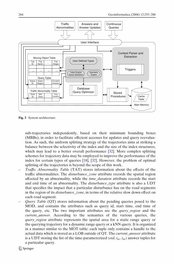
264 Geoinformatica (2008) 12:255–288

Stored Procedures

Main Memory

CacheTable

Moving Object Table

Answers andAnswer Updates

TrafficAbnormalities

ContinuousQueries

Dist.Zone

ZoneID

... TimeDuration

Traffic Abnormality Table

QueryRegion

QueryID

...CurrentAnswer

Query Table

TrajName

...Traj

Shape

... ... ... ...

TrajID

DatabaseQuery Optimizer

User Defined Types

Index EngineQuery Operators

GeometryEngine

Triggers

Context Parser andExtraction

User Interface

Fig. 3 System architecture

sub-trajectories independently, based on their minimum bounding boxes(MBBs), in order to facilitate efficient accesses for updates and query reevalua-tion. As such, the uniform splitting strategy of the trajectories aims at striking abalance between the selectivity of the index and the size of the index structures,which may lead to a better overall performance [32]. More complex splittingschemes for trajectory data may be employed to improve the performance of theindex for certain types of queries [18], [32]. However, the problem of optimalsplitting of the trajectories is beyond the scope of this work.

– Traffic Abnormality Table (TAT) stores information about the effects of thetraffic abnormalities. The disturbance_zone attribute records the spatial regionaffected by an abnormality, while the time_duration attribute records the startand end time of an abnormality. The disturbance_type attribute is also a UDTthat specifies the impact that a particular disturbance has on the road segmentsin the region of its disturbance_zone, in terms of the relative slow down effect oneach road segment.

– Query Table (QT) stores information about the pending queries posed to theMOD, and contains the attributes such as query id, start time, end time ofthe query, etc. The two important attributes are the query_region and thecurrent_answer. According to the semantics of the various queries, thequery_region attribute represents the spatial area for a static range query orthe querying trajectory for a dynamic range query or a kNN query. It is organizedin a manner similar to the MOT table: each tuple only contains a handle to theactual data which is stored as a LOB outside of QT. The current_answer attributeis a UDT storing the list of the time-parameterized (oid, tas, tae) answer tuples fora particular query.

Geoinformatica (2008) 12:255–288 265

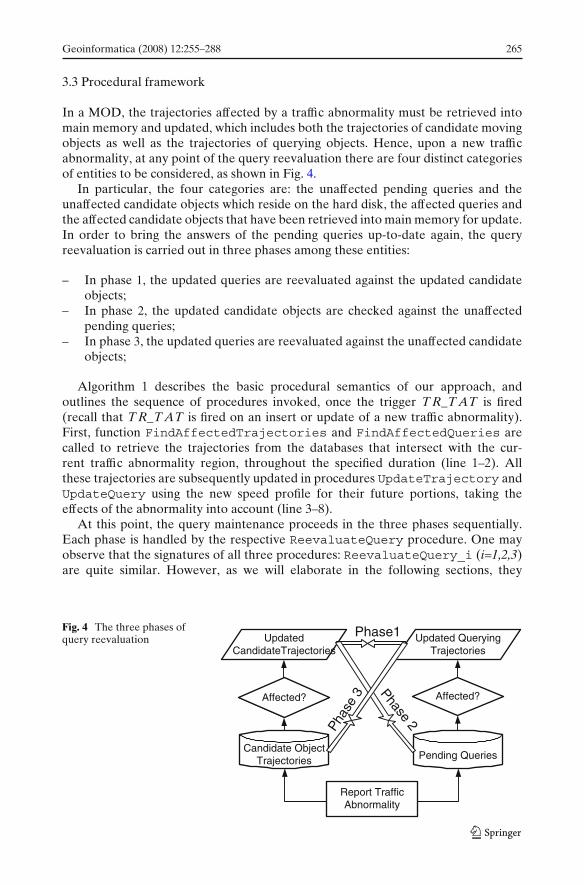
3.3 Procedural framework

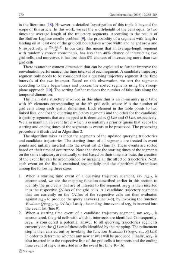
In a MOD, the trajectories affected by a traffic abnormality must be retrieved intomain memory and updated, which includes both the trajectories of candidate movingobjects as well as the trajectories of querying objects. Hence, upon a new trafficabnormality, at any point of the query reevaluation there are four distinct categoriesof entities to be considered, as shown in Fig. 4.

In particular, the four categories are: the unaffected pending queries and theunaffected candidate objects which reside on the hard disk, the affected queries andthe affected candidate objects that have been retrieved into main memory for update.In order to bring the answers of the pending queries up-to-date again, the queryreevaluation is carried out in three phases among these entities:

– In phase 1, the updated queries are reevaluated against the updated candidateobjects;

– In phase 2, the updated candidate objects are checked against the unaffectedpending queries;

– In phase 3, the updated queries are reevaluated against the unaffected candidateobjects;

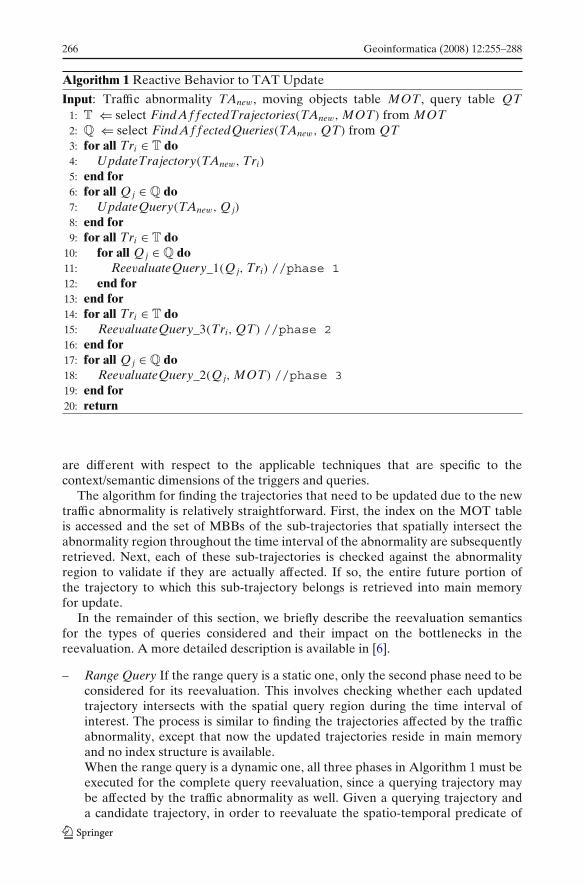
Algorithm 1 describes the basic procedural semantics of our approach, andoutlines the sequence of procedures invoked, once the trigger T R_T AT is fired(recall that T R_T AT is fired on an insert or update of a new traffic abnormality).First, function FindAffectedTrajectories and FindAffectedQueries arecalled to retrieve the trajectories from the databases that intersect with the cur-rent traffic abnormality region, throughout the specified duration (line 1–2). Allthese trajectories are subsequently updated in procedures UpdateTrajectory andUpdateQuery using the new speed profile for their future portions, taking theeffects of the abnormality into account (line 3–8).

At this point, the query maintenance proceeds in the three phases sequentially.Each phase is handled by the respective ReevaluateQuery procedure. One mayobserve that the signatures of all three procedures: ReevaluateQuery_i (i=1,2,3)are quite similar. However, as we will elaborate in the following sections, they

Fig. 4 The three phases ofquery reevaluation

Phase1

Phas

e 3

Report TrafficAbnormality

Candidate ObjectTrajectories Pending Queries

UpdatedCandidateTrajectories

Affected?

Updated QueryingTrajectories

Affected?Phase 2

266 Geoinformatica (2008) 12:255–288

Algorithm 1 Reactive Behavior to TAT Update

Input: Traffic abnormality TAnew, moving objects table MOT, query table QT1: T ⇐ select FindAf f ectedTrajectories(TAnew, MOT) from MOT2: Q ⇐ select FindAf f ectedQueries(TAnew, QT) from QT3: for all Tri ∈ T do4: UpdateTrajectory(TAnew, Tri)

5: end for6: for all Q j ∈ Q do7: UpdateQuery(TAnew, Q j)

8: end for9: for all Tri ∈ T do

10: for all Q j ∈ Q do11: ReevaluateQuery_1(Q j, Tri) //phase 112: end for13: end for14: for all Tri ∈ T do15: ReevaluateQuery_3(Tri, QT) //phase 216: end for17: for all Q j ∈ Q do18: ReevaluateQuery_2(Q j, MOT) //phase 319: end for20: return

are different with respect to the applicable techniques that are specific to thecontext/semantic dimensions of the triggers and queries.

The algorithm for finding the trajectories that need to be updated due to the newtraffic abnormality is relatively straightforward. First, the index on the MOT tableis accessed and the set of MBBs of the sub-trajectories that spatially intersect theabnormality region throughout the time interval of the abnormality are subsequentlyretrieved. Next, each of these sub-trajectories is checked against the abnormalityregion to validate if they are actually affected. If so, the entire future portion ofthe trajectory to which this sub-trajectory belongs is retrieved into main memoryfor update.

In the remainder of this section, we briefly describe the reevaluation semanticsfor the types of queries considered and their impact on the bottlenecks in thereevaluation. A more detailed description is available in [6].

– Range Query If the range query is a static one, only the second phase need to beconsidered for its reevaluation. This involves checking whether each updatedtrajectory intersects with the spatial query region during the time interval ofinterest. The process is similar to finding the trajectories affected by the trafficabnormality, except that now the updated trajectories reside in main memoryand no index structure is available.When the range query is a dynamic one, all three phases in Algorithm 1 must beexecuted for the complete query reevaluation, since a querying trajectory maybe affected by the traffic abnormality as well. Given a querying trajectory anda candidate trajectory, in order to reevaluate the spatio-temporal predicate of

Geoinformatica (2008) 12:255–288 267

the query, the two trajectories need to be broken down into segments and thecalculation is performed at the line segments level using the linear functions ofthe segments [23].

– kNN Query Similar to dynamic range queries, kNN queries are reevaluated atthe line segments level. The main difference is that for each kNN query, we mustcheck the current answer set list against every new candidate object. To reducethe number of comparisons made, we adopt the idea of windowing the kNNquery [19] by maintaining a roof value for each querying trajectory segment,which is obtained during the initial query evaluation. The roof value is themaximum distance of the kth nearest neighbor to that line segment. It minimizesthe number of candidate trajectories/segments that need to be examined inorder to find out the answer set of the kNN query. During the reevaluation, weretrieve the candidate segments which are within roof distance of the queryingsegment. In case we cannot find enough nearest neighbors within the retrieveddata, we increase the roof value by certain percentage to retrieve more candi-date segments. This iteration continues until we have completely updated theanswer set.

4 System-level context-aware optimization

In this section, we present our static optimization techniques at the system level, i.e.,how to select the proper values for the respective semantic dimensions of the triggersto minimize the context-switching overhead.

One of the semantic dimensions that may have different values in a particulartrigger is the granularity of execution, i.e., whether to execute the action partof the trigger at set level or at instance level [26]. Recall from our discussion inSection 2.3, to achieve the behavior corresponding to the values of update granularityoptions, generally one needs to use one of the clauses: FOR EACH ROW or FOR EACHSTATEMENT respectively in the specification of T R_Qi [2].

If the executional granularity specified is at instance level, whenever a particulartrajectory Tr j is updated, the corresponding instance of T R_Qi will evaluate itagainst Qi, in order to check if the modifications to Tr j affect the answer set A_Qi.If so, A_Qi will be updated accordingly. This cycle will be repeated for each of thesubsequent trajectories that are affected by the update to the TAT. However, at eachcycle, we have at least three major context-switchings that the ORDBMS2 needs todo, and these will be reflected at the Operating System level:

1. From the update mode of MOT to checking if A_Qi is affected;2. From checking if A_Qi is affected to eventually updating the answer set;3. From updating A_Qi, back to the update mode of MOT for processing and

completing the modification to another trajectory Trk.

On the other hand, if T R_Qi is specified to execute at the set level, all the tra-jectories affected by the traffic abnormality will be updated in the MOT first before

2The specification of the SQL99 standard distinguishes between statement execution context, routineexecution context, and trigger execution context [2].

268 Geoinformatica (2008) 12:255–288

the ORDBMS proceeds towards evaluation of the condition part of the T R_Qi forall the updated rows. This achieves some savings in the context-switching overheadwhich are far from negligible, as will be illustrated by our experimental results.

From the perspective of the user who submitted a given query Qi, the mostimportant issue is that the answer set A_Qi be brought to current state as soonas possible. Part of that race can be won if one observes that the modificationsof the trajectories that are affected by the traffic abnormality need not be actuallycompleted in the database table MOT, in order to bring the queries’ answers up-to-date. Once the trajectories that are affected are identified and brought into the mainmemory and their new shapes are calculated, the information needed to reevaluateQi is already available.

The context dimension of the triggers that will determine whether this kind ofbehavior can be utilized to optimize the response time of the pending queries in theMOD is the time coupling of the event, condition and action part of the triggers.More specifically, one can specify whether the update of the tables will take placeBEFORE or AFTER the action part of the triggers [2]. Both specifications will generatecorrect updates of A_Qi. However, the ordering of the operations that will take placeinside the MOD is different, and the BEFORE option yields much faster responsetime. This is due to the savings in context-switching as the BEFORE mode avoids anextra cycle of access to the disk for update that could potentially affect some of thepending queries.

5 Context-aware query reevaluation

In this section, we present our proposed techniques for optimizing each of the threephases of the query reevaluation process at run-time. Based on the discussion fromSection 4, we assume that the FOR EACH STATEMENT and BEFORE values havebeen selected as the static/non-runtime options. In the following, we first describehow to perform shared in-memory execution in phase 1, how to apply query indexingin phase 2 to restrict the search space and how to decide on the query reevaluationorder in phase 3 to reduce disk accesses. We then address the extension needed tohandle the case when the data processed during the reevaluation cannot fit into themain memory.

5.1 Phase 1: In-memory shared reevaluation

When considering the phase of the reevaluation where both the querying objectsand the candidate objects are affected by the traffic abnormality, the trajectories ofboth types of objects must be updated with respect to the impact of the abnormality.The query reevaluation is carried out for these two groups of updated trajectoriesin memory. We assume for now that these updated trajectories can fit in the mainmemory and we consider the optimization of the query reevaluation in this phase.

Given a set of affected querying trajectories and a set of affected candidatetrajectories that have been updated in memory, a naive approach is to perform thereevaluation in a nested loop where each affected query is checked against eachaffected candidate object. However, a great deal of the computation involved inthe nested loop is unnecessary and can be avoided by utilizing the spatio-temporal

Geoinformatica (2008) 12:255–288 269

context information embedded in the individual querying and candidate objects. Wepropose an in-memory shared reevaluation scheme that can handle a simultaneousreevaluation for a group of various types of queries and is scalable to large data sets.

5.1.1 The in-memory shared reevaluation algorithm

The main idea is to exploit the spatio-temporal relationships between the queryingand candidate objects by applying two filtering techniques, a mapping step basedon the spatial dimensions and a sorting step based on the temporal dimension,followed by a refinement step. The mapping step utilizes a uniform grid structurethat is virtually imposed over the entire region of interest [18], which maps objectsfrom a spatial region to a particular grid cell. Hence, only queries and objects thatare spatially close to each other will be mapped to the same cell and consideredas candidates in the refinement step. The sorting step orders the objects basedon their temporal attributes and uses a sweep-plane approach [10] to performthe reevaluation sequentially. The important observation is that these two stepsare interleaved to effectively reduce a large number of false hits. The refinementstep applies computational geometry algorithms on the objects that passed the twofiltering steps to obtain the exact final answer set. For example, to determine whethera candidate line segment is within a given distance to a dynamic range query linesegment, a quadratic equation based on their time-parameterized linear functions issolved to obtain the answer [15].

The in-memory reevaluation phase is carried out at the segment level and themapping function for the segments is as follows:

– Each candidate trajectory segment will be mapped to the grid cells that intersectwith the segment.

– For each querying trajectory segment, we consider the semantics of the queryand one of the following actions is performed:

• For a static range query, a Minimum Bounding Rectangle (MBR) is createdfor the spatial region of the query and the query will be mapped to all thegrid cells that intersect with the MBR.

• For a dynamic range query, each querying segment will be mapped to thegrid cells that are within the distance specified by the query.

• For a kNN query, each querying segment will be mapped to the grid cells thatare within the distance specified by the roof value, which is the maximumdistance of the kth nearest neighbor calculated during the initial queryevaluation.

By performing the grid mapping, we only need to consider the reevaluation of aparticular querying segment against the candidate segments that are mapped to thesame grid cells. One important issue is how to decide upon the size of the grid cells.If the size of the cells is too large, many querying and candidate trajectory segmentswill be mapped to the same cell, resulting in a large number of false hits. On theother hand, if the size is too small, every segment is likely to be mapped to manycells and this will incur an extra computational overhead. The optimization of thegrid cell size for an efficient mapping is also related to the problem of segmentinga given trajectory for the purpose of minimizing the volume of dead space in theindex structure and improving the query performance, which has been addressed

270 Geoinformatica (2008) 12:255–288

in the literature [18]. However, a detailed investigation of this topic is beyond thescope of this article. In this work, we set the width/height of the cells equal to twotimes the average length of the trajectory segments. According to the results ofthe Buffon–Laplace needle problem [9], the probability of a segment with length llanding on at least one of the grid cell boundaries whose width and height are a andb respectively, is 2l(a+b)−l2

πab . In our case, this means that an average-length segmentwith randomly chosen coordinates, has less than 48% chance of intersecting twogrid cells, and moreover, it has less than 8% chances of intersecting more than twogrid cells.

There is another context dimension that can be exploited to further improve thereevaluation performance: the time interval of each segment. A candidate trajectorysegment only needs to be considered for a querying trajectory segment if the timeintervals of the two intersect. Based on this observation, we sort the segmentsaccording to their begin times and process the sorted segments using the sweep-plane approach [10]. The sorting further reduces the number of false hits along thetemporal dimension.

The main data structure involved in this algorithm is an in-memory grid tablewith N2 elements corresponding to the N2 grid cells, where N is the number ofgrid cells along each spatial dimension. Each element in the table points to twolinked lists, one for the querying trajectory segments and the other for the candidatetrajectory segments that are mapped to it, denoted as QList and OList, respectively.We also maintain an event list E which is essentially a priority queue that keeps thestarting and ending times of the segments as events to be processed. The processingprocedure is illustrated in Algorithm 2.

The algorithm takes as input the segments of the updated querying trajectoriesand candidate trajectories. The starting times of all segments are treated as eventpoints and initially inserted into the event list E (line 1). These events are sortedbased on their time of occurrence. Note that since the starting times of the segmentson the same trajectory are naturally sorted based on their time attribute, the creationof the event list can be accomplished by merging all the affected trajectories. Next,each event on the list is examined sequentially and the algorithm differentiatesamong the following three cases:

1. When a starting time event of a querying trajectory segment, say segQ, isencountered, we use the mapping function described earlier in this section toidentify the grid cells that are of interest to the segment. segQ is then insertedinto the respective QLists of the grid cells. All candidate trajectory segmentsthat are currently on the OLists of the respective cells are then evaluatedagainst segQ to produce the query answers (line 3–8), by invoking the functionEvaluateQ(segQ, cij.OList). Lastly, the ending time event of segQ is inserted intothe event list (line 9).

2. When a starting time event of a candidate trajectory segment, say segTr, isencountered, the grid cells with which it intersects are identified. Consequently,segTr is considered a potential answer to all querying trajectories segmentscurrently on the QLists of those cells identified by the mapping. The refinementstep is then carried out by invoking the function EvaluateTr(segTr, cmn.QList)in order to determine whether any new answer will be produced. Finally, segTr isalso inserted into the respective lists of the grid cells it intersects and the endingtime event of segTr is inserted into the event list (line 10–16).

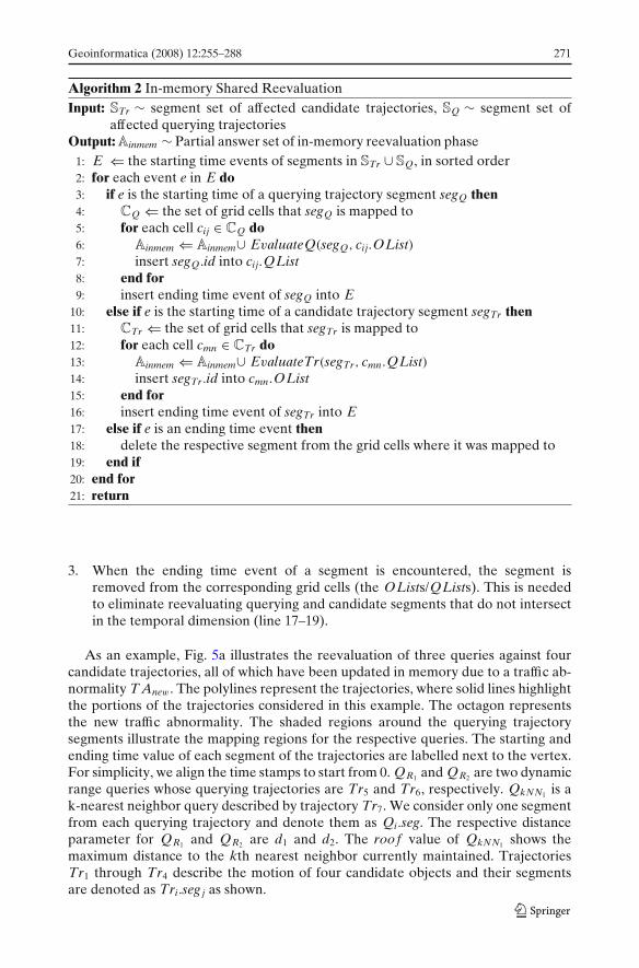
Geoinformatica (2008) 12:255–288 271

Algorithm 2 In-memory Shared ReevaluationInput: STr ∼ segment set of affected candidate trajectories, SQ ∼ segment set of

affected querying trajectoriesOutput: Ainmem ∼ Partial answer set of in-memory reevaluation phase

1: E ⇐ the starting time events of segments in STr ∪ SQ, in sorted order2: for each event e in E do3: if e is the starting time of a querying trajectory segment segQ then4: CQ ⇐ the set of grid cells that segQ is mapped to5: for each cell cij ∈ CQ do6: Ainmem ⇐ Ainmem∪ EvaluateQ(segQ, cij.OList)7: insert segQ.id into cij.QList8: end for9: insert ending time event of segQ into E

10: else if e is the starting time of a candidate trajectory segment segTr then11: CTr ⇐ the set of grid cells that segTr is mapped to12: for each cell cmn ∈ CTr do13: Ainmem ⇐ Ainmem∪ EvaluateTr(segTr, cmn.QList)14: insert segTr.id into cmn.OList15: end for16: insert ending time event of segTr into E17: else if e is an ending time event then18: delete the respective segment from the grid cells where it was mapped to19: end if20: end for21: return

3. When the ending time event of a segment is encountered, the segment isremoved from the corresponding grid cells (the OLists/QLists). This is neededto eliminate reevaluating querying and candidate segments that do not intersectin the temporal dimension (line 17–19).

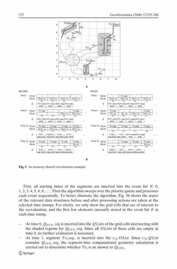
As an example, Fig. 5a illustrates the reevaluation of three queries against fourcandidate trajectories, all of which have been updated in memory due to a traffic ab-normality T Anew. The polylines represent the trajectories, where solid lines highlightthe portions of the trajectories considered in this example. The octagon representsthe new traffic abnormality. The shaded regions around the querying trajectorysegments illustrate the mapping regions for the respective queries. The starting andending time value of each segment of the trajectories are labelled next to the vertex.For simplicity, we align the time stamps to start from 0. QR1 and QR2 are two dynamicrange queries whose querying trajectories are Tr5 and Tr6, respectively. QkNN1 is ak-nearest neighbor query described by trajectory Tr7. We consider only one segmentfrom each querying trajectory and denote them as Qi.seg. The respective distanceparameter for QR1 and QR2 are d1 and d2. The roof value of QkNN1 shows themaximum distance to the kth nearest neighbor currently maintained. TrajectoriesTr1 through Tr4 describe the motion of four candidate objects and their segmentsare denoted as Tri.seg j as shown.

272 Geoinformatica (2008) 12:255–288

Tr5 (QR1)

Tr7 (QkNN1)

Tr1

Tr2

Tr3 Tr4

2 5

10

11

16 20

2515

4

12

0

10

1

6

12

21

1 4 62 3 5 7 8

a

b

c

d

e

f

g

hTr6(QR2)

3

8

seg1seg2

seg1

seg1

seg2

seg3

seg1

seg2

seg3

TAnew

11

a

Time 3

Time 10

Time 12

c4bc4a

OList:QList:

Tr1.seg1

---

c6d

-QkNN1.seg

c7d

Tr4.seg1

QkNN1.seg...

c7ec7d

OList:QList:

Tr4.seg2

QkNN1.seg

Tr4.seg2

QkNN1.seg

c7fc6e

OList:QList:

Tr2.seg1

-Tr4.seg2

-

c7f

Tr4.seg2

QkNN1.seg...

...

Time 1

c6d

OList:QList:

-QkNN1.seg

c7d

-QkNN1.seg

c6e

-QkNN1.seg

...

E

E

E

E

...

-QkNN1.seg

c7e

1(Tr4.seg1

start)2(Tr1.seg1

start)3(QR1.seg

start)4(Tr2.seg1

start)

...

...

...

3(QR1.segstart)

4(Tr2.seg1

start)5(Tr1.seg1

end)5(Tr1.seg2

start)

Tr2.seg1

QkNN1.seg

c6e

10(Tr1.seg2 end)

10(QkNN1.seg end)

11(QR2.seg start)

11(Tr3.seg1 start)

12(Tr2.seg1 end)

12(Tr4.seg2 end)

12(Tr4.seg3 start)

15(QR2.seg end)

Time 3

Time 10

Time 12

c4bc4a

OList:QList:

Tr1.seg1

QR1.seg

-QR1.seg

c6d

-QkNN1.seg

c7d

Tr4.seg1

QkNN1.seg...

c7ec7d

OList:QList:

Tr4.seg2

-

Tr4.seg2

-

OList:QList:

c7f

Tr4.seg2

-...

Time 1

c6d

OList:QList:

-QkNN1.seg

c7d

Tr4.seg1

QkNN1.seg

c6e

-QkNN1.seg

...

E

E

E

E

...

-QkNN1.seg

c7e

2(Tr1.seg1

start)3(QR1.seg

start)4(Tr2.seg1

start)5(Tr1.seg2

start)

...

...

...

4(Tr2.seg1

start)5(Tr1.seg1

end)5(Tr1.seg2

start)6(Tr4.seg1

end)

Tr2.seg1

-c6e

11(QR2.seg start)

11(Tr3.seg1 start)

12(Tr2.seg1

end)12(Tr4.seg2

end)

15(QR2.seg end)

16(Tr3.seg1 end)

16(Tr3.seg2 start)

20(Tr3. seg3 start)

BEFORE AFTER

c2gc2f

Tr3.seg1

-Tr3.seg1

QR2.seg

c7fc6e

--

Tr4.seg3

-c2gc2f

Tr3.seg1

-Tr3.seg1

QR2.seg

...

b

Fig. 5 In-memory shared reevaluation example

First, all starting times of the segments are inserted into the event list E: 0,1, 2, 3, 4, 5, 6, 8, . . .. Then the algorithm sweeps over the priority queue and processeseach event sequentially. To better illustrate the algorithm, Fig. 5b shows the statesof the relevant data structures before and after processing actions are taken at theselected time stamps. For clarity, we only show the grid cells that are of interest tothe reevaluation, and the first few elements currently stored in the event list E ateach time stamp.

– At time 0, QkNN1 .seg is inserted into the QLists of the grid cells intersecting withthe shaded regions for QkNN1 .seg. Since all OLists of these cells are empty attime 0, no further evaluation is necessary.

– At time 1, segment Tr4.seg1 is inserted into the c7d.OList. Since c7d.QListcontains QkNN1 .seg, the segment-wise computational geometry calculation iscarried out to determine whether Tr4 is an answer to QkNN1 .

Geoinformatica (2008) 12:255–288 273

– At time 3 QR1 .seg is inserted into the QLists for grid cell c4a, c4b . At this timeTr1.seg1 is in c4a.OList, thus it is evaluated against QR1 . Note also that the endingtime event for Tr1.seg1 has already been inserted into E.

– At time 10, QkNN1 .seg and Tr1.seg2 (not shown) are removed from their respec-tive grid cells (QLists/OLists).

– At time 12, Tr2.seg1 and Tr4.seg2 are removed from the OLists of the inter-secting cells. Tr4.seg3 is mapped to c7 f .OList and c8 f .OList. However, sinceQkNN1 .seg has been removed from c7 f .QList at time 10, no further reevaluationis needed.

– Finally, the algorithm stops at time stamp 25 when the event list E becomesempty.

To determine the time complexity of Algorithm 2, observe that when initiallycreating the event list in which the segments are sorted according to their startingtime stamps, the total cost is linear in the total number of segments since eachindividual trajectory already has its segments sorted. Let k denote the number ofquerying trajectory segments and let n denote the number of candidate trajectorysegments, the worst case complexity of Algorithm 2 is bounded by O(kn). In practice,however, one may expect a better bound because as a consequence of the sortingof the segments and the mapping of the segments into the grid cells (which is alsolinear in the number of segments), the pairwise evaluation of many segments will beavoided.

5.2 Phase 2: Selecting the relevant subset of triggers

In phase 2, we need to reevaluate the updated moving object trajectories that arein the main memory against the unaffected queries that are on the hard disk. Letus recall our example from Section 2: query QR3 did not need to be reevaluatedsince none of the trajectories in A_QR3 were affected by the traffic abnormality, andvice-versa, none of the trajectories affected by the given traffic abnormality impactthe correctness of A_QR3 . In order to utilize this kind of intelligent behavior inour settings we perform some extra preprocessing work when a particular query issubmitted, which will enable our system to behave in an output sensitive mannerwhen executing the respective triggers.

The basic idea is to also maintain an index on the queries, as they are beingposed to the system. In our system we implement an R-tree like index on thequery_region attribute of the query table. After updating the TAT due to a trafficabnormality, as each trajectory is being accordingly modified, we maintain on thefly a two dimensional MBR of the updated portions of the trajectory routes, as wellas a bounding time interval during which updates to the trajectories occur. Whendetermining the triggers that need to be fired in order to reevaluate their respectivepending queries, we only choose a subset of them. This subset consists of the triggersassociated with the queries whose regions of interest actually intersect the MBRconstructed when updating the trajectories during the bounding time interval. Ifa particular trajectory is not affected, it will not contribute to the construction ofthe MBR. This will prevent reevaluation of queries like QR3 in our motivationalscenario. The query reevaluation only needs to be performed between a subset ofthe unaffected queries and the affected trajectories that will lead to query answerupdates.

274 Geoinformatica (2008) 12:255–288

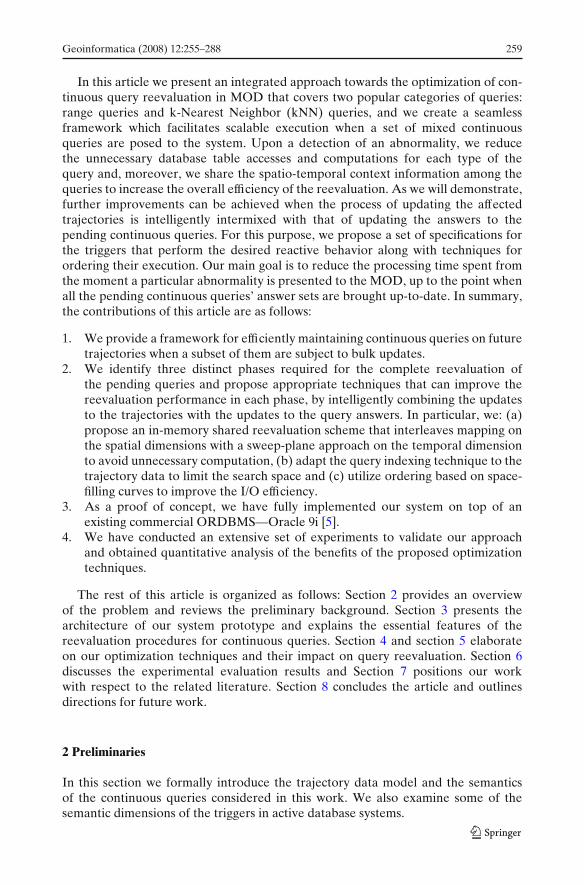
Fig. 6 Space-filling curves

R

a Peano curve (Z-curve)

R

b Hilbert-curve

Note that the queries indexed are a mixture of spatial regions for static rangequeries and querying trajectories for dynamic range queries and kNN queries. Forthe latter two types of queries, when constructing the index, the querying trajectoriesare uniformly split into sub-trajectories using the exact same strategy for splitting thetrajectories in MOT (cf. Section 3).

5.3 Phase 3: Ordering among the triggers

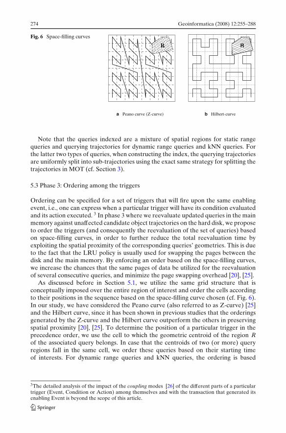
Ordering can be specified for a set of triggers that will fire upon the same enablingevent, i.e., one can express when a particular trigger will have its condition evaluatedand its action executed. 3 In phase 3 where we reevaluate updated queries in the mainmemory against unaffected candidate object trajectories on the hard disk, we proposeto order the triggers (and consequently the reevaluation of the set of queries) basedon space-filling curves, in order to further reduce the total reevaluation time byexploiting the spatial proximity of the corresponding queries’ geometries. This is dueto the fact that the LRU policy is usually used for swapping the pages between thedisk and the main memory. By enforcing an order based on the space-filling curves,we increase the chances that the same pages of data be utilized for the reevaluationof several consecutive queries, and minimize the page swapping overhead [20], [25].

As discussed before in Section 5.1, we utilize the same grid structure that isconceptually imposed over the entire region of interest and order the cells accordingto their positions in the sequence based on the space-filling curve chosen (cf. Fig. 6).In our study, we have considered the Peano curve (also referred to as Z-curve) [25]and the Hilbert curve, since it has been shown in previous studies that the orderingsgenerated by the Z-curve and the Hilbert curve outperform the others in preservingspatial proximity [20], [25]. To determine the position of a particular trigger in theprecedence order, we use the cell to which the geometric centroid of the region Rof the associated query belongs. In case that the centroids of two (or more) queryregions fall in the same cell, we order these queries based on their starting timeof interests. For dynamic range queries and kNN queries, the ordering is based

3The detailed analysis of the impact of the coupling modes [26] of the different parts of a particulartrigger (Event, Condition or Action) among themselves and with the transaction that generated itsenabling Event is beyond the scope of this article.

Geoinformatica (2008) 12:255–288 275

on the individual sub-trajectories, i.e., each sub-trajectory forms a “sub-query” andits reevaluation ordering is determined by the centroid of the MBR of this sub-trajectory. Hence, the reevaluation of a number of queries is actually an intermixedprocess: part of one query is reevaluated followed by the reevaluation of part ofanother query which is spatially close based on the space filling curve.

In order to effectively benefit from the ordering of the triggers’ execution, weenforce an ordering on the candidate objects data as well. The basic idea is toorganize the LOB data for the trajectories in the MOT table according to their spatialproximity. This guarantees that the trajectories that are close to one another will bestored in the same or consecutive disk pages. Hence, portions of different trajectoriesthat are relevant to a particular query will be retrieved with fewer page accesses. Inaddition, as we order the triggers such that consecutive queries will pertain to spatialregions close to each other, pages that were recently read into memory can be fullyutilized before swapped back to disk and thus can further reduce the number of I/Os.

More specifically, when the trajectories of the moving objects are initially bulkloaded into the MOD, they are split into sub-trajectories using the uniform splittingstrategy introduced in Section 3.2. These sub-trajectories are then ordered based thesame space-filling curve used for ordering the queries. We use the centroid of eachsub-trajectory’s 2D projection to decide their relative ordering. Subsequently, thesorted sub-trajectories are stored into MOT in this order. This ensures that the datain the MOT is more or less “spatially clustered” on the hard disk, i.e., a disk page isfilled with sub-trajectories that are spatially close according to the space-filling curve.Note that the ordering of the sub-trajectories takes place during initial bulk loading,and hence it will not incur extra overhead to the reevaluation of the queries.

5.4 Scalable reevaluation for large data sets

The techniques presented in the previous sections utilize the spatio-temporal contextinformation embedded into the trajectories to minimize the unnecessary pairs of(querying trajectory segment, candidate trajectory segment) that are reevaluated,in each of the three phases. However, since the techniques are main memory based,they cannot handle the cases when the data set is too large to fit entirely into themain memory for the reevaluation. This will cause extra data transfer due to pageswapping and can become a source of performance degradation.

Strictly following the phases of Algorithm 1 and converting it into a secondarystorage based algorithm is not a suitable choice. To say the least, this may causesome data items to be purged back to the disk during the reevaluation of a particularphase. However, the same data may be needed from the disk, when executing thenext phase of reevaluation. Aside from the page swapping penalty, the observationthat we just made has another consequence: in effect, we have lost the benefit of theBEFORE option for the semantic dimension of the triggers.

To address this issue, we adapt the divide-and-conquer paradigm and partition theentire MOD data into smaller portions where each one of them alone can be handledusing Algorithm 1. In our system, this is achieved via table partitioning [2]. Morespecifically, we utilize a priori knowledge about the distribution of the trajectorydata, which we collected by performing a preprocessing step that samples over thelarge data set, to determine the number of partitions along each spatial dimension.We ensure that the trajectory data contained in each resulting spatial partition can be

276 Geoinformatica (2008) 12:255–288

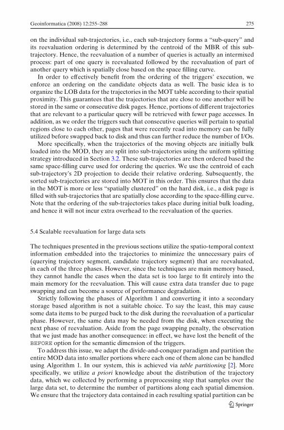
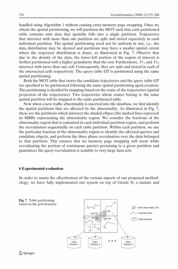
handled using Algorithm 1 without causing extra memory page swapping. Once weobtain the spatial partitioning, we will partition the MOT such that each partitionedtable contains only data that spatially falls into a single partition. Trajectoriesthat intersect with more than one partition are split and stored separately in eachindividual partition. The spatial partitioning need not be uniform in size, i.e., thedata distribution may be skewed and partitions may have a smaller spatial extentwhere the trajectory distribution is dense, as illustrated in Fig. 7. Observe thatdue to the density of the data, the lower-left portion of the region of interest isfurther partitioned with a higher granularity than the rest. Furthermore, Tr1 and Tr2

intersect with more than one cell. Consequently, they are split and stored in each ofthe intersected cells respectively. The query table QT is partitioned using the samespatial partitioning.

Both the MOT table that stores the candidate trajectories and the query table QTare specified to be partitioned following the same spatial partitioning upon creation.The partitioning is decided by mapping based on the route of the trajectories (spatialprojection of the trajectories). Two trajectories whose routes belong to the samespatial partition will be mapped to the same partitioned table.

Now when a new traffic abnormality is inserted into the database, we first identifythe spatial partitions that are affected by the abnormality. As illustrated in Fig. 7,these are the partitions which intersect the shaded ellipse (the dashed lines representits MBR) representing the abnormality region. We consider the fractions of theabnormality region that is contained in each individual partition region, and performthe reevaluation sequentially on each table partition. Within each partition, we usethe particular fraction of the abnormality region to identify the affected queries andcandidate objects, and perform the three phase reevaluation over the data belongedto that partition. This ensures that no memory page swapping will occur whilereevaluating the portion of continuous queries pertaining to a given partition andguarantees the query reevaluation is scalable to very large data sets.

6 Experimental evaluation

In order to assess the effectiveness of the various aspects of our proposed method-ology, we have fully implemented our system on top of Oracle 9i, a mature and

Fig. 7 Table partitioningbased on the grid structure

Table Partition 2

Table Partition 3

Table Partition 1

Traffic Abnormality (TA)

sub-TA1

sub-TA2

sub-TA3 sub-TA4

Trajectory Data

Tr1

Tr2

Table partitions

Trk

Tr3

Tri

Trj

Tr4

Tr5

Geoinformatica (2008) 12:255–288 277

commercially available ORDBMS which, among the others, offers the followingfeatures:

– Triggers, the mechanism which enables declarative specification of reactivebehavior in ORDBMS for the maintenance of continuous queries and part ofthe SQL99 standard [2].

– PL/SQL, a programming language that enables the specification of the pro-cedural aspects of the applications. Our query evaluation and reevaluationalgorithms have been completely implemented using PL/SQL.

– Oracle Spatial [33], which defines what is essentially an abstract data type thatconforms to the object-relational model and is used for modelling various spatialobjects in the database. In our system, we have utilized and extended thedata type to model and represent spatial-temporal trajectories and continuousqueries. More details about our implementation can be found in [6], [11].

6.1 Experimental setup

The experiments were performed on a PC with an Intel Pentium IV CPU 3.6 GHzprocessor, 1 GB of DDR2 memory, an 80 GB SATA hard disk, and with WindowsXP Professional installed. The ORDBMS system that we used is Oracle Release 2,version 9.2.0.1.0.

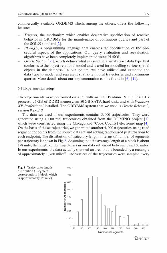
The data set used in our experiments contains 5, 000 trajectories. They weregenerated using 1, 000 real trajectories obtained from the DOMINO project [1],which were constructed using the Chicagoland (Cook County) electronic map [4].On the basis of these trajectories, we generated another 4, 000 trajectories, using roadsegment endpoints from the source data set and adding randomized perturbations toeach endpoint. The distribution of trajectory length in terms of number of segmentsper trajectory is shown in Fig. 8. Assuming that the average length of a block is about1/8 mile, the length of the trajectories in our data set varied between 1 and 60 miles.In our experiments, the data actually spanned an area that is bounded by a rectangleof approximately 1, 780 miles2. The vertices of the trajectories were sampled every

Fig. 8 Trajectories lengthdistribution (1 segmentcorresponds to 1 block, whichis approximately 1/8 mile)

0

100

200

300

400

500

600

700

800

20 60 100 140 180 220 260 300 340 380

Number of Segments

Num

ber

of A

ppea

ranc

es

278 Geoinformatica (2008) 12:255–288

minute, and the duration of the trajectories varied between 20 and 400 min. In ourexperiments, we transform the time measure into discrete units, where 10 time unitscorrespond to 1 min. Thus, the lifetime of MOD is 4, 000 time units.

For static range queries, the query regions were randomly generated within thearea of interest to the MOD, and the time interval spans were distributed evenlythroughout the lifetime of MOD. For dynamic range queries and kNN queries, thequerying trajectories were randomly selected from the 5, 000 trajectories in the dataset, and the radius of the circles for the range queries varied from 1.0 to 5.0 miles.Traffic abnormalities had a duration of 200 time units and could cause the trafficdelay by up to 50% of the normal speed.

The metric that we used in the experimental evaluation is the response time forreevaluating a set of pending continuous queries. We defined the response time to bethe duration from the time instance at which an INSERT request is specified to theTAT table (reflecting a traffic abnormality), until the answer set (Current_Answerattribute in the query table) of every pending query in the MOD is brought up-to-date. The performance is measured using Oracle’s DBMS_PROFILER package.

6.2 Experimental results

First we demonstrate the effectiveness of each of our context-aware optimizationtechniques in isolation. We then present a combined approach to compare theoverall performance of our optimized query reevaluation approach against a naiveapproach, which works in a brute force manner without utilizing any of our proposedtechniques.

6.2.1 Semantic dimensions of the triggers

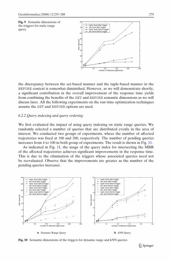
When it comes to the different semantic dimensions used in the specification of aparticular trigger, we investigated two of them: (1) BEFORE vs. AFTER execution,which specifies the mode in which the modifications to the database are appliedwith respect to the action part of the trigger; (2) SET vs. TUPLE execution, whichspecifies the level of granularity of applying the modifications to the database andits relationship with the trigger. Combining each of the values, we have four possibleoptions and we measured the running times for each of them. In the experiments, wefocused on one single query (consequently, one trigger) and we varied the numberof trajectories affected by the traffic abnormality from 8 to 200, by changing thespatial location and time interval of the disturbance zone. For a static range query,the average response times are shown in Fig. 9. The cases for the dynamic rangequeries and kNN queries are shown in Fig. 10a and b, respectively. The dotted linesrepresent the case when the querying trajectory is not affected by the abnormality,where only the second phase of reevaluation need to be executed. The solid linesrepresent the case when the query trajectory is also affected by the abnormalityand need to be updated, and all three phases of reevaluation are necessary. Allthree groups of experiments have provided consistent outcomes. As expected, thebest performance is obtained when the BEFORE trigger executes in a SET orientedmanner, improving the response time by up to 85% compared with the worst caserunning time. A noteworthy observation is that loading the Oracle Spatial packageincurs a substantial context-switching time penalty and this is part of the reason why

Geoinformatica (2008) 12:255–288 279

Fig. 9 Semantic dimensions ofthe triggers for static rangequery

0 50 100 150 200 2500

10

20

30

40

50

60

70

80

number of affected trajectories

time

(sec

ond)

tuple–level after triggerset–level after triggertuple–level before triggerset–level before trigger

the discrepancy between the set-based manner and the tuple-based manner in theBEFORE context is somewhat diminished. However, as we will demonstrate shortly,a significant contribution in the overall improvement of the response time yieldsfrom combining the benefits of the SET and BEFORE semantic dimensions as we willdiscuss later. All the following experiments on the run-time optimization techniquesassume the SET and BEFORE options are used.

6.2.2 Query indexing and query ordering

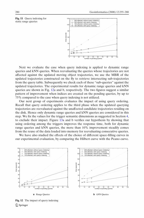
We first evaluated the impact of using query indexing on static range queries. Werandomly selected a number of queries that are distributed evenly in the area ofinterest. We conducted two groups of experiments, where the number of affectedtrajectories was fixed at 100 and 200, respectively. The number of pending queriesincreases from 4 to 100 in both group of experiments. The result is shown in Fig. 11.

As indicated in Fig. 11, the usage of the query index for intersecting the MBRof the affected trajectories achieves significant improvements in the response time.This is due to the elimination of the triggers whose associated queries need notbe reevaluated. Observe that the improvements are greater as the number of thepending queries increases.

0 50 100 150 200 2500

20

40

60

80

100

120

140

number of affected trajectories

time

(sec

ond)

tuple–level after triggerset–level after triggertuple–level before triggerset–level before triggertuple–level after triggerset–level after triggertuple–level before triggerset–level before trigger

a Dynamic Range Query

0 50 100 150 200 2500

20

40

60

80

100

120

number of affected trajectories

time

(sec

ond)

tuple–level after triggerset–level after triggertuple–level before triggerset–level before triggertuple–level after triggerset–level after triggertuple–level before triggerset–level before trigger

b kNN Query

Fig. 10 Semantic dimensions of the triggers for dynamic range and kNN queries

280 Geoinformatica (2008) 12:255–288

Fig. 11 Query indexing forstatic range queries

0 10 20 30 40 50 60 70 80 90 1000

20

40

60

80

100

120

number of pending queries

time

(sec

ond)

200 affected, without query–indexing200 affected, with query–indexing100 affected, without query–indexing100 affected, with query–indexing

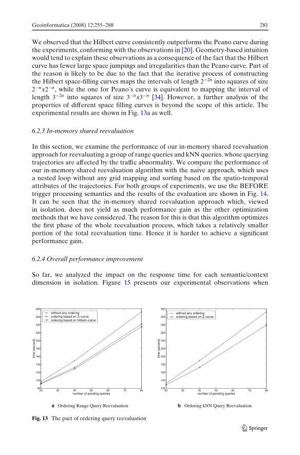
Next we evaluate the case when query indexing is applied to dynamic rangequeries and kNN queries. When reevaluating the queries whose trajectories are notaffected against the updated moving object trajectories, we use the MBR of theupdated trajectories constructed on the fly to retrieve intersecting sub-trajectoriesfrom the query table. Subsequently we check each of these “sub-queries” against theupdated trajectories. The experimental results for dynamic range queries and kNNqueries are shown in Fig. 12a and b, respectively. The two figures suggest a similarpattern of improvement when indices are created on the pending queries, by up to75% compared to the case when query indexing is not utilized.

Our next group of experiments evaluates the impact of using query ordering.Recall that query ordering applies to the third phase when the updated queryingtrajectories are reevaluated against the unaffected candidate trajectories residing onthe disk. Hence only dynamic range queries and kNN queries are considered in thisstep. We fix the values for the trigger semantic dimensions as suggested in Section 4,to exclude their impact. Figure 13a and b verifies our hypothesis by showing thatusing ordering among the triggers improves the response time, both for dynamicrange queries and kNN queries, the more than 10% improvement steadily comesfrom the reuse of the data loaded into memory for reevaluating consecutive queries.

We have also studied the effects of the choice of different space-filling curves inour experimental evaluation, by comparing the Hilbert curve with the Peano curve.

0 10 20 30 40 50 60 70 80 90 1000

10

20

30

40

50

60

70

80

90

100

number of pending queries

time

(sec

ond)

200 affected, without query–indexing200 affected, with query–indexing100 affected, without query–indexing100 affected, with queryi–ndexing

a Range Queries

0 10 20 30 40 50 60 70 80 90 1000

20

40

60

80

100

120

140

number of pending queries

time

(sec

ond)

200 affected, without query–indexing200 affected, with query–indexing100 affected, without query–indexing100 affected, with query–indexing

b kNN Queries

Fig. 12 The impact of query indexing

Geoinformatica (2008) 12:255–288 281

We observed that the Hilbert curve consistently outperforms the Peano curve duringthe experiments, conforming with the observations in [20]. Geometry-based intuitionwould tend to explain these observations as a consequence of the fact that the Hilbertcurve has fewer large space jumpings and irregularities than the Peano curve. Part ofthe reason is likely to be due to the fact that the iterative process of constructingthe Hilbert space-filling curves maps the intervals of length 2−2n into squares of size2−nx2−n, while the one for Peano’s curve is equivalent to mapping the interval oflength 3−2n into squares of size 3−nx3−n [34]. However, a further analysis of theproperties of different space filling curves is beyond the scope of this article. Theexperimental results are shown in Fig. 13a as well.

6.2.3 In-memory shared reevaluation

In this section, we examine the performance of our in-memory shared reevaluationapproach for reevaluating a group of range queries and kNN queries, whose queryingtrajectories are affected by the traffic abnormality. We compare the performance ofour in-memory shared reevaluation algorithm with the naive approach, which usesa nested loop without any grid mapping and sorting based on the spatio-temporalattributes of the trajectories. For both groups of experiments, we use the BEFOREtrigger processing semantics and the results of the evaluation are shown in Fig. 14.It can be seen that the in-memory shared reevaluation approach which, viewedin isolation, does not yield as much performance gain as the other optimizationmethods that we have considered. The reason for this is that this algorithm optimizesthe first phase of the whole reevaluation process, which takes a relatively smallerportion of the total reevaluation time. Hence it is harder to achieve a significantperformance gain.

6.2.4 Overall performance improvement

So far, we analyzed the impact on the response time for each semantic/contextdimension in isolation. Figure 15 presents our experimental observations when

20 30 40 50 60 70 8080

100

120

140

160

180

200

220

240

260

280

number of pending queries

time

(sec

ond)

without any orderingordering based on Z–curveordering based on Hilbert–curve

a Ordering Range Query Reevaluation

20 30 40 50 60 70 80120

140

160

180

200

220

240

260

280

300

320

number of pending queries

time

(sec

ond)

without any orderingordering based on Z–curve

b Ordering kNN Query Reevaluation

Fig. 13 The pact of ordering query reevaluation

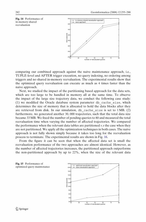
282 Geoinformatica (2008) 12:255–288

Fig. 14 Performance ofin-memory sharedreevaluation

20 30 40 50 60 70 80200

250

300

350

400

450

500

550

number of reevaluated queries

time

(sec

ond)

in–memory shared reevaluation approachnaive approach

comparing our combined approach against the naive maintenance approach, i.e.,TUPLE-level and AFTER trigger execution, no query indexing, no ordering amongtriggers and no shared in-memory reevaluation. The experimental results show thatthe optimized query reevaluation can execute as much as 4 times faster than thenaive approach.

Next, we studied the impact of the partitioning based approach for the data sets,which are too large to be handled in memory all at the same time. To observethe impact of the large size trajectory data, we conduct the following case study:(1) we modified the Oracle database system parameter db_cache_size, whichdetermines the size of memory that is allocated to hold the data blocks after theyare retrieved from disk. In our simulation, db_cache_size is set to 1 MB. (2)furthermore, we generated another 30, 000 trajectories, such that the total data sizebecame 33 MB. We fixed the number of pending queries to 80 and measured the totalreevaluation time when varying the number of affected trajectories. We comparedthe performance when the relevant data tables are partitioned v.s the case when theyare not partitioned. We apply all the optimization techniques in both cases. The naiveapproach is not fully shown simply because it takes too long for the reevaluationprocess to terminate. The experimental results are shown in Fig. 16.

From the figure it can be seen that when the affected data set is small thereevaluation performance of the two approaches are almost identical. However, asthe number of affected trajectories increases, the partitioned approach outperformsthe non-partitioned approach by up to 22%, when the size of the relevant data

Fig. 15 Performance ofoptimized query maintenance

20 30 40 50 60 70 80200

400

600

800

1000

1200

1400

1600

1800

2000

2200

number of reevaluated queries

time

(sec

ond)

optimized reevaluation approachnaive reevaluation approach

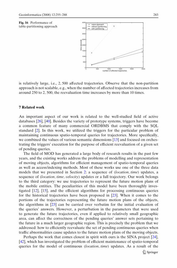
Geoinformatica (2008) 12:255–288 283

Fig. 16 Performance oftable-partitioning approach

0 500 1000 1500 2000 25000

500

1000

1500

2000

2500

3000

3500

4000

number of affected trajectories

time

(sec

ond)

naive approachwithout partitioningwith partitioning

is relatively large, i.e., 2, 500 affected trajectories. Observe that the non-partitionapproach is not scalable, e.g., when the number of affected trajectories increases fromaround 250 to 2, 500, the reevaluation time increases by more than 10 times.

7 Related work

An important aspect of our work is related to the well-studied field of activedatabases [26], [40]. Besides the variety of prototype systems, triggers have becomea common feature of many commercial ORDBMS that comply with the SQLstandard [2]. In this work, we utilized the triggers for the particular problem ofmaintaining continuous spatio-temporal queries for trajectories. More specifically,we combined the values of various semantic dimensions [13] and focused on orches-trating the triggers’ execution for the purpose of efficient reevaluation of a given setof pending queries.

The field of MOD has generated a large body of research results in the past fewyears, and the existing works address the problems of modelling and representationof moving objects, algorithms for efficient management of spatio-temporal queriesas well as access/indexing methods. Most of these works use one of the three datamodels that we presented in Section 2: a sequence of (location, time) updates, asequence of (location, time, velocity) updates or a full trajectory. Our work belongsto the third category: we use trajectories to represent the future motion plans ofthe mobile entities. The peculiarities of this model have been thoroughly inves-tigated [12], [15], and the efficient algorithms for processing continuous queriesfor the historical trajectories have been proposed in [23]. When it comes to theportions of the trajectories representing the future motion plans of the objects,the algorithms in [23] can be carried over verbatim for the initial evaluation ofthe queries’ answers. However, a perturbation in the parameters that were usedto generate the future trajectories, even if applied to relatively small geographicarea, can affect the correctness of the pending queries’ answer sets pertaining tothe future in a much larger geographic region. This is precisely the problem that weaddressed: how to efficiently reevaluate the set of pending continuous queries whentraffic abnormalities cause updates to the future motion plans of the moving objects.

Perhaps the work that comes closest in spirit with ours is the SINA project [24],[42], which has investigated the problem of efficient maintenance of spatio-temporalqueries for the model of continuous (location, time) updates. As a result of the

284 Geoinformatica (2008) 12:255–288

different models, the underlying algorithms for maintaining the continuous queriesare different. In SINA, query maintenance has to be performed periodically at a highfrequency, whenever updates are available. Furthermore, the query maintenanceexhibits some spatial locality because a subsequent update is in general close tothe previous one, while in our case a local update may impact queries that spanover a much larger geographic regions. Its recent extensions have also consideredthe lazy buffering approach for balancing the trade-offs between data updates andquery reevaluation [43]. If the adopted model is the (location, time, velocity) updatesto the MOD [35], the system can afford to “see” a bit further into the future andavoid constant reevaluation of the pending queries. However, when updates arrive,a larger set of spatio-temporally correlated queries may need to be reevaluated in abulk manner [19]. In this sense, our work covers the “far-end of the spectrum”: withthe trajectories pertaining to the future motions of the moving objects, one can poseand obtain the answer sets to the various continuous queries pertaining to any futuretime interval. However, the main penalty is the reevaluation due to the impact ofsome potential traffic abnormality that may affect a large number of queries whichneed not be in a close geographic proximity.

Investigation into the essential properties of efficient indexing structures in spatio-temporal settings were presented by Theodoridis et al. [37]. It has also been observedthat straightforwardly using an R-tree [17] or its variants, e.g., the R∗ tree [7] onspatio-temporal trajectory data will introduce a large amount of dead space. Severalindexing methods have been proposed that try to reduce the impact of the dead spacefor trajectories. For example, Pfoser et al. [28] attempt to preserve the segments thatbelong to the same trajectory, and the problem of obtaining an efficient splitting ofthe trajectory segments has been further investigated in [8], [18], [32]. In our work,we relied on the R∗ tree indexing mechanism that is readily available in Oracle9i [33], for indexing the two dimensional routes of the trajectories. However, wehave adopted it for various needs, e.g., indexing the trajectory segments, using thetime information of trajectories in a refinement step etc.

The idea of indexing the queries instead of moving objects, for the purpose ofefficient spatio-temporal query processing was presented in [31], and was furtherextended for in-memory evaluation in [21]. However, the motion model used there—a sequence of (location, time) updates as the objects are moving—is different fromour data model of the trajectories. This in turn requires a different reactive behaviorand consequently processing algorithms. The utilization of space-filling curves toimpose a linear order on the spatial-temporal objects has been investigated by Jensenet al. [20], which reports access efficiency obtained from the linear ordering. On theother hand, we adopted the space-filling curves for sequencing the reevaluation ofthe pending queries, in order to reduce the context switching costs among differentqueries.

8 Conclusions and future work

The efficient maintenance of continuous queries over moving objects is essentialwhen providing location-based services. In this article, we addressed the issues thatarise when reevaluating a set of continuous queries over the trajectories that are usedto model the future motion plans of the moving objects, which is an extension of

Geoinformatica (2008) 12:255–288 285

our earlier framework [38]. Towards this, we proposed a context-aware approach foroptimization and identified opportunities for performance tuning at various levels.We proposed several context-aware optimization techniques that can substantiallyreduce the query reevaluation time, and analyzed the impact that each of them hason various continuous queries, e.g., range queries and kNN queries.

Our query reevaluation begins by setting up relevant triggers that watch themoving objects table and the pending queries table, as new traffic abnormalities arereported. We identified at least three major sources of context-switching overheadand unnecessary disk I/Os incurred at the operating system level, if the triggers arenot specified properly. We analyzed the trigger execution process and found that theoptimal performance is expected when the triggers are specified to execute at theSET level, and in the BEFORE manner.

The first step in the query reevaluation is to retrieve the affected queryingtrajectories and candidate trajectories into main memory, and update them to reflectthe impact of the traffic abnormality. The unaffected queries and candidate objectsremain on the disk. Then, the query reevaluation takes three phases to complete:

– In the first phase, the affected queries are reevaluated against the affected can-didate trajectories. We employed an in-memory shared reevaluation algorithmto utilize the spatio-temporal information embedded in the data and effectivelyreduce the amount of computation for reevaluating querying trajectory segmentsagainst candidate trajectory segments.

– In the second phase, the affected candidate trajectories are checked against theunaffected queries on disk. We utilized an R-tree index built on the queriesto reevaluate only the set of relevant queries and thus improve reevaluationefficiency by limiting the search space.

– In the third phase, the affected queries are reevaluated against the unaffectedcandidate trajectories on disk. We ordered the queries to be reevaluated as wellas the on-disk data (the segments of trajectories) based on a space-filling curve topreserve spatial proximity. This reduces the number of disk pages to be retrievedand avoids potential memory page swapping.

We also considered the case where the entire set of affected data cannot beaccommodated in the main memory at the same time. We proposed to partition therelevant data tables according to a grid structure, such that each partition can fit intothe memory in order to avoid unnecessary memory page swapping. The reevaluationcycles over all the partitions affected by the traffic abnormality executing each of thethree phases.

We have built our system prototype on top of an industry-strength ORDBMS—Oracle 9i, making maximum use of the existing commercial database capability.We have conducted extensive experiments to observe the benefits of our proposedtechniques. We would like to point out that our approach is not strictly limited toOracle 9i. In fact, any ORDBMS that conforms to the SQL-99 standard [2] andsupports specifying User-Defined Types (UDT) and implementing User-DefinedFunctions (UDF) can be used as a foundation of our implementation.

There are a few potential opportunities for future research work. Currently we areworking on incorporate uncertainty into the query maintenance process, i.e., a userwho posed a continuous query may receive answers that come with a probabilistic

286 Geoinformatica (2008) 12:255–288

attribute, which more realistically reflects the status of moving objects [29]. We arealso working on incorporating some other optimization techniques such as sharedmemory buffer and data prefetching to improve the execution of the set of enabledtriggers in the ORDBMS. Another interesting problem is how to utilize in ourapproach information of the underlying road networks [27] to further improve theefficiency of the reevaluation procedure.

References

1. DOMINO project at DBMC laboratory, UIC. http://www.cs.uic.edu/∼wolfson/html/mobile.html.2. ANSI/ISO international standard: Database language SQL. http://webstore.ansi.org.3. Forbes online issue, April 13, 2006. http://www.forbes.com/home/digitalentertainment/2006/04/13/

google-aol-yahoo -cx_rr_0417maps.html.4. Geographic Data Technology. http://www.geographic.com.5. Oracle 9i. http://www.oracle.com/technology/products/oracle9i.6. H. Ding. Context Aware Optimization of Continuous Query Maintenance for Trajectories. M.S.

thesis, Dept. of EECS, Northwestern University, 2005.7. N. Beckmann, H.-P. Kriegel, R. Schneider, and B. Seeger. “ The R*-Tree: An efficient and robust

access method for points and rectangles,” in Proc. of SIGMOD Conference, pp. 322–331, 1990.8. V.P. Chakka, A. Everspaugh, and J.M. Patel. “Indexing large trajectory data sets with SETI,” in

Proc. of CIDR, 2003.9. E.W. Cheney and D.R. Kincaid. Numerical Mathematics and Computing. Brooks Cole, 2003.

10. T.H. Cormen, C.E. Leiserson, and R.L. Rivest. Introduction to Algorithms. McGraw-Hill, NY,1990.

11. H. Ding, G. Trajcevski, and P. Scheuermann. “Omcat: optimal maintenance of continuousqueries’ answers for trajectories,” in Proc. of SIGMOD Conference, pp. 748–750, 2006.

12. L. Forlizzi, R.H. Güting, E. Nardelli, and M. Schneider. “ A data model and data structures formoving objects databases,” in Proc. of SIGMOD Conference, pp. 319–330, 2000.

13. P. Fraternali and L. Tanca. “ A structured approach for the definition of the semantics of activedatabases,” ACM Transactions on Database Systems, Vol. 20(4):414–471, 1995.

14. B. Gedik and L. Liu. “Mobieyes: Distributed processing of continuously moving queries onmoving objects in a mobile system,” in Proc. of EDBT, pp. 67–87, 2004.

15. R.H. Güting, M.H. Böhlen, M. Erwig, C.S. Jensen, N.A. Lorentzos, M. Schneider, andM. Vazirgiannis. “A foundation for representing and querying moving objects,” ACM Trans-actions on Database Systems, Vol. 25(1):1.

16. R.H. Güting and M. Schneider. Moving Object Databases. Morgan Kaufmann, CA, 2005.17. A. Guttman. “R-trees: A dynamic index structure for spatial searching,” in B. Yormark

(Ed.), SIGMOD’84, Proceedings of Annual Meeting, Boston, Massachusetts, June 18–21, 1984,pp. 47–57. ACM Press, 1984.

18. M. Hadjieleftheriou, G. Kollios, V.J. Tsotras, and D. Gunopulos. “Efficient indexing of spa-tiotemporal objects,” in Proc. of EDBT, pp. 251–268, 2002.

19. G.S. Iwerks, H. Samet, and K.Smith. “Continuous k-nearest neighbor queries for continuouslymoving points with updates,” in Proc. of VLDB, pp. 512–523, 2003.

20. C.S. Jensen, D. Lin, and B.C. Ooi. “Query and update efficient b+-tree based indexing of movingobjects,” in Proc. of VLDB, pp. 768–779, 2004.

21. D.V. Kalashnikov, S. Prabhakar, S.E. Hambrusch, and W.G. Aref. “Efficient evaluation ofcontinuous range queries on moving objects,” in DEXA, pp. 731–740, 2002.

22. M. Koubarakis, T.K. Sellis, A.U. Frank, S. Grumbach, R.H. Güting, C.S. Jensen, N.A.Lorentzos, Y. Manolopoulos, E. Nardelli, B. Pernici, H.-J. Schek, M. Scholl, B. Theodoulidis,and N. Tryfona, (Eds.), Spatio-Temporal Databases: The CHOROCHRONOS Approach,volume 2520 of Lecture Notes in Computer Science. Springer, 2003.

23. J.A.C. Lema, L. Forlizzi, R.H. Güting, E. Nardelli, and M. Schneider. “Algorithms for movingobjects databases,” Computer Journalen, Vol. 46(6):680–712, 2003.

24. M.F. Mokbel, X. Xiong, and W.G. Aref. SINA: Scalable incremental processing of contin-uous queries in spatio-temporal databases. in Proc. of SIGMOD Conference, pp. 623–634,2004.

Geoinformatica (2008) 12:255–288 287

25. B. Moon, H.V. Jagadish, C. Faloutsos, and J.H. Saltz. “Analysis of the clustering properties ofthe hilbert space-filling curve,” IEEE Transactions on Knowledge and Data Engineering, Vol.13(1):124–141, 2001.

26. N.W. Paton (Ed.), Active Rules in Database Systems. Springer, New York, 1999.27. D. Pfoser and C.S. Jensen. “Trajectory indexing using movement constraints*,” GeoInformatica,

Vol. 9(2):93–115, 2005.28. D. Pfoser, C.S. Jensen, and Y. Theodoridis. “Novel approaches in query processing for moving

object trajectories,” in Proc. of VLDB, pp. 395–406, 2000.29. D. Pfoser, N. Tryfona, and C.S. Jensen. “Indeterminacy and spatiotemporal data: Basic defini-

tions and case study,” GeoInformatica, Vol. 9(3):211–236, 2005.30. E. Pitoura and G. Samaras. Locating objects in mobile computing. IEEE Transactions on Knowl-

edge and Data Engineering, Vol. 13(4):571–592, 2001.31. S. Prabhakar, Y. Xia, D.V. Kalashnikov, W.G. Aref, and S.E. Hambrusch. “Query index-

ing and velocity constrained indexing: Scalable techniques for continuous queries on movingobjects,” IEEE Transactions on Computers, Vol. 51(10):1124–1140, 2002.

32. S. Rasetic, J. Sander, J. Elding, and M.A. Nascimento. “A trajectory splitting model for efficientspatio-temporal indexing,” in Proc. of VLDB, pp. 934–945, 2005.

33. R. Kothuri, A. Godfrind and E. Beinat. Pro Oracle Spatial. Apress, 2004.34. H. Sagan. Space-filling Curves. Springer, 1994.35. A.P. Sistla, O. Wolfson, S. Chamberlain, and S. Dao. “Modeling and querying moving objects,”

in Proc. of ICDE, pp. 422–432, 1997.36. Y. Tao and D. Papadias. “Time-parameterized queries in spatio-temporal databases,” in Proc. of

SIGMOD Conference, pp. 334–345, 2002.37. Y. Theodoridis, T.K. Sellis, A. Papadopoulos, and Y. Manolopoulos. “Specifications for efficient

indexing in spatiotemporal databases,” in Proc. of SSDBM, pp. 123–132, 1998.38. G. Trajcevski, H.Ding, and P. Scheuermann. “Context-aware optimization of continuous range

queries maintenance for trajectories,” in MobiDE, pp. 1–8, 2005.39. G. Trajcevski, O. Wolfson, K. Hinrichs, and S. Chamberlain. “Managing uncertainty in moving

objects databases,” ACM Trans. Database Syst., Vol. 29(3):463–507, 2004.40. J. Widom and S. Ceri. Active Database Systems. 1995.41. O. Wolfson, A.P. Sistla, S. Chamberlain, and Y. Yesha. “Updating and querying databases that

track mobile units,” Distributed and Parallel Databases, Vol. 7(3):257–387, 1999.42. X. Xiong, M.F. Mokbel, W.G. Aref, S.E. Hambrusch, and S. Prabhakar. “Scalable spatio-

temporal continuous query processing for location-aware services,” in Proc. of SSDBM, p. 317,2004.

43. X. Xiong and W.G. Aref. “R-trees with update memos” in Proc. of ICDE, 2006.

Hui Ding received the B.E. degree in electronic engineering from Tsinghua University, Beijing,China in 2003. He is now a Ph.D. student in the deparment of electrical engineering and computerscience at Northwestern University, U.S.A. His research interest is in spatio-temporal databases anddata management in mobile computing.

288 Geoinformatica (2008) 12:255–288

Goce Trajcevski is a researcher at the Dept. of Electrical Engineering and Computer Science atthe Northwestern University. His main interests are in the areas of mobile data management andsensor networks. He received a BS from the University of Sts. Kiril & Metodi, and the MS and PhDfrom the University of Illinois at Chicago. He coauthored over 25 publications, participated as aPC member of several conferences and workshops, and was ACM DiSC associate editor 2003–2005.He is a member of IEEE and ACM.

Peter Scheuermann is a Professor of Electrical Engineering and Computer Science at NorthwesternUniversity. He has held visiting professor positions with the Free University of Amsterdam, theUniversity of Hamburg and the Swiss Federal Institute of Technology, Zurich. During 1997–1998he served as Program Director for Operating Systems at the NSF. Dr. Scheuermann has servedon the editorial board of the Communications of ACM, The VLB Journal and IEEE Transactionson Knowledge and Data Engineering. His current research interests are in parallel and distributeddatabase systems, mobile computing, spatial databases and data mining. He has published more than100 journal and conference papers. Peter Scheuermann is a Fellow of IEEE.