This is a preprint of an article accepted for publication in Journal of Applied

Mathematical Modelling on 29 April 2014. The published article is available online at

http://www.sciencedirect.com/science/article/pii/S0307904X14002418

To be cited as: Bouaanani N., Miquel B. 2015. Efficient modal dynamic analysis of flexible beam-fluid

systems. Journal of Applied Mathematical Modelling, 1: 99–116.

Efficient Modal Dynamic Analysisof Flexible Beam-Fluid Systems

Najib Bouaanani1 and Benjamin Miquel2

ABSTRACT

This paper proposes an efficient simplified method to determine the modal dynamic and earthquake re-

sponse of coupled flexible beam-fluid systems and to evaluatetheir natural vibration frequencies. The

methodology developed extends available analytical solutions for mode shapes and natural vibration

frequencies of slender beams with various boundary conditions to include the effects of fluid-structure

interaction. The proposed method is developed for various beam boundary conditions considering

lateral interaction with one or two semi-infinite fluid domains. Numerical examples are provided to

illustrate the application of the proposed method, and the obtained results confirm the importance of

accounting for fluid-structure interaction effects. We show that the developed procedure yields excel-

lent results when compared to more advanced coupled fluid-structure finite element solutions, inde-

pendently of the number of included modes, beam boundary conditions, and number of interacting

fluid domains. The proposed simplified method can be easily implemented in day-to-day engineer-

ing practice, as it constitutes an efficient alternative solution considering the fluid-structure modeling

complexities and related high expertise generally involved when using advanced finite elements.

Key words: Dynamic and seismic effects; Beam-fluid systems; Natural frequencies; Simplified

methods; Fluid-Structure interaction; Finite elements.

1 Professor, Department of Civil, Geological and Mining Engineering,Polytechnique Montréal, Montréal, QC H3C 3A7, Canada.Corresponding author. E-mail: najib.bouaanani@polymtl.ca2 Graduate Research Assistant, Department of Civil, Geological and Mining Engineering,Polytechnique Montréal, Montréal, QC H3C 3A7, Canada.

1 Introduction

Several civil engineering and industrial applications involve the vibrations of beam-like struc-

tures in contact with water or fluid domains, including dams,navigation locks, quay walls,

break-waters, offshore platforms, drilling risers, liquid storages, nuclear reactors, oil refiner-

ies, petrochemical plants, fuel storage racks, etc. This popular topic has attracted many re-

searchers over the last decades and various approaches wereproposed, varying from simpli-

fied to more complex analytical and numerical formulations.Neglecting structural flexibility,

Westergaard [1] introduced the added-mass concept and applied it to a dam-reservoir system,

and later Jacobsen [2] and Rao [3] generalized the added-mass formulation to evaluate hydro-

dynamic effects on rigid circular and rectangular piers vibrating in water. Goto and Toki [4]

and Kotsubo [5] evaluated the hydrodynamic pressures induced by harmonic motions on

circular or elliptical cross-section cylindrical towers along rigid body and deformed mode

shapes. Chopra [6, 7] showed that a dam’s flexibility influences significantly its interaction

with the impounded reservoir, and consequently the overalldynamic and seismic responses.

Other studies also confirmed the importance of accounting for structural flexibility and fluid-

structure interaction [8–11]. Han and Xu [12] developed an analytical model to compute the

modal properties of a slender flexible cylinder vibrating inwater, and proposed a simplified

added-mass formula to compute its natural frequencies. Other researchers studied the sensi-

tivity of the hydrodynamic response of cantilever structures to various factors, such as: (i) a

tip mass or inertia concentrated at one end [13–16], (ii) a restrained boundary condition at

the base of the beam [16–18], and (iii) non-uniformity of beam cross-section [16,17,19].

Most of the previous studies focused on cantilever structures surrounded by fluid. Work on

beam-like structures interacting with 2D semi-infinite fluid domains was mainly related to

dam monoliths impounding water reservoirs, while fewer researchers investigated the behav-

ior of slender beams subjected to hydrodynamic loading of the latter type. Xing et al. [20],

Zhao et al. [21] and Xing [22] developed analytical formulations to examine the dynamic

response of a cantilever flexible beam interacting with a 2D semi-infinite water domain, and

discussed the effects of various boundary conditions of thefluid domain. Nasserzare et al. [23]

proposed a procedure to extract the natural frequencies andmodes of a dry structure from vi-

brational data containing fluid-structure interaction effects, and they applied the methodology

to a beam-water system. De Souza and Pedroso [24] developed afinite element procedure to

determine the coupled dynamic response of a Bernoulli beam interacting with a 2D acousti-

cal cavity, and they validated the vibration frequencies and modes obtained by comparing to

other finite element and analytical solutions.

The present paper is motivated by the need to develop simplified methods extending results

from classical vibration beam theory to include the effectsof 2D hydrodynamic forces on

one or both sides of a vibrating beam. The majority of the previous work and other relevant

literature addressed hydrodynamic effects on cantilever beams, fully clamped or partially

2

restrained at the base, and little attention has been given to other boundary conditions such as

pinned or sliding supports. Most of the previous studies also focused on the determination of

the modal properties of a vibrating beam interacting with a fluid, while less concern has been

devoted to the time evolution of beam’s earthquake responseindexes such as displacements,

shear forces, and bending moments. These restrictions willbe addressed in this paper.

2 Modal dynamic response of a beam-fluid system

2.1 Basic assumptions and notation

Fig. 1 shows a slender beam of heightH vibrating in contact with fluid on one or both sides.

We adopt a Cartesian coordinate system with origin at the base of the beam, a horizontal axis

x and a vertical axisy coincident with the axis of symmetry of the beam. The semi-infinite

fluid domains have a rectangular geometry with constant height equal to that of the beam.

We denote byΛf the number of fluid domains in contact with the beam, and by left and right

side fluid domains those extending from the beam towards negative and positivex directions,

respectively. Both configurations illustrated in Figs. 1 (a) and (b) will be investigated here,

i.e.Λf =1 andΛf =2, respectively. The beam will be referred to as dry when it is in contact

with one fluid domain at least, i.e.Λf > 0, and wet otherwise. The boundary conditions of

the beam can be Clamped-Free (CF) as shown in Fig. 1 or Clamped-Pinned (CP), Clamped-

Sliding (CS), Clamped-Clamped (CC) or Pinned-Pinned (PP) as illustrated in Fig. 2. Points

at the top, middle and base of the beam are denoted by A, B and C,respectively, as shown in

Fig. 1 (a). These points will be used later to illustrate various dynamic responses of the stud-

ied beams. We also assume that: (i) the beam is slender so thatonly flexural deformations

are considered, i.e. Euler-Benoulli beam theory is used; (ii) the beam is made of a linear,

homogenous, and isotropic elastic material; (iii) only small deflections normal to the unde-

formed beam axis are included; (iv) the fluid is incompressible and inviscid, with its motion

irrotational and limited to small amplitudes, (v) the fluid remains in full contact with the beam

during vibration due to the assumption of small displacements, and (vi) gravity surface waves

and non-convective effects are neglected.

2.2 Governing equations

We first assume that the beam-fluid system is subjected to a unit harmonic free-field horizon-

tal ground motionug(t)=eiωt, whereω denotes a forcing frequency,t the time variable and i

the unit imaginary number. Using a modal superposition analysis, the frequency response

functions along beam’s height of lateral displacementu, lateral accelerationu, bending mo-

3

mentM and shear forceV can be expressed as

u(y, ω) =Ns∑

j=1

ψj(y) Zj(ω) ; ¯u(y, ω) = −ω2Ns∑

j=1

ψj(y) Zj(ω) (1)

M(y, ω) = EINs∑

j=1

Zj(ω)∂2ψj(y)

∂y2; V(y, ω) = EI

Ns∑

j=1

Zj(ω)∂3ψj(y)

∂y3(2)

whereNs denotes the number of dry beam modes included in the analysis,ψj thex–component

of thej th vibration mode shapeψj , j=1 . . . Ns, of the dry beam,Zj the corresponding gen-

eralized coordinate,E the modulus of elasticity of the beam andI the moment of inertia of

the beam about bending neutral axis.

Based on previous studies [25–27], the vectorZ of generalized coordinatesZj(ω), j =

1 . . .Ns, can be obtained by solving the system of equations

S Z = Q (3)

which translates the beam-fluid system’s dynamic equilibrium between inertia, damping and

elastic forces resulting from the vibrations of the beam andhydrodynamic forces generated

by the interacting fluid domain(s). The elements of matrixS and vectorQ in Eq. (3) are

obtained forj = 1 . . .Ns andm = 1 . . .Ns as

Sj,m(ω) =[− ω2 + (1 + i η)ω2

j

]Mj δj,m − Λf ω

2∫ H

0pj(y, ω)ψm(y) dy (4)

and

Qm = −Lm − Λf

∫ H

0p0(y, ω)ψm(y) dy (5)

in whichδj,m denotes the Kronecker symbol and

– p0 is the frequency response function for hydrodynamic pressure exerted on the left side of

the beam due to its rigid body motion;

– pj is the frequency response function for hydrodynamic pressure exerted on the left side of

the beam due to its horizontal accelerationψj(y);

– ωj is the natural frequency corresponding to thej th dry beam vibration mode shapeψj ;

– η is an assumed constant hysteretic damping ratio;

– Mj andLm are respectively the generalized mass and force given by

Mj = µs

∫ H

0[ψj(y)]

2 dy = µsH∫ 1

0

[ψj(y)

]2dy = µsHM∗

j (6)

Lm = µs

∫ H

0ψm(y) dy = µsH

∫ 1

0ψm(y) dy = µsH L∗

m (7)

in which µs is the beam’s mass per unit height andψ is a function resulting from the

introduction of the change of variabley=y/H into the mode shape functionψj .

4

The mode shapes for slender beams were reported in many references such as [28–31]. The

formulation given by Young and Felgar [28] and Blevins [30] is adopted here. The expres-

sions of beam mode shapes are reviewed in Appendix A for the studied beam boundary con-

ditions illustrated in Fig. 2. For each beam configuration, the expressions for parametersβjandσj , j = 1 . . .Ns, required to obtain beam mode shapes are provided in Table A1. These

parameters are computed using high precision arithmetic for the first10 beam modes, i.e.

Ns=10, and are given in Tables 1 to 7 for all the beam configurations studied. We note that

high precision arithmetic is generally required to computedry beam modes due to round off

errors associated with the hyperbolic functions when the argument is large. This problem has

been discussed by several authors such as in [29,31].

Introducing beam mode shapes into the integrals of Eqs. (6) and (7), we show that: (i) the

parameterM∗

j =1, j=1 . . . n, for all beam boundary conditions except the PP beam config-

uration which corresponds toM∗

j = 1/2, j = 1 . . . n, and (ii) that the parameterL∗

m can be

evaluated form=1 . . . Ns using the closed-form expressions

L∗

m =2σmβm

(8)

for CF and CS boundary conditions,

L∗

m =2σmβm

[1−

sinh(βm) sin(βm)

cosh(βm)− cos(βm)

](9)

for CP, PC and CC boundary conditions, and

L∗

m = −(−1)m − 1

mπ(10)

for PP boundary conditions. Since the generalized mass parameterM∗

j is independent of the

mode numberj, the subscriptj can be omitted for simplicity and Eq. (6) can be rewritten as

M = µsHM∗ (11)

for all the modesj=1 . . .Ns.

The numerical values of parametersM∗ andL∗

j , j = 1 . . . 10, are given in Tables 1 to 7 for

the studied beam configurations. Performing a change of integration variable as in Eqs. (6)

and (7), and expressing hydrodynamic pressures as in [26, 27], we show that the integrals

in Eqs. (4) and (5), which represent the effects of beam-fluiddynamic interaction, can be

5

expressed as the sum ofNf terms corresponding each to a moden of the fluid domain

∫ H

0pj(y)ψj(y) dy =

4ρf

πH2

Nf∑

n=1

(Ij,n)2

(2n− 1)=

4ρf

πH2 θ∗j,j (12)

∫ H

0pj(y)ψm(y) dy =

4ρf

πH2

Nf∑

n=1

Ij,n Im,n

(2n− 1)=

4ρf

πH2 θ∗j,m (13)

∫ H

0p0(y)ψm(y) dy = −

8ρf

π2H2

Nf∑

n=1

(−1)nIm,n

(2n− 1)2= −

8ρf

π2H2 Γ∗

m (14)

whereρf denotes the fluid mass density, and the parametersIℓ,n are given forℓ=1 . . .Ns and

n=1 . . .Nf as

Iℓ,n =∫ 1

0ψℓ(y) cos

[(2n− 1) π

2y

]dy (15)

The integral in Eq. (15) can be evaluated using integration by parts, yielding the closed-form

expressions

Iℓ,n =(−1)n+1 × 2π(2n− 1)

[cosh(βℓ)

Pℓ,n

+cos(βℓ)

Rℓ,n

]

+ 2σℓ × (−1)n × π(2n− 1)

[sinh(βℓ)

Pℓ,n

+sin(βℓ)

Rℓ,n

]+ 4σℓ βℓ

[1

Pℓ,n

+1

Rℓ,n

] (16)

for beam configurations CF, CP, CS and CC,

Iℓ,n =(−1)n+1 × 2π(2n− 1)

[1

Pℓ,n

+1

Rℓ,n

]

+ 4βℓ

[sinh(βℓ)

Pℓ,n

−sin(βℓ)

Rℓ,n

]− 4σℓ βℓ

[cosh(βℓ)

Pℓ,n

+cos(βℓ)

Rℓ,n

] (17)

for beam configurations PC and SC, and

Iℓ,n =4βℓRℓ,n

(18)

for beam configuration PP. The functionsPℓ,n andRℓ,n in Eqs. (16) to (18) are defined by

Pℓ,n = 4β2ℓ + π2 [4n(n− 1) + 1] ; Rℓ,n = 4β2

ℓ − π2(2n− 1)2 (19)

for ℓ=1 . . .Ns andn=1 . . . Nf.

The expressions in Eqs. (16) to (18) show that the integrals in Eqs. (12) to (14) and corre-

sponding series are convergent. For each studied beam configuration, the numerical values

of parametersθ∗j,m defined in Eqs. (12) to (14) are given in Tables 1 to 7 forj=1 . . . 10 and

m= 1 . . . 10. We note that high precision arithmetic was used to compute these parameters

for maximum accuracy of the results [32]. Using the relations in Eqs. (12) to (14), it follows

6

that Eqs. (4) and (5) can be rewritten under a more compact form as

Sj,m(ω) =[− ω2 + (1 + i η)ω2

j

]µsHM∗ δj,m −

4ρf

πΛf ω

2H2 θ∗j,m (20)

Qm = −µsH L∗

m +8ρf

π2Λf H

2 Γ∗

m (21)

The natural frequenciesωj in Eq. (20) can be obtained as [28,30]

ωj = αβ2j for j=1 . . .Ns (22)

where the parameterα is defined as

α =1

H2

√EI

µs(23)

2.3 Frequency and time domain response solutions

To obtain the dynamic frequency response of the studied beam-fluid systems, the system of

equations (3) has first to be solved for the vectorZ of generalized coordinates considering

frequenciesω in the range of interest. Standard matrix analysis numerical schemes could be

used for that purpose. Once the generalized coordinatesZj(ω), j=1 . . .Ns, are determined,

frequency domain responses along beam’s height of lateral displacementu, lateral acceler-

ation u, bending momentM and shear forceV can be determined using Eqs. (1) and (2).

The corresponding time-history responses of the beam underthe effect of an arbitrary ground

accelerationug(t) of durationta, i.e.0 6 t 6 ta, are given by

u(y, t) =Ns∑

j=1

ψj(y)Zj(t) ; u(y, t) =Ns∑

j=1

ψj(y) Zj(t) (24)

M(y, t) = EINs∑

j=1

Zj(t)∂2ψj(y)

∂y2; V(y, t) = EI

Ns∑

j=1

Zj(t)∂3ψj(y)

∂y3(25)

in which the second and third derivatives of mode shapesψj , j = 1 . . .Ns, are given in Ap-

pendix A, and where the time-domain generalized coordinates Zj are given by the Fourier

integrals

Zj(t) =1

2π

∫∞

−∞

Zj(ω) ¯ug(ω) eiωt dω ; Zj(t) = −1

2π

∫∞

−∞

ω2Zj(ω) ¯ug(ω) eiωt dω (26)

with ¯ug(ω) denoting the Fourier transform of the ground accelerationug(t), given by

¯ug(ω) =∫ ta

0ug(t) e−iωt dt (27)

7

2.4 Evaluation of the natural frequencies of coupled beam-fl uid systems

The resonant frequencies of a vibrating beam-fluid system isan important feature character-

izing its dynamic behavior. These frequencies can be approximated by the frequenciesωj,

j=1 . . .Ns, that maximize or make infinite the generalized coordinatesZj. For this purpose,

simplified frequency-dependent expressions of the generalized coordinates need to be ob-

tained first. If only the first structural beam mode is included in the analysis, i.e. fundamental

mode analysis, Eq. (3) simplifies to

S1,1(ω) Z1(ω) = Q1 (28)

and the only generalized coordinateZ1 is then given by

Z1(ω) =Q1

S1,1(ω)(29)

Therefore, the coupled vibration frequencyω1 in a fundamental mode analysis can be ob-

tained by solving the equation

S1,1(ω1) = 0 (30)

which corresponds to an infinite generalized coordinateZ1. Using Eq. (20) with null damping

yields

ω21 =

π ω21 µsHM∗

πµsHM∗ + 4ρf Λf H2 θ∗1,1(31)

or according to Eq. (22)

ω1 =αβ2

1√1 + ζ θ∗1,1

(32)

where the parameterζ is defined by

ζ =4ρf Λf H

π µsM∗

(33)

Eq. (32) can also be expressed in terms of the ratioΩ1 of the fundamental frequencies of wet

to dry beams

Ω1 =ω1

ω1=

1√1 + ζ θ∗1,1

(34)

If two beam modes are included in the analysis, the system of equations (3) takes the form[S1,1(ω) S1,2(ω)S1,2(ω) S2,2(ω)

] [Z1

Z2

]=

[Q1

Q2

](35)

8

yielding the generalized coordinates

Z1(ω) =S2,2(ω) Q1 − S1,2(ω) Q2

det

[S1,1(ω) S1,2(ω)S1,2(ω) S2,2(ω)

] =S2,2(ω) Q1 − S1,2(ω) Q2

S1,1(ω)S2,2(ω)− S21,2(ω)

(36)

Z2(ω) =S1,1(ω) Q2 − S1,2(ω) Q1

det

[S1,1(ω) S1,2(ω)S1,2(ω) S2,2(ω)

] =S1,1(ω) Q2 − S1,2(ω) Q1

S1,1(ω)S2,2(ω)− S21,2(ω)

(37)

Eqs. (36) and (37) imply that the first and second coupled vibration frequenciesω1 andω2,

respectively, can be obtained by solving the equation

det

[S1,1(ω) S1,2(ω)S1,2(ω) S2,2(ω)

]= S1,1(ω) S2,2(ω)− S2

1,2(ω) = 0 (38)

which corresponds to infinite generalized coordinatesZ1 andZ2. SubstitutingS1,1, S1,2 and

S2,2 by their expressions from Eq. (20) and simplifying, Eq. (38)can be transformed into the

quadratic equation

Aχ2 +B χ+ C = 0 (39)

whereχ=ω2 and

A = 1 + ζ(θ∗1,1 + θ∗2,2

)+ ζ2

[θ∗1,1 θ

∗

2,2 −(θ∗1,2

)2]

B = ω21 + ω2

2 + ζ(ω21 θ

∗

2,2 + ω22 θ

∗

1,1

)

= α2[ (β41 + β4

2

)+ ζ

(β41 θ

∗

2,2 + β42 θ

∗

1,1

) ]

C = ω21 ω

22 = α2 β4

1 β42

(40)

The first and second coupled vibration frequenciesω1 andω2 correspond then to the small-

estχ(min) and largestχ(max) real positive roots of the quadratic equation (39), yielding

ω1 =√χ(min) < ω2 =

√χ(max) (41)

Closed-form expressions for higher coupled vibration frequencies, i.e.Ns > 2, are more

difficult to obtain and cumbersome when successfully determined. These frequencies can

then be determined numerically by finding the roots of equation

det S=0 (42)

with null damping. An efficient numerical solution can be obtained by rewriting Eq. (20) with

null damping asπ Sj,m(ω)

4ρf Λf ω2H2=

1

ζ

(ω2j

ω2− 1

)δj,m − θ∗j,m (43)

9

Eq. (42) is then equivalent to

det(D−Θ∗) = 0 (44)

whereΘ∗ is theNs ×Ns matrix with elementsθ∗j,m, j=1 . . .Ns andm=1 . . . Ns, andD is a

diagonal matrix with elementsdj,j, j=1 . . .Ns, given by

dj,j =1

ζ

(ω2j

ω2− 1

)=

1

ζ

(α2β4

j

ω2− 1

)(45)

Eq. (44) can be solved numerically to obtain coupled vibration frequenciesωj, j=1 . . .Ns. It

is easily seen that Eq. (44) is equivalent to Eqs. (34) when only first beam mode is considered

in the analysis and to Eq. (39) when only two beam modes are included.

An important result brought by Eq. (44) is that the ratiosΩj = ωj/ωj, j = 1 . . . Ns, depend

only on: (i) the parameterζ , which is function of the fluid and beam material propertiesρf

andµs, the height of the beamH, the number of fluid domains in contact with the beamΛf

and the generalized massM∗, and (ii) the parametersθ∗j,m, j, m= 1 . . . Ns, which, as given

by Eqs. (13), and (15) to (18), depend on the boundary conditions of the studied beam.

3 Illustrative examples

3.1 Beam-fluid systems studied

In this section, we assess the effectiveness of the proposedformulation in determining the

dynamic response of beam-fluid systems. For illustration purposes, we consider a beam-

water system where the beam has a height of10m and a unit square cross-section of1m2.

We assume that the beam can be subjected to the CF, CP, CS, CC orPP boundary con-

ditions illustrated in Figs. 1 and 2. Two beam materials are considered: (i) Concrete with

a mass densityρs= 2440 kg/m3 and a modulus of elasticityE = 25GPa; and (ii) Steel with

a mass densityρs=7850 kg/m3 and a modulus of elasticityE=200GPa. A water mass den-

sity ρf =1000 kg/m3 is used and the effects of one and two water domains, i.e.Λf =1 and2,

are investigated. The proposed simplified technique presented in Section 2 was programmed

using MATLAB [33] and then applied to investigate the dynamic response ofthe con-

crete and steel beam-water systems. For comparison purposes, finite element analyses of the

beam-water systems are also conducted using the software ADINA [34], where the beam and

water domain(s) are discterized into 2-nodes beam finite elements and 4-node potential-based

(acoustic) finite elements, respectively. The procedure used to obtain the dynamic response

of the beam-fluid system is known as theφ− U formulation since it is expressed in terms of

displacementsU and velocity potentialsφ as state variables in the beam and fluid domains,

respectively. Details of theφ − U formulation can be found elsewhere [26, 35, 36]. In these

finite element analyses, fluid-structure interaction is accounted for through special elements

at the beam-fluid interface. Beam vibrations cause fluid motions normal to beam-fluid inter-

10

face, and the fluid induced-pressure cause additional hydrodynamic loads to act on the beam.

In the present case of two-dimensional analysis, the beam-fluid interface elements are 2-node

line segments, which connect 2-node beam elements to adjacent 4-node potential-based fluid

elements on the fluid domain boundary. The potential and structural degrees of freedom are

related through a compatibility boundary condition. The performance of the potential-based

formulation and the fluid-structure interface elements wasassessed in a previous work [26].

Semi-infinite water domain is simulated by a finite water domain with a rigid boundary con-

dition applied at a certain distance, large enough to eliminate reflection of waves at the far

end of the fluid domain.

3.2 Earthquake time-history response of the beam-water sys tems

We first validate the ability of the proposed formulation to evaluate earthquake time-history

responses for displacements, accelerations, shear forcesand bending moments. For brevity,

the results are shown only for the beam-water systems havinga Clamped-Free (CF) config-

uration, subjected to the horizontal acceleration component of Imperial Valley earthquake

(1940) at El Centro illustrated in Fig. 3. Ten structural modes are included in the dynamic

analysis of the concrete and steel beam-water systems and a constant hysteretic damping ra-

tio η=0.1 is considered. The results obtained using the proposed simplified technique and the

finite element method are illustrated in Figs. 4 to 7. In thesefigures, time-history responses

for displacementuA and accelerationuA at the beams’s free end, as well as shear forceVC,

and overturning bending momentMC at the base are nondimensionalized by the valuesust=

(ρf gH5)/(30EI), peak ground acceleration|ug|max, Vst=(ρf gH2)/2 andMst=(ρf gH3)/6,

respectively. As can be seen from Figs. 4 and 5 illustrating the responses over the first20 s of

the earthquake, the results of the proposed method and the advanced finite element technique

are in excellent agrement for both concrete and steel beam-fluid systems. We can see that the

extreme values of a given response quantity are obtained at different time instants depending

on the number of water domains. For a better assessment of thequality of the predictions,

Figs. 6 and 7 provide close up views of the responses of the concrete and steel beam-fluid

systems over a short time interval between1 and5 s, respectively. For comparison purposes,

the time-history responses of the dry concrete and steel beams are also superposed to the pre-

vious results. These close up views confirm that the proposedmethod and the advanced finite

element technique yield practically identical results forboth concrete and steel beam-fluid

systems. They also show that the earthquake response of the beams is clearly affected by the

fluid-structure interaction and the number of water domainsin contact with the beam. When

comparing the seismic behavior of the dry and wet beams, we clearly observe the amplifi-

cation of the amplitudes of all the response quantities studied, which emphasizes the need

to include fluid-structure interaction effects for such applications. The results also confirm

that fluid-structure interaction modifies the natural vibration frequencies of the beam-fluid

systems, a phenomena that will investigated further in the next two sections.

11

It is also important to compare the finite element solution and proposed method in terms

of execution CPU times. For illustration purposes, this information is compared next for

the computation of time-history accelerations at point A ofthe concrete beam-water system

having a CF configuration, and subjected to El Centro earthquake as described previously.

The same time step of0.005 s is used in both techniques and10 beam modes are included

in the response. The CPU times are obtained using one core of a2.33GHz IntelR© CoreTM

2 Duo Processor T7600, yielding780 s and1500 s for the finite element solution applied to

the beam vibrating in contact with one and two water domains,respectively, and26 s for the

proposed method applied to the beam vibrating in contact with one or two water domains.

It is important to note that the previous execution times of the finite element solution do not

include the tasks of modeling, meshing and post-processing, which can significantly add to

the computational burden associated with finite elements. Therefore, we can clearly conclude

about the high effectiveness of the proposed method in assessing the dynamic response of

beam-fluid systems. It is also worth mentioning that, from a practical engineering standpoint,

the proposed formulation constitutes an interesting alternative solution considering the fluid-

structure modeling complexities and related high expertise generally involved when using

advanced finite element software.

3.3 Frequency domain response of the beam-water systems

In the previous section, the response of the beam-fluid systems was studied in the time do-

main under the effect of an earthquake having a given frequency content. In this section, the

frequency domain response of the beam-fluid systems is investigated. For this purpose, fre-

quency response curves of beam lateral accelerations are determined using Eq. (1). For each

beam configuration shown in Fig. 2, frequency responses are determined over a range from

0 to 20ω1, whereω1 denotes the fundamental frequency of the corresponding drybeam. The

results are shown in Fig. 8 for the CF beam configuration and Fig. 9 for the other beam con-

figurations, respectively. Only frequency response curvesof the concrete beam-fluid systems

are shown for the sake of brevity. Figs. 8 and 9 also illustrate the results obtained using cou-

pled finite elements as well as those corresponding to the drybeams. It is clearly seen that the

proposed method is in excellent agreement with the finite element solutions for all beam con-

figurations studied. The results demonstrate the shift of resonant frequencies towards lower

frequencies due to fluid-structure interaction. The amplitude of frequency shift varies as a

function of the mode considered, the constitutive materialof the beam, its boundary condi-

tions, as well as the number of interacting reservoirs. Finally, the effects of various boundary

conditions on the dynamic response of the concrete beam-fluid systems can also be observed

by comparing the frequency response curves in Figs. 8 and 9. It is important however to in-

terpret these curves in terms of frequency ratiosω/ω1, keeping in mind that the fundamental

frequencyω1 of the corresponding dry beam also contains the effects of boundary conditions.

12

3.4 Coupled frequencies of the beam-water systems

In this section, we assess the efficiency of the proposed method in predicting the 10 first natu-

ral frequencies of the concrete and steel beams described previously. The natural frequencies

are determined for all the above-described beam configurations and the results are expressed

in terms of the frequency ratios

Ω(FE)j =

ω(FE)j

ωj

; Ω(PM)j =

ω(PM)j

ωj

(46)

in which j = 1 . . . 10, ωj is the natural frequency of the dry beam computed using Eq. (22),

andω(FE)j andω(PM)

j denote the natural frequencies of the beam-water systems determined us-

ing finite elements (FE) and the proposed method (PM) described in Section 2.4, respectively.

Tables 8 and 9 contain the obtained frequency ratios for concrete and steel beam-water sys-

tems, respectively. We clearly see that the ratios predicted by the proposed method and finite

elements are practically identical independently of the constitutive material of the beam, the

mode number and beam boundary conditions. The computed frequency ratios also emphasize

the importance of beam-water interaction effects on the natural frequencies and consequently

the dynamic response of the system. For example, in the case of the Sliding-Clamped (SC)

beam configuration with water on two sides, the ratio of the natural frequency of the dry

beam on the wet beam reaches0.40 and0.62 for the concrete and steel beam-water systems,

respectively. For a given mode, the frequency ratios dependon the constitutive material of

the beam, its boundary conditions and the number of fluid domains in contact with the beam.

When comparing frequency ratios obtained for the concrete and steel beam-water systems,

we see that the effect of fluid-structure interaction decreases with larger beam stiffness. We

also observe that the frequency ratios tend towards unity for higher modes, implying that hy-

drodynamic effects on the natural frequencies diminish as afunction of increasing vibration

modes.

4 Conclusions

A new formulation was proposed to study the modal dynamic andearthquake response of

flexible beam-type structures vibrating in contact with oneor two fluid domains. The method-

ology developed extends available analytical solutions for mode shapes and natural vibration

frequencies of slender beams with various boundary conditions to include the effects of fluid-

structure interaction. Simplified expressions are then developed to determine the frequency-

and time-domain dynamic response of coupled beam-fluid systems and predict their natural

vibration frequencies. Two beam-fluid systems were selected to illustrate the application of

the proposed method and validate the results against advanced coupled fluid-structure finite

element solutions. We showed that the proposed technique gives an excellent assessment of

(i) the earthquake and frequency responses of coupled beam-fluid systems, and (ii) the natu-

ral vibration frequencies independently of the mode numberand beam boundary conditions.

13

The numerical results confirmed the importance of accounting for fluid-structure interaction

effects which may reduce by more than twice the fundamental vibration frequency of the dry

beam and amplify its response quantities. From a practical standpoint, the proposed proce-

dure offers an obvious advantage when compared to advanced finite elements including fluid-

structure interaction capabilities. In the latter case indeed, the complexity of constructing the

finite element model of the beam-fluid system is added to the need to satisfy convergence cri-

teria related to the number of elements or nodes in the beam model as well as the truncation

length of the fluid domain. The proposed method can be easily implemented in day-to-day

practice, and can be used efficiently either to predict the modal dynamic properties and re-

sponse of beam-fluid systems for design purposes, evaluate such properties and response for

existing beam-fluid systems, or extract dynamic propertiesof a dry beam based on available

modal data of a beam-fluid system. Finally, the methodology proposed can be extended to

other types of structures for which mode shapes and natural vibration frequencies can be

evaluated or approximated using closed-form expressions.

Acknowledgements

The authors would like to acknowledge the financial support of the Natural Sciences and

Engineering Research Council of Canada (NSERC) and the Quebec Fund for Research on

Nature and Technology (FQRNT).

14

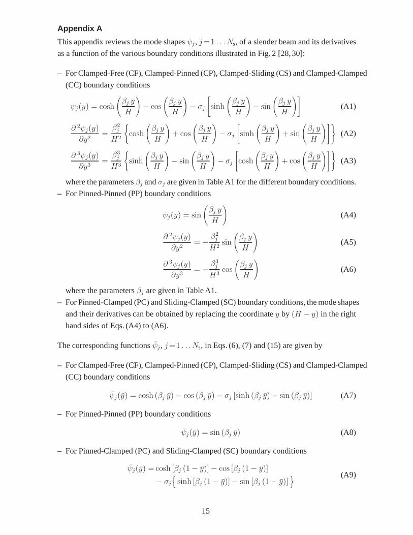
Appendix A

This appendix reviews the mode shapesψj , j=1 . . . Ns, of a slender beam and its derivatives

as a function of the various boundary conditions illustrated in Fig. 2 [28,30]:

– For Clamped-Free (CF), Clamped-Pinned (CP), Clamped-Sliding (CS) and Clamped-Clamped

(CC) boundary conditions

ψj(y) = cosh

(βj y

H

)− cos

(βj y

H

)− σj

[sinh

(βj y

H

)− sin

(βj y

H

)](A1)

∂ 2ψj(y)

∂y2=

β2j

H2

cosh

(βj y

H

)+ cos

(βj y

H

)− σj

[sinh

(βj y

H

)+ sin

(βj y

H

)](A2)

∂ 3ψj(y)

∂y3=

β3j

H3

sinh

(βj y

H

)− sin

(βj y

H

)− σj

[cosh

(βj y

H

)+ cos

(βj y

H

)](A3)

where the parametersβj andσj are given in Table A1 for the different boundary conditions.

– For Pinned-Pinned (PP) boundary conditions

ψj(y) = sin

(βj y

H

)(A4)

∂ 2ψj(y)

∂y2= −

β2j

H2sin

(βj y

H

)(A5)

∂ 3ψj(y)

∂y3= −

β3j

H3cos

(βj y

H

)(A6)

where the parametersβj are given in Table A1.

– For Pinned-Clamped (PC) and Sliding-Clamped (SC) boundaryconditions, the mode shapes

and their derivatives can be obtained by replacing the coordinatey by (H − y) in the right

hand sides of Eqs. (A4) to (A6).

The corresponding functionsψj , j=1 . . .Ns, in Eqs. (6), (7) and (15) are given by

– For Clamped-Free (CF), Clamped-Pinned (CP), Clamped-Sliding (CS) and Clamped-Clamped

(CC) boundary conditions

ψj(y) = cosh (βj y)− cos (βj y)− σj [sinh (βj y)− sin (βj y)] (A7)

– For Pinned-Pinned (PP) boundary conditions

ψj(y) = sin (βj y) (A8)

– For Pinned-Clamped (PC) and Sliding-Clamped (SC) boundaryconditions

ψj(y) = cosh [βj (1− y)]− cos [βj (1− y)]

− σjsinh [βj (1− y)]− sin [βj (1− y)]

(A9)

15

References

[1] H.M. Westergaard, Water pressures on dams during earthquakes. Transactions, ASCE 98 (1933)418–472.

[2] L.S. Jacobsen, Impulsive hydrodynamics of fluid inside acylindrical tank and of fluidsurrounding a cylindrical pier. Bulletin of the Seismological Society of America 39 (1949)189–1949.

[3] P.V. Rao, Calculation of added mass of circular and rectangular piers oscillating in water.Proceedingd of the Fifth Symposium of Earthquake Engineering (1974) 97.

[4] H. Goto, K. Toki, Vibrational characteristics and aseismic design of submerged bridge piers.Proceedings of the Third World Conference on Earthguake Engineering, Vol. II, New Zealand,1965 pp. 107–122.

[5] S. Kotsubo, Seismic force effect on submerged bridge piers with elliptic cross-sections.Proceedings of the Third World Conference on Earthguake Engineering, Vol. II, New Zealand,1965 pp. 342–356.

[6] A. K. Chopra, Earthquake behavior of reservoir-dam systems. Journal of the EngineeringMechanics Division, ASCE, 94, No. EM6, (1968) 1475–1500.

[7] A. K. Chopra, Earthquake response of concrete gravity dams. Journal of the EngineeringMechanics Division, ASCE, 96, No. EM4, (1970) 443–454.

[8] O.C. Zienkiewicz, R.E. Newton, Coupled vibration of a structure submerged in a compressiblefluid. Proceedings of the International Symposium of FiniteElement Techniques, Vol. 15, 1969,pp. 1-–15.

[9] A.R. Chardrasekaran, S.S. Saini, M.M. Malhotra, Hydrodynamic pressure on circularcylindrical cantilever structures surrounded by water. Fourth Symposium on EarthquakeEngineering, Roorkee, India, 1970, pp. 161–171.

[10] C.Y. Liaw, A.K. Chopra, Dynamics of towers surrounded by water. International JournalEarthquake Engineering and Structural Dynamics 3 (1974), no. 1, 33—49.

[11] Y. Tanaka, R. T. Hudspeth, Restoring forces on verticalcircular cylinders forced by earthquakes.International Journal Earthquake Engineering and Structural Dynamics 16 (1988), no. 1, 99—119.

[12] Han, R.P.S., Xu, H, Simple and accurate added mass modelfor hydrodynamic fluid-structureinteraction analysis. Journal of the Franklin Institute 333B (1996), no. 6, 929–945.

[13] K. Nagaya, Transient response in flexure to general uni-directional loads of variable cross-section beam with concentrated tip inertias immersed in a fluid. Journal of Sound and Vibration99 (1985), no. 3, 361-–378.

[14] A. Uscilowska, J.A. Kolodziej, Free vibration of immersed column carrying a tip mass. Journalof Sound and Vibration 216 (1998), 147-–157.

[15] H.R. Oz, Natural frequenciesof an immersed beam carrying a tip mass with rotatory inertia.Journal of Sound and Vibration 266 (2003) 1099-–1108.

16

[16] J.S. Wu, S.-H. Hsu, A unified approach for the free vibration analysis of an elastically supportedimmersed uniform beam carrying an eccentric tip mass with rotary inertia. Journal of Sound andVibration 291 (2006), 1122–1147.

[17] J.S. Wu, K.-W. Chen, An alternative approach to the structural motion analysis of wedge-beamoffshore structures supporting a load. Ocean Engineering 30 (2003), 1791–1806.

[18] Chang, J.Y., Liu, W.H, Some studies on the natural frequencies of immersed restrained column.Journal of Sound and Vibration, 130 (1989), no. 3, 516–524.

[19] Nagaya, K., Hai, Y., Seismic response of underwater members of variable cross section. Journalof Sound Vibration 103 (1985), 119–138.

[20] Xing, J.T., Price, W.G., Pomfret, M. J., Yam, L.H, Natural vibration of a beam-water interactionsystem. Journal of Sound and Vibration, 199 (1997), 491–512.

[21] S. Zhao, J.T. Xing, W.G. Price, Natural vibration of a flexible beam–water coupled system witha concentrated mass attached at the free end of the beam. Proceedings of the Institution ofMechanical Engineers, Part M: Journal of Engineering for the Maritime Environment, Vol. 216,no. 2, 2002, pp. 145–154.

[22] J.T. Xing, Natural vibration of two-dimensional slender structure–water interaction systemssubject to Sommerfeld radiation condition. Journal of Sound and Vibration 308 (2007) 67-–79.

[23] J. Nasserzare, Y. Lei, S. Eskandari-Shiri, Computation of natural frequencies and mode shapesof arch dams as an inverse problem. Advances in Engineering Software 31 (2000), no.11, 827–836

[24] S.M. de Souza, L.J. Pedroso, Study of flexible wall acoustic cavities using Beam Finite Element.Mechanics of Solids in Brazil, Brazilian Society of Mechanical Sciences and Engineering, H.S.da Costa Mattos & Marcílio Alves (Editors), 2009, pp. 223–237.

[25] G. Fenves, A.K. Chopra, Earthquake analysis and response of concrete gravity dams. ReportNo. UCB/EERC-84/10, University of California, Berkeley, California, 1984.

[26] N. Bouaanani, F.Y. Lu, Assessment of potential-based fluid finite elements for seismic analysisof dam–reservoir systems Journal of Computers and Structures 87 (2009) 206–224.

[27] B. Miquel, N. Bouaanani, Simplified evaluation of the vibration period and seismic response ofgravity dam-water systems Journal of Engineering Structures 32 (2010) 2488–2502.

[28] D. Young, R. P., Jr. Felgar, Tables of characteristic functions representing normal modes ofvibration of a beam. Engineering Research Series No. 44, Bureau of Engineering Research,Austin, Texas, 1949.

[29] T. Chang, R. R. Craig, Normal modes of uniform beams. Journal of Enginering MechanicsDivision EM4(95) (1969), 1027—1031.

[30] Blevins RD. Formulas for natural frequency and mode shape. , Kriger publishing Company,Florida (1984) 296–297.

[31] Y. Tang, Numerical Evaluation of Uniform Beam Modes. Journal of Engineering Mechanics129 (2003), 1475–1477.

17

[32] Higham, N. J, Accuracy and stability of numerical algorithms (Second ed.) SIAM, 2002.

[33] MATLAB . The Mathworks, Inc., Natick, MA, USA, 2011.

[34] ADINA Theory and Modeling Guide. Report ARD 10-7. ADINAR & D, Inc., 2010.

[35] Everstine GC. A symmetric potential formulation for fluid-structure interaction. Journal ofSound and Vibration 79 (1981) 157–160.

[36] Olson LG, Bathe KJ. Analysis of fluid-structure interactions: a direct symmetric coupledformulation based on the fluid velocity potential. Computers and Structures 21 (1985) 21–32.

18

List of tables

Tab. A1: Equations to determineσj andβj for j=1 . . .Ns.

Tab. 1: Modal parameters for Clamped-Free (CF) beam configuration and modesj=1 . . .Ns.

Tab. 2: Modal parameters for Clamped-Pinned (CP) beam configuration and modesj =

1 . . .Ns.

Tab. 3: Modal parameters for Pinned-Clamped (PC) beam configuration and modesj =

1 . . .Ns.

Tab. 4: Modal parameters for Clamped-Sliding (CS) beam configuration and modesj =

1 . . .Ns.

Tab. 5: Modal parameters for Sliding-Clamped (SC) beam configuration and modesj =

1 . . .Ns.

Tab. 6: Modal parameters for Clamped-Clamped (CC) beam configuration and modesj =1 . . .Ns.

Tab. 7: Modal parameters for Pinned-Pinned (PP) beam configuration and modesj=1 . . . Ns.

Tab. 8: Wet to dry beam frequency ratios for concrete beam-water system.

Tab. 9: Wet to dry beam frequency ratios for steel beam-watersystem.

Table A1Equations to determine parametersσj andβj for modesj=1 . . . Ns.

Boundary conditions σj βj is solution for:

Clamped-Free (CF)sinh(βj)− sin(βj)

cosh(βj) + cos(βj)cos(βj) cosh(βj) + 1 = 0

Clamped-Pinned (CP)cosh(βj)− cos(βj)

sinh(βj)− sin(βj)tan(βj)− tanh(βj) = 0

Pinned-Clamped (PC)cosh(βj)− cos(βj)

sinh(βj)− sin(βj)tan(βj)− tanh(βj) = 0

Clamped-Sliding (CS)sinh(βj)− sin(βj)

cosh(βj) + cos(βj)tan(βj) + tanh(βj) = 0

Sliding-Clamped (SC)sinh(βj)− sin(βj)

cosh(βj) + cos(βj)tan(βj) + tanh(βj) = 0

Clamped-Clamped (CC)cosh(βj)− cos(βj)

sinh(βj)− sin(βj)cos(βj) cosh(βj)− 1 = 0

Pinned-Pinned (PP) – βj = j π

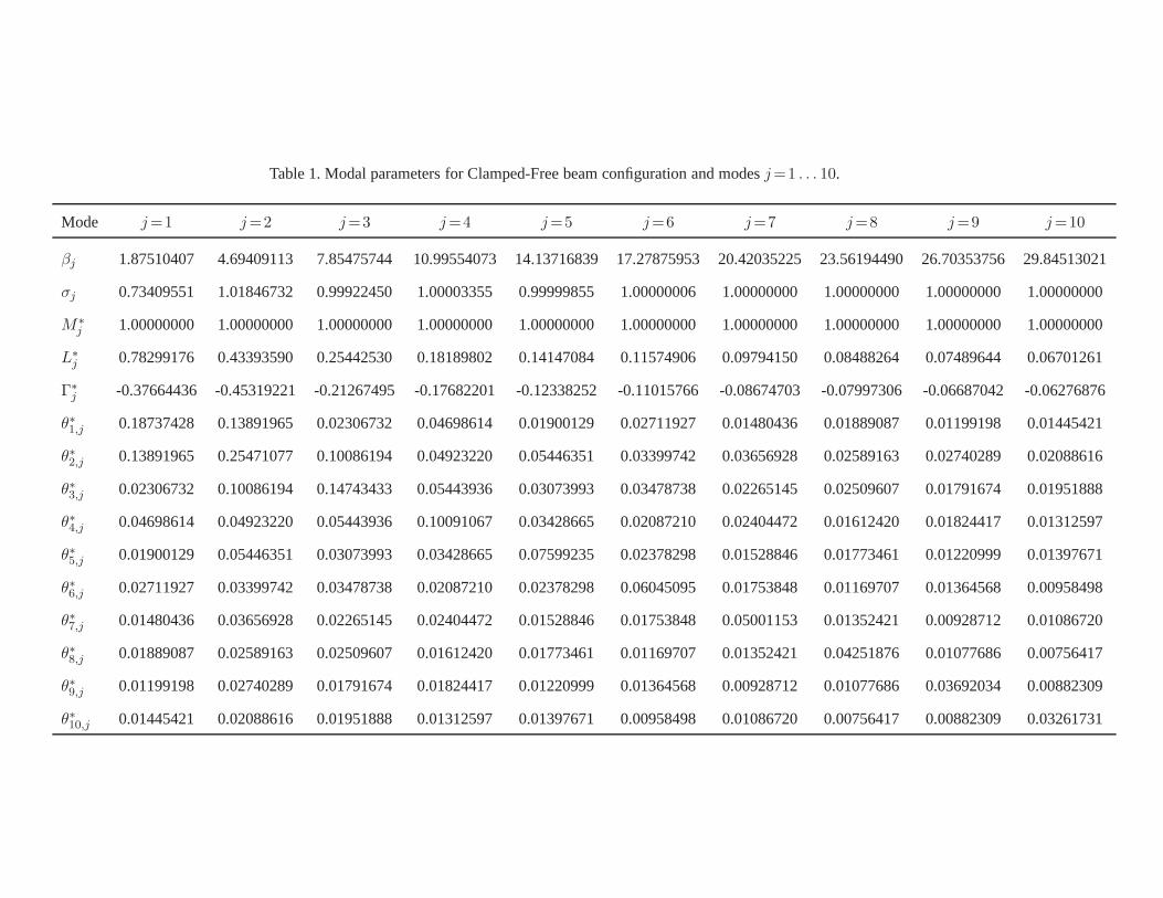
Table 1. Modal parameters for Clamped-Free beam configuration and modesj=1 . . . 10.

Mode j=1 j=2 j=3 j=4 j=5 j=6 j=7 j=8 j=9 j=10

βj 1.87510407 4.69409113 7.85475744 10.99554073 14.13716839 17.27875953 20.42035225 23.56194490 26.70353756 29.84513021

σj 0.73409551 1.01846732 0.99922450 1.00003355 0.99999855 1.00000006 1.00000000 1.00000000 1.00000000 1.00000000

M∗

j 1.00000000 1.00000000 1.00000000 1.00000000 1.00000000 1.00000000 1.00000000 1.00000000 1.00000000 1.00000000

L∗

j 0.78299176 0.43393590 0.25442530 0.18189802 0.14147084 0.11574906 0.09794150 0.08488264 0.07489644 0.06701261

Γ∗

j -0.37664436 -0.45319221 -0.21267495 -0.17682201 -0.12338252 -0.11015766 -0.08674703 -0.07997306 -0.06687042 -0.06276876

θ∗1,j 0.18737428 0.13891965 0.02306732 0.04698614 0.01900129 0.02711927 0.01480436 0.01889087 0.01199198 0.01445421

θ∗2,j 0.13891965 0.25471077 0.10086194 0.04923220 0.05446351 0.03399742 0.03656928 0.02589163 0.02740289 0.02088616

θ∗3,j 0.02306732 0.10086194 0.14743433 0.05443936 0.03073993 0.03478738 0.02265145 0.02509607 0.01791674 0.01951888

θ∗4,j 0.04698614 0.04923220 0.05443936 0.10091067 0.03428665 0.02087210 0.02404472 0.01612420 0.01824417 0.01312597

θ∗5,j 0.01900129 0.05446351 0.03073993 0.03428665 0.07599235 0.02378298 0.01528846 0.01773461 0.01220999 0.01397671

θ∗6,j 0.02711927 0.03399742 0.03478738 0.02087210 0.02378298 0.06045095 0.01753848 0.01169707 0.01364568 0.00958498

θ∗7,j 0.01480436 0.03656928 0.02265145 0.02404472 0.01528846 0.01753848 0.05001153 0.01352421 0.00928712 0.01086720

θ∗8,j 0.01889087 0.02589163 0.02509607 0.01612420 0.01773461 0.01169707 0.01352421 0.04251876 0.01077686 0.00756417

θ∗9,j 0.01199198 0.02740289 0.01791674 0.01824417 0.01220999 0.01364568 0.00928712 0.01077686 0.03692034 0.00882309

θ∗10,j 0.01445421 0.02088616 0.01951888 0.01312597 0.01397671 0.00958498 0.01086720 0.00756417 0.00882309 0.03261731

Table 2. Modal parameters for Clamped-Pinned beam configuration and modesj=1 . . . 10.

Mode j=1 j=2 j=3 j=4 j=5 j=6 j=7 j=8 j=9 j=10

βj 3.92660231 7.06858275 10.21017612 13.35176878 16.49336143 19.63495408 22.77654674 25.91813939 29.05973205 32.20132470

σj 1.00077731 1.00000145 1.00000000 1.00000000 1.00000000 1.00000000 1.00000000 1.00000000 1.00000000 1.00000000

M∗

j 1.00000000 1.00000000 1.00000000 1.00000000 1.00000000 1.00000000 1.00000000 1.00000000 1.00000000 1.00000000

L∗

j 0.86000091 0.08263119 0.33438600 0.04387308 0.20700531 0.02983386 0.14990040 0.02260141 0.11748951 0.01819138

Γ∗

j -0.57463863 -0.22387192 -0.19610132 -0.12740364 -0.11747947 -0.08877191 -0.08379277 -0.06808364 -0.06510595 -0.05520717

θ∗1,j 0.34894675 0.09636523 0.06874613 0.05303582 0.04307624 0.03623730 0.03126201 0.02748370 0.02451824 0.02212942

θ∗2,j 0.09636523 0.18069842 0.05207102 0.04099493 0.03360924 0.02840662 0.02456921 0.02163183 0.01931528 0.01744349

θ∗3,j 0.06874613 0.05207102 0.11733903 0.03252944 0.02700876 0.02299635 0.01997772 0.01763762 0.01577671 0.01426464

θ∗4,j 0.05303582 0.04099493 0.03252944 0.08546839 0.02239573 0.01922570 0.01679337 0.01488069 0.01334402 0.01208618

θ∗5,j 0.04307624 0.03360924 0.02700876 0.02239573 0.06663395 0.01644885 0.01444871 0.01285527 0.01156183 0.01049458

θ∗6,j 0.03623730 0.02840662 0.02299635 0.01922570 0.01644885 0.05432145 0.01264531 0.01129619 0.01019113 0.00927239

θ∗7,j 0.03126201 0.02456921 0.01997772 0.01679337 0.01444871 0.01264531 0.04569814 0.01005606 0.00909966 0.00829931

θ∗8,j 0.02748370 0.02163183 0.01763762 0.01488069 0.01285527 0.01129619 0.01005606 0.03934902 0.00820841 0.00750383

θ∗9,j 0.02451824 0.01931528 0.01577671 0.01334402 0.01156183 0.01019113 0.00909966 0.00820841 0.03449382 0.00684054

θ∗10,j 0.02212942 0.01744349 0.01426464 0.01208618 0.01049458 0.00927239 0.00829931 0.00750383 0.00684054 0.03066917

Table 3. Modal parameters for Pinned-Clamped beam configuration and modesj=1 . . . 10.

Mode j=1 j=2 j=3 j=4 j=5 j=6 j=7 j=8 j=9 j=10

βj 3.92660231 7.06858275 10.21017612 13.35176878 16.49336143 19.63495408 22.77654674 25.91813939 29.05973205 32.20132470

σj 1.00077731 1.00000145 1.00000000 1.00000000 1.00000000 1.00000000 1.00000000 1.00000000 1.00000000 1.00000000

M∗

j 1.00000000 1.00000000 1.00000000 1.00000000 1.00000000 1.00000000 1.00000000 1.00000000 1.00000000 1.00000000

L∗

j 0.86000091 0.08263119 0.33438600 0.04387308 0.20700531 0.02983386 0.14990040 0.02260141 0.11748951 0.01819138

Γ∗

j -0.65008940 0.07630378 -0.18764735 0.06077168 -0.10437260 0.04753510 -0.07134179 0.03871620 -0.05389119 0.03288874

θ∗1,j 0.42517390 -0.05350698 0.08215456 -0.03863831 0.04827983 -0.02921415 0.03392985 -0.02331070 0.02608839 -0.01953294

θ∗2,j -0.05350698 0.16093621 -0.02220990 0.02887463 -0.01573978 0.01957338 -0.01235525 0.01466114 -0.01016711 0.01167131

θ∗3,j 0.08215456 -0.02220990 0.11404365 -0.01510174 0.02319127 -0.01179012 0.01654423 -0.00971221 0.01275610 -0.00829536

θ∗4,j -0.03863831 0.02887463 -0.01510174 0.07776274 -0.01002847 0.01349708 -0.00781427 0.01030195 -0.00648317 0.00825628

θ∗5,j 0.04827983 -0.01573978 0.02319127 -0.01002847 0.06298601 -0.00757148 0.01130633 -0.00620408 0.00884611 -0.00531480

θ∗6,j -0.02921415 0.01957338 -0.01179012 0.01349708 -0.00757148 0.05001431 -0.00575588 0.00782770 -0.00473329 0.00637173

θ∗7,j 0.03392985 -0.01235525 0.01654423 -0.00781427 0.01130633 -0.00575588 0.04301687 -0.00464035 0.00679016 -0.00394881

θ∗8,j -0.02331070 0.01466114 -0.00971221 0.01030195 -0.00620408 0.00782770 -0.00464035 0.03654155 -0.00376882 0.00515097

θ∗9,j 0.02608839 -0.01016711 0.01275610 -0.00648317 0.00884611 -0.00473329 0.00679016 -0.00376882 0.03250581 -0.00317360

θ∗10,j -0.01953294 0.01167131 -0.00829536 0.00825628 -0.00531480 0.00637173 -0.00394881 0.00515097 -0.00317360 0.02868411

Table 4. Modal parameters for Clamped-Sliding beam configuration and modesj=1 . . . 10.

Mode j=1 j=2 j=3 j=4 j=5 j=6 j=7 j=8 j=9 j=10

βj 2.36502037 5.49780392 8.63937983 11.78097245 14.92256510 18.06415776 21.20575041 24.34734307 27.48893572 30.63052837

σj 0.98250221 0.99996645 0.99999994 1.00000000 1.00000000 1.00000000 1.00000000 1.00000000 1.00000000 1.00000000

M∗

j 1.00000000 1.00000000 1.00000000 1.00000000 1.00000000 1.00000000 1.00000000 1.00000000 1.00000000 1.00000000

L∗

j 0.83086152 0.36376941 0.23149808 0.16976527 0.13402522 0.11071648 0.09431404 0.08214449 0.07275655 0.06529434

Γ∗

j -0.43286638 -0.42564791 -0.16756712 -0.18178678 -0.10517939 -0.11405106 -0.07681829 -0.08275793 -0.06056673 -0.06482797

θ∗1,j 0.22689238 0.14212397 0.02072279 0.05815096 0.01755383 0.03503476 0.01429268 0.02471378 0.01195579 0.01896470

θ∗2,j 0.14212397 0.25076545 0.08206426 0.05438069 0.04980423 0.03590995 0.03522013 0.02682757 0.02711837 0.02144159

θ∗3,j 0.02072279 0.08206426 0.12952878 0.04471812 0.02614002 0.02964005 0.01930793 0.02189888 0.01525828 0.01727970

θ∗4,j 0.05815096 0.05438069 0.04471812 0.09818121 0.02975176 0.02178165 0.02172608 0.01650675 0.01694890 0.01325951

θ∗5,j 0.01755383 0.04980423 0.02614002 0.02975176 0.07140048 0.02081032 0.01423315 0.01578391 0.01135808 0.01262290

θ∗6,j 0.03503476 0.03590995 0.02964005 0.02178165 0.02081032 0.05910759 0.01569605 0.01208765 0.01246242 0.00980901

θ∗7,j 0.01429268 0.03522013 0.01930793 0.02172608 0.01423315 0.01569605 0.04808431 0.01217323 0.00894149 0.00987213

θ∗8,j 0.02471378 0.02682757 0.02189888 0.01650675 0.01578391 0.01208765 0.01217323 0.04176229 0.00981895 0.00779709

θ∗9,j 0.01195579 0.02711837 0.01525828 0.01694890 0.01135808 0.01246242 0.00894149 0.00981895 0.03589457 0.00805705

θ∗10,j 0.01896470 0.02144159 0.01727970 0.01325951 0.01262290 0.00980901 0.00987213 0.00779709 0.00805705 0.03209606

Table 5. Modal parameters for Sliding-Clamped beam configuration and modesj=1 . . . 10.

Mode j=1 j=2 j=3 j=4 j=5 j=6 j=7 j=8 j=9 j=10

βj 2.36502037 5.49780392 8.63937983 11.78097245 14.92256510 18.06415776 21.20575041 24.34734307 27.48893572 30.63052837

σj 0.98250221 0.99996645 0.99999994 1.00000000 1.00000000 1.00000000 1.00000000 1.00000000 1.00000000 1.00000000

M∗

j 1.00000000 1.00000000 1.00000000 1.00000000 1.00000000 1.00000000 1.00000000 1.00000000 1.00000000 1.00000000

L∗

j 0.83086152 0.36376941 0.23149808 0.16976527 0.13402522 0.11071648 0.09431404 0.08214449 0.07275655 0.06529434

Γ∗

j -0.68350770 -0.17189508 -0.07913826 -0.04607007 -0.03038167 -0.02165278 -0.01627248 -0.01271008 -0.01022374 -0.00842479

θ∗1,j 0.49079872 0.04802871 0.02127759 0.01179377 0.00745121 0.00512170 0.00373253 0.00283919 0.00223181 0.00180488

θ∗2,j 0.04802871 0.16975665 0.01534789 0.00949173 0.00633431 0.00448987 0.00333420 0.00256760 0.00203526 0.00165744

θ∗3,j 0.02127759 0.01534789 0.10157987 0.00743933 0.00533273 0.00395149 0.00302040 0.00237210 0.00190658 0.00155919

θ∗4,j 0.01179377 0.00949173 0.00743933 0.07236825 0.00437216 0.00339546 0.00268245 0.00215711 0.00176407 0.00146769

θ∗5,j 0.00745121 0.00633431 0.00533273 0.00437216 0.05617515 0.00287253 0.00234443 0.00193246 0.00161049 0.00135661

θ∗6,j 0.00512170 0.00448987 0.00395149 0.00339546 0.00287253 0.04589287 0.00202983 0.00171330 0.00145510 0.00124530

θ∗7,j 0.00373253 0.00333420 0.00302040 0.00268245 0.00234443 0.00202983 0.03878766 0.00150988 0.00130561 0.00113294

θ∗8,j 0.00283919 0.00256760 0.00237210 0.00215711 0.00193246 0.00171330 0.00150988 0.03358532 0.00116677 0.00102810

θ∗9,j 0.00223181 0.00203526 0.00190658 0.00176407 0.00161049 0.00145510 0.00130561 0.00116677 0.02961224 0.00092819

θ∗10,j 0.00180488 0.00165744 0.00155919 0.00146769 0.00135661 0.00124530 0.00113294 0.00102810 0.00092819 0.02648024

Table 6. Modal parameters for Clamped-Clamped beam configuration and modesj=1 . . . 10.

Mode j=1 j=2 j=3 j=4 j=5 j=6 j=7 j=8 j=9 j=10

βj 4.73004074 7.85320462 10.99560784 14.13716549 17.27875966 20.42035225 23.56194490 26.70353756 29.84513021 32.98672286

σj 0.98250221 1.00077731 0.99996645 1.00000145 0.99999994 1.00000000 1.00000000 1.00000000 1.00000000 1.00000000

M∗

j 1.00000000 1.00000000 1.00000000 1.00000000 1.00000000 1.00000000 1.00000000 1.00000000 1.00000000 1.00000000

L∗

j 0.83086152 0.00000000 0.36376941 0.00000000 0.23149808 0.00000000 0.16976527 0.00000000 0.13402522 0.00000000

Γ∗

j -0.59868962 -0.13987318 -0.21855053 -0.09614570 -0.12945024 -0.07230322 -0.09122754 -0.05783276 -0.07018707 -0.04817068

θ∗1,j 0.37372242 0.06778702 0.08798799 0.04552238 0.05315634 0.03375798 0.03774868 0.02674651 0.02919134 0.02212455

θ∗2,j 0.06778702 0.15976063 0.03574881 0.03706915 0.02434856 0.02570896 0.01848378 0.01946197 0.01489814 0.01560600

θ∗3,j 0.08798799 0.03574881 0.11879885 0.02488654 0.03088926 0.01879745 0.02242843 0.01505866 0.01745499 0.01252814

θ∗4,j 0.04552238 0.03706915 0.02488654 0.08161727 0.01729534 0.01907456 0.01329269 0.01474782 0.01079770 0.01194277

θ∗5,j 0.05315634 0.02434856 0.03088926 0.01729534 0.06695049 0.01322241 0.01616154 0.01067716 0.01279461 0.00889309

θ∗6,j 0.03375798 0.02570896 0.01879745 0.01907456 0.01322241 0.05304073 0.01024572 0.01156979 0.00836101 0.00950373

θ∗7,j 0.03774868 0.01848378 0.02242843 0.01329269 0.01616154 0.01024572 0.04583325 0.00832049 0.01008492 0.00692673

θ∗8,j 0.02674651 0.01946197 0.01505866 0.01474782 0.01067716 0.01156979 0.00832049 0.03878603 0.00677053 0.00782252

θ∗9,j 0.02919134 0.01489814 0.01745499 0.01079770 0.01279461 0.00836101 0.01008492 0.00677053 0.03435888 0.00561147

θ∗10,j 0.02212455 0.01560600 0.01252814 0.01194277 0.00889309 0.00950373 0.00692673 0.00782252 0.00561147 0.02965831

Table 7. Modal parameters for Pinned-Pinned beam configuration and modesj=1 . . . 10.

Mode j=1 j=2 j=3 j=4 j=5 j=6 j=7 j=8 j=9 j=10

βj 3.14159265 6.28318531 9.42477796 12.56637061 15.70796327 18.84955592 21.99114858 25.13274123 28.27433388 31.41592654

M∗

j 0.50000000 0.50000000 0.50000000 0.50000000 0.50000000 0.50000000 0.50000000 0.50000000 0.50000000 0.50000000

L∗

j 0.63661977 0.00000000 0.21220659 0.00000000 0.12732395 0.00000000 0.09094568 0.00000000 0.07073553 0.00000000

Γ∗

j -0.45071585 -0.11925463 -0.11251300 -0.06569036 -0.06362745 -0.04530423 -0.04431800 -0.03456940 -0.03399328 -0.02794578

θ∗1,j 0.20264237 0.04503164 0.03152215 0.02418842 0.01959948 0.01646314 0.01418643 0.01245973 0.01110584 0.01001614

θ∗2,j 0.04503164 0.09006327 0.01981392 0.01543942 0.01263337 0.01068283 0.00924963 0.00815278 0.00728676 0.00658589

θ∗3,j 0.03152215 0.01981392 0.05613944 0.01139576 0.00939231 0.00798396 0.00694015 0.00613585 0.00549732 0.00497825

θ∗4,j 0.02418842 0.01543942 0.01139576 0.04028953 0.00749098 0.00639410 0.00557609 0.00494253 0.00443741 0.00402531

θ∗5,j 0.01959948 0.01263337 0.00939231 0.00749098 0.03123378 0.00533858 0.00466794 0.00414652 0.00372942 0.00338815

θ∗6,j 0.01646314 0.01068283 0.00798396 0.00639410 0.00533858 0.02541751 0.00401713 0.00357494 0.00322029 0.00292945

θ∗7,j 0.01418643 0.00924963 0.00694015 0.00557609 0.00466794 0.00401713 0.02138386 0.00314341 0.00283535 0.00258224

θ∗8,j 0.01245973 0.00815278 0.00613585 0.00494253 0.00414652 0.00357494 0.00314341 0.01843053 0.00253352 0.00230969

θ∗9,j 0.01110584 0.00728676 0.00549732 0.00443741 0.00372942 0.00322029 0.00283535 0.00253352 0.01617910 0.00208975

θ∗10,j 0.01001614 0.00658589 0.00497825 0.00402531 0.00338815 0.00292945 0.00258224 0.00230969 0.00208975 0.01440835

Table 8. Wet to dry frequency ratios for concrete beam-watersystem.

Vibration mode number

Configuration Λf Ratio 1 2 3 4 5 6 7 8 9 10

CF 1 η(FE) 0.71 0.69 0.78 0.83 0.86 0.88 0.90 0.91 0.92 0.93η(PM) 0.71 0.69 0.78 0.83 0.86 0.89 0.90 0.91 0.92 0.93

2 η(FE) 0.58 0.58 0.67 0.73 0.77 0.81 0.83 0.85 0.86 0.88η(PM) 0.58 0.58 0.67 0.73 0.78 0.81 0.83 0.85 0.87 0.88

CP 1 η(FE) 0.59 0.73 0.80 0.85 0.87 0.89 0.91 0.92 0.93 0.93η(PM) 0.59 0.73 0.81 0.85 0.87 0.89 0.91 0.92 0.93 0.93

2 η(FE) 0.46 0.61 0.69 0.75 0.79 0.82 0.84 0.86 0.87 0.88η(PM) 0.46 0.61 0.70 0.75 0.79 0.82 0.84 0.86 0.87 0.88

PC 1 η(FE) 0.55 0.74 0.81 0.85 0.88 0.90 0.91 0.92 0.93 0.94η(PM) 0.56 0.74 0.81 0.85 0.88 0.90 0.91 0.92 0.93 0.94

2 η(FE) 0.43 0.61 0.70 0.75 0.79 0.82 0.84 0.86 0.87 0.88η(PM) 0.43 0.62 0.70 0.76 0.79 0.82 0.84 0.86 0.87 0.88

CS 1 η(FE) 0.67 0.69 0.79 0.83 0.87 0.89 0.90 0.91 0.92 0.93η(PM) 0.68 0.70 0.79 0.84 0.87 0.89 0.90 0.92 0.92 0.93

2 η(FE) 0.54 0.58 0.68 0.74 0.78 0.81 0.83 0.85 0.87 0.88η(PM) 0.54 0.58 0.68 0.74 0.78 0.81 0.83 0.85 0.87 0.88

SC 1 η(FE) 0.53 0.73 0.81 0.85 0.88 0.90 0.91 0.92 0.93 0.94η(PM) 0.53 0.73 0.81 0.85 0.88 0.90 0.91 0.92 0.93 0.94

2 η(FE) 0.40 0.60 0.70 0.75 0.79 0.82 0.84 0.86 0.87 0.89η(PM) 0.40 0.61 0.70 0.76 0.80 0.82 0.84 0.86 0.87 0.89

CC 1 η(FE) 0.58 0.74 0.80 0.85 0.87 0.89 0.91 0.92 0.93 0.93η(PM) 0.58 0.75 0.81 0.85 0.87 0.89 0.91 0.92 0.93 0.94

2 η(FE) 0.45 0.62 0.70 0.75 0.79 0.82 0.84 0.86 0.87 0.88η(PM) 0.45 0.62 0.70 0.75 0.79 0.82 0.84 0.86 0.87 0.89

PP 1 η(FE) 0.56 0.73 0.80 0.85 0.88 0.89 0.91 0.92 0.93 0.94η(PM) 0.57 0.73 0.81 0.85 0.88 0.90 0.91 0.92 0.93 0.94

2 η(FE) 0.43 0.60 0.69 0.75 0.79 0.82 0.84 0.86 0.87 0.88η(PM) 0.44 0.61 0.70 0.75 0.79 0.82 0.84 0.86 0.87 0.88

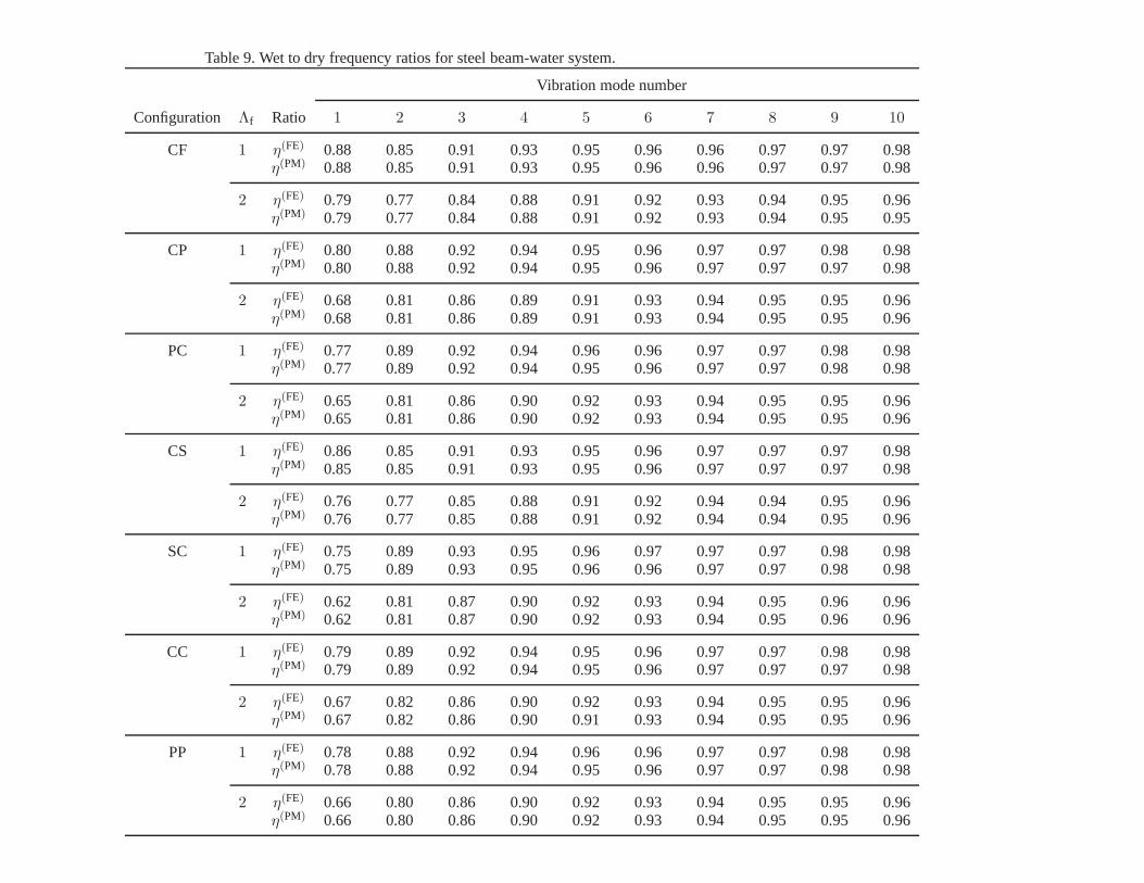
Table 9. Wet to dry frequency ratios for steel beam-water system.

Vibration mode number

Configuration Λf Ratio 1 2 3 4 5 6 7 8 9 10

CF 1 η(FE) 0.88 0.85 0.91 0.93 0.95 0.96 0.96 0.97 0.97 0.98η(PM) 0.88 0.85 0.91 0.93 0.95 0.96 0.96 0.97 0.97 0.98

2 η(FE) 0.79 0.77 0.84 0.88 0.91 0.92 0.93 0.94 0.95 0.96η(PM) 0.79 0.77 0.84 0.88 0.91 0.92 0.93 0.94 0.95 0.95

CP 1 η(FE) 0.80 0.88 0.92 0.94 0.95 0.96 0.97 0.97 0.98 0.98η(PM) 0.80 0.88 0.92 0.94 0.95 0.96 0.97 0.97 0.97 0.98

2 η(FE) 0.68 0.81 0.86 0.89 0.91 0.93 0.94 0.95 0.95 0.96η(PM) 0.68 0.81 0.86 0.89 0.91 0.93 0.94 0.95 0.95 0.96

PC 1 η(FE) 0.77 0.89 0.92 0.94 0.96 0.96 0.97 0.97 0.98 0.98η(PM) 0.77 0.89 0.92 0.94 0.95 0.96 0.97 0.97 0.98 0.98

2 η(FE) 0.65 0.81 0.86 0.90 0.92 0.93 0.94 0.95 0.95 0.96η(PM) 0.65 0.81 0.86 0.90 0.92 0.93 0.94 0.95 0.95 0.96

CS 1 η(FE) 0.86 0.85 0.91 0.93 0.95 0.96 0.97 0.97 0.97 0.98η(PM) 0.85 0.85 0.91 0.93 0.95 0.96 0.97 0.97 0.97 0.98

2 η(FE) 0.76 0.77 0.85 0.88 0.91 0.92 0.94 0.94 0.95 0.96η(PM) 0.76 0.77 0.85 0.88 0.91 0.92 0.94 0.94 0.95 0.96

SC 1 η(FE) 0.75 0.89 0.93 0.95 0.96 0.97 0.97 0.97 0.98 0.98η(PM) 0.75 0.89 0.93 0.95 0.96 0.96 0.97 0.97 0.98 0.98

2 η(FE) 0.62 0.81 0.87 0.90 0.92 0.93 0.94 0.95 0.96 0.96η(PM) 0.62 0.81 0.87 0.90 0.92 0.93 0.94 0.95 0.96 0.96

CC 1 η(FE) 0.79 0.89 0.92 0.94 0.95 0.96 0.97 0.97 0.98 0.98η(PM) 0.79 0.89 0.92 0.94 0.95 0.96 0.97 0.97 0.97 0.98

2 η(FE) 0.67 0.82 0.86 0.90 0.92 0.93 0.94 0.95 0.95 0.96η(PM) 0.67 0.82 0.86 0.90 0.91 0.93 0.94 0.95 0.95 0.96

PP 1 η(FE) 0.78 0.88 0.92 0.94 0.96 0.96 0.97 0.97 0.98 0.98η(PM) 0.78 0.88 0.92 0.94 0.95 0.96 0.97 0.97 0.98 0.98

2 η(FE) 0.66 0.80 0.86 0.90 0.92 0.93 0.94 0.95 0.95 0.96η(PM) 0.66 0.80 0.86 0.90 0.92 0.93 0.94 0.95 0.95 0.96

List of figures

Fig. 1: Slender beam vibrating in contact with a fluid acting on one or both sides.

Fig. 2: Studied beams-fluid configurations.

Fig. 3: Horizontal acceleration component of Imperial Valley earthquake (1940) at El Centro.

Fig. 4: Time-history responses for displacements, accelerations, shear forces, and overturn-ing bending moments of the concrete beam-fluid system.

Fig. 5: Time-history responses for displacements, accelerations, shear forces, and overturn-ing bending moments of the steel beam-fluid system.

Fig. 6: Time-history responses for displacements, accelerations, shear forces, and overturn-ing bending moments of the concrete beam-fluid system and thedry beam.

Fig. 7: Time-history responses for displacements, accelerations, shear forces, and overturn-ing bending moments of the steel beam-fluid system and the drybeam.

Fig. 8: Frequency response curves for accelerations of concrete and steel beam-fluid systems- CF configuration.

Fig. 9: Frequency response curves for accelerations of concrete beam-fluid systems.

Figure 1. Slender beam vibrating in contact with a fluid acting on: (a) one side, (b) both sides.

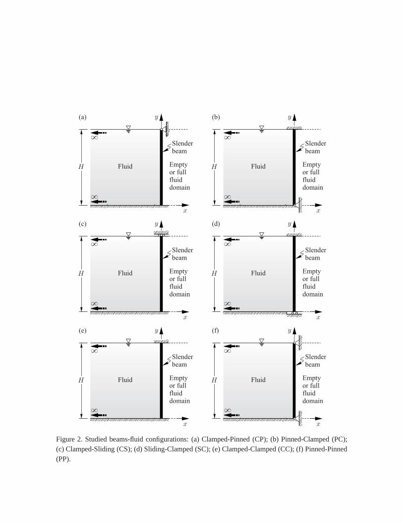
Figure 2. Studied beams-fluid configurations: (a) Clamped-Pinned (CP); (b) Pinned-Clamped (PC);(c) Clamped-Sliding (CS); (d) Sliding-Clamped (SC); (e) Clamped-Clamped (CC); (f) Pinned-Pinned(PP).

Figure 3. Horizontal acceleration component of Imperial Valley earthquake (1940) at El Centro.

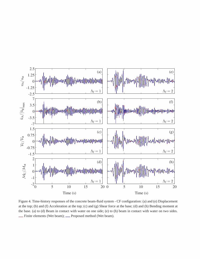
Figure 4. Time-history responses of the concrete beam-fluidsystem - CF configuration: (a) and (e) Displacementat the top; (b) and (f) Acceleration at the top; (c) and (g) Shear force at the base; (d) and (h) Bending moment atthe base. (a) to (d) Beam in contact with water on one side; (e)to (h) beam in contact with water on two sides.

Finite elements (Wet beam); Proposed method (Wet beam).

Figure 5. Time-history responses of the steel beam-fluid system - CF configuration: (a) and (e) Displacement atthe top; (b) and (f) Acceleration at the top; (c) and (g) Shearforce at the base; (d) and (h) Bending moment atthe base. (a) to (d) Beam in contact with water on one side; (e)to (h) beam in contact with water on two sides.

Finite elements (Wet beam); Proposed method (Wet beam).

Figure 6. Time-history responses of the concrete beam-fluidsystem - CF configuration: (a) and (e) Displacementat the top; (b) and (f) Acceleration at the top; (c) and (g) Shear force at the base; (d) and (h) Bending moment atthe base. (a) to (d) Beam in contact with water on one side; (e)to (h) beam in contact with water on two sides.

Finite elements (Wet beam); Proposed method (Wet beam). Proposed method (Dry beam).

Figure 7. Time-history responses of the steel beam-fluid system - CF configuration: (a) and (e) Displacement atthe top; (b) and (f) Acceleration at the top; (c) and (g) Shearforce at the base; (d) and (h) Bending moment atthe base. (a) to (d) Beam in contact with water on one side; (e)to (h) beam in contact with water on two sides.

Finite elements (Wet beam); Proposed method (Wet beam). Proposed method (Dry beam).

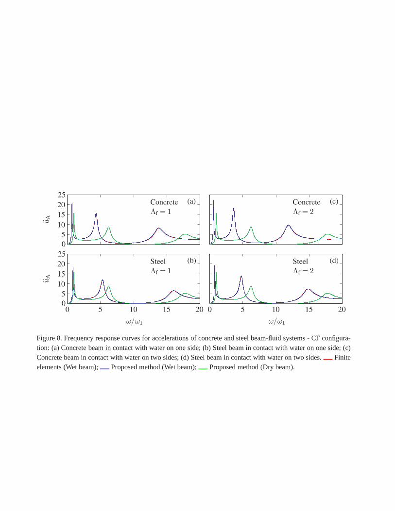
Figure 8. Frequency response curves for accelerations of concrete and steel beam-fluid systems - CF configura-tion: (a) Concrete beam in contact with water on one side; (b)Steel beam in contact with water on one side; (c)Concrete beam in contact with water on two sides; (d) Steel beam in contact with water on two sides. Finiteelements (Wet beam); Proposed method (Wet beam); Proposed method (Dry beam).

Figure 9. Frequency response curves for accelerations of concrete beam-fluid systems: (a) and (g) CP config-uration; (b) and (h) PC configuration; (c) and (i) CS configuration; (d) and (j) SC configuration; (e) and (k)CC configuration; (f) and (l) PP configuration. (a) to (f) Beamin contact with water on one side; (g) to (l)Beam in contact with water on two sides. Finite elements (Wet beam); Proposed method (Wet beam);

Proposed analytical method (Dry beam).