PHYSICAL REVIEW B 84, 205331 (2011)

Efficient simulation of multidimensional phonon transport using energy-based variance-reducedMonte Carlo formulations

Jean-Philippe M. Peraud and Nicolas G. HadjiconstantinouDepartment of Mechanical Engineering, Massachusetts Institute of Technology, Cambridge, Massachusetts 02139, USA

(Received 13 August 2011; published 21 November 2011)

We present a Monte Carlo method for obtaining solutions of the Boltzmann equation to describe phonontransport in micro- and nanoscale devices. The proposed method can resolve arbitrarily small signals (e.g.,temperature differences) at small constant cost and thus represents a considerable improvement compared totraditional Monte Carlo methods, whose cost increases quadratically with decreasing signal. This is achieved viaa control-variate variance-reduction formulation in which the stochastic particle description solves only for thedeviation from a nearby equilibrium, while the latter is described analytically. We also show that simulation of anenergy-based Boltzmann equation results in an algorithm that lends itself naturally to exact energy conservation,thereby considerably improving the simulation fidelity. Simulations using the proposed method are used toinvestigate the effect of porosity on the effective thermal conductivity of silicon. We also present simulationsof a recently developed thermal conductivity spectroscopy process. The latter simulations demonstrate how thecomputational gains introduced by the proposed method enable the simulation of otherwise intractable multiscalephenomena.

DOI: 10.1103/PhysRevB.84.205331 PACS number(s): 63.20.−e

I. INTRODUCTION

Over the past two decades, the dramatic advancesassociated with microelectromechanical systems (MEMS)and nanoelectromechanical systems (NEMS) have attractedsignificant attention to microscale and nanoscale heat transferconsiderations.1 Applications range from thermal manage-ment of electronic devices2 to the development of thermoelec-tric materials with higher figures of merit.3 The thermoelectricfigure of merit is proportional to the electrical conductivityand inversely proportional to the thermal conductivity andcan thus be improved by reducing the latter and/or increasingthe former. One of the most promising approaches towardreducing the thermal conductivity of thermoelectric materialsis the introduction of nanostructures that interact with theballistic motion of phonons at small scales, thus influencingheat transport.4 Such an approach requires a reliable descrip-tion of phonon transport at the nanoscale and cannot relyon Fourier’s law, which is valid for diffuse transport. Onthe other hand, first-principles calculations (e.g., moleculardynamics approaches, classical or quantum mechanical) aretoo expensive for treating phonon transport at the device (e.g.,micrometer) scale. At these scales, a kinetic description basedon the Boltzmann transport equation (BTE) offers a reasonablebalance between fidelity and model complexity and is able toaccurately describe the transition from diffusive to ballistictransport as characteristic system length scales approach andultimately become smaller than the phonon mean free path.

Solution of the BTE is a challenging task, especially incomplex geometries. The high dimensionality of the distri-bution function coupled with the ability of particle methodsto naturally simulate advection processes without stabilityproblems5 make particle Monte Carlo methods particularlyappealing. Following the development of the direct MonteCarlo method by Bird6 for treating dilute gases, MonteCarlo methods for phonon transport were first introducedby Peterson7 and subsequently improved by Mazumder and

Majumdar.8 Over the past decade, further important refine-ments have been introduced: Lacroix et al. introduced amethod to treat frequency-dependent mean free paths;9 Jenget al. introduced a method for efficiently treating transmissionand reflection of phonons at material interfaces and used thismethod to model the thermal conductivity of nanoparticlecomposites;4 Hao et al. developed10 a formulation for periodicboundary conditions in order to study the thermal conductivityof periodic nanoporous materials while simulating only oneunit cell (period).

The work presented here introduces a number of improve-ments which enable efficient and accurate simulation of themost challenging phonon transport problems, namely, threedimensional and transient. Accuracy is improved compared toprevious approaches by introducing an energy-based formu-lation, which simulates energy packets rather than phonons;this formulation makes energy conservation particularly easyto implement rigorously, in contrast to previous approacheswhich were ad hoc and in many cases ineffective. We alsointroduce a variance-reduced formulation for substantiallyreducing the statistical uncertainty associated with samplingsolution (temperature and heat flux) fields. This formulationis based on the concept of control variates, first introducedin the context of Monte Carlo solutions of the Boltzmannequation for dilute gases;5 it relies on the fact that signalstrength is intimately linked to deviation from equilibrium,or, in other words, that the large computational cost associatedwith small signals is due to the fact that in these problemsthe deviation from equilibrium is small. This observation canbe exploited by utilizing the nearby equilibrium state as a“control” and using the Monte Carlo method to calculatethe contribution of nonequilibrium therefrom. Because thedeviation from equilibrium is small, only a small quantityis evaluated stochastically (the fields associated with theequilibrium component are known analytically), resulting insmall statistical uncertainty; moreover, the latter decreases as

205331-11098-0121/2011/84(20)/205331(15) ©2011 American Physical Society

PERAUD AND HADJICONSTANTINOU PHYSICAL REVIEW B 84, 205331 (2011)

the deviation from equilibrium decreases, thus enabling thesimulation of arbitrarily small deviations from equilibrium.

In the technique presented here, we use particles to simulatethe deviation from equilibrium, and it is thus referred toas a deviational method; the origin of this methodologycan be found in the low-variance deviational simulationMonte Carlo method11–14 recently developed for dilute gases.The theoretical basis underlying this method as well as themodifications required for use in phonon transport simulationsare described in Sec. II C. The resulting algorithm is describedin Sec. III and validated in Sec. IV.

The proposed algorithm is used to obtain solutions to twoproblems of practical interest. The first application studies thethermal conductivity of porous silicon containing voids withdifferent degrees of alignment and is intended to showcase howballistic effects influence the “effective” thermal conductivity.The second application is related to the recently developed ex-perimental method of “thermal conductivity spectroscopy”15

based on the pump-probe technique known as transientthermoreflectance, which uses the response of a material tolaser irradiation to infer information about physical propertiesof interest16 (e.g., the mean free paths of the dominant heatcarriers).

II. THEORETICAL BASIS

A. Summary of traditional Monte Carlo simulation methods

We consider the Boltzmann transport equation in thefrequency-dependent relaxation-time approximation

∂f

∂t+ Vg(ω,p)∇f = − f − f loc

τ (ω,p,T ), (1)

where f = f (t,x,k,p) is the phonon distribution functionin phase space, ω = ω(k,p) the phonon radial frequency, p

the phonon polarization, and T the temperature; similarly tothe nomenclature adopted in Ref. 1, f is defined in referenceto the occupation number. For example, if the system isperfectly thermalized at temperature T , f is a Bose-Einsteindistribution,

feq

T = 1

exp(

hω(k,p)kbT

) − 1, (2)

where kb is Boltzmann’s constant. Also, f loc is an equilib-rium (Bose-Einstein) distribution parametrized by the localpseudotemperature defined more precisely in Sec. II A 2.

In this work we consider longitudinal acoustic (LA),transverse acoustic (TA), longitudinal optical (LO), andtransverse optical (TO) polarizations; acoustic phonons areknown to be the most important contributors to lattice thermalconductivity.17,18 The phonon radial frequency is given by thedispersion relation ω = ω(k,p). Phonons travel at the groupvelocity Vg = ∇kω.

In the following, we always consider the ideal case wherethe dispersion relation is isotropic. For convenience, the radialfrequency ω and two polar angles θ and φ are usually preferredas primary parameters compared to the wave vector. Equation(1) is simulated using computational particles that representphonon bundles, namely, collections of phonons with similar

characteristics (the position vector x, the wave vector k, and thepolarization or propagation mode p), using the approximation

1

8π3f (t,x,k,p) ≈ Neff

∑i

δ3(x − xi)δ3(k − ki)δp,pi

, (3)

where xi , ki , and pi respectively represent the position, thewave vector, and the polarization of particle i and Neff isthe number of phonons in each phonon bundle. The factor1/8π3 is necessary for converting the quantity representing theoccupation number, f , into a quantity representing the phonondensity in phase space. Written in polar coordinates, and usingthe frequency instead of the wave number, this expressionbecomes

D(ω,p)

4πf (t,x,ω,θ,φ,p) sin(θ )

≈ Neff

∑i

δ3(x − xi)δ(ω − ωi)δ(θ − θi)δ(φ − φi)δp,pi,

(4)

where ωi , θi , and φi respectively represent the radial frequency,the polar angle, and the azimuthal angle of particle i. Thedensity of states D(ω,p) is made necessary by the use of ω asa primary parameter and is given by

D(ω,p) = k(ω,p)2

2π2Vg(ω,p). (5)

1. Initialization

Systems are typically initialized in an equilibrium state attemperature T ; the number of phonons in a given volume V iscalculated using the Bose-Einstein statistics

N = V

∫ ωmax

ω=0

∑p

D(ω,p)f eq

T (ω)dω, (6)

where ωmax is the maximum (cutoff) frequency and feq

T is theoccupation number at equilibrium at temperature T .

The number of computational particles (each representinga phonon bundle) is given by N/Neff . The value of Neff

is determined by balancing computational cost (includingstorage) with the need for a sufficiently large number ofparticles for statistically meaningful results.

2. Time integration

Once the system is initialized, the simulation proceeds byapplying a splitting algorithm with time step t . Integrationfor one time step is comprised of three substeps:

(1) The advection substep, during which bundle i moves byVg,it .

(2) The sampling substep, during which the temperature (T )and pseudotemperature (Tloc) are locally measured. They arecalculated by inverting the local energy (E) and pseudoenergy(E)10 relations,

E = Neff

∑i

hωi = V

∫ ωmax

ω=0

∑p

D(ω,p)hω

exp(

hωkbT

) − 1dω (7)

205331-2

EFFICIENT SIMULATION OF MULTIDIMENSIONAL . . . PHYSICAL REVIEW B 84, 205331 (2011)

and

E = Neff

∑i

hωi

τ (ωi,pi,T )

= V

∫ ωmax

ω=0

∑p

D(ω,p)hω

τ (ω,p,T )

1

exp(

hωkbTloc

) − 1dω, (8)

respectively.(3) The scattering substep, during which each phonon i is

scattered according to its scattering probability given by

Pi = 1 − exp

(− t

τ (ωi,pi,T )

). (9)

Scattering proceeds by drawing new frequencies, polariza-tions, and traveling directions. Because of the frequency-dependent relaxation times, frequencies must be drawnfrom the distribution D(ω,p)f loc/τ (ω,p,T ). Since scatteringevents conserve energy, the latter must be conserved duringthis substep. However, because the frequencies of the scatteredphonons are drawn randomly, conservation of energy isenforced by adding or deleting particles until a target energyis approximately reached.8,9 In addition to being approximate,this method does not always ensure that energy is conserved,resulting in random walks in the energy of the simulatedsystem, which in some cases leads to deterministic error. Inthe next section, we present a convenient way for rigorouslyconserving energy.

B. Energy-based formulation

While most computational techniques developed so farconserve energy in only an approximate manner,8,9 here weshow that an energy-based formulation provides a convenientand rigorous way to conserve energy in the relaxation timeapproximation.

Adopting a similar approach as in Ref. 2 to derive theequation of phonon radiative transfer, we multiply (1) by hω

to obtain

∂e

∂t+ Vg∇e = eloc − e

τ, (10)

which we will refer to as the energy-based BTE. Here, e = hωf

and eloc = hωf loc. Equation (10) can be simulated by writing

e ≈ 8π3Eeff

∑i

δ3(x − xi)δ3(k − ki)δp,pi

, (11)

where Eeff is defined as the effective energy carried by eachcomputational particle. Statement (11) defines computationalparticles that all represent the same amount of energy. Fromthe point of view of phonons, comparison of (3) and (11)shows that the effective number of phonons represented by thenewly defined particles is variable and is linked to the effectiveenergy by the relation Eeff = Neffhω. By analogy with thedescription of Sec. II A, computational particles defined by(11) obey the same computational rules as in the previousMonte Carlo approaches. Modifications appear at three levels:

(1) When drawing particle frequencies during initialization,emission from boundaries, or scattering, the distribution func-tions that we use must account for the factor hω. For example,when initializing an equilibrium population of particles at

a temperature T , one has to draw the frequencies from thedistribution

hω∑

p D(ω,p)

exp(

hωkbT

) − 1. (12)

(2) Calculation of the energy in a cell is straightforwardand simply consists in counting the number of computationalparticles. The energy associated with N particles is given byEeffN .

(3) Since the energy in a cell is proportional to the numberof particles, there is no need for an addition or deletionprocess: energy is strictly and automatically conserved bysimply conserving the number of particles.

C. Deviational formulation

In this section we introduce an additional modificationwhich dramatically decreases the statistical uncertainty as-sociated with Monte Carlo simulations of (10). Our approachbelongs to a more general class of control-variate variance-reduction methods for solving kinetic equations,5,11,19 in whichthe moments 〈R〉 of a given distribution f are computed bywriting∫

Rf dxdc =∫

R(f − f eq)dxdc +∫

Rf eqdxdc, (13)

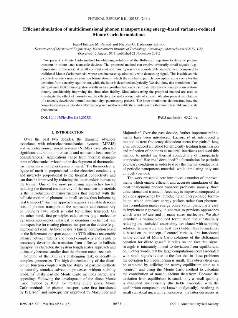
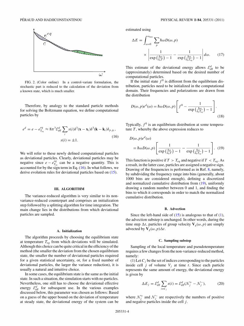
where the first term of the right-hand side is computed stochas-tically and the second term is computed deterministically. Iff eq ≈ f , the variance reduction is large because only a smallterm is determined stochastically (see Figs. 1 and 2).

In the present context, this methodology provides signif-icant computational savings when an equilibrium (constant-temperature) state exists nearby, which is precisely the regimein which statistical noise becomes problematic (low signals).The degree of variance reduction achieved by this method isquantified in Sec. V.

Let

eeq

Teq(ω) = hω

exp(

hωkbTeq

) − 1, (14)

where Teq �= Teq(x,t). Then, it is straightforward to show thated = e − e

eq

Teqis governed by

∂ed

∂t+ Vg∇ed =

(eloc − e

eq

Teq

) − ed

τ. (15)

FIG. 1. (Color online) In standard particle methods, the momentsof the distribution are stochastically integrated.

205331-3

PERAUD AND HADJICONSTANTINOU PHYSICAL REVIEW B 84, 205331 (2011)

+ +

- -

FIG. 2. (Color online) In a control-variate formulation, thestochastic part is reduced to the calculation of the deviation froma known state, which is much smaller.

Therefore, by analogy to the standard particle methodsfor solving the Boltzmann equation, we define computationalparticles by

ed = e − eeq

Teq≈ 8π3Ed

eff

∑i

s(i)δ3(x − xi)δ3(k − ki)δp,pi

,

(16)s(i) = ±1.

We will refer to these newly defined computational particlesas deviational particles. Clearly, deviational particles may benegative since e − e

eq

Teqcan be a negative quantity. This is

accounted for by the sign term in Eq. (16). In what follows, wederive evolution rules for deviational particles based on (15).

III. ALGORITHM

The variance-reduced algorithm is very similar to its non-variance-reduced counterpart and comprises an initializationstep followed by a splitting algorithm for time integration. Themain change lies in the distributions from which deviationalparticles are sampled.

A. Initialization

The algorithm proceeds by choosing the equilibrium stateat temperature Teq from which deviations will be simulated.Although this choice can be quite critical in the efficiency of themethod (the smaller the deviation from the chosen equilibriumstate, the smaller the number of deviational particles requiredfor a given statistical uncertainty, or, for a fixed number ofdeviational particles, the larger the variance reduction), it isusually a natural and intuitive choice.

In some cases, the equilibrium state is the same as the initialstate. In such a situation, the simulation starts with no particles.Nevertheless, one still has to choose the deviational effectiveenergy Ed

eff for subsequent use. In the various examplesdiscussed below, this parameter was chosen as follows: Basedon a guess of the upper bound on the deviation of temperatureat steady state, the deviational energy of the system can be

estimated using

E =∫ ωmax

ω=0

∑p

hωD(ω,p)

×∣∣∣∣∣ 1

exp(

hωkbT

) − 1− 1

exp(

hωkbTeq

) − 1

∣∣∣∣∣ dω. (17)

This estimate of the deviational energy allows Edeff to be

(approximately) determined based on the desired number ofcomputational particles.

If the initial state f 0 is different from the equilibrium dis-tribution, particles need to be initialized in the computationaldomain. Their frequencies and polarizations are drawn fromthe distribution

D(ω,p)ed (ω) = hωD(ω,p)

[f 0 − 1

exp(

hωkbTeq

) − 1

].

(18)

Typically, f 0 is an equilibrium distribution at some tempera-ture T , whereby the above expression reduces to

D(ω,p)ed (ω)

= hωD(ω,p)

[1

exp(

hωkbT

) − 1− 1

exp(

hωkbTeq

) − 1

]. (19)

This function is positive if T > Teq and negative if T < Teq . Asa result, in the latter case, particles are assigned a negative sign.Drawing of the frequencies is performed as in Ref. 8, namely,by subdividing the frequency range into bins (generally, about1000 bins are considered enough), defining a discretizedand normalized cumulative distribution from (19), uniformlydrawing a random number between 0 and 1, and finding thebins to which it corresponds in order to match the normalizedcumulative distribution.

B. Advection

Since the left-hand side of (15) is analogous to that of (1),the advection substep is unchanged. In other words, during thetime step t , particles of group velocity Vg(ω,p) are simplyadvected by Vg(ω,p)t .

C. Sampling substep

Sampling of the local temperature and pseudotemperaturerequires a few changes from the non-variance-reduced method,namely:

(1) Let Cj be the set of indices corresponding to the particlesinside cell j of volume Vj at time t . Since each particlerepresents the same amount of energy, the deviational energyis given by

Ej = Edeff

∑i∈Cj

s(i) = Edeff(N+

j − N−j ), (20)

where N+j and N−

j are respectively the numbers of positiveand negative particles inside the cell j .

205331-4

EFFICIENT SIMULATION OF MULTIDIMENSIONAL . . . PHYSICAL REVIEW B 84, 205331 (2011)

(2) The corresponding temperature Tj is then calculated bynumerically inverting the expression

Ej

Vj

=∫ ωmax

ω=0

∑p

D(ω,p)hω

×[

1

exp(

hωkbTj

) − 1− 1

exp(

hωkbTeq

) − 1

]dω. (21)

(3) Similarly, once Tj is known, the deviational pseudoen-ergy is computed using

Ej = Edeff

∑i∈Cj

s(i)

τ (ωi,pi,Tj ). (22)

(4) The corresponding pseudotemperature [Tloc]j is calcu-lated by numerically inverting

Ej

Vj

=∫ ωmax

ω=0

∑p

D(ω,p)hω

τ (ω,p,Tj )

×[

1

exp(

hωkb[Tloc]j

) − 1− 1

exp(

hωkbTeq

) − 1

]dω.

(23)

D. Scattering step

During the scattering step we integrate

ded

dt=

(eloc − e

eq

Teq

) − ed

τ (ω,p,Tj )(24)

for a time step t , where

eloc − eeq

Teq= hω

[1

exp(

hωkb[Tloc]j

) − 1− 1

exp(

hωkbTeq

) − 1

].

(25)

We select the particles to be scattered according to thescattering probability (specific to each particle’s frequencyand polarization, and depending on the local temperature)

P (ωi,pi,Tj ) = 1 − exp

(− t

τ (ωi,pi,Tj )

). (26)

The pool of selected particles represents a certain amount ofdeviational energyEd

eff (N+s,j − N−

s,j ), whereN+s,j andN−

s,j referrespectively to the numbers of positive and negative selected(i.e., scattered) particles in cell j . This pool of selected particlesmust be replaced by particles with properties drawn from thedistribution

D(ω,p)(eloc − e

eq

Teq

)τ (ω,p,Tj )

= D(ω,p)hω

τ (ω,p,Tj )

(1

exp(

hωkb[Tloc]j

) − 1− 1

exp(

hωkbTeq

) − 1

),

(27)

which is either positive for all frequencies and polarizations ornegative for all frequencies and polarizations. In other words,scattered particles must be replaced by particles which all

have the same sign as eloc − eeq

Teqand which respect the energy

conservation requirement. Therefore, out of the N+s,j + N−

s,j

selected particles, we redraw properties for |N+s,j − N−

s,j | ofthem according to the distribution (27) and delete the otherselected particles. The |N+

s,j − N−s,j | particles to be kept are

chosen randomly inside the cell j and are given the sign ofeloc − e

eq

Teq.

This process tends to reduce the number of particlesin the system and counteracts sources of particle creationwithin the algorithm (e.g., see the boundary conditionsdiscussed in the next section). A bounded number of particlesis essential to the method stability, and the reduction processjust described is a major contributor to the latter.11,12 Hence,in a typical problem starting from an equilibrium state that isalso chosen as the control, the number of particles will firstincrease from zero and, at steady state, reach a constant valuethat can be estimated by appropriate choice of Ed

eff as describedin Sec. III A. The constant value will usually be higher than(but of the same order as) the estimated value: indeed, the rateof elimination of pairs of particles of opposite signs dependson the number of particles per cell and therefore on the spatialdiscretization chosen (the finer the discretization, the smallerthe number of particles per cell and therefore the smaller therate of elimination).

E. Boundary conditions

In phonon transport problems, various types of boundarycondition appear. Isothermal boundary conditions, similar bynature to a blackbody, have been used in several studies.8,9 Adi-abatic boundaries also naturally appear.8,20 Recently, a classof periodic boundary conditions has also been introduced.10

The deviational formulation adapts remarkably well to thesedifferent classes of boundary conditions.

1. Adiabatic boundaries

Adiabatic boundaries reflect all incident phonons. Thisreflection process can be divided into two main categories:diffuse and specular reflection. In both cases, it is assumedthat the polarization and frequency remain the same when aphonon is reflected. The only modified parameter during theprocess is the traveling direction.

(i) Specular reflection on a boundary ∂n of normal vectorn can be expressed, in terms of the energy distribution, by

e(x,k) = e(x,k′), (28)

where k′ = k − 2(k · n)n and x ∈ ∂n. Since the equilibriumdistribution e

eq

Teqis isotropic, then substracting it from both

sides simply yields

ed (x,k) = ed (x,k′). (29)

In other words, deviational particles are specularly reflected.(ii) Diffuse reflection amounts to randomization of the

traveling direction of a phonon incident on the boundary, inorder for the population of phonons leaving the boundaryto be isotropic. Since an equilibrium distribution is alreadyisotropic, incident deviational particles are treated identicallyto real phonons.

205331-5

PERAUD AND HADJICONSTANTINOU PHYSICAL REVIEW B 84, 205331 (2011)

Periodicflux

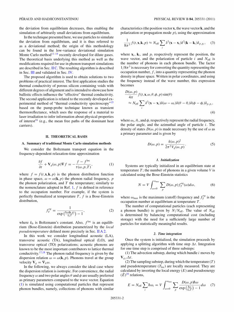
FIG. 3. (Color online) Example of a periodic nanostructure.Each periodic cell comprises two rectangular voids with diffuselyreflecting walls. This nanostructure, and in particular the influence ofthe parameter d , is studied further in Sec. VI A.

2. Isothermal boundaries

In the case of an isothermal boundary at temperature Tb,incident phonons are absorbed, while the boundary itself,at temperature Tb, emits new phonons from the equilibriumdistribution corresponding to Tb. The emitted heat flux perunit radial frequency is expressed by

q ′′ω,b = 1

4

∑p

D(ω,p)Vg(ω,p)hω

exp(

hωkbTb

) − 1. (30)

Subtracting the heat flux per unit radial frequency corre-sponding to a boundary at equilibrium temperature, we obtain

q ′′ω,b = 1

4

∑p

D(ω,p)Vg(ω,p)hω

×(

1

exp(

hωkbTb

) − 1− 1

exp(

hωkbTeq

) − 1

), (31)

which gives the frequency distribution of emitted particles.Traveling directions must be chosen accordingly, as explained,for example, in Ref. 8.

3. Periodic unit cell boundary conditions

Heat transfer in periodic nanostructures is a subject ofconsiderable interest in the context of many applications.Such nanostructures are considered by Hao et al.,10 by Huanget al.,21 and by Jeng et al.4 Hao et al. developed periodicboundary conditions that allow efficient simulation of suchstructures by considering only one unit cell (period). In this

section we review the work of Hao et al.10 and explain howthe deviational particle formulation presented here lends itselfnaturally to this type of boundary condition. Simulations usingthese boundary conditions are presented in Sec. VI A.

We consider the two-dimensional (2D) periodic structuredepicted in Fig. 3, in which square unit cells containing tworectangular voids are organized in a square lattice. Our interestfocuses on determining the effective thermal conductivity ofsuch a structure as a function of d, the degree of alignment.

The formulation introduced by Hao et al. amounts to statingthat, at the boundaries, the deviation of the phonon distributionfrom the local equilibrium is periodic. Using the notations fromFig. 3, this condition can be written as

f +1 − f

eq

T1= f +

2 − feq

T2,

f −1 − f

eq

T1= f −

2 − feq

T2,

(32)

where feq

T1and f

eq

T2refer to the equilibrium distributions at

temperatures T1 and T2, and the superscript + denotes particlesmoving to the right (with respect to Fig. 3) and the superscript− refers to particles moving to the left. This formulationenforces at the same time the periodicity of the heat fluxand a temperature gradient. In terms of deviational energydistributions, this relation becomes

hω(f +

1 − feq

Teq− f

eq

T1

) = hω(f +

2 − feq

Teq− f

eq

T2

),

hω(f −

1 − feq

Teq− f

eq

T1

) = hω(f −

2 − feq

Teq− f

eq

T2

),

(33)

which amounts to

ed,+1 − e

eq

T1= e

d,+2 − e

eq

T2,

ed,−1 − e

eq

T1= e

d,−2 − e

eq

T2.

(34)

Computationally, this formulation can be implemented byemitting new particles from both sides while periodicallyadvecting the existing particles. Without any loss of generality,let us assume that T1 > T2. Particles emitted from the hot sideoriginate from the distribution

ed,+1 = e

d,+2 + e

eq

T1− e

eq

T2. (35)

Therefore, at a given point on the boundary, denoting by θ

the angle with respect to the normal and by φ the azimuthalangle, the flux per unit radial frequency locally emitted fromboundary 1 (the “hot” side) in the solid angle d = sin θdθdφ

can be expressed as

q ′′ω,h =

∑p

ed,+1 (ω,θ,φ,p)

D(ω,p)

4πVg(ω,p) cos θ sin θdθdφ

=∑

p

ed,+2

D(ω,p)

4πVg(ω,p) cos θ sin θdθdφ︸ ︷︷ ︸

crossing boundary 2

+ (eeq

T1− e

eq

T2

)D(ω,p)

4πVg(ω,p) cos θ sin θdθdφ︸ ︷︷ ︸

new particles generated

. (36)

Similarly, the flux per unit radial frequency locally emitted from boundary 2 (the “cold” boundary) can be expressed as

q ′′ω,c =

∑p

ed,−1

D(ω,p)

4πVg(ω,p) cos θ sin θdθdφ︸ ︷︷ ︸

crossing boundary 1

− (eeq

T1− e

eq

T2

)D(ω,p)

4πVg(ω,p) cos θ sin θdθdφ︸ ︷︷ ︸

new particles generated

. (37)

205331-6

EFFICIENT SIMULATION OF MULTIDIMENSIONAL . . . PHYSICAL REVIEW B 84, 205331 (2011)

Hence the boundary condition can be enforced by thefollowing:

(i) Moving all particles and applying periodic boundaryconditions to those crossing a periodic boundary: a particleleaving the system on one side is reinserted on the other side.

(ii) Generating new particles from the distribution

(eeq

T1− e

eq

T2

)D(ω,p)

4πVg(ω,p). (38)

The number of new particles is given by integrating (38)over all frequencies and polarizations and by multiplyingthe result by π to account for the integration over the solidangle

∫ 2π

φ=0

∫ π/2θ=0 cos θ sin θdθdφ. The traveling direction of

these particles is randomized on the half sphere pointing intothe domain, and in the case of the hot boundary they are senttraveling to the right with a positive sign. Taking their mirrorimage, negative particles with the same properties are emittedby the cold boundary.

IV. VALIDATION

A. A ballistic problem

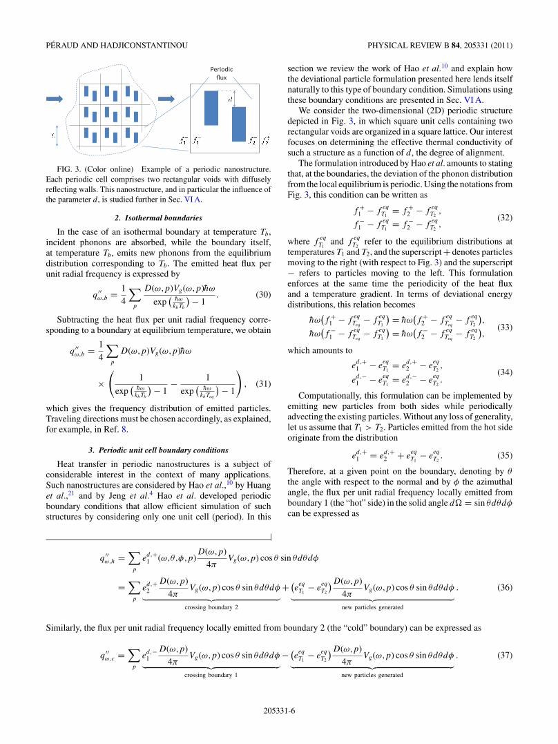
In order to validate the proposed formulation, we firstconsider a one-dimensional system bounded by two isothermal(Sec. III E 2) boundaries that are sufficiently close—theirdistance apart, L, is much smaller than all phonon mean freepaths—that transport can be modeled as ballistic. The systemis initially at a uniform equilibrium temperature T0, when att = 0+ the temperature of the isothermal walls impulsivelychanges to T0 ± T .

Appendix B presents an analytical solution for the resultingtransient evolution of the temperature field that is used herefor comparison with our simulations. A particularly interestingcase is the Debye model which, when coupled with smalltemperature amplitudes, allows a linearization of the generalrelation (B4) to provide a fairly simple closed-form solution(B5). Figure 4 shows a comparison between this solution and

: t=65ps

: t=162.5ps

: t=13ns

FIG. 4. (Color online) Transient temperature profile in a one-dimensional ballistic system whose boundary temperatures undergoan impulsive change at t = 0. Initially, the system is in equilibriumat temperature T0 = 300 K. At t = 0+, the wall temperatures becomeT0 ± T ; here, T = 3 K.

the variance-reduced Monte Carlo result. The simulation wasrun with Teq = T0 and the phonon velocity was taken to be12 360 m s−1.10 Excellent agreement is observed.

B. Heat flux and thermal conductivity in a thin slab

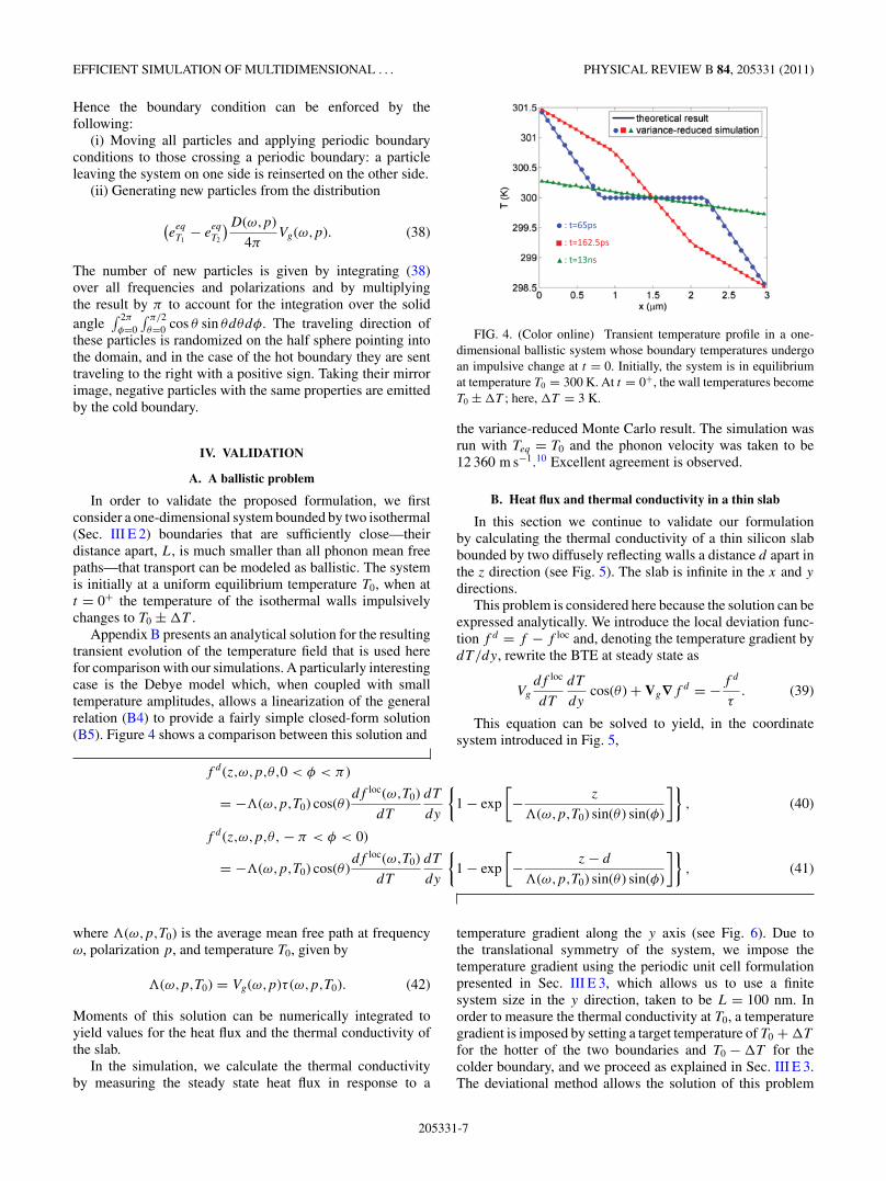
In this section we continue to validate our formulationby calculating the thermal conductivity of a thin silicon slabbounded by two diffusely reflecting walls a distance d apart inthe z direction (see Fig. 5). The slab is infinite in the x and y

directions.This problem is considered here because the solution can be

expressed analytically. We introduce the local deviation func-tion f d = f − f loc and, denoting the temperature gradient bydT /dy, rewrite the BTE at steady state as

Vg

df loc

dT

dT

dycos(θ ) + Vg∇f d = −f d

τ. (39)

This equation can be solved to yield, in the coordinatesystem introduced in Fig. 5,

f d (z,ω,p,θ,0 < φ < π )

= −�(ω,p,T0) cos(θ )df loc(ω,T0)

dT

dT

dy

{1 − exp

[− z

�(ω,p,T0) sin(θ ) sin(φ)

]}, (40)

f d (z,ω,p,θ, − π < φ < 0)

= −�(ω,p,T0) cos(θ )df loc(ω,T0)

dT

dT

dy

{1 − exp

[− z − d

�(ω,p,T0) sin(θ ) sin(φ)

]}, (41)

where �(ω,p,T0) is the average mean free path at frequencyω, polarization p, and temperature T0, given by

�(ω,p,T0) = Vg(ω,p)τ (ω,p,T0). (42)

Moments of this solution can be numerically integrated toyield values for the heat flux and the thermal conductivity ofthe slab.

In the simulation, we calculate the thermal conductivityby measuring the steady state heat flux in response to a

temperature gradient along the y axis (see Fig. 6). Due tothe translational symmetry of the system, we impose thetemperature gradient using the periodic unit cell formulationpresented in Sec. III E 3, which allows us to use a finitesystem size in the y direction, taken to be L = 100 nm. Inorder to measure the thermal conductivity at T0, a temperaturegradient is imposed by setting a target temperature of T0 + T

for the hotter of the two boundaries and T0 − T for thecolder boundary, and we proceed as explained in Sec. III E 3.The deviational method allows the solution of this problem

205331-7

PERAUD AND HADJICONSTANTINOU PHYSICAL REVIEW B 84, 205331 (2011)

Diffuse wall

d

FIG. 5. (Color online) Heat conduction in a silicon slab due toan imposed temperature gradient in the y direction. Slab is infinite inthe x and y directions.

for T � T0 (here, T = 0.05 K), in contrast to non-variance-reduced methods that would require T ∼ T0 toachieve statistically significant results. The best choice forthe equilibrium (control) temperature is clearly Teq = T0 =300 K. Initialization of the simulation at equilibrium at T0 isalso convenient, because no particles need to be generated forthe initial configuration.

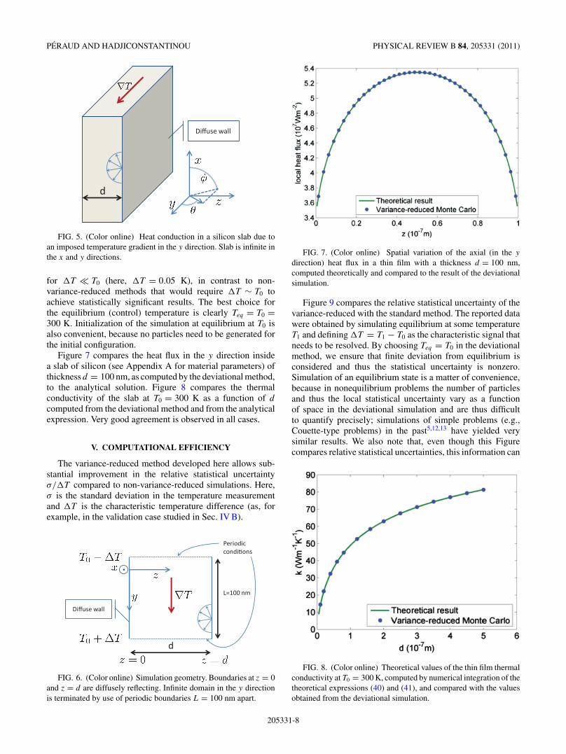
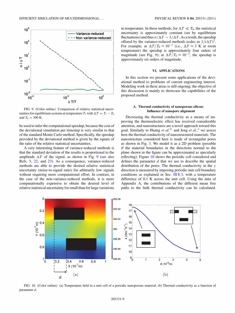
Figure 7 compares the heat flux in the y direction insidea slab of silicon (see Appendix A for material parameters) ofthickness d = 100 nm, as computed by the deviational method,to the analytical solution. Figure 8 compares the thermalconductivity of the slab at T0 = 300 K as a function of d

computed from the deviational method and from the analyticalexpression. Very good agreement is observed in all cases.

V. COMPUTATIONAL EFFICIENCY

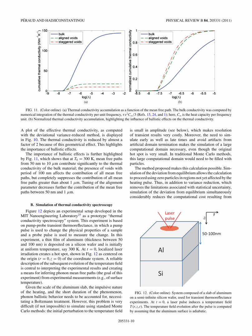
The variance-reduced method developed here allows sub-stantial improvement in the relative statistical uncertaintyσ/T compared to non-variance-reduced simulations. Here,σ is the standard deviation in the temperature measurementand T is the characteristic temperature difference (as, forexample, in the validation case studied in Sec. IV B).

d

Diffuse wall

Periodiccondi�ons

L=100 nm

FIG. 6. (Color online) Simulation geometry. Boundaries at z = 0and z = d are diffusely reflecting. Infinite domain in the y directionis terminated by use of periodic boundaries L = 100 nm apart.

FIG. 7. (Color online) Spatial variation of the axial (in the y

direction) heat flux in a thin film with a thickness d = 100 nm,computed theoretically and compared to the result of the deviationalsimulation.

Figure 9 compares the relative statistical uncertainty of thevariance-reduced with the standard method. The reported datawere obtained by simulating equilibrium at some temperatureT1 and defining T = T1 − T0 as the characteristic signal thatneeds to be resolved. By choosing Teq = T0 in the deviationalmethod, we ensure that finite deviation from equilibrium isconsidered and thus the statistical uncertainty is nonzero.Simulation of an equilibrium state is a matter of convenience,because in nonequilibrium problems the number of particlesand thus the local statistical uncertainty vary as a functionof space in the deviational simulation and are thus difficultto quantify precisely; simulations of simple problems (e.g.,Couette-type problems) in the past5,12,13 have yielded verysimilar results. We also note that, even though this Figurecompares relative statistical uncertainties, this information can

FIG. 8. (Color online) Theoretical values of the thin film thermalconductivity at T0 = 300 K, computed by numerical integration of thetheoretical expressions (40) and (41), and compared with the valuesobtained from the deviational simulation.

205331-8

EFFICIENT SIMULATION OF MULTIDIMENSIONAL . . . PHYSICAL REVIEW B 84, 205331 (2011)

FIG. 9. (Color online) Comparison of relative statistical uncer-tainties for equilibrium systems at temperature T1 with T = T1 − T0

and T0 = 300 K.

be used to infer the computational speedup, because the cost ofthe deviational simulation per timestep is very similar to thatof the standard Monte Carlo method. Specifically, the speedupprovided by the deviational method is given by the square ofthe ratio of the relative statistical uncertainties.

A very interesting feature of variance-reduced methods isthat the standard deviation of the results is proportional to theamplitude T of the signal, as shown in Fig. 9 (see alsoRefs. 5, 22, and 23). As a consequence, variance-reducedmethods are able to provide the desired relative statisticaluncertainty (noise-to-signal ratio) for arbitrarily low signalswithout requiring more computational effort. In contrast, inthe case of the non-variance-reduced methods, it is morecomputationally expensive to obtain the desired level ofrelative statistical uncertainty for small than for large variations

in temperature. In these methods, for T � T0, the statisticaluncertainty is approximately constant (set by equilibriumfluctuations) and thus σ/T ∼ 1/T . As a result, the speedupoffered by the variance-reduced methods scales as 1/(T )2.For example, at T/T0 ≈ 10−2 (i.e., T ≈ 3 K at roomtemperature) the speedup is approximately four orders ofmagnitude (see Fig. 9); at T/T0 ≈ 10−3, the speedup isapproximately six orders of magnitude.

VI. APPLICATIONS

In this section we present some applications of the devi-ational method to problems of current engineering interest.Modeling work in these areas is still ongoing; the objective ofthis discussion is mainly to showcase the capabilities of theproposed method.

A. Thermal conductivity of nanoporous silicon:Influence of nanopore alignment

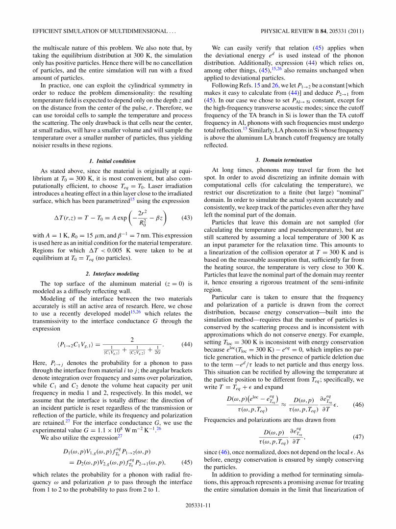
Decreasing the thermal conductivity as a means of im-proving the thermoelectric effect has received considerableattention, and nanostructures are a novel approach toward thisgoal. Similarly to Huang et al.21 and Jeng et al.,4 we assesshere the thermal conductivity of nanostructured materials. Thenanostructure considered here is made of rectangular poresas shown in Fig. 3. We model it as a 2D problem (possibleif the material boundaries in the directions normal to theplane shown in the figure can be approximated as specularlyreflecting). Figure 10 shows the periodic cell considered anddefines the parameter d that we use to describe the spatialdistribution of the pores. The thermal conductivity in the y

direction is measured by imposing periodic unit cell boundaryconditions as explained in Sec. III E 3, with a temperaturedifference of 0.1 K across the unit cell. Using the data ofAppendix A, the contributions of the different mean freepaths to the bulk thermal conductivity can be calculated.

d

FIG. 10. (Color online) (a) Temperature field in a unit cell of a periodic nanoporous material. (b) Thermal conductivity as a function ofparameter d .

205331-9

PERAUD AND HADJICONSTANTINOU PHYSICAL REVIEW B 84, 205331 (2011)

FIG. 11. (Color online) (a) Thermal conductivity accumulation as a function of the mean free path. The bulk conductivity was computed bynumerical integration of the thermal conductivity per unit frequency, τv2Cω/3 (Refs. 15, 24, and 1); here, Cω is the heat capacity per frequencyunit. (b) Normalized thermal conductivity accumulation, highlighting the influence of ballistic effects on the thermal conductivity.

A plot of the effective thermal conductivity, as computedwith the deviational variance-reduced method, is displayedin Fig. 10. The thermal conductivity is reduced by almost afactor of 2 because of this geometrical effect. This highlightsthe importance of ballistic effects.

The importance of ballistic effects is further highlightedby Fig. 11, which shows that at T0 = 300 K, mean free pathsfrom 50 nm to 10 μm contribute significantly to the thermalconductivity of the bulk material; the presence of voids withperiod of 100 nm affects the contribution of all mean freepaths, but completely suppresses the contribution of all meanfree paths greater than about 1 μm. Tuning of the alignmentparameter decreases further the contribution of the mean freepaths between 50 nm and 1 μm.

B. Simulation of thermal conductivity spectroscopy

Figure 12 depicts an experimental setup developed in theMIT Nanoengineering Laboratory25 as a prototype “thermalconductivity spectroscopy” system. This experiment is basedon pump-probe transient thermoreflectance, in which a pumppulse is used to change the physical properties of a sampleand a probe pulse is used to measure the change. In thisexperiment, a thin film of aluminum (thickness between 50and 100 nm) is deposited on a silicon wafer and is initiallyat uniform temperature, say 300 K. At t = 0, localized laserirradiation creates a hot spot, shown in Fig. 12 as centered onthe origin (r = 0,z = 0) of the coordinate system. A reliabledescription of the subsequent evolution of the temperature fieldis central to interpreting the experimental results and creatinga means for inferring phonon mean free paths (the goal of thisexperiment) from experimental measurements (e.g., of surfacetemperature).

Given the scale of the aluminum slab, the impulsive natureof the heating, and the short duration of the phenomenon,phonon ballistic behavior needs to be accounted for, necessi-tating a Boltzmann treatment. However, this problem is verydifficult (if not impossible) to simulate using standard MonteCarlo methods: the initial perturbation to the temperature field

is small in amplitude (see below), which makes resolutionof transient results very costly. Moreover, the need to sim-ulate early as well as late times and avoid artifacts fromartificial domain termination makes the simulation of a largecomputational domain necessary, even though the originalhot spot is very small. In traditional Monte Carlo methods,this large computational domain would need to be filled withparticles.

The method proposed makes this calculation possible. Sim-ulation of the deviation from equilibrium allows the calculationto proceed using zero particles in regions not yet affected by theheating pulse. Thus, in addition to variance reduction, whichremoves the limitations associated with statistical uncertainty,simulation of the deviation from equilibrium simultaneouslyconsiderably reduces the computational cost resulting from

Laser pulse

Al

Si

50-100nm

FIG. 12. (Color online) System composed of a slab of aluminumon a semi-infinite silicon wafer, used for transient thermoreflectanceexperiments. At t = 0, a laser pulse induces a temperature fieldT (r,z,t). The temperature field evolution after the pulse is computedby assuming that the aluminum surface is adiabatic.

205331-10

EFFICIENT SIMULATION OF MULTIDIMENSIONAL . . . PHYSICAL REVIEW B 84, 205331 (2011)

the multiscale nature of this problem. We also note that, bytaking the equilibrium distribution at 300 K, the simulationonly has positive particles. Hence there will be no cancellationof particles, and the entire simulation will run with a fixedamount of particles.

In practice, one can exploit the cylindrical symmetry inorder to reduce the problem dimensionality: the resultingtemperature field is expected to depend only on the depth z andon the distance from the center of the pulse, r . Therefore, wecan use toroidal cells to sample the temperature and processthe scattering. The only drawback is that cells near the center,at small radius, will have a smaller volume and will sample thetemperature over a smaller number of particles, thus yieldingnoisier results in these regions.

1. Initial condition

As stated above, since the material is originally at equi-librium at T0 = 300 K, it is most convenient, but also com-putationally efficient, to choose Teq = T0. Laser irradiationintroduces a heating effect in a thin layer close to the irradiatedsurface, which has been parametrized15 using the expression

T (r,z) = T − T0 = A exp

(−2r2

R20

− βz

)(43)

with A = 1 K, R0 = 15 μm, and β−1 = 7 nm. This expressionis used here as an initial condition for the material temperature.Regions for which T < 0.005 K were taken to be atequilibrium at T0 = Teq (no particles).

2. Interface modeling

The top surface of the aluminum material (z = 0) ismodeled as a diffusely reflecting wall.

Modeling of the interface between the two materialsaccurately is still an active area of research. Here, we choseto use a recently developed model15,26 which relates thetransmissivity to the interface conductance G through theexpression

〈P1→2C1Vg,1〉 = 21

〈C1Vg,1〉 + 1〈C2Vg,2〉 + 1

2G

. (44)

Here, Pi→j denotes the probability for a phonon to passthrough the interface from material i to j ; the angular bracketsdenote integration over frequency and sums over polarization,while C1 and C2 denote the volume heat capacity per unitfrequency in media 1 and 2, respectively. In this model, weassume that the interface is totally diffuse: the direction ofan incident particle is reset regardless of the transmission orreflection of the particle, while its frequency and polarizationare retained.27 For the interface conductance G, we use theexperimental value G = 1.1 × 108 W m−2 K−1.26

We also utilize the expression27

D1(ω,p)V1,g(ω,p)f eq

T0P1→2(ω,p)

= D2(ω,p)V2,g(ω,p)f eq

T0P2→1(ω,p), (45)

which relates the probability for a phonon with radial fre-quency ω and polarization p to pass through the interfacefrom 1 to 2 to the probability to pass from 2 to 1.

We can easily verify that relation (45) applies whenthe deviational energy ed is used instead of the phonondistribution. Additionally, expression (44) which relies on,among other things, (45),15,26 also remains unchanged whenapplied to deviational particles.

Following Refs. 15 and 26, we let P1→2 be a constant [whichmakes it easy to calculate from (44)] and deduce P2→1 from(45). In our case we chose to set PAl→ Si constant, except forthe high-frequency transverse acoustic modes; since the cutofffrequency of the TA branch in Si is lower than the TA cutofffrequency in Al, phonons with such frequencies must undergototal reflection.15 Similarly, LA phonons in Si whose frequencyis above the aluminum LA branch cutoff frequency are totallyreflected.

3. Domain termination

At long times, phonons may travel far from the hotspot. In order to avoid discretizing an infinite domain withcomputational cells (for calculating the temperature), werestrict our discretization to a finite (but large) “nominal”domain. In order to simulate the actual system accurately andconsistently, we keep track of the particles even after they haveleft the nominal part of the domain.

Particles that leave this domain are not sampled (forcalculating the temperature and pseudotemperature), but arestill scattered by assuming a local temperature of 300 K asan input parameter for the relaxation time. This amounts toa linearization of the collision operator at T = 300 K and isbased on the reasonable assumption that, sufficiently far fromthe heating source, the temperature is very close to 300 K.Particles that leave the nominal part of the domain may reenterit, hence ensuring a rigorous treatment of the semi-infiniteregion.

Particular care is taken to ensure that the frequencyand polarization of a particle is drawn from the correctdistribution, because energy conservation—built into thesimulation method—requires that the number of particles isconserved by the scattering process and is inconsistent withapproximations which do not conserve energy. For example,setting Tloc = 300 K is inconsistent with energy conservationbecause eloc(Tloc = 300 K) − eeq = 0, which implies no par-ticle generation, which in the presence of particle deletion dueto the term −ed/τ leads to net particle and thus energy loss.This situation can be rectified by allowing the temperature atthe particle position to be different from Teq ; specifically, wewrite T = Teq + ε and expand

D(ω,p)(eloc − e

eq

Teq

)τ (ω,p,Teq)

≈ D(ω,p)

τ (ω,p,Teq)

∂eeq

Teq

∂Tε. (46)

Frequencies and polarizations are thus drawn from

D(ω,p)

τ (ω,p,Teq)

∂eeq

Teq

∂T, (47)

since (46), once normalized, does not depend on the local ε. Asbefore, energy conservation is ensured by simply conservingthe particles.

In addition to providing a method for terminating simula-tions, this approach represents a promising avenue for treatingthe entire simulation domain in the limit that linearization of

205331-11

PERAUD AND HADJICONSTANTINOU PHYSICAL REVIEW B 84, 205331 (2011)

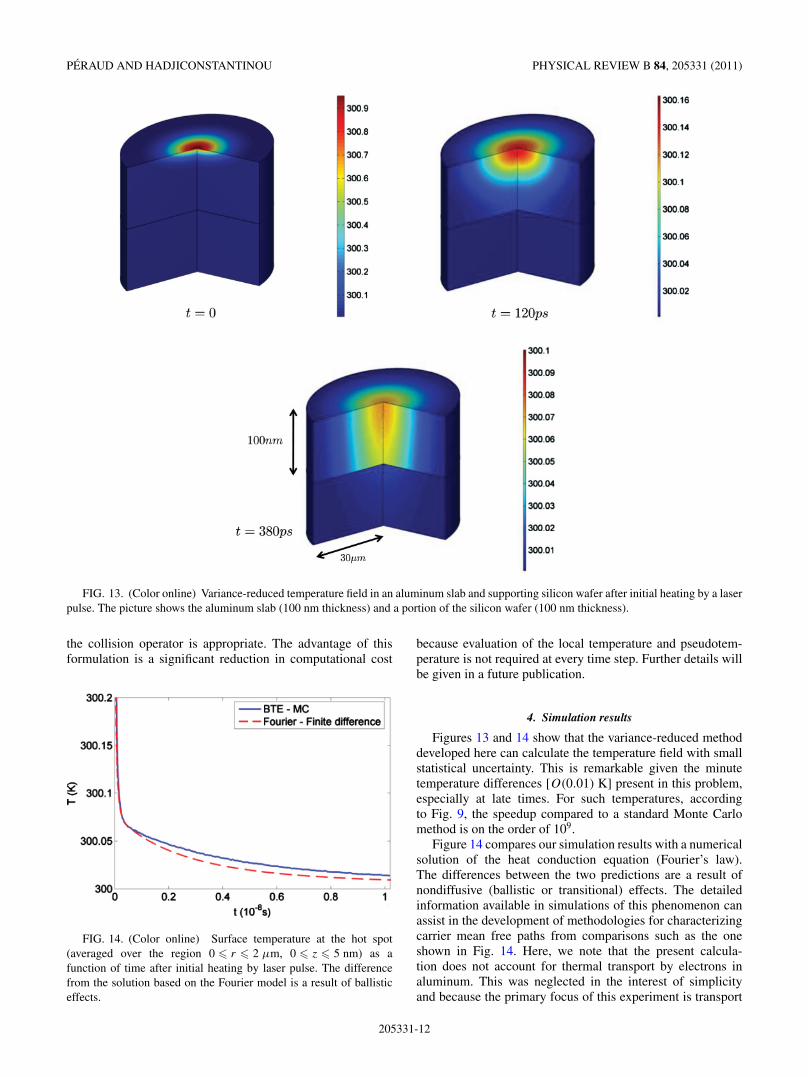
FIG. 13. (Color online) Variance-reduced temperature field in an aluminum slab and supporting silicon wafer after initial heating by a laserpulse. The picture shows the aluminum slab (100 nm thickness) and a portion of the silicon wafer (100 nm thickness).

the collision operator is appropriate. The advantage of thisformulation is a significant reduction in computational cost

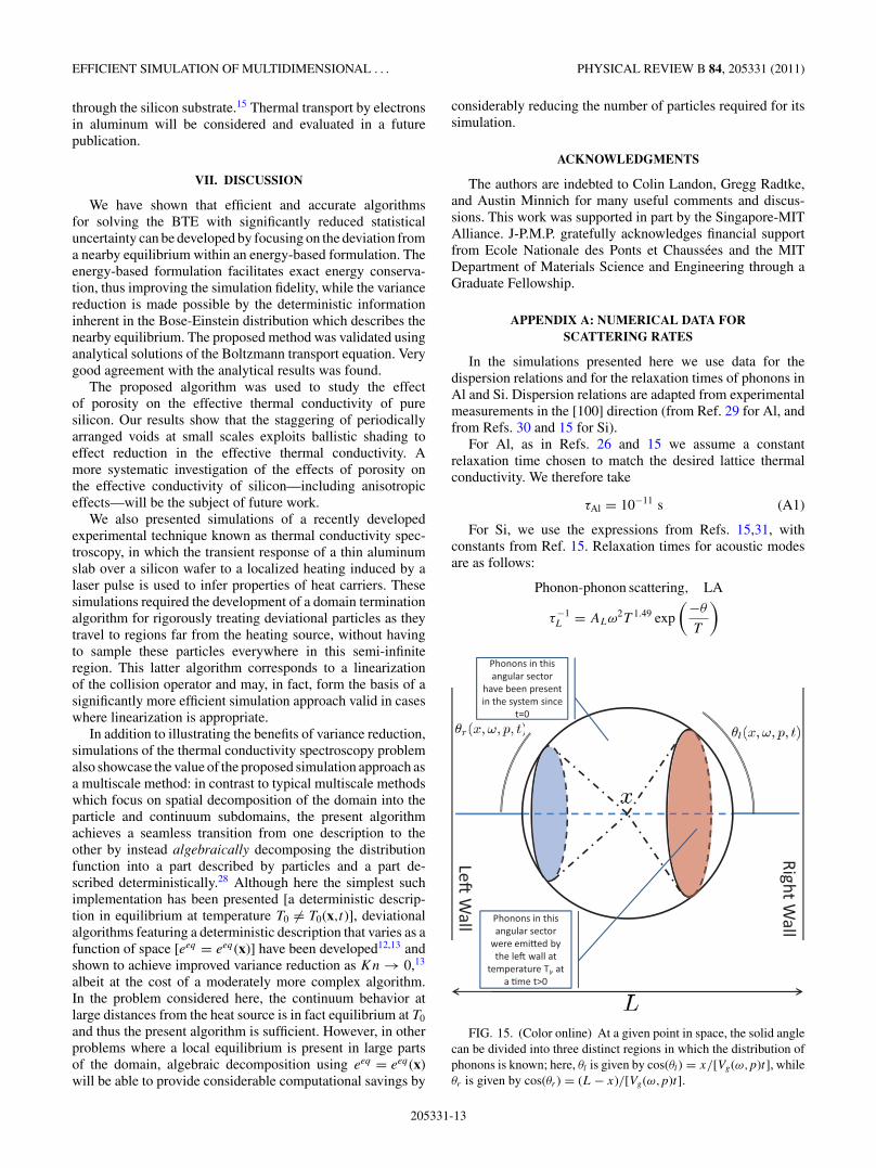
FIG. 14. (Color online) Surface temperature at the hot spot(averaged over the region 0 � r � 2 μm, 0 � z � 5 nm) as afunction of time after initial heating by laser pulse. The differencefrom the solution based on the Fourier model is a result of ballisticeffects.

because evaluation of the local temperature and pseudotem-perature is not required at every time step. Further details willbe given in a future publication.

4. Simulation results

Figures 13 and 14 show that the variance-reduced methoddeveloped here can calculate the temperature field with smallstatistical uncertainty. This is remarkable given the minutetemperature differences [O(0.01) K] present in this problem,especially at late times. For such temperatures, accordingto Fig. 9, the speedup compared to a standard Monte Carlomethod is on the order of 109.

Figure 14 compares our simulation results with a numericalsolution of the heat conduction equation (Fourier’s law).The differences between the two predictions are a result ofnondiffusive (ballistic or transitional) effects. The detailedinformation available in simulations of this phenomenon canassist in the development of methodologies for characterizingcarrier mean free paths from comparisons such as the oneshown in Fig. 14. Here, we note that the present calcula-tion does not account for thermal transport by electrons inaluminum. This was neglected in the interest of simplicityand because the primary focus of this experiment is transport

205331-12

EFFICIENT SIMULATION OF MULTIDIMENSIONAL . . . PHYSICAL REVIEW B 84, 205331 (2011)

through the silicon substrate.15 Thermal transport by electronsin aluminum will be considered and evaluated in a futurepublication.

VII. DISCUSSION

We have shown that efficient and accurate algorithmsfor solving the BTE with significantly reduced statisticaluncertainty can be developed by focusing on the deviation froma nearby equilibrium within an energy-based formulation. Theenergy-based formulation facilitates exact energy conserva-tion, thus improving the simulation fidelity, while the variancereduction is made possible by the deterministic informationinherent in the Bose-Einstein distribution which describes thenearby equilibrium. The proposed method was validated usinganalytical solutions of the Boltzmann transport equation. Verygood agreement with the analytical results was found.

The proposed algorithm was used to study the effectof porosity on the effective thermal conductivity of puresilicon. Our results show that the staggering of periodicallyarranged voids at small scales exploits ballistic shading toeffect reduction in the effective thermal conductivity. Amore systematic investigation of the effects of porosity onthe effective conductivity of silicon—including anisotropiceffects—will be the subject of future work.

We also presented simulations of a recently developedexperimental technique known as thermal conductivity spec-troscopy, in which the transient response of a thin aluminumslab over a silicon wafer to a localized heating induced by alaser pulse is used to infer properties of heat carriers. Thesesimulations required the development of a domain terminationalgorithm for rigorously treating deviational particles as theytravel to regions far from the heating source, without havingto sample these particles everywhere in this semi-infiniteregion. This latter algorithm corresponds to a linearizationof the collision operator and may, in fact, form the basis of asignificantly more efficient simulation approach valid in caseswhere linearization is appropriate.

In addition to illustrating the benefits of variance reduction,simulations of the thermal conductivity spectroscopy problemalso showcase the value of the proposed simulation approach asa multiscale method: in contrast to typical multiscale methodswhich focus on spatial decomposition of the domain into theparticle and continuum subdomains, the present algorithmachieves a seamless transition from one description to theother by instead algebraically decomposing the distributionfunction into a part described by particles and a part de-scribed deterministically.28 Although here the simplest suchimplementation has been presented [a deterministic descrip-tion in equilibrium at temperature T0 �= T0(x,t)], deviationalalgorithms featuring a deterministic description that varies as afunction of space [eeq = eeq (x)] have been developed12,13 andshown to achieve improved variance reduction as Kn → 0,13

albeit at the cost of a moderately more complex algorithm.In the problem considered here, the continuum behavior atlarge distances from the heat source is in fact equilibrium at T0

and thus the present algorithm is sufficient. However, in otherproblems where a local equilibrium is present in large partsof the domain, algebraic decomposition using eeq = eeq(x)will be able to provide considerable computational savings by

considerably reducing the number of particles required for itssimulation.

ACKNOWLEDGMENTS

The authors are indebted to Colin Landon, Gregg Radtke,and Austin Minnich for many useful comments and discus-sions. This work was supported in part by the Singapore-MITAlliance. J-P.M.P. gratefully acknowledges financial supportfrom Ecole Nationale des Ponts et Chaussees and the MITDepartment of Materials Science and Engineering through aGraduate Fellowship.

APPENDIX A: NUMERICAL DATA FORSCATTERING RATES

In the simulations presented here we use data for thedispersion relations and for the relaxation times of phonons inAl and Si. Dispersion relations are adapted from experimentalmeasurements in the [100] direction (from Ref. 29 for Al, andfrom Refs. 30 and 15 for Si).

For Al, as in Refs. 26 and 15 we assume a constantrelaxation time chosen to match the desired lattice thermalconductivity. We therefore take

τAl = 10−11 s (A1)

For Si, we use the expressions from Refs. 15,31, withconstants from Ref. 15. Relaxation times for acoustic modesare as follows:

Phonon-phonon scattering, LA

τ−1L = ALω2T 1.49 exp

(−θ

T

)

Le�W

all

Right Wall

Phonons in thisangular sector

have been presentin the system since

t=0

Phonons in thisangular sector

were emi�ed by the le� wall at

temperature Tl, ata �me t>0

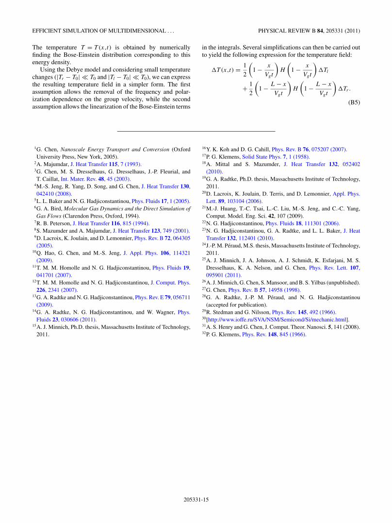
FIG. 15. (Color online) At a given point in space, the solid anglecan be divided into three distinct regions in which the distribution ofphonons is known; here, θl is given by cos(θl) = x/[Vg(ω,p)t], whileθr is given by cos(θr ) = (L − x)/[Vg(ω,p)t].

205331-13

PERAUD AND HADJICONSTANTINOU PHYSICAL REVIEW B 84, 205331 (2011)

Phonon-phonon scattering, TA

τ−1T = AT ω2T 1.65 exp

(−θ

T

)Impurity scattering τ−1

I = AIω4

Boundary scattering τ−1B = wb

where the constants take the following values:

Parameter AL AT θ AI wb

Value (in SI units) 2 × 10−19 1.2 × 10−19 80 3 × 10−45 1.2 × 106

The total relaxation time for a given polarization is obtainedusing the Matthiessen rule

τ−1 =∑

i

τ−1i . (A2)

Optical phonons in Si are considered immobile (Einsteinmodel). Einstein’s model states that the contribution of opticalphonons to the vibrational energy per unit volume in a crystalis given by1

U = NpN ′hωE

V [exp(hωE/kbT ) − 1], (A3)

where Np = 3 is the number of polarizations, N ′ = 1 is thenumber of optical states per lattice point, ωE is the Einstein

radial frequency [ωE = 9.1 × 1013 s−1 (Refs. 30 and 15)], andV is the volume of a lattice point (with a lattice constant a =5.43 A, V = a3/4 = 4 × 10−29 m3).

For the relaxation time of optical phonons, we use thevalue32

τO = 3 × 10−12 s. (A4)

APPENDIX B: DERIVATION OF THE TRANSIENTBALLISTIC 1D SOLUTION

Following the impulsive change of temperature at the wallsfrom T0 to Tl = T0 + T and Tr = T0 − T , thermalizedphonons at temperature Tr and Tl are emitted from the “right”and “left” walls, respectively (see Fig. 15). For some arbitrarylocation x, for a given frequency, polarization, and time,the angular space can be divided into three distinct domainscharacterized by two angles θr (x,ω,p,t) and θl(x,ω,p,t), asdepicted in Fig. 15. Phonons described by 0 < θ < θl wereemitted by the left wall at a time t > 0. Phonons described byθl < θ < π − θr have been present in the system since t = 0.Phonons described by π − θr < θ < π were emitted by theright wall at a time t > 0.

The energy can therefore be written as

EV (x,t) = 1

2

∑p

{∫ω

∫ θl (x,ω,p,t)

θ=0eeq

Tl(ω)D(ω,p) sin(θ )dθdω

+∫

ω

∫ π−θr (x,ω,p,t)

θ=θl (x,ω,p,t)eeq

T0(ω)D(ω,p) sin(θ )dθdω

+∫

ω

∫ π

θ=π−θr (x,ω,p,t)eeq

Tr(ω)D(ω,p) sin(θ )dθdω

}. (B1)

From geometrical considerations,

cos [θr (x,ω,p,t)] = min

(1,

L − x

Vg(ω,p)t

)= 1 −

(1 − L − x

Vg(ω,p)t

)H

(1 − L − x

Vg(ω,p)t

), (B2)

cos [θl(x,ω,p,t)] = min

(1,

x

Vg(ω,p)t

)= 1 −

(1 − x

Vg(ω,p)t

)H

(1 − x

Vg(ω,p)t

), (B3)

where H is the Heaviside function. Proceeding to the integration in θ , the energy density is given by

EV (x,t) = 1

2

∑p

{∫ω

(1 − x

Vg(ω,p)t

)H

(1 − x

Vg(ω,p)t

)eeq

Tl(ω)D(ω,p)dω

+∫

ω

(1 − L − x

Vg(ω,p)t

)H

(1 − L − x

Vg(ω,p)t

)eeq

Tr(ω)D(ω,p)dω

+∫

ω

[1 −

(1 − x

Vg(ω,p)t

)H

(1 − x

Vg(ω,p)t

)]eeq

T0(ω)D(ω,p)dω

+∫

ω

[1 −

(1 − L − x

Vg(ω,p)t

)H

(1 − L − x

Vg(ω,p)t

)]eeq

T0(ω)D(ω,p)dω

}. (B4)

205331-14

EFFICIENT SIMULATION OF MULTIDIMENSIONAL . . . PHYSICAL REVIEW B 84, 205331 (2011)

The temperature T = T (x,t) is obtained by numericallyfinding the Bose-Einstein distribution corresponding to thisenergy density.

Using the Debye model and considering small temperaturechanges (|Tr − T0| � T0 and |Tl − T0| � T0), we can expressthe resulting temperature field in a simpler form. The firstassumption allows the removal of the frequency and polar-ization dependence on the group velocity, while the secondassumption allows the linearization of the Bose-Einstein terms

in the integrals. Several simplifications can then be carried outto yield the following expression for the temperature field:

T (x,t) = 1

2

(1 − x

Vgt

)H

(1 − x

Vgt

)Tl

+ 1

2

(1 − L − x

Vgt

)H

(1 − L − x

Vgt

)Tr.

(B5)

1G. Chen, Nanoscale Energy Transport and Conversion (OxfordUniversity Press, New York, 2005).

2A. Majumdar, J. Heat Transfer 115, 7 (1993).3G. Chen, M. S. Dresselhaus, G. Dresselhaus, J.-P. Fleurial, andT. Caillat, Int. Mater. Rev. 48, 45 (2003).

4M.-S. Jeng, R. Yang, D. Song, and G. Chen, J. Heat Transfer 130,042410 (2008).

5L. L. Baker and N. G. Hadjiconstantinou, Phys. Fluids 17, 1 (2005).6G. A. Bird, Molecular Gas Dynamics and the Direct Simulation ofGas Flows (Clarendon Press, Oxford, 1994).

7R. B. Peterson, J. Heat Transfer 116, 815 (1994).8S. Mazumder and A. Majumdar, J. Heat Transfer 123, 749 (2001).9D. Lacroix, K. Joulain, and D. Lemonnier, Phys. Rev. B 72, 064305(2005).

10Q. Hao, G. Chen, and M.-S. Jeng, J. Appl. Phys. 106, 114321(2009).

11T. M. M. Homolle and N. G. Hadjiconstantinou, Phys. Fluids 19,041701 (2007).

12T. M. M. Homolle and N. G. Hadjiconstantinou, J. Comput. Phys.226, 2341 (2007).

13G. A. Radtke and N. G. Hadjiconstantinou, Phys. Rev. E 79, 056711(2009).

14G. A. Radtke, N. G. Hadjiconstantinou, and W. Wagner, Phys.Fluids 23, 030606 (2011).

15A. J. Minnich, Ph.D. thesis, Massachusetts Institute of Technology,2011.

16Y. K. Koh and D. G. Cahill, Phys. Rev. B 76, 075207 (2007).17P. G. Klemens, Solid State Phys. 7, 1 (1958).18A. Mittal and S. Mazumder, J. Heat Transfer 132, 052402

(2010).19G. A. Radtke, Ph.D. thesis, Massachusetts Institute of Technology,

2011.20D. Lacroix, K. Joulain, D. Terris, and D. Lemonnier, Appl. Phys.

Lett. 89, 103104 (2006).21M.-J. Huang, T.-C. Tsai, L.-C. Liu, M.-S. Jeng, and C.-C. Yang,

Comput. Model. Eng. Sci. 42, 107 (2009).22N. G. Hadjiconstantinou, Phys. Fluids 18, 111301 (2006).23N. G. Hadjiconstantinou, G. A. Radtke, and L. L. Baker, J. Heat

Transfer 132, 112401 (2010).24J.-P. M. Peraud, M.S. thesis, Massachusetts Institute of Technology,

2011.25A. J. Minnich, J. A. Johnson, A. J. Schmidt, K. Esfarjani, M. S.

Dresselhaus, K. A. Nelson, and G. Chen, Phys. Rev. Lett. 107,095901 (2011).

26A. J. Minnich, G. Chen, S. Mansoor, and B. S. Yilbas (unpublished).27G. Chen, Phys. Rev. B 57, 14958 (1998).28G. A. Radtke, J.-P. M. Peraud, and N. G. Hadjiconstantinou

(accepted for publication).29R. Stedman and G. Nilsson, Phys. Rev. 145, 492 (1966).30[http://www.ioffe.ru/SVA/NSM/Semicond/Si/mechanic.html].31A. S. Henry and G. Chen, J. Comput. Theor. Nanosci. 5, 141 (2008).32P. G. Klemens, Phys. Rev. 148, 845 (1966).

205331-15