Embed Size (px)
Citation preview

Efficient state-space modularization for planning theory behavioral and neural signatures
Daniel McNamee Daniel Wolpert Maacuteteacute Lengyel Computational and Biological Learning Lab
Department of Engineering University of Cambridge
Cambridge CB2 1PZ United Kingdom dmcnamee|wolpert|mlengyelengcamacuk
Abstract
Even in state-spaces of modest size planning is plagued by the ldquocurse of dimenshysionalityrdquo This problem is particularly acute in human and animal cognition given the limited capacity of working memory and the time pressures under which planshyning often occurs in the natural environment Hierarchically organized modular representations have long been suggested to underlie the capacity of biological systems12 to efficiently and flexibly plan in complex environments However the principles underlying efficient modularization remain obscure making it difficult to identify its behavioral and neural signatures Here we develop a normative theory of efficient state-space representations which partitions an environment into distinct modules by minimizing the average (information theoretic) description length of planning within the environment thereby optimally trading off the complexity of planning across and within modules We show that such optimal representations provide a unifying account for a diverse range of hitherto unrelated phenomena at multiple levels of behavior and neural representation
1 Introduction
In a large and complex environment such as a city we often need to be able to flexibly plan so that we can reach a wide variety of goal locations from different start locations How might this problem be solved efficiently Model-free decision making strategies3 would either require relearning a policy determining which actions (eg turn right or left) should be chosen in which state (eg locations in the city) each time a new start or goal location is given ndash a very inefficient use of experience resulting in prohibitively slow learning (but see Ref 4) Alternatively the state-space representation used for determining the policy can be augmented with extra dimensions representing the current goal such that effectively multiple policies can be maintained5 or a large ldquolook-up tablerdquo of action sequences connecting any pair of start and goal locations can be represented ndash again leading to inefficient use of experience and potentially excessive representational capacity requirements
In contrast model-based decision-making strategies rely on the ability to simulate future trajectories in the state space and use this in order to flexibly plan in a goal-dependent manner While such strategies are data- and (long term) memory-efficient they are computationally expensive especially in state-spaces for which the corresponding decision tree has a large branching factor and depth6 Endowing state-space representations with a hierarchical structure is an attractive approach to reducing the computational cost of model-based planning7ndash11 and has long been suggested to be a cornerstone of human cognition1 Indeed recent experiments in human decision-making have gleaned evidence for the use and flexible combination of ldquodecision fragmentsrdquo12 while neuroimaging work has identified hierarchical action-value reinforcement learning in humans13 and indicated that
30th Conference on Neural Information Processing Systems (NIPS 2016) Barcelona Spain
dorsolateral prefrontal cortex is involved in the passive clustering of sequentially presented stimuli when transition probabilities obey a ldquocommunityrdquo structure14
Despite such a strong theoretical rationale and empirical evidence for the existence of hierarchical state-space representations the computational principles underpinning their formation and utilization remain obscure In particular previous approaches proposed algorithms in which the optimal state-space decomposition was computed based on the optimal solution in the original (non-hierarchical) representation1516 Thus the resulting state-space partition was designed for a specific (optimal) environment solution rather than the dynamics of the planning algorithm itself and also required a priori knowledge of the optimal solution to the planning problem (which may be difficult to obtain in general and renders the resulting hierarchy obsolete) Here we compute a hierarchical modularization optimized for planning directly from the transition structure of the environment without assuming any a priori knowledge of optimal behavior Our approach is based on minimizing the average information theoretic description length of planning trajectories in an environment thus explicitly optimizing representations for minimal working memory requirements The resulting representation are hierarchically modular such that planning can first operate at a global level across modules acquiring a high-level ldquorough picturerdquo of the trajectory to the goal and subsequently locally within each module to ldquofill in the detailsrdquo
The structure of the paper is as follows We first describe the mathematical framework for optimizing modular state-space representations (Section 2) and also develop an efficient coding-based approach to neural representations of modularised state spaces (Section 26) We then test some of the key predictions of the theory in human behavioral and neural data (Section 3) and also describe how this framework can explain several temporal and representational characteristics of ldquotask-bracketingrdquo and motor chunking in rodent electrophysiology (Section 4) We end by discussing future extensions and applications of the theory (Section 5)
2 Theory
21 Basic definitions
In order to focus on situations which require flexible policy development based on dynamic goal requirements we primarily consider discrete ldquomultiple-goalrdquo Markov decision processes (MDPs) Such an MDP M = S A T G is composed of a set of states S a set of actions A (a subset As of which is associated with each state s 2 S) and transition function T which determines the probability of transitioning to state sj upon executing action a in state si p(sj |si a) = T (si a sj ) A task (s g) is defined by a start state s 2 S and a goal state g 2 G and the agentrsquos objective is to identify a trajectory of via states v which gets the agent from s to g We define a modularization
1
M of the state-space S to be a set of Boolean matrices M = Mii=1m indicating the module membership of all states s 2 S That is for all s 2 S there exists i 2 1 m such that Mi(s) = 1 Mj (s) = 0 8j =6 i We assume this to form a disjoint cover of the state-space (overlapping modular architectures will be explored in future work) We will abuse notation by using the expression s 2 M to indicate that a state s is a member of a module M As our planning algorithm P we consider random search as a worst-case scenario although in principle our approach applies to any algorithm such as dynamic programming or Q-learning3 and we expect the optimal modularization to depend on the specific algorithm utilized
We describe and analyze planning as a Markov process For planning the underlying state-space is the same as that of the MDP and the transition matrix T is a marginalization over a planning policy
1plan (which here we assume is the random policy rand(a|si) = | )|Asi
Tij =X
plan(a|si) T (si a sj ) (1) a
Given a modularization M planning at the global level is a Markov process MG corresponding to a ldquolow-resolutionrdquo representation of planning in the underlying MDP where each state corresponds
1This is an example of a ldquopropositional representationrdquo 1718 and is analogous to state aggregation or ldquoclusshyteringrdquo 1920 in reinforcement learning which is typically accomplished via heuristic bottleneck discovery algoshyrithms 21 Our method is novel in that it does not require the optimal policy as an input and is founded on a normative principle
2
to a ldquolocalrdquo module Mi and the transition structure TG is induced from T via marginalization and normalization22 over the internal states of the local modules Mi
22 Description length of planning
We use an information-theoretic framework2324 to define a measure the (expected) description length (DL) of planning which can be used to quantify the complexity of planning P in the induced global L(P|MG) and local modules L(P|Mi) We will compute the DL of planning L(P) in a non-modularized setting and outline the extension to modularized planning DL L(P|M) (elaborating further in the supplementary material) Given a task (s g) in an MDP a solution v(n) to this task
(n) (n)is an n-state trajectory such that v = s and vn = g The description length (DL) of this 1
trajectory is L(v(n)) = - log pplan(v(n)) A task may admit many solutions corresponding to different trajectories over the state-space thus we define the DL of the task (s g) to be the expectation over all trajectories which solve this task namely
1
L(s g) = Evn
hL(v(n))
i = -
X X p(v(n)|s g) log p(v(n)|s g) (2)
n=1 v(n)
This is the (s g)-th entry of the trajectory entropy matrix H of M Remarkably this can be expressed in closed form25
[H]sg = X
[(I - Tg )-1]sv Hv (3)
v 6=g
where T is the transition matrix of the planning Markov chain (Eq 1) Tg is a sub-matrix correspondshying to the elimination of the g-th column and row and Hv is the local entropy Hv = H(Tvmiddot) at state v Finally we define the description length L(P) of the planning process P itself over all tasks (s g)
L(P) = Esg [L(s g)] = X
Ps Pg L(s g) (4) (sg)
where Ps and Pg are priors of the start and goal states respectively which we assume to be factorizable P(sg) = Ps Pg for clarity of exposition In matrix notation this can be expressed as L(P) = Ps H Pg
T
where Ps is a row-vector of start state probabilities and Pg is a row-vector of goal state probabilities
The planning DL L(P|M) of a nontrivial modularization of an MDP requires (1) the computation of the DL of the global L(P|MG) and the local planning processes L(P|Mi) for global MG and local Mi modular structures respectively and (2) the weighting of these quantities by the correct priors See supplementary material for further details
23 Minimum modularized description length of planning
Based on a modularization planning can be first performed at the global level across modules and then subsequently locally within the subset of modules identified by the global planning process (Fig 1) Given a task (s g) where s represents the start state and g represents the goal state global search would involve finding a trajectory in MG from the induced initial module (the unique Ms such that Ms(s) = 1) to the goal module (Mg (g) = 1) The result of this search will be a global directive across modules Ms middot middot middot Mg Subsequently local planning sub-tasks are solved within each module in order to ldquofill in the detailsrdquo For each module transition Mi Mj in MG a local search in Mi is accomplished by planning from an entrance state from the previous module and planning until an exit state for module Mj is entered This algorithm is illustrated in Figure 1
By minimizing the sum of the global L(P|MG) and local DLs L(P|Mi) we establish the optimal modularization M of a state-space for planning
M = arg min [L(P|M) + L(M)] where L(P|M) = L(P|MG) +X
L(P|Mi) (5)M
i
Note that this formulation explicitly trades-off the complexity (measured as DL) of planning at the global level L(P|MG) ie across modules and at the local level L(P|Mi) ie within individual modules (Fig 1C-D) In principle the representational cost of the modularization itself L(M) is also
3
Pla
nnin
gde
scrip
tion
leng
th(n
ats)
Fig 1 ldquoExplanationrdquo
0 1 2 3
Entropic centrality (bits)times104
1
2
3
4
5
6
De
gre
e c
en
tra
lity
(co
nn
ect
ed
sta
tes)
05 1 15 2 25 3Compression Factor
0
005
01
015
02
025
Prob
abilit
y
-1 0 1 2
Within- vs Across-Module
-50
0
50
100
Rank
Sum
Sco
re (
larg
er
=gt
more
sim
ilar)
-1 0 1 2
Within- vs Across-Module
0
2000
4000
6000
EC
Eucl
idean D
ista
nce
Normalized Euclidean dist between EC ordered by module
0
05
1
Modules
-1 0 1 2
Within- vs Across-Module
-50
0
50
Ra
nk
Su
m S
core
(la
rge
r =
gt m
ore
sim
ilar)
-1 0 1 2
Within- vs Across-Module
0
2000
4000
6000
Ab
solu
te d
iffe
ren
ce in
EC
Normalized Euclidean dist between EC ordered by module
0
05
1
Modules
Soho Modularization
L(P|M)
X
i
L(P|Mi)
L(P|MG)
Modularized Soho Trajectories
Module
s
Across
Module
s
part of the trade-off but we do not consider it further here for two reasons First in the state-spaces considered in this paper it is dwarfed by the the complexities of planning L(M) L(P|M) (see the supplementary material for the mathematical characterization of L(M)) Second it taxes long-term rather than short-term memory which is at a premium when planning2627 Importantly although computing the DL of a modularization seems to pose significant computational challenges by requiring the enumeration of a large number of potential trajectories in the environment (across or within modules) in the supplementary material we show that it can be computed in a relatively straightforward manner (the only nontrivial operation being a matrix inversion) using the theory of finite Markov chains22
24 Planning compression
The planning DL L(s g) for a specific task (s g) describes the expected difficulty in finding an intervening trajectory v for a task (s g) For example in a binary coding scheme where we assign binary sequences to each state the expected length of string of random 0s and 1s corresponding to a trajectory will be shorter in a modularized compared to a non-modularized representation Thus we can examine the relative benefit of an optimal modularization in the Shannon limit by computing the ratio of trajectory description lengths in modularized and non-modularized representations of a task or environment28 In line with spatial cognition terminology29 we refer to this ratio as the compression factor of the trajectory
A BFlat Planning Modularized Planning Global Local
M1 M2 M3
middot middot middots1 g1 middot middot middots2 g2 middot middot middots3 g3
Global
Local
G
SS
G
S
G
SG
S
G
S
G
L(P|MG)Planning Entropy
L(P|M1) L(P|M2) L(P|M3)XL(P) L(P|MG) L(P|Mi) Time
i
C D E F G 6Londonrsquos Soho Optimizing Modularization
25
2
15
1
05
0 EC
Euc
lidea
n D
ista
nce
(kna
ts)
N 50m
6
Frac
tion
5
4
3
2
Deg
ree
cent
ralit
y
With
in
4
2
10 0 1 2 35 1 15 2 25 3 Entropic centrality (knats)Number of modules Soho trajectory compression factor
Figure 1 Modularized planning A Schematic exhibiting how planning which could be highly complex using a flat state space representation (left) can be reformulated into a hierarchical planning process via a modularization (center and right) Boxes (circles or squares) show states lines are transitions (gray potential transitions black transitions considered in current plan) Once the ldquoglobal directiverdquo has been established by searching in a low-resolution representation of the environment (center) the agent can then proceed to ldquofill in the detailsrdquo by solving a series of local planning sub-tasks (right) Formulae along the bottom show the DL of the corresponding planning processes B Given a modularization a serial hierarchical planning process unfolds in time beginning with a global search task followed by local sub-tasks As each globallocal planning task is initiated in series there is a phasic increase in processing which scales with planning difficulty in the upcoming module as quantified by the local DL L(P|Mi) C Map of Londonrsquos Soho state-space streets (lines with colors coding degree centrality) correspond to states (courtesy of Hugo Spiers) D Minimum expected planning DL of Londonrsquos Soho as a function of the number of modules (minimizing over all modularizations with the given number of modules) Red global blue local black total DL E Histogram of compression factors of 200 simulated trajectories from randomly chosen start to goal locations in Londonrsquos Soho F Absolute entropic centrality (EC) differences within and across connected modules in the optimal modularization of the Soho state-space G Scatter plot of degree and entropic centralities of all states in the Soho state-space
4
25 Entropic centrality
The computation of the planning DL (Section 22) makes use of the trajectory entropy matrix H of a Markov chain Since H is composed of weighted sums of local entropies Hv it suggests that we can express the contribution of a particular state v to the planning DL by summing its terms for all tasks (s g) Thus we define the entropic centrality Ev of a state v via
Ev = X
Dsvg Hv (6) sg
where we have made use of the fundamental tensor of a Markov chain D with components Dsvg = (I - Tg)-1
Note that task priors can easily be incorporated into this definition The entropic
svcentrality (EC) of a state measures its importance to tasks across the domain and its gradient can serve as a measure of ldquosubgoalnessrdquo for the planning process P Indeed we observed in simulations that one strategy used by an optimal modularization to minimize planning complexity is to ldquoisolaterdquo planning DL within rather than across modules such that EC changes more across than within modules (Fig 1F) This suggests that changes in EC serve as a good heuristic for identifying modules
Furthermore EC is tightly related to the graph-theoretic notion of degree centrality (DC) When transhysitions are undirected and are deterministically related to action degree centrality deg(v) corresponds to the number of states which are accessible from a state v In such circumstances and assuming a random policy we have
1 Ev =
X Dsvg log(deg(v)) (7)
deg(v)sg
The ECs and DCs of all states in a state-space reflecting the topology of Londonrsquos Soho are plotted in Fig 1G and show a strong correlation in agreement with this analysis In Section 32 we test whether this tight relationship together with the intuition developed above about changes in EC demarcating approximate module boundaries provides a normative account of recently observed correlations between DC and human hippocampal activity during spatial navigation30
26 Efficient coding in modularized state-spaces
In addition to ldquocompressingrdquo the planning process modularization also enables a neural channel to transmit information (for example a desired state sequence) in a more efficient pattern of activity using a hierarchical entropy coding strategy31 whereby contextual codewords signaling the entrance to and exit from a module constrain the set of states that can be transmitted to those within a module thus allowing them to be encoded with shorter description lengths according to their relative probabilities28 (ie a state that forms part of many trajectory will have a shorter description length than one that does not) Assuming that neurons take advantage of these strategies in an efficient code32 several predictions can be made with regard to the representational characteristics of neuronal populations encoding components of optimally modularized state-spaces We suggest that the phasic neural responses (known as ldquostartrdquo and ldquostoprdquo signals) which have been observed to encase learned behavioral sequences in a wide range of control paradigms across multiple species33ndash36 serve this purpose in modularized control architectures Our theory makes several predictions regarding the temporal dynamics and population characteristics of these startstop codes First it determines a specific temporal pattern of phasic startstop activity as an animal navigates using an optimally modularized representation of a state-space Second neural representations for the start signals should depend on the distribution of modules while the stop codes should be sensitive to the distribution of components within a module Considering the minimum average description length of each of these distribution we can make predictions regarding how much neural resources (for example the number of neurons) should be assigned to represent each of these startstop variables We verify these predictions in published neural data3634 in Section 4
3 Route compression and state-space segmentation in spatial cognition
31 Route compression
We compared the compression afforded by optimal modularization to a recent behavioral study examining trajectory compression during mental navigation29 In this task students at the University
5
Fig 2 ldquoSpatialCogrdquo
Route length (states)0 2 4 6 8 10
Com
pres
sion
09
1
11
12
13
14
15
16
17Modularized Soho Simulations
R2 = 046R2 = 072
Route length (m)0 200 400 600 800 1000
Com
pres
sion
0
5
10
15
20
25
30
35
40Empirical Data (Bonasia et al 2016)
R2 = 069R2 = 082
Com
pres
sion
Empirical Data (Bonasia et al 2016)
Com
pres
sion
Modularized Soho Simulations
of Toronto were asked to mentally navigate between a variety of start and goal locations on their campus and the authors computed the (inverse) ratio between the duration of this mental navigation and the typical time it would physically take to walk the same distance Although mental navigation time was substantially smaller than physical time it was not simply a constant fraction of it but instead the ratio of the two (the compression factor) became higher with longer route length (Fig 2A) In fact while in the original study only a linear relationship between compression factor and physical route length was considered reanalysing the data yielded a better fit by a logarithmic function (R2 = 069 vs 046)
In order to compare our theory with these data we computed compression factors between the optimally modularized and the non-modularized version of an environment This was because students were likely to have developed a good knowledge of the campusrsquo spatial structure and so we assumed they used an approximately optimal modularization for mental navigation while the physical walking time could not make use of this modularization and was bound to the original non-modularized topology of the campus As we did not have access to precise geographical data about the part of the U Toronto campus that was used in the original experiment we ran our algorithm on a part of London Soho which had been used in previous studies of human navigation30 Based on 200 simulated trajectories over route lengths of 1 to 10 states we found that our compression factor showed a similar dependence on route length2 (Fig 2B) and again was better fit by a logarithmic versus a linear function (R2 = 082 vs 072 respectively)
A Human Navigated Trajectories B Simulated Modularized Trajectories C L(P|Mi) vs Centrality Correlations
Com
pres
sion
fact
or
40
35
30
25
20
15
10
5
00 200 400 600 800 1000
R2 = 069 R2 = 082
0 2 4 6 8 1009
1
11
12
13
14
15
16
17
R2 = 046 R2 = 072
Com
pres
sion
fact
or
Degree Between Closeness
1
08
06
04
02
0
Route length (m) Route length (states)
Figure 2 Modularized representations for spatial cognition A Compression factor as a function of route length for navigating the U Toronto campus (reproduced from Ref 29) with linear (grey) and logarithmic fits (blue) B Compression factors for the optimal modularization in the London Soho environment C Spearman correlations between changes in local planning DL L(P|Mi) and changes in different graph-theoretic measures of centrality
32 Local planning entropy and degree centrality
We also modeled a task in which participants who were trained to be familiar with the environment navigated between randomly chosen locations in a virtual reality representation of Londonrsquos Soho by pressing keys to move through the scenes30 Functional magnetic resonance imaging during this task showed that hippocampal activity during such self-planned (but not guided) navigation correlated most strongly with changes in a topological state ldquoconnectednessrdquo measure known as degree centrality (DC compared to other standard graph-theoretic measures of centrality such as ldquobetweennessrdquo and ldquoclosenessrdquo) Although changes in DC are not directly relevant to our theory we can show that they serve as a good proxy for a fundamental quantity in the theory planning DL (see Eq 7) which in turn should be reflected in neural activations
To relate the optimal modularization the most direct prediction of our theory to neural signals we made the following assumptions (see also Fig 1B) 1 Planning (and associated neural activity) occurs upon entering a new module (as once a plan is prepared movement across the module can be automatic without the need for further planning until transitioning to a new module) 2 The magnitude of neural activity is related to the local planning DL L(P|Mi) of the module (as the higher the entropy the more trajectories need to be considered likely activating more neurons with different tunings for state transitions or state-action combinations37 resulting in higher overall
2Note that the absolute scale of our compression factor is different from that found in the experiment because we did not account for the trivial compression that comes from the simple fact that it is just generally faster to move mentally than physically
6
Fig 3 ldquoStartstoprdquo
0 05 1 150
5
10
15
0 05 1 150
5
10
15
0 05 1 150
0 05 1 150
Turn S
tart
TurGoa
l
Arrival
Tur TurGoa
l
Arrival
First
Final
Desc
riptio
n le
ngth
(nat
s)
A T-Maze Task Simulated ldquoTask-Responsiverdquo Neurons B C 15
Gate Start
Cue
n End
10
15
Gate Start
Cue
n Star
tn E
nd
Firin
g Ra
te (H
z)
Start
Cue
Turn S
tart
Turn E
ndGoa
l
ArrivalGate
Empirical Data Overtrained Before Acquisition Modularization Overtrained (Modularized)
Firin
g Ra
te (H
z)
Firin
g R
ate
(Hz)
10
5 5
LEFT LEVER
EXPLORE
RIGHT LEVER
MAG ENTRY
LICKFREEZE
GROOM
REST
MAG ENTRY
LICK
LEFT LEVER
RIGHT LEVER
LEFT LEVER
RIGHT LEVER
R
D
Perc
enta
ge
E F
3
2
1
START STOP SEQUENCE SEQUENCE
Figure 3 Neural activities encoding module boundaries A T-maze task in which tone determines the location of the reward (reproduced from Ref 34) Inset the modelrsquos optimal modularization of the discretized T-maze state-space Note that the critical junction has been extracted to form its own module which isolates the local planning DL caused by the split in the path B Empirical data exhibiting the temporal pattern of task-bracketing in dorsolateral striatal (DLS) neurons Prior to learning the task ensemble activity was highly variable both spatially and temporally throughout the behavioral trajectory Reproduced from Ref 34 C Simulated firing rates of ldquotask-responsiverdquo neurons after and before acquiring an optimal modularization D The optimal modularization (colored states are in the same module) of a proposed state-space for an operant conditioning task36 Note that the lever pressing sequences form their own modules and thus require specialized startstop codes E Analyses of striatal neurons suggesting that a larger percentage of neurons encoded lever sequence initiations compared to terminations and that very few encoded both Reproduced from Ref 36 F Description lengths of startstop codes in the optimal modularization
activity in the population) Furthermore as before we also assume that participants were sufficiently familiar with Soho that they used the optimal modularization (as they were specifically trained in the experiment) Having established that under the optimal modularization entropic centrality (EC) tends to change more across than within modules (Fig 1F) and also that EC is closely related to DC (Fig 1G) the theory predicts that neural activity should be timed to changes in DC Furthermore the DLs of successive modules along a trajectory will in general be positively correlated with the differences between their DLs (due to the unavoidable ldquoregression to the meanrdquo effect3) Noting that the planning DL of a module is just the (weighted) average EC of its states (see Section 25) the theory thus more specifically predicts a positive correlation between neural activity (representing the DLs of modules) and changes in EC and therefore changes in DC ndash just as seen in experiments
We verified these predictions numerically by quantifying the correlation of changes in each centrality measure used in the experiments with transient changes in local planning complexity as computed in the model (Fig 2C) Across simulated trajectories we found that changes in DC had a strong correlation with changes in local planning entropy (mean deg = 079) that was significantly higher (p lt 10-5 paired t-tests) than the correlation with the other centrality measures We predict that even higher correlations with neural activity could be achieved if planning DL according to the optimal modularization rather than DC was used directly as a regressor in general linear models of the fMRI data
3Transitioning to a module with largersmaller DL will cause on average a more positivenegative DL change compared to the previous module DL
7
4 Task-bracketing and startstop signals in striatal circuits
Several studies have examined sequential action selection paradigms and identified specialized taskshybracketing3334 and ldquostartrdquo and ldquostoprdquo neurons that are invariant to a wide range of motivational kinematic and environmental variables 3635 Here we show that task-bracketing and startstop signals arise naturally from our model framework in two well-studied tasks one involving their temporal34
and the other their representational characteristics36
In the first study as rodents learned to navigate a T-maze (Fig 3A) neural activity in dorsolateral striatum and infralimbic cortex became increasingly crystallized into temporal patterns known as ldquotask-bracketsrdquo34 For example although neural activity was highly variable before learning after learning the same neurons phasically fired at the start of a behavioral sequence as the rodent turned into and out of the critical junction and finally at the final goal position where reward was obtained Based on the optimal modularization for the T-maze state-space (Fig 3A inset) we examined spike trains from a simulated neurons whose firing rates scaled with local planning entropy (see supplementary material) and this showed that initially (ie without modularization Fig 3C right) the firing rate did not reflect any task-bracketing but following training (ie optimal modularization Fig 3C left) the activity exhibited clear task-bracketing driven by the initiation or completion of a local planning process These result show a good qualitative match to the empirical data (Fig 3B from Ref 34) showing that task-bracketing patterns of activity can be explained as the result of module startstop signaling and planning according to an optimal modular decomposition of the environment
In the second study rodents engaged in an operant conditioning paradigm in which a sequence of eight presses on a left or right lever led to the delivery of high or low rewards36 After learning recordings from nigrostriatal circuits showed that some neurons encoded the initiation and fewer appeared to encode the termination of these action sequences We used our framework to compute the optimal modularization based on an approximation to the task state-space (Fig 3D) in which the rodent could be in many natural behavioral states (red circles) prior to the start of the task Our model found that the lever action sequences were extracted into two separate modules (blue and green circles) Given a modularization a hierarchical entropy coding strategy uses distinct neural codewords for the initiation and termination of each module (Section 26) Importantly we found that the description lengths of start codes was longer than that of stop codes (Fig 3F) Thus an efficient allocation of neural resources predicts more neurons encoding start than stop signals as seen in the empirical data (Fig 3E) Intuitively more bits are required to encode starts than stops in this state-space due to the relatively high level of entropic centrality of the ldquorestrdquo state (where many different behaviors may be initiated red circles) compared to the final lever press state (which is only accessible from the previous Lever press state and where the rodent can only choose to enter the magazine or return to ldquorestrdquo) These results show that the start and stop codes and their representational characteristics arise naturally from an efficient representation of the optimally modularized state space
5 Discussion
We have developed the first framework in which it is possible to derive state-space modularizations that are directly optimized for the efficiency of decision making strategies and do not require prior knowledge of the optimal policy before computing the modularization Furthermore we have identified experimental hallmarks of the resulting modularizations thereby unifying a range of seemingly disparate results from behavioral and neurophysiological studies within a common principled framework An interesting future direction would be to study how modularized policy production may be realized in neural circuits In such cases once a representation has been established neural dynamics at each level of the hierarchy may be used to move along a state-space trajectory via a sequence of attractors with neural adaptation preventing backflow38 or by using fundamentally non-normal dynamics around a single attractor state39 The description length that lies at the heart of the modularization we derived was based on a specific planning algorithm random search which may not lead to the modularization that would be optimal for other more powerful and realistic planning algorithms Nevertheless in principle our approach is general in that it can take any planning algorithm as the component that generates description lengths including hybrid algorithms that combine model-based and model-free techniques that likely underlie animal and human decision making40
8
References 1 Lashley K In Jeffress LA editor Cerebral Mechanisms in Behavior New York Wiley pp 112ndash147 1951 2 Simon H Newell A Human Problem Solving Longman Higher Education 1971 3 Sutton R Barto A Reinforcement Learning An Introduction MIT Press 1998 4 Stachenfeld K et al Advances in Neural Information Processing Systems 2014 5 Moore AW et al IJCAI International Joint Conference on Artificial Intelligence 21318ndash1321 1999 6 Lengyel M Dayan P Advances in Neural Information Processing Systems 2007 7 Dayan P Hinton G Advances in Neural Information Processing Systems 1992 8 Parr R Russell S Advances in Neural Information Processing Systems 1997 9 Sutton R et al Artificial Intelligence 112181 ndash 211 1999
10 Hauskrecht M et al In Uncertainty in Artificial Intelligence 1998 11 Rothkopf CA Ballard DH Frontiers in Psychology 11ndash13 2010 12 Huys QJM et al Proceedings of the National Academy of Sciences 1123098ndash3103 2015 13 Gershman SJ et al Journal of Neuroscience 2913524ndash31 2009 14 Schapiro AC et al Nature Neuroscience 16486ndash492 2013 15 Foster D Dayan P Machine Learning pp 325ndash346 2002 16 Solway A et al PLoS Computational Biology 10e1003779 2014 17 Littman ML et al Journal of Artificial Intelligence Research 91ndash36 1998 18 Boutilier C et al Journal of Artificial Intelligence Research 111ndash94 1999 19 Singh SP et al Advances in Neural Information Processing Systems 1995 20 Kim KE Dean T Artificial Intelligence 147225ndash251 2003 21 Simsek O Barto AG Advances in Neural Information Processing Systems 2008 22 Kemeny JG Snell JL Finite Markov Chains Springer-Verlag 1983 23 Balasubramanian V Neural Computation 9349ndash368 1996 24 Rissanen J Information and Complexity in Statistical Modeling Springer 2007 25 Kafsi M et al IEEE Transactions on Information Theory 595577ndash5583 2013 26 Todd M et al Advances in Neural Information Processing Systems 2008 27 Otto AR et al Psychological Science 24751ndash61 2013 28 MacKay D Information Theory Inference and Learning Algorithms Cambridge University Press 2003 29 Bonasia K et al Hippocampus 269ndash12 2016 30 Javadi AH et al Nature Communications in press 2016 31 Rosvall M Bergstrom CT Proceedings of the National Academy of Sciences 1051118ndash1123 2008 32 Ganguli D Simoncelli E Neural Computation 262103ndash2134 2014 33 Barnes TD et al Nature 4371158ndash61 2005 34 Smith KS Graybiel AM Neuron 79361ndash374 2013 35 Fujii N Graybiel AM Science 3011246ndash1249 2003 36 Jin X Costa RM Nature 466457ndash462 2010 37 Stalnaker TA et al Frontiers in Integrative Neuroscience 412 2010 38 Russo E et al New Journal of Physics 10 2008 39 Hennequin G et al Neuron 821394ndash406 2014 40 Daw ND et al Nature Neuroscience 81704ndash11 2005
9
Supplementary Material for NIPS 2016 Paper 2245 Efficient state-space modularization for planning
theory behavioral and neural signatures
Contents
1 Modularized description length of planning 1
2 Module transition probabilities 2
21 Across-modules transitions and sub-start probabilities 3
22 Within-modules transitions and sub-goal probabilities 3
3 Alternate formulation of trajectory entropy 3
4 Representational cost of modularization 3
5 Experimental datasets and analysis details 4
51 Spatial navigation task 4
52 Task-bracketing simulations 4
53 Operant conditioning state-space 4
6 Comparison with other measures of planning complexitydifficulty 5
7 Comparing efficient modularizations and optimal behavioral hierarchies 5
8 Entropic centrality and state-space bottlenecks 6
1 Modularized description length of planning
The global planning DL L(P|MG) can be easily computed after marginalizing over the inshyternal states of each module Defining PS (PG) to be the prior over start (goal) modules
PS(Mi) = P
s2Mi Ps
PG(Mi) =
P g2Mi
Pg
then L(P|MG) = PS HG PG
T where HG is
the trajectory entropy across modules In order to compute the local planning DL L(P|Mi) = (PS(Mi) + PV(Mi) + PG(Mi))
P sigi2Mi
Psi Pgi L(si gi|Mi) we must first establish the induced priors over ldquosub-tasksrdquo (si gi) within the module Mi The probability that a state si 2 Mi serves as a sub-start state is the probability that si is the entrance state to Mi given a module transition into Mi at the global level Conversely a state gi 2 Mi is a sub-goal state if it is the last transient state within Mi before a trajectory transitions out of the module Mi These probabilities as well as
30th Conference on Neural Information Processing Systems (NIPS 2016) Barcelona Spain
Compression Factor (Huffman Coding)
Prob
abilit
y
Fig 2 ldquoExamplesrdquo
MDP1
WalksTrajectories
MDP 2
Flat Representation Modularization Compression Factors
0
005
01
015
02
025
03
Frac
tion
Random walks State-goal trajectories
06 08 1 12 14 16
03
025
02
015
01
005
0 06 08 1 12 14 16
Compression Factor
Figure 4 Two state-space modularizations exhibiting the relationship between state-space structure and modularization compression are shown Following modularization the first state-space is broken up into four modules corresponding to the two large ldquoroomrdquo as well as a split in each room Even in an a relatively homogeneous state-space (such as each of these rooms) planning complexity is minimized if the space is partitioned into equally sized modules In the second example the ldquocorridorrdquo is extracted exhibiting the partitioning of the state-space into modules with relatively constant entropic centralities In the final column we simulate 200 random walks and state-goal trajectories in each state-space and compute compression factors (24) Two types of state sequences are considered namely a random walk is a random sequence of states while a state-goal trajectory is a sequence of states generated by a planning policy The set of trajectories is a subset of the set of walks since the goal state cannot be repeatedly visited in a trajectory The first example shows that the first MDP is relatively incompressible while the second exemplifies the fact that minimizing modularized DL specifically compresses solutions to problems (s g) (ie trajectories) in the environment
the probability PV(Mi) that Mi is transiently accessed under the global directive can be computed precisely based on the fundamental matrix of a Markov chain (see Section 2) A special case which is computed separately is when the start and goal states are within the same module This contributes no additional DL at the global level but is added as a separate cost in the local planning entropy calculations
In order to compute the optimal modularization we currently use a brute-force algorithm which takes around lt10 mins to modularize the Soho state-space (55 states 134 transitions) In future work we aim to incorporate more sophisticated optimization techniques such as parallelization greedy submodshyular optimization and genetic algorithms Code is available online at httpsgithubcomdmcnamee
2 Module transition probabilities
We constructed (see Section 25 main text) the fundamental tensor D of the global planning process
[D]SV G = (I - TG)-1 (1)SV
where S indicates a start module V a transient module and G a goal module We record a useful property of the fundamental tensor The probability that a module V is transiently accessed given a goal module G and a start module S is1
DSV G
(diagSV D
-1 ) (2)SV G SV
2
This expression weighted by the prior probabilities of tasks (S G) gives the prior probability of a module being accessed over all tasks
PV (MV ) =X
[PS DSV G (diagSV D
-1 ) PG
T ]SV (3)SV GS
We obtain the transient module transition probabilities P (Mi Mj ) by considering the global goal-module absorbing chain with fundamental matrix NG = (I - TG)-1 and summing over all global tasks (S G) weighted by the task priors PS and PG
P (Mi Mj ) = P (Mj |Mi)P (Mi) =PS DSV G
(diagSV D
-1 ) PG
T T |GG
(4)SV G ij
21 Across-modules transitions and sub-start probabilities
Let us consider two connected modules Mi and Mj in our modularization M and consider the probability that an entrance state sj 2 Sj is accessed from start state si 2 Si It is known from the theory of finite Markov chains (Theorem 354 in Ref 1) that
P (sin = sj Mj |sin = si Mi) =NMi T |MiMj
(5)
ij
where T |MiMj denotes the restriction of T to the row-components corresponding to the states of Mi and the column-components of Mj Summing over the states of si 2 Mi gives the probability P (sin = sj Mj |Mi) that sj 2 Mj is an sub-start state given that the global directive has identified a transition from Mj
22 Within-modules transitions and sub-goal probabilities
We assume that we have an entrance state sa and an exit state sb in a module Mi The probability of sb being an exit state from the module is the probability that it is transiently accessed before exiting to module Mj (Theorem 357 in Ref 1)
P (sout = sj |sin = si Mi) =NMi diag(NMi )
-1 T |MiMj
(6)
ij
3 Alternate formulation of trajectory entropy
We use the formulation for trajectory entropy in a Markov chain established in Ref 2 This refines and extends a previous expression derived in Ref 3 which we record here
H = K - K + s -1L(v1) (7)
where we have
H - L(v1)
K = (8)xI - T + A
Kij = Kjj 8j
H =ij H(Timiddot)
-1L(v1)ii = s H(T )i
L(v1)ij = 0 68i = j
Aij = sj
We verified numerically that these two different formulations matched in a wide range of Markov chains
4 Representational cost of modularization
We quantify the cost of representing a modularization via the expected description length of randomly producing a particular modularization45 Such as process has two components namely the specificashytion of the number of modules nM (which must be between 1 and the cardinality of the state-space
3
|S|) and the assignment of each state to a module
L(M) = - log(P (M)) = - log(P (M|nM )) - log(P (nM ))
Y
= - log P (s 2 M |nM ) - log(P (nM )) s2S
= X
log(nM ) + log(|S|) s2S
= |S| log(nM ) + log(|S|) (9)
5 Experimental datasets and analysis details
51 Spatial navigation task
Functional magnetic resonance imaging (fMRI) was used to study the brain activity of human subjects engaged in spatial navigation in Londonrsquos Soho (Fig 1C main text) All subjects were students of University College London and therefore tended to be highly familiar with the environment In addition subjects were evaluated to ensure that they had prior knowledge of the environment after completing a training process in which (1) they studied maps and photographs of the state-space locations (2) they were given a guided tour of the area and (3) practised the task that they would perform in the scanner6
On each trial after first orienting the subjects at the start state and identifying the goal state subjects watched first-person-view movies of travel along novel start-goal trajectories through Soho Half of the trials required subjects to make decisions as to how to best proceed in order to complete the task Specifically prior to arriving at a junction in the state-space participants indicated with a button press which subsequent direction to travel in In control trials subjects were instructed to press a button indicating a particular direction of travel rather than choosing themselves
The fMRI data was analyzed with general linear models containing regressors corresponding to time series of centrality measures (betweenness closeness and degree) and changes thereof The key result (see Section 32 main text) is that hippocampal activity was specifically sensitive to changes in degree centrality (as opposed to closeness or betweenness) Further details can be found in the publication6 of this study
52 Task-bracketing simulations
We simulated the spiking activity of Poisson neurons whose firing rate was driven by the initialization and termination of modules and local planning entropy (within modules) in a non-modularized and an optimally modularized version of the T-maze state-space (Fig 3A inset) used in Ref 7 We assumed a baseline firing rate of 5KHz a refractory period of 10ms and a neural gain of 20 relating the encoded variables (startstop planning) to the firing rate in order to match the range of empirically observed firing rates7 After generating a trajectory we resampled the time course of task variable signals to match the sampling frequency of 1000KHz Fig 3C (main text modularized on the left) shows the perievent time histogram of 10 simulated trials of the ensemble activity The median firing rate was equalized across the two conditions We assumed that on arrival at the goal rodents shifted to a new behavioral module corresponding to the consummation of the reward which transiently increased planning entropy in addition to a module stop signal Without this there is still a clear peak at the goal arrival timepoint but with a lower average firing rate
53 Operant conditioning state-space
We designed a model state-space of the operant conditioning paradigm used in Ref 8 incorporating the fixed-ratio reward schedule relating sequences of 8 lever presses to reward delivery In addition to the behavioral states (ldquolever pressrdquo ldquomagazine entryrdquo ldquolickrdquo) directly related to the action-outcome contingencies rodents in the chamber may engage in a range of additional behaviors thus we included a range of alternative behaviors in the state-space model namely ldquogroomingrdquo ldquorestingrdquo ldquofreezingrdquo and ldquoexploringrdquo All states connected by the dashed lines are directly accessible from one another
4
For example we assume the rodent can be in a ldquolickrdquo state directly following an ldquoexplorerdquo state without transitioning through ldquorestrdquo The efficient modular decomposition displayed in Fig 3D (main text) does not strongly depend on the structure of the state-space adjacent to the ldquorestrdquo state and is mainly dependent on the natural nonuniform task distribution whereby the only rewarding goal state is ldquolicking when reward is presentrdquo and the rodent is initialized in the ldquorestrdquo state The plotted description lengths correspond to the initialization and termination of the ldquoleverrdquo action sequences (as modules at the ldquoglobalrdquo level) under the stationary transition distribution
6 Comparison with other measures of planning complexitydifficulty
Planning description length L(P|M) is a scalar measure which allows MDPs to be ranked in terms of the complexity of finding or encoding a solution based on a planning process P given a modularization M Note that this is distinct from the formal computational complexity theory of MDPs as a problem domain which classes them as P -complete9 In a set of 17 small MDPs designed to span a variety of state-space topologies and task priors we compared planning DL against a variety of alternative planning complexity and difficulty measures namely (1) the expected shortest path length 10 (2) the expected path length (generated by the planning process) (3) the number of states in the MDP (4) the number of transitions in the MDP and (5) the average degree centrality See Fig 5 for scatter plots for the first four measures (see Fig 1G main text for a plot of entropic centrality versus degree centrality) Of these we found that expected path length (R2 = 069) the number of transitions (R2 = 046) and the average degree centrality (R2 = 062) significantly explained variability in PDL in a linear model (p lt 005)
Although expected path length is significantly correlated with planning description length in our set of MDPs it is easy to generate counter-examples to this effect Consider an MDP consisting solely of deterministic ldquoforwardrdquo transitions along a ldquocorridorrdquo of states from a start state at one end to a goal at the other (ie without actual choices) Here DL agrees with intuition assigning minimal complexity independent of corridor length while expected path length assigns a larger complexity increasing with corridor length This is exemplified by the data point in Fig 5 with the lowest planning DL (DL equals 0 expected path length equals 6) Therefore one can expect that state-space modularizations based on expected path length will ldquospendrdquo modules on breaking up deterministic state sequences where no planning is required Mathematically the critical difference is the multiplication by local entropy in the planning DL measure This sets to zero the contribution of transient states which do not contribute to overall trajectory entropy
7 Comparing efficient modularizations and optimal behavioral hierarchies
The ldquooptimal behavioral hierarchyrdquo11 (OBH) approach seeks to find the state-space decomposition which ldquobest explainsrdquo the optimal trajectories This objective is formalized as a bayesian model selection over the possible state-space hierarchies
P (behavior|hierarchy) X
P (behavior|hierarchy )P (|hierarchy) (10) 2
where is the set of all behavioral policies which can be generated from a particular hierarchy
This approach is distinct from that of efficient modularization (EM) First OBH requires the optimal policy to be known before it can be applied If used with a planning policy (such as random search) instead as we do it does not result in a meaningful modularization The modularization would depend on the intrinsic stochasticity of planning via the generation of the behavior variable Even if one were to optimize Eq (10) based on the average or minimal paths of an ensemble of planning behaviors such an optimized hierarchy would compress the description of such planned trajectories well but not necessarily compress the generation of them
Second the objectives are fundamentally different in that even if one was to use the optimal policy with EM the modularization can be quite different from that drawn from an OBH (for examples see Fig 6) This is because we directly optimize for the memory requirements (see main text) whereas OBH-optimized representations would still require large capacity for maintaining the ldquometashyactionsrdquo of the optimal policy (in long-term memory) and for storing the resulting trajectories (in working memory) To illustrate this numerically we established the optimal trajectories opt
5
Figure 5 We computed planning description length for a variety of deterministic MDPs For each plot MDPs are gray-scaled in order of increasing planning DL Significant linear relationships are indicated by a least-squares line Planning description length is measured in nats We describe the planning difficulty measure along the x-axes in each panel Note that for expected shortest path length and expected path length the expectation of the corresponding variables under the task distribution P (s g) was used Expected shortest path length The optimal trajectories for every task (s g) was computed and the number of states in each trajectory counted (including the goal state) Expected path length The expected number of steps until arrival at the goal state under a random search planning process was computed Number of states The number of states in the MDP (independent of task prior) Number of transitions The number of transitions in the MDP (independent of task prior)
(ie minimal paths) for all 16 15 = 240 tasks (s g) in MDP 2 (Fig 6) and computed the total description lengths for each trajectory (1) LEM based on the partition defined by efficient modularization and (2) LOBH based on the partition computed via optimal behavioral hierarchy For all trajectories the total description length based on EM was smaller with the average difference being1 P
(LOBH (opt) - LEM (opt)) = 18169nats A similar analysis of trajectories generated by a 240 1random policy rand led to the same conclusion with an average difference of
P(LOBH (rand) -240
LEM (rand)) = 190133nats In a behavioral experiment one could test whether the distributions of compression factors exhibited by subjects while planning in a calibrated set of MDPs and task distributions were better fit by EM or OBH partitions
8 Entropic centrality and state-space bottlenecks
Strongly modular decision-making environments tend to have ldquobottleneckrdquo states at the interfaces between modules From a graph-theoretic point of view these are states which bridge between clusters of highly connected states For planning they serve as important ldquowaypointsrdquo since many trajectories must necessarily travel through them12 Bottlenecks are often the focus of ldquosubgoalrdquo discovery algorithms based on which temporally extended action sequences or ldquooptionsrdquo may be defined13 Behavioral experiments have shown11 that human subjects can identify such bottleneck states despite only having experienced local state-state transitions and never observed the global ldquobirdrsquos eyerdquo view of the entire state-space as displayed in Fig 7AC
6
X
P (D| M)P (|M)
Action Abstraction
Supp FigldquoComparisonrdquo
Flat Representation Efficient Modularization Optimal Behavioral Hierarchy
MDP 1
MDP 2
Figure 6 Maximally efficient modularizations and optimal behavioral hierarchies11 are presented for two distinct MDPs designed to highlight differences in the corresponding partitions For both MDPs we assume the agent may be required to navigate between any two states with equal probability Partitions are color-coded MDP 1 This homogeneous ldquoopen spacerdquo is decomposed in the efficient modularization framework but does not contain an optimal behavioral hierarchy The log model evidence log P (behavior|OBH) (Eq 10) in favor of the OBH hierarchy compared to the EM hierarchy is log P (behavior|OBH) - log P (behavior|EM) = 16825 MDP 2 The transition structure has been altered to reflect a more modular structure (the number of states remains the same) EM extracts the ldquocorridorrdquo as a distinct module however the OBH has only two modules with some redundancy (the color-gradient states may be assigned together to either module) In this case log P (behavior|OBH) - log P (behavior|EM) = 3308
It appears that efficient modularization tends to partition the environment based on changes in the entropic centrality of states (see main text) Here we examine whether the magnitude of the entropic centrality gradient across the state-space can serve as a measure of state ldquobottlenecknessrdquo in an MDP using a discrete analogue of the Laplacian operator14 In Fig 7AC we exhibit the state-space graphs of two MDPs previously used for human behavioral experiments of state bottleneck identification11 One can observe from a global viewpoint that both of these state-spaces consists of two ldquoroomsrdquo linked by a ldquocorridorrdquo Note that in Fig 7A all states have the same degree centrality of three (the number of states connected to a given state) Despite this subjects successfully11 identified the corridor states as bottlenecks in a ldquobus-stop placementrdquo task (see Ref 11 for descriptions of the behavioral experiments)
We compute the magnitude |rEv| of the entropic centrality gradient rEv at state v analogously to 2the discrete ldquoumbrellardquo1 Laplacian operator14 based on the relation r =
s |rEv | =
X Tnv(En - Ev)2 (11)
n2N1(v)
where N1(v) is the neighbourhood of states which are directly connected via nonzero transitions to state v and T is the planning transition structure of the environment (Eq 1 main text) After computing entropic centrality gradient magnitudes at each state for each task (s g) |rEv| is the expectation of this random vector over the task prior P (s g)
In Fig 7BD we scale the node sizes of the environments in Fig 7AC according to |rEv | based on a uniform distribution of tasks (s g) revealing how |rEv| captures the degree to which a state is a
1This particular discrete approximation to the Laplacian operator is appropriate for our situation since the state-space has little geometric structure If for example these state-spaces were embedded in a Riemannian manifold this would induce a measure of the angle between states Variants of Eq 11 which incorporate more geometric structure could be used in such a scenario
7
Supp FigldquoSolwayBotvinick Fig 2cdrdquo
entropic centrality curvature
A B
C D
Figure 7 A MDP used for behavioral experiments in Solway et al (see Fig 2C there) Importantly this MDP has been designed such that each of the ten states has the same degree centrality (three) despite the fact that there is a ldquobottleneckrdquo between the upper and lower ldquoroomsrdquo B Node sizes are scaled according to entropic centrality gradient magnitude (Eq 11) of the corresponding state showing that these scalar values serve as a measure of state ldquobottlenecknessrdquo The two state with the highest entropic centrality gradient magnitude are highlighted in grey Interestingly our measure E also assigns the second highest value to the states which seemed to be the second most consistent choice of subjects when probed to identify bottleneck states C MDP used for behavioral experiments in Solway et al (see Fig 2D there) Note the clear bottleneck state between the ldquoroomsrdquo D Node sizes are scaled according to the gradient magnitude of entropic centrality (Eq 11) The scale is reduced compared to B in order to account for the larger number of states which globally increases entropic centrality The state with the highest entropic centrality gradient magnitude is highlighted in grey Our measure assigns the highest value to the bottleneck state and the second highest value to the states of high connectivity positioned at the center of the two rooms
bottleneck in the global planning structure of the environment This measure could aid in the discovery of subgoals especially given that it does not require the pre-computation of the optimal policy as with previous methods15 Furthermore behavioral experiments could be performed in order to test whether the apparent sensitivity of humans to state-space bottlenecks is reflective of a wider cognitive state-space representation strategy based on gradients in entropic centrality Potentially one could implicitly infer such cognitive representations from compression factor distributions since explicitly probing subjects to reveal their perceived bottlenecks may be confounded by other considerations For example subjects may reasonably place a ldquobus-stoprdquo specifically at the center of a long directed corridor in order to minimize the expected path length of state-goal trajectories even though this does not correspond to a bottleneck state and does not alter the complexity of planning
References
1 Kemeny JG Snell JL Finite Markov Chains Springer-Verlag 1983 2 Kafsi M et al IEEE Transactions on Information Theory 595577ndash5583 2013 3 Ekroot L Cover TM IEEE Transactions on Information Theory 391418ndash1421 1993 4 MacKay D Information Theory Inference and Learning Algorithms Cambridge University Press 2003 5 Peixoto TP Physical Review X 4 2014 6 Javadi AH et al Nature Communications in press 2016 7 Smith KS Graybiel AM Neuron 79361ndash374 2013 8 Jin X Costa RM Nature 466457ndash462 2010 9 Papadimitriou CH Tsitsiklis JN The Complexity of Markov Decision Processes 1987
8
10 Balaguer J et al Neuron 90893ndash903 2016 11 Solway A et al PLoS Computational Biology 10e1003779 2014 12 Botvinick MM et al Cognition 113262ndash80 2009 13 Barto AG Mahadevan S Discrete Event Dynamic Systems 1341ndash77 2003 14 Wardetzky M et al Eurographics Symposium on Geometry Processing pp 33ndash37 2007 15 Simsek O Barto AG Advances in Neural Information Processing Systems 2008
9
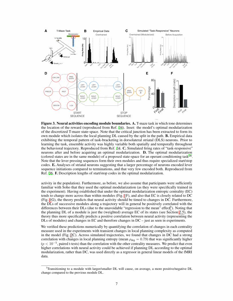
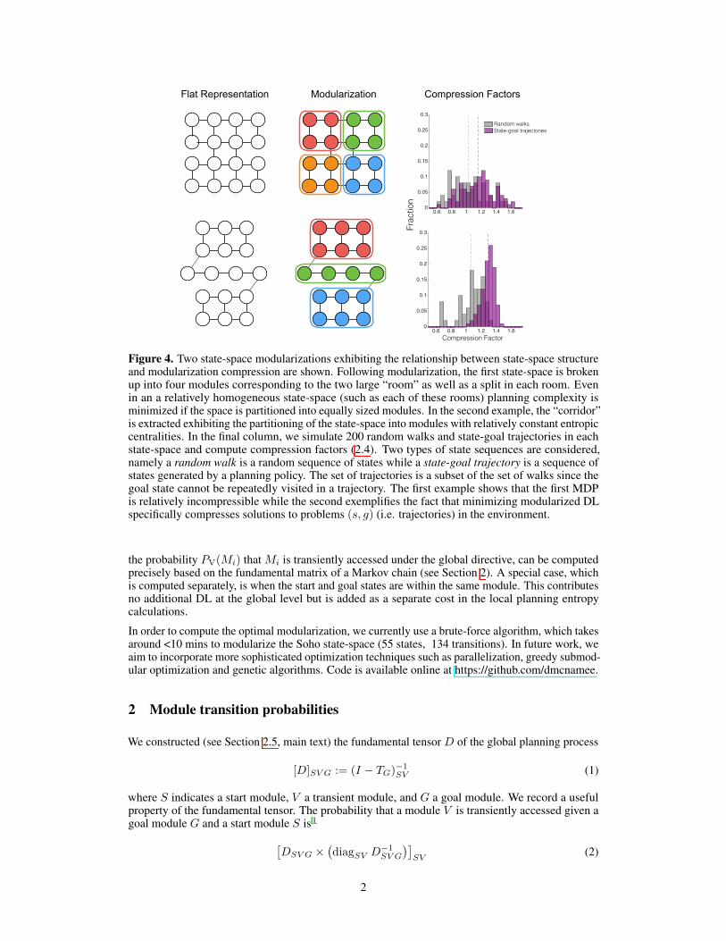