Embed Size (px)
Citation preview
Efficient Storage Design and Query Scheduling for ImprovingBig Data Retrieval and Analytics
by
Zhuo Liu
A dissertation submitted to the Graduate Faculty ofAuburn University
in partial fulfillment of therequirements for the Degree of
Doctor of Philosophy
Auburn, AlabamaMay 9, 2015
Keywords: Big Data, Cloud Computing, Hadoop, Hive Query Scheduling, Phase ChangeMemory, Parallel I/O
Copyright 2015 by Zhuo Liu
Approved by
Weikuan Yu, Chair, Associate Professor of Computer Science and Software EngineeringSaad Biaz, Professor of Computer Science and Software Engineering
Xiao Qin, Associate Professor of Computer Science and Software Engineering
Abstract
With the perpetually increasing requirement and generation of digital data, the human being
has been stepping into the Big Data era. To efficiently manage, retrieve and exploit such gigantic
amount of data continuously generated by all individuals and organizations of the society, a rich set
of efforts has been invested to develop high-performance, scalable and fault-tolerant data storage
systems and analytics frameworks. Recently, flash-based solid state disks and byte-addressable
non-volatile memories have been developed and introduced into computer system storage hier-
archy for substituting traditional hard drives and DRAM due to the faster data accesses, higher
density and energy-efficiency. Along with the trend, how to systematically integrate such cutting
edge memory technologies for fast system data retrieval becomes a highly concerned issue. In
addition, from the users’ point of view, some mission-critical scientific applications are suffering
from inefficient I/O schemes, thus not able to fully utilize the underlying parallel storage systems.
This fact makes the development of more efficient I/O methods appealing. Moreover, MapReduce
has emerged as a powerful big data processing engine that supports large-scale complex analytics
applications. Most of them are written in declarative query languages such as Hive and Pig Latin.
Therefore, it requires efficient coordination of Hive compiler and Hadoop runtime for fast and fair
big data analytics.
This dissertation investigates the research challenges mentioned above and contributes effi-
cient storage design, I/O methods and query scheduling for improving big data retrieval and ana-
lytics. I firstly aim at addressing the I/O bottleneck issue in large-scale computers and data centers.
Accordingly, in my first study, by leveraging the advanced features of cutting-edge non-volatile
memories, I have presented and devised a Phase Change Memory (PCM)-based hybrid storage
architecture, which provides efficient buffer management and novel wear leveling techniques, thus
achieving highly improved data retrieval performance and at the same time solving the PCM’s
ii
endurance issue. In the second study, we adopt a mission-critical scientific application, GEOS-5,
as a case to profile and analyze the communication and I/O issues that are preventing applications
from fully utilizing the underlying parallel storage systems. Through detailed architectural and
experimental characterization, we observe that current legacy I/O schemes incur significant net-
work communication overheads and are unable to fully parallelize the data access, thus degrading
applications’ I/O performance and scalability. To address these inefficiencies, we redesign its I/O
framework along with a set of parallel I/O techniques to achieve high scalability and performance.
In the third study, I have identified and profiled important performance and fairness issues existing
in current MapReduce-based data warehousing system. In particular, I have proposed a prediction
based query scheduling framework, which bridges the semantic gap between MapReduce runtime
and query compiler and enables efficient query scheduling for fast and fair big data analytics.
iii

Acknowledgments
First and foremost, I would like to sincerely thank my advisor, Dr. Weikuan Yu, for his
thorough academic guidance, patient cultivation, encouragement and continuous support during
my doctoral study. I have been really fortunate to become his student and conduct interesting and
cutting-edge research work in the outstanding academic environment he created in the PASL lab.
As my advisor, he has been helping me identify novel research topics and solve critical challenges,
and giving me all kinds of precious opportunities to hone my skills, broaden my horizons and
shape my professional career. He has also been a most helpful friend of me, helping me in my life
and encouraging me during the tough moments. I greatly appreciate his priceless time and efforts
for nurturing me during my Ph.D experience.
I wish to thank my collaborators. It has been my true pleasure to work closely with Dr. Jay
Lofstead in the Sandia National Laboratories during my summer intern, with Dr. Xiaoning Ding
from New Jersey Institute of Technology on the prediction-based query scheduling project, with
Dr. Jeffrey Vetter and Dr. Dong Li from Oak Ridge National Laboratory on the non-volatile
memory project.
I would also like to thank my committee members: Dr. Saad Biaz and Dr. Xiao Qin and
my university reader Dr. Fadel Megahed. Their precious suggestions and patient guidance help to
improve my dissertation.
I feel really grateful to my PASL group-mates: Dr. Yandong Wang, Dr. Yuan Tian, Dr. Xinyu
Que, Cong Xu, Bin Wang, Teng Wang, Patrick Carpenter, Fang Zhou, Huansong Fu, Xinning
Wang, Kevin Vasko, Michael Pritchard, Hai Pham and Bhavitha Ramaiahgari. Their cooperation
in work and help in life make Auburn PASL a big and warm family and an excellent place where
we learn, create, improve and enjoy.
iv

Finally, I own the deepest gratitude to my mother Cui’e Ding, my grandma Yulian Zhang, my
father Jiannong Liu, my grandpa Dirong Liu, my brother Jia Liu, my aunt Zhenfei Liu, my uncle
Minxiang Zhou, my parents-in-law Tianqiao Chen and Zhixiang Cao, and my niece Ziyi Liu for
their unconditional support, care and love. Eventually, I would like to say thank you to my wife
Lin Cao for her everlasting love during my life. Without her being with me, I could not imagine
how I could have gone through such a long journey.
v
Table of Contents
Abstract . . . . . . . . . . . . . . . . . . . . . . . . . . . . . . . . . . . . . . . . . . . . . ii
Acknowledgments . . . . . . . . . . . . . . . . . . . . . . . . . . . . . . . . . . . . . . . . iv
List of Figures . . . . . . . . . . . . . . . . . . . . . . . . . . . . . . . . . . . . . . . . . . ix
List of Tables . . . . . . . . . . . . . . . . . . . . . . . . . . . . . . . . . . . . . . . . . . xii
1 Introduction . . . . . . . . . . . . . . . . . . . . . . . . . . . . . . . . . . . . . . . . 1
1.1 Research Background . . . . . . . . . . . . . . . . . . . . . . . . . . . . . . . . . 2
1.1.1 Background of Non-Volatile Memories . . . . . . . . . . . . . . . . . . . 2
1.1.2 Background of Scientific I/O . . . . . . . . . . . . . . . . . . . . . . . . . 3
1.1.3 Background of MapReduce-based Data Warehouse Systems . . . . . . . . 4
1.2 Research Contributions . . . . . . . . . . . . . . . . . . . . . . . . . . . . . . . . 5
1.2.1 PCM-Based Hybrid Storage . . . . . . . . . . . . . . . . . . . . . . . . . 5
1.2.2 I/O Framework Optimization for GEOS-5 . . . . . . . . . . . . . . . . . . 6
1.2.3 Prediction Based Two-Level Query Scheduling . . . . . . . . . . . . . . . 8
1.3 Publications . . . . . . . . . . . . . . . . . . . . . . . . . . . . . . . . . . . . . . 8
1.4 Dissertation Overview . . . . . . . . . . . . . . . . . . . . . . . . . . . . . . . . 10
2 Problem Statement . . . . . . . . . . . . . . . . . . . . . . . . . . . . . . . . . . . . 12
2.1 Challenges in I/O Systems for Exascale Computers . . . . . . . . . . . . . . . . . 12
2.2 Challenges in big data retrieval for scientific applications . . . . . . . . . . . . . . 13
2.2.1 Current Data Aggregation and I/O in GEOS-5 . . . . . . . . . . . . . . . . 13
2.2.2 Issues with the Existing Approach . . . . . . . . . . . . . . . . . . . . . . 14
2.2.3 Performance Dissection of Communication and I/O . . . . . . . . . . . . . 16
2.3 Performance and Fairness Issues Caused by Semantic Unawareness . . . . . . . . 17
2.3.1 Execution Stalls of Concurrent Queries . . . . . . . . . . . . . . . . . . . 17
vi
2.3.2 Query Unfairness . . . . . . . . . . . . . . . . . . . . . . . . . . . . . . . 18
3 PCM Based Hybrid Storage . . . . . . . . . . . . . . . . . . . . . . . . . . . . . . . . 21
3.1 Design for PCM Based Hybrid Storage . . . . . . . . . . . . . . . . . . . . . . . . 21
3.1.1 HALO Framework and Data Structures . . . . . . . . . . . . . . . . . . . 22
3.1.2 HALO Caching Scheme . . . . . . . . . . . . . . . . . . . . . . . . . . . 26
3.1.3 Two-Way Destaging . . . . . . . . . . . . . . . . . . . . . . . . . . . . . 27
3.2 Wear Leveling for PCM . . . . . . . . . . . . . . . . . . . . . . . . . . . . . . . . 29
3.2.1 Rank-Bank Round-Robin Wear Leveling . . . . . . . . . . . . . . . . . . 30
3.2.2 Space Fill Curve Based Wear leveling . . . . . . . . . . . . . . . . . . . . 30
3.3 Evaluation for PCM-Based Hybrid Storage . . . . . . . . . . . . . . . . . . . . . 33
3.3.1 I/O Performance . . . . . . . . . . . . . . . . . . . . . . . . . . . . . . . 36
3.3.2 Wear Leveling Results . . . . . . . . . . . . . . . . . . . . . . . . . . . . 39
3.4 Related Studies on Hybrid Storage and NVM . . . . . . . . . . . . . . . . . . . . 41
3.5 Summary . . . . . . . . . . . . . . . . . . . . . . . . . . . . . . . . . . . . . . . 45
4 I/O Optimization for a Large-Scale Climate Scientific Application . . . . . . . . . . . 46
4.1 An Extensible Parallel I/O Framework . . . . . . . . . . . . . . . . . . . . . . . . 46
4.1.1 A Generalized and Portable Architecture . . . . . . . . . . . . . . . . . . 46
4.1.2 Leveraging Parallel NetCDF . . . . . . . . . . . . . . . . . . . . . . . . . 47
4.1.3 Integration of ADIOS . . . . . . . . . . . . . . . . . . . . . . . . . . . . 48
4.2 Experimental Evaluation . . . . . . . . . . . . . . . . . . . . . . . . . . . . . . . 49
4.2.1 Performance with PnetCDF . . . . . . . . . . . . . . . . . . . . . . . . . 49
4.2.2 Performance with ADIOS . . . . . . . . . . . . . . . . . . . . . . . . . . 51
4.3 Related Studies on I/O optimizations for scientific applications . . . . . . . . . . . 53
4.4 Summary . . . . . . . . . . . . . . . . . . . . . . . . . . . . . . . . . . . . . . . 54
5 Prediction Based Two-Level Query Scheduling . . . . . . . . . . . . . . . . . . . . . 55
5.1 Cross-layer Scheduling Framework . . . . . . . . . . . . . . . . . . . . . . . . . . 55
5.2 Query prediction model . . . . . . . . . . . . . . . . . . . . . . . . . . . . . . . . 57
vii
5.2.1 Selectivity Estimation . . . . . . . . . . . . . . . . . . . . . . . . . . . . 57
5.2.2 A Multivariate Regression Model . . . . . . . . . . . . . . . . . . . . . . 62
5.3 Two-level Query Scheduling . . . . . . . . . . . . . . . . . . . . . . . . . . . . . 66
5.3.1 Inter-Query Scheduling . . . . . . . . . . . . . . . . . . . . . . . . . . . . 66
5.3.2 Intra-Query Scheduling . . . . . . . . . . . . . . . . . . . . . . . . . . . . 69
5.4 Evaluation for MapReduce Query Scheduling . . . . . . . . . . . . . . . . . . . . 72
5.4.1 Experimental Settings . . . . . . . . . . . . . . . . . . . . . . . . . . . . 73
5.4.2 Intra-Query Scheduling Evaluation . . . . . . . . . . . . . . . . . . . . . 74
5.4.3 Overall Performance . . . . . . . . . . . . . . . . . . . . . . . . . . . . . 77
5.5 Related Studies on MapReduce and Scheduling . . . . . . . . . . . . . . . . . . . 83
5.5.1 Query Modeling . . . . . . . . . . . . . . . . . . . . . . . . . . . . . . . 83
5.5.2 MapReduce Scheduling and Other Related Work . . . . . . . . . . . . . . 84
5.6 Summary . . . . . . . . . . . . . . . . . . . . . . . . . . . . . . . . . . . . . . . 86
6 Conclusion . . . . . . . . . . . . . . . . . . . . . . . . . . . . . . . . . . . . . . . . 87
7 Future Plan . . . . . . . . . . . . . . . . . . . . . . . . . . . . . . . . . . . . . . . . 89
Bibliography . . . . . . . . . . . . . . . . . . . . . . . . . . . . . . . . . . . . . . . . . . 91
viii
List of Figures
2.1 Overview of GEOS-5 Communication and I/O . . . . . . . . . . . . . . . . . . . . . 13
2.2 I/O Scalability of Original GEOS-5 . . . . . . . . . . . . . . . . . . . . . . . . . . . 15
2.3 Time Dissection of Non-blocking MPI Communication . . . . . . . . . . . . . . . . . 16
2.4 Time Dissection for Collecting and Storing Bundles . . . . . . . . . . . . . . . . . . . 16
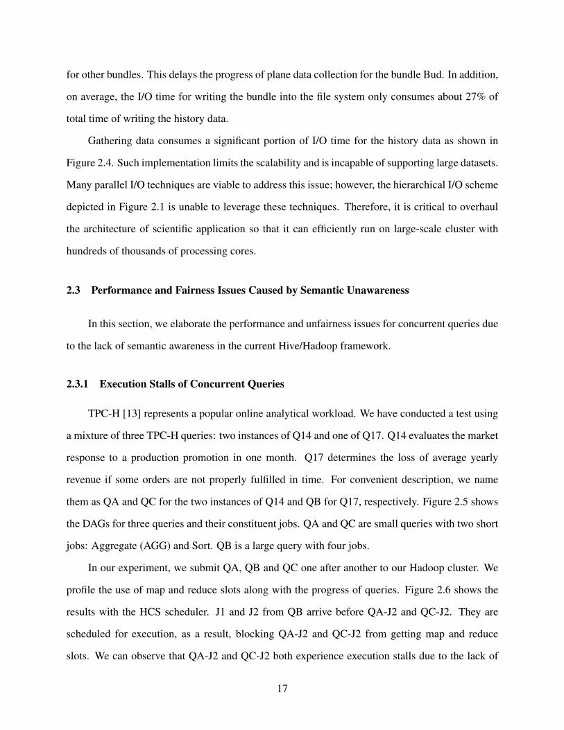
2.5 A Diagram of Jobs in the DAGs of Three Queries . . . . . . . . . . . . . . . . . . . . 18
2.6 Execution Stalls of Queries with HCS . . . . . . . . . . . . . . . . . . . . . . . . . . 19
2.7 Chain Query Group and Tree Query Group . . . . . . . . . . . . . . . . . . . . . . . 19
2.8 Fairness to Queries of Different Compositions . . . . . . . . . . . . . . . . . . . . . . 20
3.1 Different architectures of hybrid storage devices . . . . . . . . . . . . . . . . . . . . . 21
3.2 Design of the HALO framework . . . . . . . . . . . . . . . . . . . . . . . . . . . . . 23
3.3 Data structures of HALO caching . . . . . . . . . . . . . . . . . . . . . . . . . . . . 24
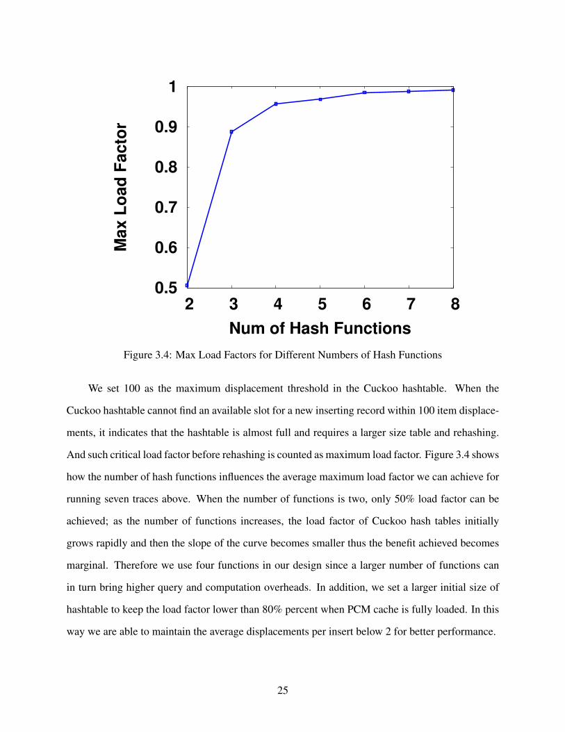
3.4 Max Load Factors for Different Numbers of Hash Functions . . . . . . . . . . . . . . 25
3.5 Rank-bank round-robin wear leveling . . . . . . . . . . . . . . . . . . . . . . . . . . 31
3.6 Space filling curve based wear leveling . . . . . . . . . . . . . . . . . . . . . . . . . 32
3.7 PCM Simulation and Trace Replay . . . . . . . . . . . . . . . . . . . . . . . . . . . . 34
ix
3.8 Execution time . . . . . . . . . . . . . . . . . . . . . . . . . . . . . . . . . . . . . . 35
3.9 Traffic rate for Fin1, Fin2 and Dap . . . . . . . . . . . . . . . . . . . . . . . . . . . . 36
3.10 Traffic rate for Exchange, TPC-E, Mail and Randw . . . . . . . . . . . . . . . . . . . 37
3.11 Average inter-request LBN distance . . . . . . . . . . . . . . . . . . . . . . . . . . . 38
3.12 HDD throughput rate and HALO’s improvement over LRU . . . . . . . . . . . . . . . 39
3.13 Original LBN distribution of Fin1 . . . . . . . . . . . . . . . . . . . . . . . . . . . . 40
3.14 LBN distribution of Fin1 after applying the HALO caching . . . . . . . . . . . . . . . 41
3.15 Response time . . . . . . . . . . . . . . . . . . . . . . . . . . . . . . . . . . . . . . 42
3.16 Life ratio comparison between different wear leveling techniques . . . . . . . . . . . . 43
3.17 Write deviations among banks for Fin2 . . . . . . . . . . . . . . . . . . . . . . . . . 44
4.1 Parallel I/O Based System Architecture . . . . . . . . . . . . . . . . . . . . . . . . . 47
4.2 Comparison between Serial NetCDF and PnetCDF . . . . . . . . . . . . . . . . . . . 50
4.3 Time dissection of CFIO and PnetCDF . . . . . . . . . . . . . . . . . . . . . . . . . 51
4.4 Comparison between CFIO and ADIOS . . . . . . . . . . . . . . . . . . . . . . . . . 52
4.5 Time Dissection of ADIOS-MPI . . . . . . . . . . . . . . . . . . . . . . . . . . . . . 52
5.1 Prediction-Based Two-Level Scheduling Framework . . . . . . . . . . . . . . . . . . 55
5.2 Intermediate and Final Selectivity Estimation . . . . . . . . . . . . . . . . . . . . . . 58
5.3 An Example of Selectivity Estimation . . . . . . . . . . . . . . . . . . . . . . . . . . 62
x
5.4 Accuracy of Job Execution Prediction . . . . . . . . . . . . . . . . . . . . . . . . . . 64
5.5 Accuracy of Query Response Time Prediction . . . . . . . . . . . . . . . . . . . . . . 65
5.6 Comparison between HLFET and DFA Algorithms . . . . . . . . . . . . . . . . . . . 70
5.7 An Example of Table Sharing for a TPC-H Query . . . . . . . . . . . . . . . . . . . . 72
5.8 Query Response Times of Q9, Q18, Q17, and Q21 when They Use System Resources
Alone. . . . . . . . . . . . . . . . . . . . . . . . . . . . . . . . . . . . . . . . . . . . 75
5.9 Query Response Times of 5 Instances of Q21 with Different Input Sizes. . . . . . . . . 76
5.10 CDF of Query Response Time in Bing Workload . . . . . . . . . . . . . . . . . . . . 79
5.11 CDF of Query Response Time in Facebook Workload . . . . . . . . . . . . . . . . . . 79
5.12 Aggregated stall times of the query bins in Bing and Facebook workloads (the times
are in the logarithmic scale). . . . . . . . . . . . . . . . . . . . . . . . . . . . . . . . 80
5.13 Maximum Slowdown . . . . . . . . . . . . . . . . . . . . . . . . . . . . . . . . . . . 81
5.14 Average Slowdown . . . . . . . . . . . . . . . . . . . . . . . . . . . . . . . . . . . . 82
xi
List of Tables
3.1 Parameters Used for Wear Leveling. . . . . . . . . . . . . . . . . . . . . . . . . . . . 29
3.2 Workload Statistics . . . . . . . . . . . . . . . . . . . . . . . . . . . . . . . . . . . . 35
3.3 The Effects of Cuckoo Hash Function Numbers on Load Factors . . . . . . . . . . . . 36
3.4 Wear leveling Results . . . . . . . . . . . . . . . . . . . . . . . . . . . . . . . . . . . 40
5.1 Input Features for the Model . . . . . . . . . . . . . . . . . . . . . . . . . . . . . . . 63
5.2 Accuracy Statistics for Job Execution Prediction . . . . . . . . . . . . . . . . . . . . 65
5.3 Accuracy for Task Execution Prediction . . . . . . . . . . . . . . . . . . . . . . . . . 67
5.4 Workload Characteristics . . . . . . . . . . . . . . . . . . . . . . . . . . . . . . . . . 73
5.5 Average Query Response Times . . . . . . . . . . . . . . . . . . . . . . . . . . . . . 78
xii
Chapter 1
Introduction
As reported by IDC [39], the digital universe (a measure of all digital data generated, created
and consumed in a single year) will rise from about 3,000 exabytes in 2012 to 40,000 exabytes
in 2020. To cope with the booming storage and retrieval requirement of such gigantic data, nu-
merous endeavors have been invested. Flash based solid-state devices (FSSDs) have been adopted
within the memory hierarchy to improve the performance of hard disk drive (HDD) based storage
system. However, with the fast development of storage-class memories, new storage technologies
with better performance and higher write endurance than FSSDs are emerging, e.g., phase-change
memory (PCM) [6]. Understanding how to leverage these state-of-the-art storage technologies for
modern computing systems is important to solve challenging data intensive computing problems.
Even equipped with highly parallel underlying storage systems, some legacy important sci-
entific applications are still being impeded by inefficient I/O aggregation and output schemes. In
order to represent the scientific information ranging from physics, chemistry to biology on dif-
ferent longitudes, latitudes and altitudes all over the earth, huge amounts of multi-dimension data
sets need to be produced, stored and accessed in an efficient way. However, quite a few impor-
tant applications still lack efficient I/O methods to deal with such data retrieval issues efficiently.
GEOS-5 [8] is one of such applications.
Moreover, 33% of data in the digital universe can be valuable if analyzed [39]. However,
currently only 0.5% of total data have been analyzed due to limited analytic capabilities. Thus
it requires highly efficient, scalable and flexible approaches to conduct analytics on such gigan-
tic data, where cloud computing plays an increasingly important role. MapReduce [29] is a very
popular programming model widely used for efficient, scalable and fault-tolerant data analytics.
1

In addition, to ease the coding difficulties for each individual MapReduce job, a set of data ware-
house systems and query languages are exploited on top of the MapReduce framework, such as
Hive [94], Pig [40] and DryadLINQ [117]. In MapReduce based data warehousing system, an-
alytic queries are typically compiled into execution plans in the form of directed acyclic graphs
(DAGs) of MapReduce jobs. Jobs in the DAGs are dispatched to the MapReduce processing en-
gine as soon as their dependencies are satisfied. MapReduce adopts a task-level scheduling policy
to strive for balanced distribution of tasks and effective utilization of resources. However, there is
a lack of query-level semantics in the purely task-based scheduling algorithms, resulting in unfair
treatment of different queries, low utilization of system resources, prolonged execution time, and
low query throughput.
In this dissertation, I present our studies of PCM-based hybrid storage, I/O optimization for
scientific applications, and MapReduce query scheduling framework for improving big data re-
trieval and analytics. In the rest of this chapter, I first provide a background introduction for my
studies. I then give an introduction for my major research contributions. At the end, I provide a
brief overview of this dissertation.
1.1 Research Background
1.1.1 Background of Non-Volatile Memories
The explosive growth of data brings both performance and power consumption challenges. To
solve these challenges, flash-based Hybrid Storage Drives (HSDs) have been proposed to combine
standard hard disk drives (HDDs) and Flash-based Solid-State Drives (FSSDs) into a single storage
enclosure [4]. Although flash-based HSDs are gaining popularity, they suffer from several striking
shortcomings of FSSDs, namely high write latency and low endurance, which seriously hinder the
successful integration of FSSDs into HSDs. Lots of techniques have been proposed to address the
issues [90, 88]. However, most of them only target specific usage scenarios and cannot act as a
general solution to eliminate FSSDs’ drawbacks, which continue to threaten the future success of
FSSD-based HSDs. There remains a need of better technologies in the storage market.
2
Latest storage technologies are bringing in new non-volatile random-access memory (NVRAM)
devices such as phase-change memory, spin-torque transfer memory (STTRAM) [57], and resis-
tive RAM (RRAM) [57]. These memory devices support the non-volatility of conventional HDDs
while providing speeds approaching those of DRAMs. Among these technologies, PCM is par-
ticularly promising with several companies and universities already providing prototype chips and
devices [18, 6]. Compared to FSSD, PCM is equipped with a number of performance and en-
ergy advantages [26]. First, PCM has much faster read response time than FSSD. It offers a read
response time of around 50ns, nearly 500 times faster than that of FSSD. Second, PCM can over-
write data directly on the memory cell, unlike FSSD’s write-after-erase. The write response time
of PCM is less than 1 us, nearly three orders of magnitude faster than that of FSSD. Third, the
program energy for PCM is 6 Joule/GB, 3 times smaller than that of FSSD [26]. Thus, PCM is a
viable alternative to FSSDs for building hybrid storage systems.
A number of techniques have used NVRAM as data cache to improve disk I/O [20, 33, 55,
101, 41]. Most of them use LRU-like methods (e.g., Least Recently Written, LRW [33, 41])
to manage small size non-volatile cache to improve performance and reliability of HDD-based
storage and file system. However, for GBs of high density PCM cache, using LRU to manage
them will cause big DRAM overheads in managing the LRU stack and mapping. In addition,
LRU/LRW cannot ensure that destaging I/O traffic be presented as sequential writes to hard disks.
CSCAN method used in [41] as a supplement for LRW can ease this issue to some extent but
it requires O(log(n)) time for insertion, making it not suitable for large size cache management.
Therefore, it is crucial to rethink the current cache management strategies for PCM.
1.1.2 Background of Scientific I/O
Scientific applications are playing a critical role in improving our daily life. They are de-
signed to solve pressing scientific challenges, including designing new energy-efficient sources [5]
3
and modeling the earth system [8]. To boost the productivity of scientific applications, High-
Performance Computing (HPC) community has built many supercomputers [12] with unprece-
dented computation power over the past decade. Meanwhile, computer scientists are also arduously
improving parallel file systems [28, 83] and I/O techniques [66, 67] to bridge the gap between fast
processors and slow storage systems. Despite the rapid evolution of HPC infrastructures, the de-
velopment of scientific applications dramatically lags behind in leveraging the capabilities of the
underlying systems, especially the superior I/O performance.
1.1.3 Background of MapReduce-based Data Warehouse Systems
Analytics applications often impose diverse yet conflicting requirements on the performance
of underlying MapReduce systems, such as high throughput, low latency, and fairness among jobs.
For example, to support latency-sensitive applications from advertisements and real-time event log
analysis, MapReduce must provide fast turnaround time.
Because of their declarative nature and ease of programming, analytics applications are often
created using high-level query languages. These analytic queries are transformed by compilers into
an execution plan of multiple MapReduce jobs, which are often depicted as direct acyclic graphs
(DAGs). A job in a DAG can only be submitted to MapReduce when its dependencies are satisfied.
A DAG query completes when its last job is finished. Thus the execution of analytic queries is
centered around dependencies among DAG jobs and the completion of jobs along the critical path
of a DAG. On the other hand, to support MapReduce jobs from various sources, the lower level
MapReduce systems usually adopt a two-phase scheme that allocates computation, communication
and I/O resources to two types of constituent tasks (Map and Reduce) from concurrently active
jobs. For example, the Hadoop Fair Scheduler (HFS) and Capacity Scheduler (HCS) strive to
allocate resources among map and reduce tasks to aim for good fairness among different jobs
and high throughput of outstanding jobs. When a job finishes, the schedulers immediately select
tasks from another job for resource allocation and execution. However, these two jobs may belong
4
to DAGs of two different queries. Such interleaved execution of jobs from different queries can
significantly delay the completion of all involved queries, as we will show in Chapter 2.3.
This scenario is a manifestation of the mismatch between system and application objectives.
While the schedulers in the MapReduce processing engine focus on the job-level fairness and
throughput, analytic applications are mainly concerned with the query-level performance objec-
tives. This mismatch of objectives often leads to prolonged execution of user queries, resulting in
poor user satisfaction. Besides the delayed query completion, the existing schedulers in MapRe-
duce also have difficulties in recognizing the locality of data across jobs. For example, jobs in
the same DAG may share their input data [118]. But Hadoop schedulers are unable to detect the
existence of common data among these jobs and may schedule them with a long lapse of time. In
this case, the same data would be read multiple times, degrading the throughput of MapReduce
systems. As Hive and Pig Latin have been used pervasively in data warehouses, the above problem
becomes a serious issue and must be timely addressed. More than 40% of Hadoop production
jobs at Yahoo! have been Pig programs [40]. In Facebook, 95% Hadoop jobs are generated by
Hive [56].
1.2 Research Contributions
1.2.1 PCM-Based Hybrid Storage
In this dissertation, I design a novel hybrid storage system that leverages PCM as a write
cache to merge random write requests and improve access locality for HDDs. To support this
hybrid architecture, I propose a novel cache management algorithm, named HALO. It implements
a new eviction policy and manages address mapping through cuckoo hash tables. These techniques
together save DRAM overheads significantly while maintaining constant O(1) speeds for both
insertion and query. Furthermore, HALO is very beneficial in terms of managing caching items,
merging random write requests, and improving data access locality. In addition, by removing the
dirty-page write-back limitations that commonly exist in DRAM-based caching systems, HALO
enables better write caching and destaging, and thus achieves better I/O performance. And by
5
storing cache mapping information on non-volatile PCM, the storage system is able to recover
quickly and maintain integrity in case of system crashes.
To use PCM as a write cache, I also address PCM’s limited durability. Several existing
wear-leveling techniques have shown good endurance improvement for PCM-based memory sys-
tems [78, 77, 122]. However, these techniques are not specifically designed for PCM used in
storage and file systems, and thus can negatively impact spatial locality of file system accesses,
which in turn will degrade read-ahead and sequential access performance of file systems. I pro-
pose a wear leveling technique called space filling curve wear-leveling, which not only provides a
good write balance between different regions of the device, but also keeps data locality and enables
good adaptation to the file system’s I/O access characteristics.
Using two in-house simulators, I have evaluated the functionality of the proposed PCM-based
hybrid storage devices. Our experimental results demonstrate that the HALO caching scheme leads
to an average reduction of 36.8% in execution time compared to the LRU caching scheme, and that
the SFC wear leveling extends the lifetime of PCM by a factor of 21.6. Our results demonstrate
that PCM can serve as a write cache for fast and durable hybrid storage devices.
1.2.2 I/O Framework Optimization for GEOS-5
This paper seeks to examine and characterize the communication and I/O issues that prevent
current scientific applications from fully exploiting the I/O bandwidth provided by underneath
parallel file systems. Based on our detailed analysis, we propose a new framework for scientific
applications to support a rich set of parallel I/O techniques. Among different applications, we
select the Goddard Earth Observing System model, Version 5, (GEOS-5) from NASA [8] as a
representative case. GEOS-5 is a large-scale scientific application designed for grand missions
such as climate modeling, weather broadcasting and air-temperature simulation. Built on top of
Earth System Modeling Framework (ESMF) [42] and MAPL library [89], GEOS-5 incorporates a
system of models to conduct NASA’s earth science research, such as observing Earth systems, and
climate and weather prediction.
6
GEOS-5 contains various communication and I/O patterns observed in many applications for
check-pointing and writing output. Data are organized in the form of either 2 or 3 dimensional
variables. In many cases, multiple variables are arranged in the same group, called a bundle. A
single variable is a composition of a number of 2-D planes, each of which is evenly partitioned
among all the processes in the same application. Although the computation can be fully par-
allelized, our characterization identifies three inefficient communication and I/O patterns in the
current design. First, for each plane of data, a process has to be elected as the plane root to gather
all the data from all processes in the plane, thus causing a single point of contention. Second, only
one process, called the bundle root, is responsible for collecting data from all the plane roots and
writing the entire bundle to the storage system. This behavior essentially forces all the processes
to wait until the bundle root finishes I/O, resulting in not only an I/O bottleneck but also a severe
global synchronization barrier. Third, GEOS-5, like many legacy scientific applications, is unable
to leverage state-of-the-art parallel I/O techniques due to rigid framework constraints, and continue
using serial I/O interfaces, such as serial NetCDF (Network Common Data Form) [9].
To address the above inefficiencies, we redesign the communication and I/O framework in this
GEOS-5 application, so that the new framework can allow application to exploit the performance
advantages provided by a rich set of parallel I/O techniques. However, our experimental evaluation
shows that simply using parallel I/O tools such as PnetCDF [58], cannot effectively enable appli-
cation to scale to a large number of processes due to metadata synchronization overhead. On the
other hand, using another parallel I/O library, called ADIOS (The Adaptable IO System) [66], can
improve the I/O performance with the trade-off that it may sacrifice the consistency induced by
delayed inter-process written synchronization and complicate the post processing of output files.
To summarize, we have made following three research contributions in this work:
• We conduct a comprehensive analysis of a climate scientific application, GEOS-5, and iden-
tify several performance issues with GEOS-5 communication and I/O patterns.
• We design a new parallel framework in GEOS-5 for it to leverage a variety of parallel I/O
techniques.
7
• We have employed PnetCDF and ADIOS for alternative I/O solutions for GEOS-5 and eval-
uated their performance. Our evaluation demonstrates that our optimization with ADIOS
can significantly improve the I/O performance of GEOS-5.
1.2.3 Prediction Based Two-Level Query Scheduling
In this dissertation, I propose a prediction-based two-level scheduling framework that can
address these problems systematically. Three techniques are introduced including cross-layer se-
mantics percolation, selectivity estimation and multivariate time prediction, and two-level query
scheduling (TLS for brevity). First, cross-layer semantics percolation allows the flow of query
semantics and job dependencies in the DAG to the MapReduce scheduler. Second, with rich se-
mantics information, I model the changing size of analytics data through selectivity estimation,
and then build a multivariate model that can accurately predict the execution time of individual
jobs and queries. Furthermore, based on the multivariate time predication, I introduce two-level
query scheduling that can maximize the intra-query job-level concurrency, speed up the query
completion, and ensure query fairness.
Our experimental results on a set of complex workloads demonstrate that TLS can signifi-
cantly improve both fairness and throughput of Hive queries. Compared to HCS and HFS, TLS
improves average query response time by 43.9% and 27.4% for the Bing benchmark and 40.2%
and 72.8% for the Facebook benchmark. Additionally, TLS achieves 59.8% better fairness than
HFS on average.
1.3 Publications
During my doctoral study, my research work has contributed to the following publications.
1. Z. Liu, W. Yu, F. Zhou, X. Ding and W. Tsai. Prediction-Based Two-Level Scheduling for
Analytic Queries. Under review.
8
2. Z. Liu, B. Wang and W. Yu. HALO: A Fast and Durable Disk Write Cache using Phase
Change Memory. Journal of Cluster Computing (Springer). Under minor revision.
3. C. Xu, R. Goldsone, Z. Liu, H. Chen, B. Neitzel and W. Yu. Exploiting Analytics Ship-
ping with Virtualized MapReduce on HPC Backend Storage Servers. IEEE Transactions on
Parallel and Distributed Computing, 2015 [25].
4. T. Wang, K. Vasko, Z. Liu, H. Chen, and W. Yu. Enhance Scientific Application I/O with
Cross-Bundle Aggregation. International Journal of High Performance Computing Applica-
tions, 2015 [105].
5. X. Wang, B. Wang, Z. Liu and W. Yu. ”Preserving Row Buffer Locality for PCM Wear-
Leveling Under Massive Parallelism. Under review.
6. B. Wang, Z. Liu, X. Wang and W. Yu. Eliminating Intra-Warp Conflict Misses in GPU. In
IEEE Design, Automation and Test in Europe (DATE), 2015 [102].
7. T. Wang, K. Vasko, Z. Liu, H. Chen, and W. Yu. BPAR: A Bundle-Based Parallel Aggre-
gation Framework for Decoupled I/O Execution. International Workshop on Data-Intensive
Scalable Computing Systems (DISCS), 2014 [104].
8. Z. Liu, J. Lofstead, T. Wang, and W. Yu. A Case of System-Wide Power Management for
Scientific Applications. In IEEE International Conference on Cluster Computing, 2013 [62].
9. Z. Liu, B. Wang, T. Wang, Y. Tian, C. Xu, Y. Wang, W. Yu, C. Cruz, S. Zhou, T. Clune
and S. Klasky. Profiling and Improving I/O Performance of a Large-Scale Climate Scien-
tific Application. In International Conference on Computer Communications and Networks
(ICCCN), 2013 [63].
9
10. Y. Tian, Z. Liu, S. Klasky, B. Wang, H. Abbasi, S. Zhou, N. Podhorszki, T. Clune, J. Logan,
and W. Yu. A Lightweight I/O Scheme to Facilitate Spatial and Temporal Queries of Sci-
entific Data Analytics. In IEEE Symposium on Massive Storage Systems and Technologies
(MSST), 2013 [97].
11. C. Xu, M. G. Venkata, R. L. Graham, Y. Wang, Z. Liu and W. Yu. SLOAVx: Scalable
LOgarithmic AlltoallV Algorithm for Hierarchical Multicore Systems. In IEEE/ACM Inter-
national Symposium on Cluster, Cloud and Grid Computing (CCGrid), 2013 [112].
12. Y. Wang, Y. Jiao, C. Xu, X. Li, T. Wang, X. Que, C. Cira, B. Wang, Z. Liu, B. Bailey and
W. Yu. Assessing the Performance Impact of High-Speed Interconnects on MapReduce. In
Third Workshop on Big Data Benchmarking (Invited Book Chapter), 2013 [106].
13. Z. Liu, B. Wang, P. Carpenter, D. Li, J. Vetter and W. Yu. PCM-Based Durable Write Cache
for Fast Disk I/O. In IEEE International Symposium on Modeling, Analysis and Simulation
of Computer and Telecommunication Systems (MASCOTS), 2012 [61].
14. D. Li, J.S. Vetter, G. Marin, C. McCurdy, C. Cira, Z. Liu, W. Yu. Identifying opportuni-
ties for byte-addressable non-volatile memory in extreme-scale scientific applications. In
International Parallel and Distributed Processing Symposium (IPDPS), 2012 [57].
15. Z. Liu, J. Zhou, W. Yu, F. Wu, X. Qin and C. Xie. MIND: A Black-Box Energy Consump-
tion Model for Disk Arrays. In 1st International Workshop on Energy Consumption and
Reliability of Storage Systems (ERSS’11), 2011 [64].
1.4 Dissertation Overview
The focus of this dissertation is on efficient storage design and query scheduling for improv-
ing big data retrieval and analytics, which targets at addressing the challenges that origin from
explosive data generation and increasing requirements of fast data accesses and analysis. To be
specific, this dissertation makes the following research contributions:
10
• I design a novel hybrid storage system that leverages PCM as a write cache to merge random
write requests and improve access locality for HDDs. To support this hybrid architecture, I
propose a novel cache management algorithm, named HALO. In addition, I devise two novel
wear leveling technique to prolong PCM’s life time.
• I profile the inefficiency issue in a mission-critical scientific application called GEOS-5 and
address the single point contention and network bottleneck issue by amending its I/O mid-
dleware and enabling the integration of parallel I/O interfaces, through which its I/O perfor-
mance gets significantly improved.
• I design a prediction-based two-level query scheduling framework that can exploit query
semantics for resource and time prediction, thus guiding scheduling decisions at two levels:
the intra-query level for better job parallelism and the inter-query level for fast and fair query
completion.
• Systematic experimental evaluations are conducted to demonstrate our solutions’ advantages
of improving big data retrieval and analytics efficiency over traditional techniques.
The remainder of the dissertation is organized as follows. In Chapter 2, I present the problem
statement, which reveals the challenges in current big data storage and retrieval, and then identifies
performance and fairness issues of MapReduce based data warehouse systems. In Chapter 3, I
detail the design, implementation and evaluation of PCM-based hybrid storage. In Chapter 4, the
design, implementation and evaluation of GEOS-5 I/O optimization are introduced. In Chapter 5,
I describe the design, implementation and evaluation of Prediction Based Two-Level Scheduling.
I summarize the dissertation and point out future research directions in Chapter 6 and Chapter 7.
11
Chapter 2
Problem Statement
In this chapter, I firstly analyze I/O systems’ challenges for exascale computers, then address
and characterize the performance and fairness disadvantages for queries under traditional MapRe-
duce scheduling techniques.
2.1 Challenges in I/O Systems for Exascale Computers
To address existing performance and power consumption issues, a rich set of efforts have
been undertaken to bring faster and more energy efficient computing [10], memory [57] and stor-
age [113] hardware to build large-scale supercomputers.
In terms of memory and storage techniques, the new cutting-edge non-volatile random-access
memory (NVRAM) attracts many people’s focuses. The NVRAM technologies include phase-
change memory (PCM), spin-torque transfer memory (STTRAM) [57], and resistive RAM (RRAM) [57],
which support the non-volatility of conventional HDDs while providing similar speeds and byte
addressability as DRAMs.
Phase-change memory technology has become mature enough to enter the market [18, 6] be-
cause of the new discoveries of fast-crystallizing materials such as Ge2Sb2Te5(GST) and In-doped
Sb2Te(AIST). Phase-change memory (PCM) is based on a type of chalcogenide-based material
made of germanium, antimony or tellurim. The chalcogenide-based material can exist in different
states with dramatically different electrical resistivity. The crystalline and amorphous states are
two typical states. In the crystalline state, the material has a low resistance and is used to represent
a binary 1; while in the amorphous state, the material has a high resistance and is used to represent
a binary 0. However, there’s still a lack of systematic way to integrate such non-volatile memories
12
as PCM into our traditional storage hierarchy for addressing the I/O challenges in future exascale
computers.
2.2 Challenges in big data retrieval for scientific applications
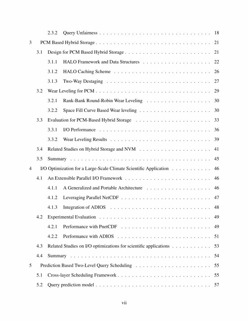
P4
P2
P4
P1 P2
P4
P1 P2
P4 P1
P2
Bundle root
Var 2
Var 3
Var 1
P3
P3
P3
P3 P1
P1
Bundle root receives data layer by layer and writes them to one bundle file. For m bundles, m bundle files will be created at each time step.
Plane root
gather point-to-point
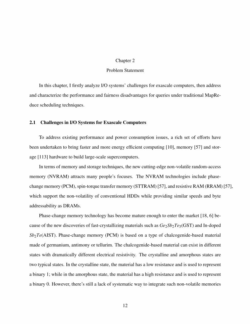
Figure 2.1: Overview of GEOS-5 Communication and I/O
In this section, we first characterize the communication and I/O patterns in GEOS-5, and
then examine their impacts on the application performance. The profiling results suggest that it is
important to explore an alternative design for the data aggregation and storage for GEOS-5.
2.2.1 Current Data Aggregation and I/O in GEOS-5
GEOS-5 is developed by NASA to simulate climate changes over various temporal granular-
ities, ranging from hours to multiple centuries. Like many legacy scientific applications, GEOS-5
adopts the serial version of NetCDF-4 I/O library [9] for managing its simulation data.
Data variables that describe climate systems are organized as bundles, and each bundle rep-
resents a physics model such as moisture and turbulence. It contains a varied mixture of many
13

variables. Each variable has its data organized as a multidimensional dataset, e.g., a 3-D variable
transposing internally into latitude, longitude, and elevation. To describe different aspects of the
model, multiple 2-D or 3-D variables of state physics are defined, such as cloud condensates and
precipitation.
GEOS-5 applies two-dimensional domain decomposition to all variables among parallel pro-
cesses. 2-D variables have only one level of depth, naturally forming a 2D plane. 3-D variables
are organized as multiple 2D planes. The number of 2-D planes is equal to the depth of a 3-D vari-
able. As shown in Figure 2.1, the bundle contains two 2-D variables - var1 and var3 and one 3-D
variable - var2, thus forming a four-layer tube. Each 2-D plane of this bundle is equally divided
among four processes so that all four processes can perform simulation in parallel.
At the end of a timestamp, these state variables are written to the underlying file system as
history data for future analysis (the real production run lasts for tens or hundreds of timestamps).
For maintaining the integrity of the model, all state variables that belong to the same model are
written into the same file, called a bundle file. As mentioned earlier, each bundle file is stored using
the netcdf format [9] popular for climatologists.
GEOS-5 currently adopts a hierarchical scheme for collecting data variables and writing them
into a bundle file. As shown in Figure 2.1, at the first step, each plane designates a different process
as the plane root to gather the plane data from all the other processes. Upon the completion of
gathering the planar data, one process called bundle root is elected to collect the aggregated data
from the plane roots. When there are multiple bundles, several bundle roots will aggregate data in
parallel from the 2-D planes that belong to their own bundle.
2.2.2 Issues with the Existing Approach
While the existing implementation organizes and stores data variables as bundle files in a
convenient format for climatologists, the approach described above faces a number of critical issues
for scalable performance.
14
0
50
100
150
200
250
300
350
32 64 128 256 512 960
I/O
Ba
nd
wid
th (
MB
/S)
Number of Processes
I/O Scalability
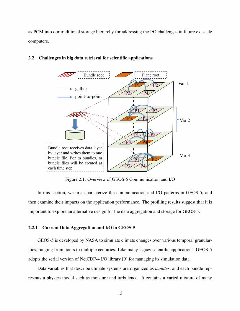
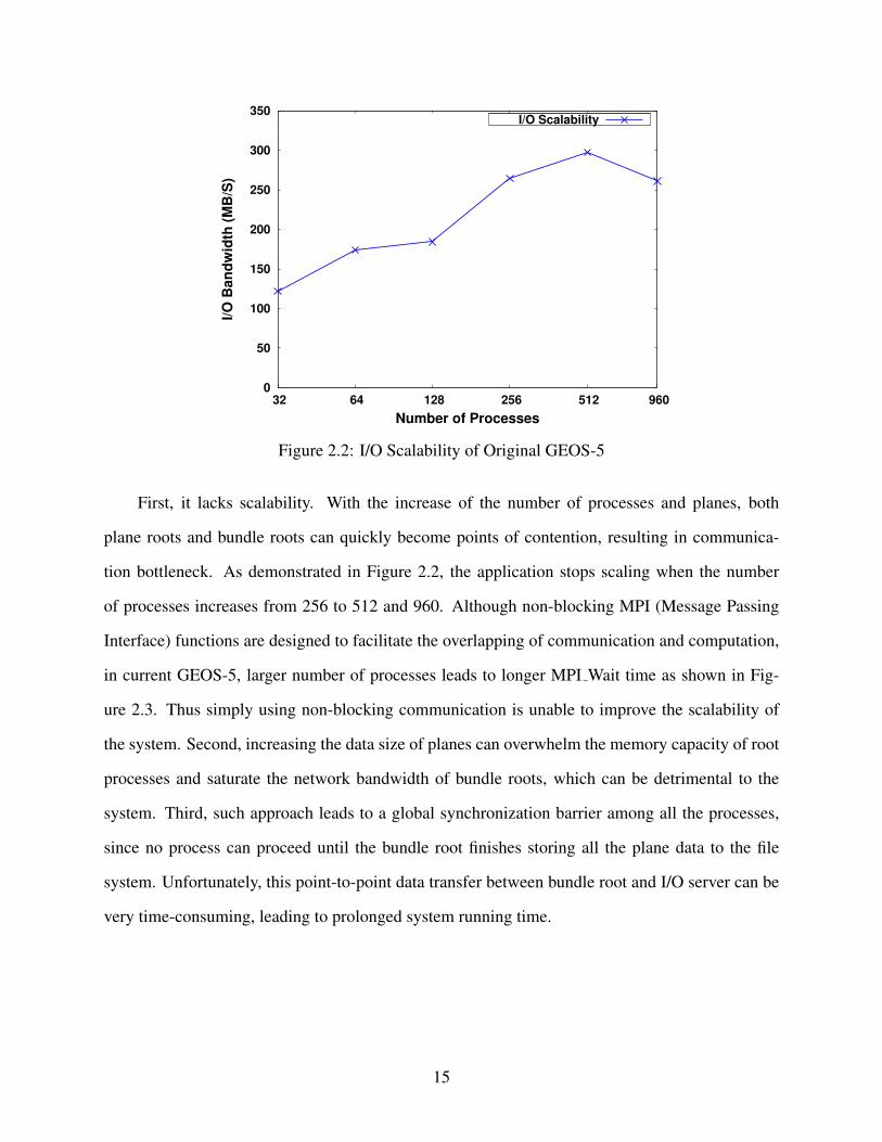
Figure 2.2: I/O Scalability of Original GEOS-5
First, it lacks scalability. With the increase of the number of processes and planes, both
plane roots and bundle roots can quickly become points of contention, resulting in communica-
tion bottleneck. As demonstrated in Figure 2.2, the application stops scaling when the number
of processes increases from 256 to 512 and 960. Although non-blocking MPI (Message Passing
Interface) functions are designed to facilitate the overlapping of communication and computation,
in current GEOS-5, larger number of processes leads to longer MPI Wait time as shown in Fig-
ure 2.3. Thus simply using non-blocking communication is unable to improve the scalability of
the system. Second, increasing the data size of planes can overwhelm the memory capacity of root
processes and saturate the network bandwidth of bundle roots, which can be detrimental to the
system. Third, such approach leads to a global synchronization barrier among all the processes,
since no process can proceed until the bundle root finishes storing all the plane data to the file
system. Unfortunately, this point-to-point data transfer between bundle root and I/O server can be
very time-consuming, leading to prolonged system running time.
15
0
2
4
6
8
10
32 64 128 256 512
Tota
l His
tory
I/O
Tim
e (
sec)
Number of Processes
7 Bundles Time dissection
create post wait
Figure 2.3: Time Dissection of Non-blocking MPI Communication
0
5
10
15
20
25
prog surf bud moist gwd turb tend
Time (sec)
Bundle Name
other 6me
bundle write
bundle comm
layer comm
Figure 2.4: Time Dissection for Collecting and Storing Bundles
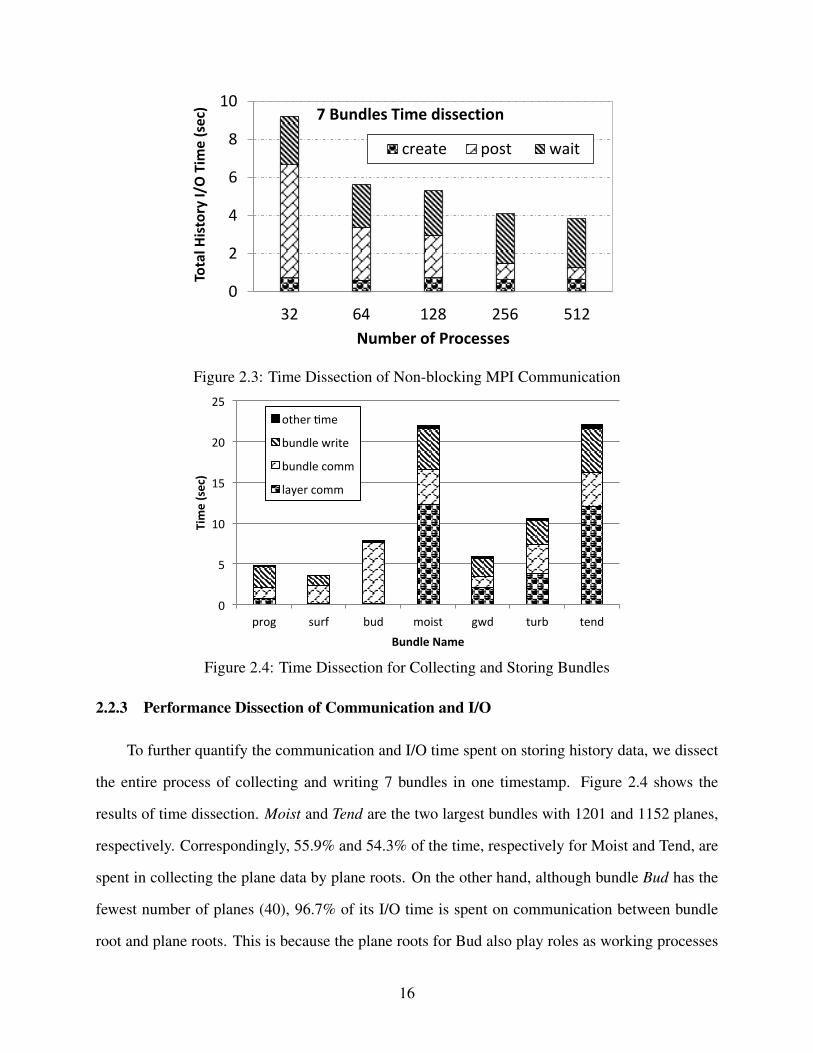
2.2.3 Performance Dissection of Communication and I/O
To further quantify the communication and I/O time spent on storing history data, we dissect
the entire process of collecting and writing 7 bundles in one timestamp. Figure 2.4 shows the
results of time dissection. Moist and Tend are the two largest bundles with 1201 and 1152 planes,
respectively. Correspondingly, 55.9% and 54.3% of the time, respectively for Moist and Tend, are
spent in collecting the plane data by plane roots. On the other hand, although bundle Bud has the
fewest number of planes (40), 96.7% of its I/O time is spent on communication between bundle
root and plane roots. This is because the plane roots for Bud also play roles as working processes
16
for other bundles. This delays the progress of plane data collection for the bundle Bud. In addition,
on average, the I/O time for writing the bundle into the file system only consumes about 27% of
total time of writing the history data.
Gathering data consumes a significant portion of I/O time for the history data as shown in
Figure 2.4. Such implementation limits the scalability and is incapable of supporting large datasets.
Many parallel I/O techniques are viable to address this issue; however, the hierarchical I/O scheme
depicted in Figure 2.1 is unable to leverage these techniques. Therefore, it is critical to overhaul
the architecture of scientific application so that it can efficiently run on large-scale cluster with
hundreds of thousands of processing cores.
2.3 Performance and Fairness Issues Caused by Semantic Unawareness
In this section, we elaborate the performance and unfairness issues for concurrent queries due
to the lack of semantic awareness in the current Hive/Hadoop framework.
2.3.1 Execution Stalls of Concurrent Queries
TPC-H [13] represents a popular online analytical workload. We have conducted a test using
a mixture of three TPC-H queries: two instances of Q14 and one of Q17. Q14 evaluates the market
response to a production promotion in one month. Q17 determines the loss of average yearly
revenue if some orders are not properly fulfilled in time. For convenient description, we name
them as QA and QC for the two instances of Q14 and QB for Q17, respectively. Figure 2.5 shows
the DAGs for three queries and their constituent jobs. QA and QC are small queries with two short
jobs: Aggregate (AGG) and Sort. QB is a large query with four jobs.
In our experiment, we submit QA, QB and QC one after another to our Hadoop cluster. We
profile the use of map and reduce slots along with the progress of queries. Figure 2.6 shows the
results with the HCS scheduler. J1 and J2 from QB arrive before QA-J2 and QC-J2. They are
scheduled for execution, as a result, blocking QA-J2 and QC-J2 from getting map and reduce
slots. We can observe that QA-J2 and QC-J2 both experience execution stalls due to the lack of
17
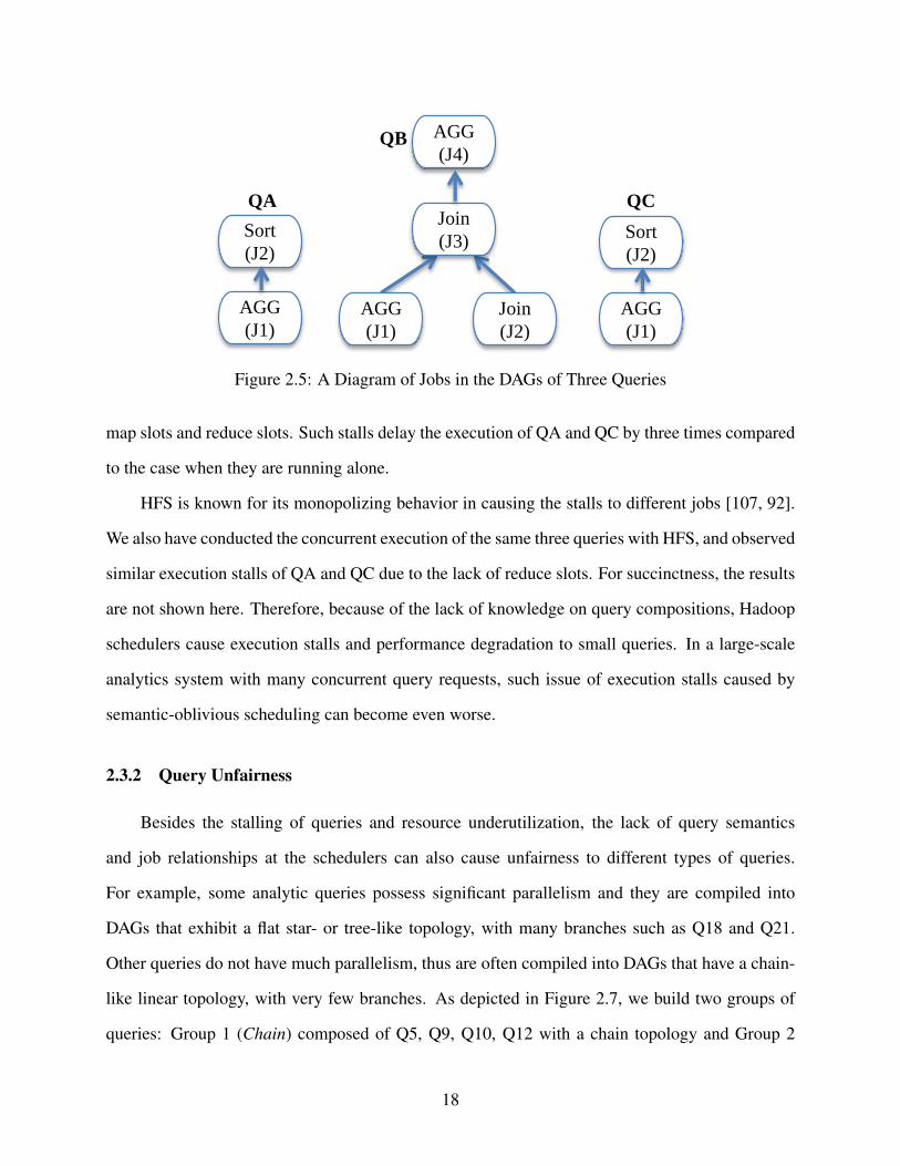
AGG
(J1)
Join
(J3)
Join
(J2)
AGG
(J4)
AGG
(J1)
Sort
(J2)
QB
QC
AGG
(J1)
Sort
(J2)
QA
Figure 2.5: A Diagram of Jobs in the DAGs of Three Queries
map slots and reduce slots. Such stalls delay the execution of QA and QC by three times compared
to the case when they are running alone.
HFS is known for its monopolizing behavior in causing the stalls to different jobs [107, 92].
We also have conducted the concurrent execution of the same three queries with HFS, and observed
similar execution stalls of QA and QC due to the lack of reduce slots. For succinctness, the results
are not shown here. Therefore, because of the lack of knowledge on query compositions, Hadoop
schedulers cause execution stalls and performance degradation to small queries. In a large-scale
analytics system with many concurrent query requests, such issue of execution stalls caused by
semantic-oblivious scheduling can become even worse.
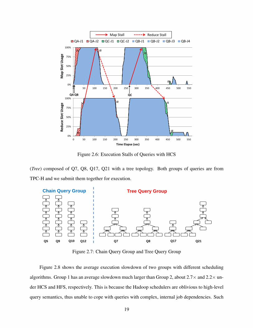
2.3.2 Query Unfairness
Besides the stalling of queries and resource underutilization, the lack of query semantics
and job relationships at the schedulers can also cause unfairness to different types of queries.
For example, some analytic queries possess significant parallelism and they are compiled into
DAGs that exhibit a flat star- or tree-like topology, with many branches such as Q18 and Q21.
Other queries do not have much parallelism, thus are often compiled into DAGs that have a chain-
like linear topology, with very few branches. As depicted in Figure 2.7, we build two groups of
queries: Group 1 (Chain) composed of Q5, Q9, Q10, Q12 with a chain topology and Group 2
18
0%
25%
50%
75%
100%
0 50 100 150 200 250 300 350 400 450 500 550
Re
du
ce S
lot
Usa
ge
0%
25%
50%
75%
100%
0 50 100 150 200 250 300 350 400 450 500 550
Map
Slo
t U
sage
QA-J1 QA-J2 QC-J1 QC-J2 QB-J1 QB-J2 QB-J3 QB-J4
QA QB QC
Map Stall Reduce Stall
J1
J1
J2
J2
J1
J1
J2
J2
Time Elapse (sec)
Figure 2.6: Execution Stalls of Queries with HCS
(Tree) composed of Q7, Q8, Q17, Q21 with a tree topology. Both groups of queries are from
TPC-H and we submit them together for execution.
Q5 Q9 Q10 Q12 Q7 Q8 Q17 Q21
Chain Query Group Tree Query Group
Figure 2.7: Chain Query Group and Tree Query Group
Figure 2.8 shows the average execution slowdown of two groups with different scheduling
algorithms. Group 1 has an average slowdown much larger than Group 2, about 2.7× and 2.2× un-
der HCS and HFS, respectively. This is because the Hadoop schedulers are oblivious to high-level
query semantics, thus unable to cope with queries with complex, internal job dependencies. Such
19
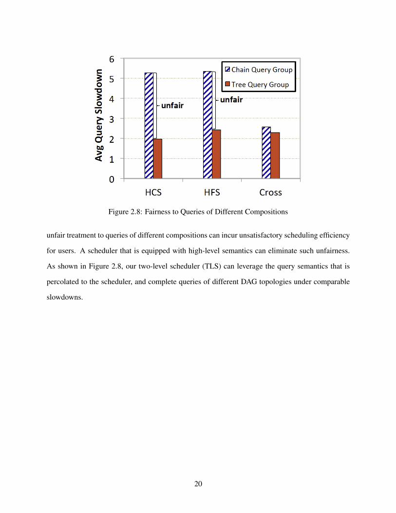
Figure 2.8: Fairness to Queries of Different Compositions
unfair treatment to queries of different compositions can incur unsatisfactory scheduling efficiency
for users. A scheduler that is equipped with high-level semantics can eliminate such unfairness.
As shown in Figure 2.8, our two-level scheduler (TLS) can leverage the query semantics that is
percolated to the scheduler, and complete queries of different DAG topologies under comparable
slowdowns.
20
Chapter 3
PCM Based Hybrid Storage
3.1 Design for PCM Based Hybrid Storage
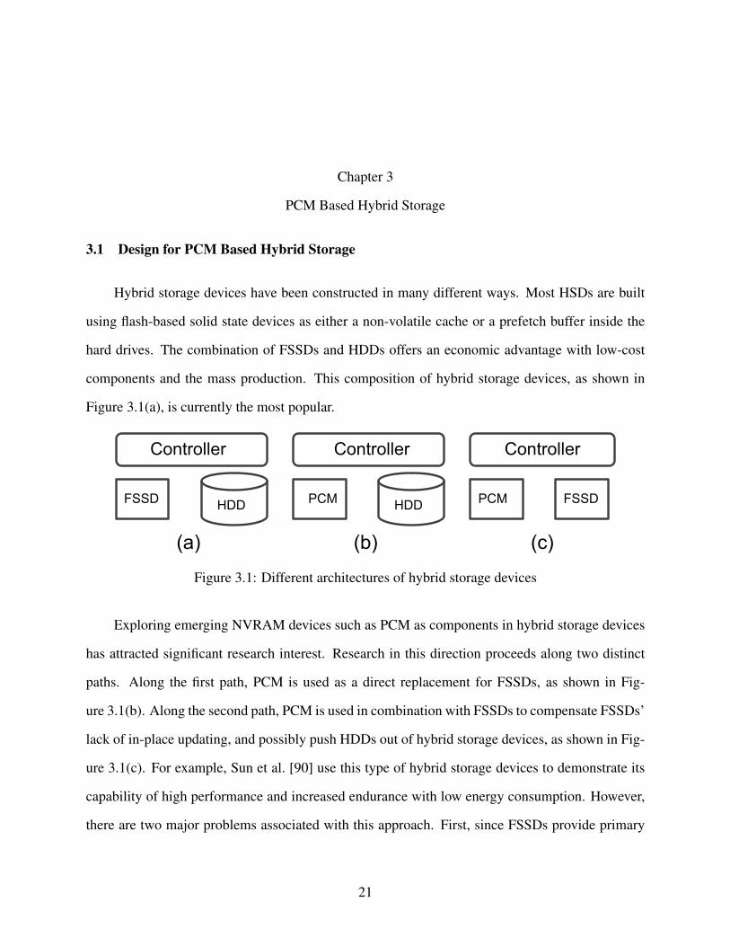
Hybrid storage devices have been constructed in many different ways. Most HSDs are built
using flash-based solid state devices as either a non-volatile cache or a prefetch buffer inside the
hard drives. The combination of FSSDs and HDDs offers an economic advantage with low-cost
components and the mass production. This composition of hybrid storage devices, as shown in
Figure 3.1(a), is currently the most popular.
HDD FSSD
Controller
PCM FSSD
Controller
HDD PCM
Controller
(a) (b) (c)
Figure 3.1: Different architectures of hybrid storage devices
Exploring emerging NVRAM devices such as PCM as components in hybrid storage devices
has attracted significant research interest. Research in this direction proceeds along two distinct
paths. Along the first path, PCM is used as a direct replacement for FSSDs, as shown in Fig-
ure 3.1(b). Along the second path, PCM is used in combination with FSSDs to compensate FSSDs’
lack of in-place updating, and possibly push HDDs out of hybrid storage devices, as shown in Fig-
ure 3.1(c). For example, Sun et al. [90] use this type of hybrid storage devices to demonstrate its
capability of high performance and increased endurance with low energy consumption. However,
there are two major problems associated with this approach. First, since FSSDs provide primary
21
data storage space, the erasure-before-write problem still exists, although it happens at lower fre-
quency. This causes significant performance loss for data intensive applications. Second, without
HDDs in the memory hierarchy, large volumes of storage space cannot be leveraged at reason-
able performance costs. In terms of cost per gigabyte, FSSDs are still about 10 to 20 times more
expensive than HDDs.
For the above reasons, we investigate the benefits of leveraging PCM as a write cache for hy-
brid storage devices that are designed along the first path. As shown in Figure 3.1(b), we use PCMs
to completely replace FSSDs while retaining HDDs for their advantages in storage capacity. With
the fast development of PCM technologies, we expect that the PCM-based hybrid storage drive
will become more popular. In this section, we describe our hybrid storage system - HALO that
uses PCM in a write cache for HDDs to improve performance and reliability of HDD-based stor-
age and file systems. Specifically, we first introduce the HALO framework and its basic supportive
data structures, and then elaborate on the caching and destaging algorithms.
3.1.1 HALO Framework and Data Structures
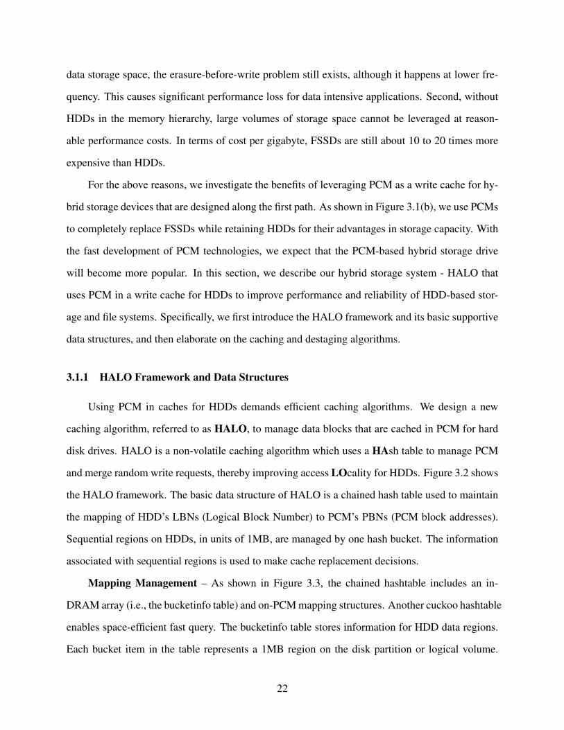
Using PCM in caches for HDDs demands efficient caching algorithms. We design a new
caching algorithm, referred to as HALO, to manage data blocks that are cached in PCM for hard
disk drives. HALO is a non-volatile caching algorithm which uses a HAsh table to manage PCM
and merge random write requests, thereby improving access LOcality for HDDs. Figure 3.2 shows
the HALO framework. The basic data structure of HALO is a chained hash table used to maintain
the mapping of HDD’s LBNs (Logical Block Number) to PCM’s PBNs (PCM block addresses).
Sequential regions on HDDs, in units of 1MB, are managed by one hash bucket. The information
associated with sequential regions is used to make cache replacement decisions.
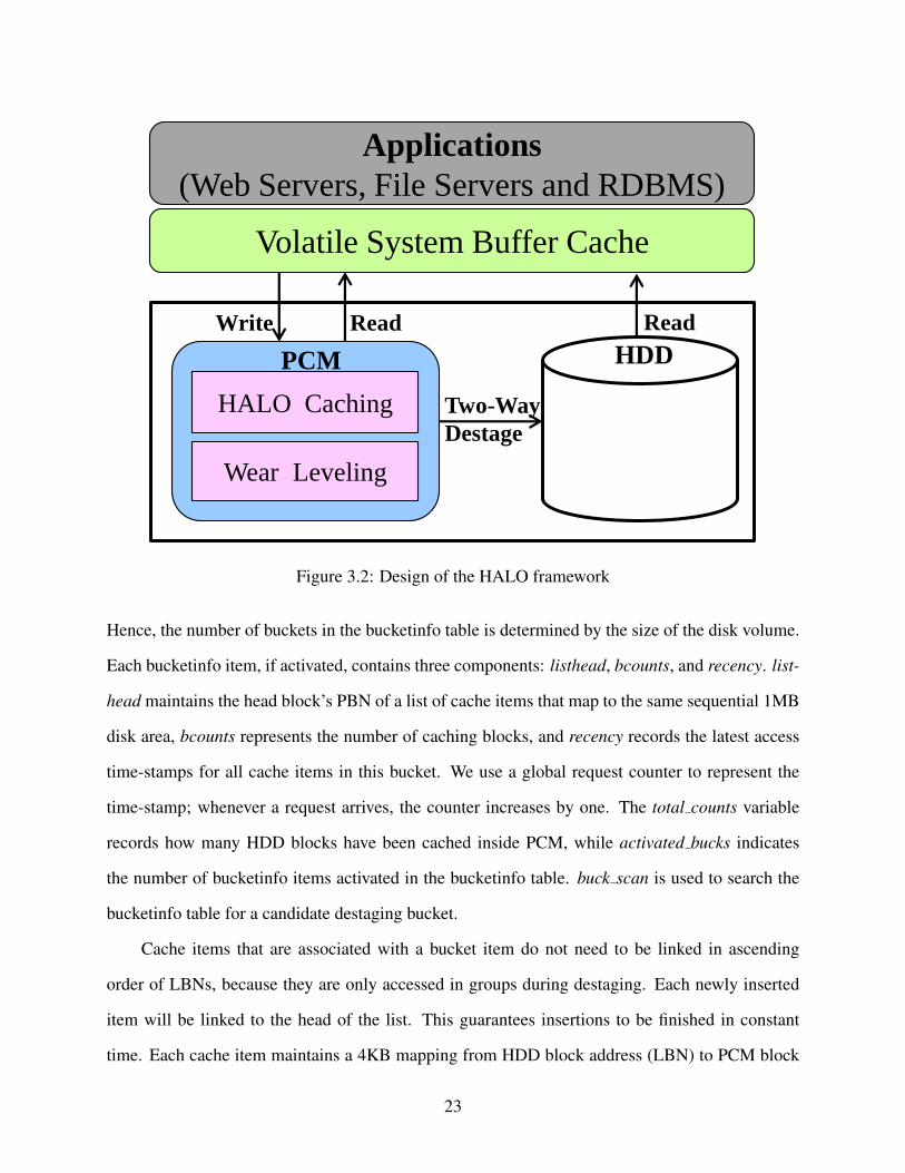
Mapping Management – As shown in Figure 3.3, the chained hashtable includes an in-
DRAM array (i.e., the bucketinfo table) and on-PCM mapping structures. Another cuckoo hashtable
enables space-efficient fast query. The bucketinfo table stores information for HDD data regions.
Each bucket item in the table represents a 1MB region on the disk partition or logical volume.
22
HALO Caching
Wear Leveling
Volatile System Buffer Cache
PCM HDD
Applications
(Web Servers, File Servers and RDBMS)
Two-Way
Destage
Read Write Read
Figure 3.2: Design of the HALO framework
Hence, the number of buckets in the bucketinfo table is determined by the size of the disk volume.
Each bucketinfo item, if activated, contains three components: listhead, bcounts, and recency. list-
head maintains the head block’s PBN of a list of cache items that map to the same sequential 1MB
disk area, bcounts represents the number of caching blocks, and recency records the latest access
time-stamps for all cache items in this bucket. We use a global request counter to represent the
time-stamp; whenever a request arrives, the counter increases by one. The total counts variable
records how many HDD blocks have been cached inside PCM, while activated bucks indicates
the number of bucketinfo items activated in the bucketinfo table. buck scan is used to search the
bucketinfo table for a candidate destaging bucket.
Cache items that are associated with a bucket item do not need to be linked in ascending
order of LBNs, because they are only accessed in groups during destaging. Each newly inserted
item will be linked to the head of the list. This guarantees insertions to be finished in constant
time. Each cache item maintains a 4KB mapping from HDD block address (LBN) to PCM block
23
LBN PBN LBN: x h2(x)
h3(x)
Cache Block
Next PBN
Bitmap LBN
Cache Block
Next PBN
Bitmap LBN
Cache Block
Next PBN
Bitmap LBN
Bucket[i] Listhead Recency Bcounts
Buckinfo_table
DRAM
PCM
… … …
buck_scan
Bucket[0]
Bucket[n] (Empty)
Cuckoo Hashtable
…
…
…
Head
Tail
h1(x)
h4(x)
Cache Item
Figure 3.3: Data structures of HALO caching
number (PBN). It contains a LBN (the starting LBN of 8 sequential HDD blocks), the PBN of the
next PCM block in the list and an 8-bit bitmap which represents the fragmentation inside a 4KB
PCM block. If the 8-bit bitmap is nonzero, the nonzero bits represent cached 512B HDD blocks.
Each cache item is stored on each PCM block’s meta data section [18].
Cuckoo Hash Table – To achieve fast retrieval of HDD blocks, a DRAM-based cuckoo hash
table is maintained using the LBN as the key and the PBN as the value. On a cache hit, the PBN of
the cache item is returned, which enables fast access of data information in the PCM. Traditionally,
hash tables resolve collisions through linear probing or chained hash and they can answer lookup
queries within O(1) time when their load factors are very low, i.e., smaller than log(n)/n, where
n is the table size. With an increasing load factor, its query time can degrade to O(log(n)) or even
O(n). Cuckoo hashing solves the issue by using multiple hash functions [74, 36]. It can achieve
fast lookups within O(1) time (albeit a bigger constant than linear hashing), as well as good space
efficiency i.e. high load factor. Next, we introduce how we achieve such space efficiency.
24
0.5
0.6
0.7
0.8
0.9
1
2 3 4 5 6 7 8
Ma
x L
oa
d F
ac
tor
Num of Hash Functions
Figure 3.4: Max Load Factors for Different Numbers of Hash Functions
We set 100 as the maximum displacement threshold in the Cuckoo hashtable. When the
Cuckoo hashtable cannot find an available slot for a new inserting record within 100 item displace-
ments, it indicates that the hashtable is almost full and requires a larger size table and rehashing.
And such critical load factor before rehashing is counted as maximum load factor. Figure 3.4 shows
how the number of hash functions influences the average maximum load factor we can achieve for
running seven traces above. When the number of functions is two, only 50% load factor can be
achieved; as the number of functions increases, the load factor of Cuckoo hash tables initially
grows rapidly and then the slope of the curve becomes smaller thus the benefit achieved becomes
marginal. Therefore we use four functions in our design since a larger number of functions can
in turn bring higher query and computation overheads. In addition, we set a larger initial size of
hashtable to keep the load factor lower than 80% percent when PCM cache is fully loaded. In this
way we are able to maintain the average displacements per insert below 2 for better performance.
25
Here, we give a sample calculation of DRAM overhead by the HALO data structures. In total,
for a 2 GB PCM cache with 4 KB cache block size, 0.5 M items will placed be in the hashtable.
As each item takes 8 Bytes and the load factor of the cuckoo hashtable is 0.8, the total memory
overhead of the Cuckoo hashtable is about 5 MB. With the bucketinfo table normally consuming
about 6-12 MB DRAM, we need less than 20 MB DRAM to implement HALO cache management
for 2 GB PCM and 1 TB hard disk.
Recovery from System Crashes – Mapping information of a PCM block that contains the
LBN, the next PBN and the bitmap are stored on non-volatile PCM. Therefore, in case the system
crashes, it can first reboot and then either destage the dirty items from PCM to HDD or rebuild the
in-DRAM hashtables by scanning information on fixed positions of the PCM meta data sections
(to get the cache items’ information including LBN, bitmap and next PBN). As the PCM’s read
performance is similar to that of DRAM, the recovery procedure should only take seconds to
rebuild the in-memory mapping data structures. In doing so, we can avoid loss of cached data and
guarantee the system integrity.
3.1.2 HALO Caching Scheme
Our caching algorithm is described in Algorithm 1. When a request arrives, the bucket index
is computed using the request’s LBN. The hash table is then searched for an entry corresponding
to the LBN. In the event of a cache hit, the PBNs are returned from the hash table and the corre-
sponding blocks are either written in-place to, or read from, the PCM. The corresponding bucket’s
recency in the bucketinfo table is also updated to the current time-stamp. In the event of a cache
miss on a read request, data is read directly from the HDD without updating the cache. In the event
of a cache miss on a write request, a cache item is allocated in the PCM, and data is written to
that cache block. Then, if the bucket item of the bucketinfo table for the LBN is empty, it will be
activated. After that, the bucket item’s list of cache items is updated, the address mapping informa-
tion is added to the hash table, the recency of this bucket is set to the current time-stamp, and the
26
bucket’s bcounts is incremented. The updated access statistic information are used by the two-way
destaging algorithm to conduct destaging procedures.
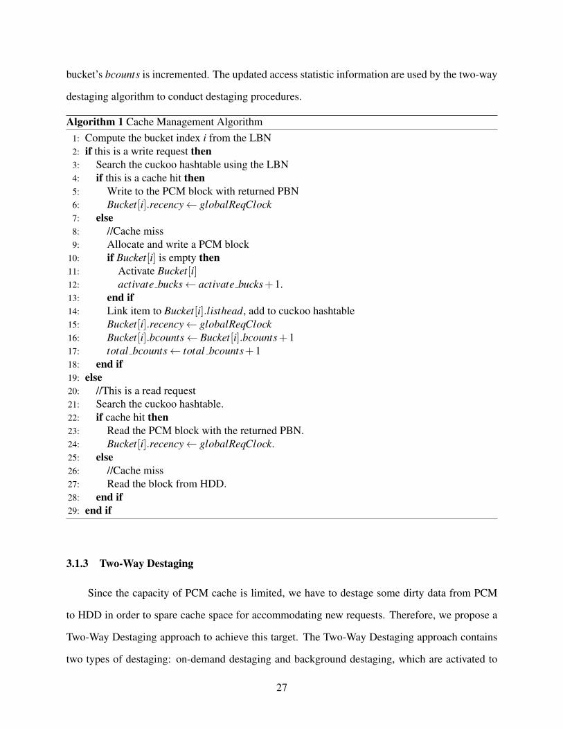
Algorithm 1 Cache Management Algorithm1: Compute the bucket index i from the LBN2: if this is a write request then3: Search the cuckoo hashtable using the LBN4: if this is a cache hit then5: Write to the PCM block with returned PBN6: Bucket[i].recency← globalReqClock7: else8: //Cache miss9: Allocate and write a PCM block
10: if Bucket[i] is empty then11: Activate Bucket[i]12: activate bucks← activate bucks+1.13: end if14: Link item to Bucket[i].listhead, add to cuckoo hashtable15: Bucket[i].recency← globalReqClock16: Bucket[i].bcounts← Bucket[i].bcounts+117: total bcounts← total bcounts+118: end if19: else20: //This is a read request21: Search the cuckoo hashtable.22: if cache hit then23: Read the PCM block with the returned PBN.24: Bucket[i].recency← globalReqClock.25: else26: //Cache miss27: Read the block from HDD.28: end if29: end if
3.1.3 Two-Way Destaging
Since the capacity of PCM cache is limited, we have to destage some dirty data from PCM
to HDD in order to spare cache space for accommodating new requests. Therefore, we propose a
Two-Way Destaging approach to achieve this target. The Two-Way Destaging approach contains
two types of destaging: on-demand destaging and background destaging, which are activated to
27
evict some data buckets out of PCM. Next, we will introduce when to trigger each destaging and
how to select the victim buckets.
The on-demand destaging is activated when the utilization of PCM cache reaches a high
percentage, e.g., 95% of the total size. Such on-demand method can sometimes incur additional
wait delay to front-end I/O requests, especially when the I/O load intensity is high. To complement
this approach and relax such contention, we introduce another destaging method which is triggered
when both the PCM utilization is relatively high, e.g., 80%, and the front-end I/O intensity is low
(specifically, disk performance utilization smaller than 10%). Through combination of these ways
of destaging, PCM space can be appropriately reclaimed with minimal performance impacts to
front-end workloads.
For either destaging method, a bucket is eligible to be destaged to HDDs if any of the follow-
ing two conditions holds: First, the bucket’s bcounts needs to be greater than the average value of
bcounts plus a constant threshold T HBCOUNT S and the bucket’s recency needs to be older than the
global request timestamp by a constant T HRECENCY . For every unsuccessful round of scan, these
two thresholds will dynamically decrease to make sure that victim buckets can be found within a
reasonable number of steps. Second, the bucket’s recency needs to be older than the global request
timestamp by a constant ODRECENCY (ODRECENCY � T HRECENCY ). As soon as a bucket is identi-
fied as eligible for destaging, all cache blocks associated with the bucket are destaged to the HDD
in a batching manner, the bucket is deactivated and the corresponding items in the cuckoo hash
table are deleted. As these cache blocks are mapped to 1MB sequential region of HDD, this batch
of write-backs are supposed to only incur one single seek operation to HDD, thus providing good
write locality and causing minimal affects to read requests.
We select these two criteria for determining destaging candidates for the following reasons.
First, we want to choose a bucket that has enough items to form a large enough sequential write
to the HDD to increase spatial locality of write operations, and at the same time it needs to be one
that is not recently used in order to preserve temporal locality. Second, for those very old and small
buckets, we evict them from the PCM by setting the control variable ODRECENCY .
28
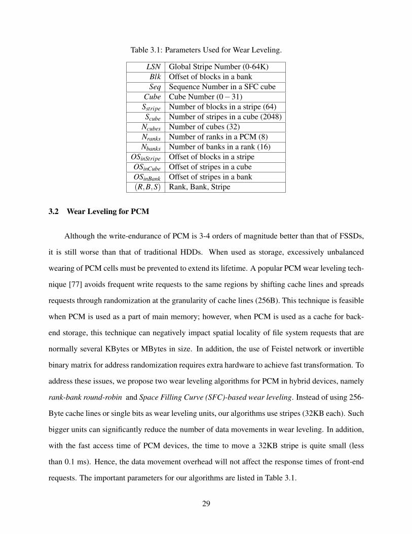
Table 3.1: Parameters Used for Wear Leveling.
LSN Global Stripe Number (0-64K)Blk Offset of blocks in a bankSeq Sequence Number in a SFC cube
Cube Cube Number (0−31)Sstripe Number of blocks in a stripe (64)Scube Number of stripes in a cube (2048)
Ncubes Number of cubes (32)Nranks Number of ranks in a PCM (8)Nbanks Number of banks in a rank (16)
OSinStripe Offset of blocks in a stripeOSinCube Offset of stripes in a cubeOSinBank Offset of stripes in a bank(R,B,S) Rank, Bank, Stripe
3.2 Wear Leveling for PCM
Although the write-endurance of PCM is 3-4 orders of magnitude better than that of FSSDs,
it is still worse than that of traditional HDDs. When used as storage, excessively unbalanced
wearing of PCM cells must be prevented to extend its lifetime. A popular PCM wear leveling tech-
nique [77] avoids frequent write requests to the same regions by shifting cache lines and spreads
requests through randomization at the granularity of cache lines (256B). This technique is feasible
when PCM is used as a part of main memory; however, when PCM is used as a cache for back-
end storage, this technique can negatively impact spatial locality of file system requests that are
normally several KBytes or MBytes in size. In addition, the use of Feistel network or invertible
binary matrix for address randomization requires extra hardware to achieve fast transformation. To
address these issues, we propose two wear leveling algorithms for PCM in hybrid devices, namely
rank-bank round-robin and Space Filling Curve (SFC)-based wear leveling. Instead of using 256-
Byte cache lines or single bits as wear leveling units, our algorithms use stripes (32KB each). Such
bigger units can significantly reduce the number of data movements in wear leveling. In addition,
with the fast access time of PCM devices, the time to move a 32KB stripe is quite small (less
than 0.1 ms). Hence, the data movement overhead will not affect the response times of front-end
requests. The important parameters for our algorithms are listed in Table 3.1.
29
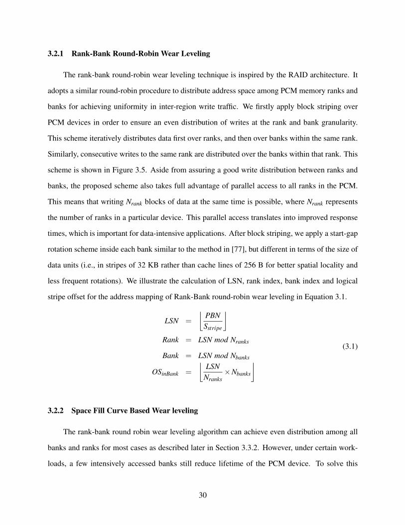
3.2.1 Rank-Bank Round-Robin Wear Leveling
The rank-bank round-robin wear leveling technique is inspired by the RAID architecture. It
adopts a similar round-robin procedure to distribute address space among PCM memory ranks and
banks for achieving uniformity in inter-region write traffic. We firstly apply block striping over
PCM devices in order to ensure an even distribution of writes at the rank and bank granularity.
This scheme iteratively distributes data first over ranks, and then over banks within the same rank.
Similarly, consecutive writes to the same rank are distributed over the banks within that rank. This
scheme is shown in Figure 3.5. Aside from assuring a good write distribution between ranks and
banks, the proposed scheme also takes full advantage of parallel access to all ranks in the PCM.
This means that writing Nrank blocks of data at the same time is possible, where Nrank represents
the number of ranks in a particular device. This parallel access translates into improved response
times, which is important for data-intensive applications. After block striping, we apply a start-gap
rotation scheme inside each bank similar to the method in [77], but different in terms of the size of
data units (i.e., in stripes of 32 KB rather than cache lines of 256 B for better spatial locality and
less frequent rotations). We illustrate the calculation of LSN, rank index, bank index and logical
stripe offset for the address mapping of Rank-Bank round-robin wear leveling in Equation 3.1.
LSN =
⌊PBNSstripe
⌋Rank = LSN mod Nranks
Bank = LSN mod Nbanks
OSinBank =
⌊LSN
Nranks×Nbanks
⌋ (3.1)
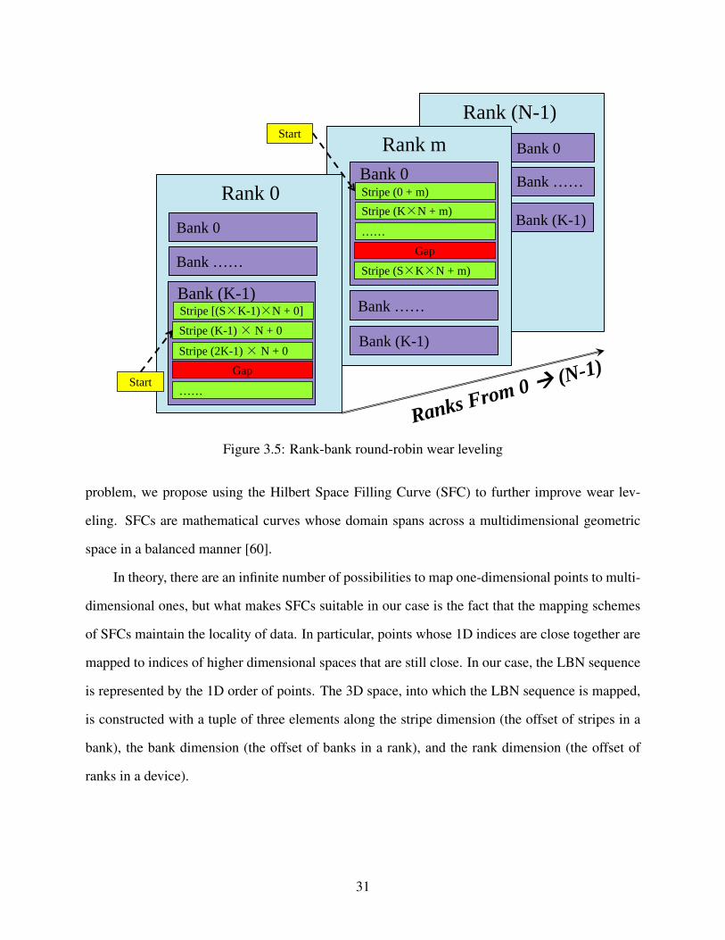
3.2.2 Space Fill Curve Based Wear leveling
The rank-bank round robin wear leveling algorithm can achieve even distribution among all
banks and ranks for most cases as described later in Section 3.3.2. However, under certain work-
loads, a few intensively accessed banks still reduce lifetime of the PCM device. To solve this
30
Rank (N-1)
Bank 0
Bank ……
Bank (K-1)
Rank mBank 0
Stripe (K×N + m)Stripe (0 + m)
……
Stripe (S×K×N + m)
Start
Gap
Bank ……
Bank (K-1)
Rank 0
Bank (K-1)
Stripe (K-1) × N + 0
……
Stripe (2K-1) × N + 0
StartGap
Bank ……
Bank 0
Ranks From 0 (N-1)
Stripe [(S×K-1)×N + 0]
Figure 3.5: Rank-bank round-robin wear leveling
problem, we propose using the Hilbert Space Filling Curve (SFC) to further improve wear lev-
eling. SFCs are mathematical curves whose domain spans across a multidimensional geometric
space in a balanced manner [60].
In theory, there are an infinite number of possibilities to map one-dimensional points to multi-
dimensional ones, but what makes SFCs suitable in our case is the fact that the mapping schemes
of SFCs maintain the locality of data. In particular, points whose 1D indices are close together are
mapped to indices of higher dimensional spaces that are still close. In our case, the LBN sequence
is represented by the 1D order of points. The 3D space, into which the LBN sequence is mapped,
is constructed with a tuple of three elements along the stripe dimension (the offset of stripes in a
bank), the bank dimension (the offset of banks in a rank), and the rank dimension (the offset of
ranks in a device).
31
8
32*16
16Cube 0
Cube 31
R
S
B
0Figure 3.6: Space filling curve based wear leveling
LSN =
⌊PBNSstripe
⌋OSinStripe = PBN mod Sstripe
Cubeno = Stripe mod Ncubes
OSinCube =
⌊StripeNcubes
⌋Seq = StartGapMap(OSinCube)
(R,B,S) = SFCMapFunc(Seq)
(3.2)
We have 512 stripes in a bank, 16 banks in a rank and 8 ranks in a device. We evenly split the
3D space into 32 cubes along the stripe dimension. In other words, the number of stripes in each
cube is 16 × 16 × 8 (i.e., #stripe × #bank × #rank). After splitting, we apply the round-robin
method to distribute accesses across these cubes. And inside every cube, a start-gap like stripe
shifting is implemented, making the 3D SFC cube move like a snake. The consequence is that
32
consecutive writes in the same cube can only happen for addresses that are 32 stripes away, which
dramatically reduces the possibility of intensive writing in the same region. Within each cube, we
apply SFC to further disperse accesses. We orchestrate SFC to disperse accesses across ranks as
much as possible. This helps exploit parallelism from the hardware.
In summary, using SFC in combination with the round-robin method, we are able to map a
1D sequence of block numbers into a 3D triple of stripe number, rank number and bank number.
The address mapping scheme is generally depicted in Figure 3.6. The left figure shows the logical
organization of the device with its 32 cubes (or parallelepiped’s, to be more precise, because the
size is 8×16×16). The right figure shows a 3-dimensional space filling curve that is used for our
work. The mapping scheme starts with PBN provided by the system and ends up with a 3-tuple
(R, B, S) calculated based on Equation 3.2. The SFC based wear leveling is designed for a best
trade-off among write uniformity, access parallelism and spatial locality.
3.3 Evaluation for PCM-Based Hybrid Storage
To realize our proposed PCM-based write cache for hybrid storage devices we have designed
a PCM simulation framework that simulates different caching schemes (HALO and LRU), wear
leveling algorithms and PCM devices’ characteristics including hardware structure, performance
and wearing status. The simulators are written in about 4,300 lines of C.
As we can see from Figure 3.7, during evaluation, the block-level I/O traces are input to the
simulators. The I/O requests are then processed by caching and wear leveling schemes, which
generate two types of intermediate I/O requests: PCM requests and HDD requests. The PCM
requests are processed by the PCM simulator to get response and wear leveling results. The HDD
requests come from cache misses and destaging, which are stored as HDD trace files. HDD trace
files are then replayed by the blktrace tool [23] on a 500GB, 7200RPM Seagate disk in a CentOS
5 Linux 2.6.32 system with an Intel E4400 CPU and 2.0 GB memory. The DRAM-based system
buffer cache is bypassed by the HDD trace replaying process. Traces are replayed in a close-loop
way for measuring system service rate.
33
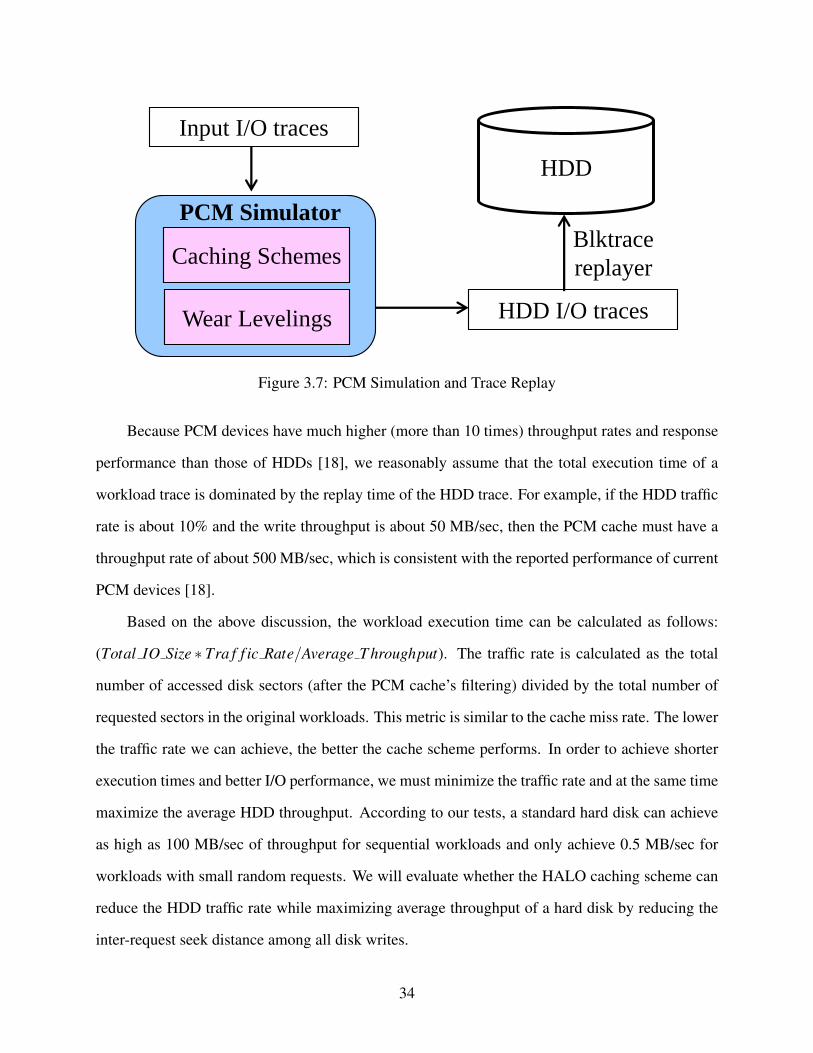
Caching Schemes
HDD
PCM Simulator
Wear Levelings
Input I/O traces
HDD I/O traces
Blktrace
replayer
Figure 3.7: PCM Simulation and Trace Replay
Because PCM devices have much higher (more than 10 times) throughput rates and response
performance than those of HDDs [18], we reasonably assume that the total execution time of a
workload trace is dominated by the replay time of the HDD trace. For example, if the HDD traffic
rate is about 10% and the write throughput is about 50 MB/sec, then the PCM cache must have a
throughput rate of about 500 MB/sec, which is consistent with the reported performance of current
PCM devices [18].
Based on the above discussion, the workload execution time can be calculated as follows:
(Total IO Size ∗ Tra f f ic Rate/Average T hroughput). The traffic rate is calculated as the total
number of accessed disk sectors (after the PCM cache’s filtering) divided by the total number of
requested sectors in the original workloads. This metric is similar to the cache miss rate. The lower
the traffic rate we can achieve, the better the cache scheme performs. In order to achieve shorter
execution times and better I/O performance, we must minimize the traffic rate and at the same time
maximize the average HDD throughput. According to our tests, a standard hard disk can achieve
as high as 100 MB/sec of throughput for sequential workloads and only achieve 0.5 MB/sec for
workloads with small random requests. We will evaluate whether the HALO caching scheme can
reduce the HDD traffic rate while maximizing average throughput of a hard disk by reducing the
inter-request seek distance among all disk writes.
34
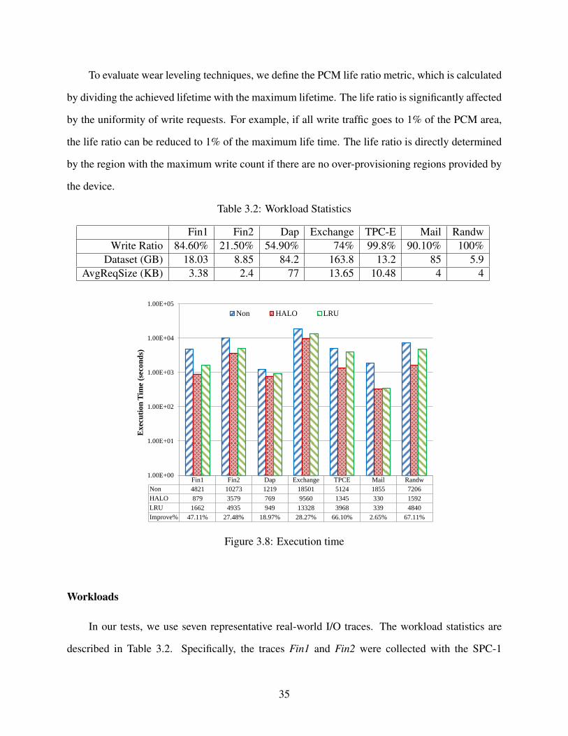
To evaluate wear leveling techniques, we define the PCM life ratio metric, which is calculated
by dividing the achieved lifetime with the maximum lifetime. The life ratio is significantly affected
by the uniformity of write requests. For example, if all write traffic goes to 1% of the PCM area,
the life ratio can be reduced to 1% of the maximum life time. The life ratio is directly determined
by the region with the maximum write count if there are no over-provisioning regions provided by
the device.
Table 3.2: Workload Statistics
Fin1 Fin2 Dap Exchange TPC-E Mail RandwWrite Ratio 84.60% 21.50% 54.90% 74% 99.8% 90.10% 100%
Dataset (GB) 18.03 8.85 84.2 163.8 13.2 85 5.9AvgReqSize (KB) 3.38 2.4 77 13.65 10.48 4 4
Fin1 Fin2 Dap Exchange TPCE Mail Randw
Non 4821 10273 1219 18501 5124 1855 7206
HALO 879 3579 769 9560 1345 330 1592
LRU 1662 4935 949 13328 3968 339 4840
Improve% 47.11% 27.48% 18.97% 28.27% 66.10% 2.65% 67.11%
0
0.1
0.2
0.3
0.4
0.5
0.6
0.7
0.8
1.00E+00
1.00E+01
1.00E+02
1.00E+03
1.00E+04
1.00E+05
Ex
ecu
tio
n T
ime
(sec
on
ds)
Non HALO LRU Improve%
Figure 3.8: Execution time
Workloads
In our tests, we use seven representative real-world I/O traces. The workload statistics are
described in Table 3.2. Specifically, the traces Fin1 and Fin2 were collected with the SPC-1
35
benchmark suite at a large financial organization [14]; the trace Dap was collected at a Display Ad-
vertisement Platform’s payload server; the trace Exchange was collected at a Microsoft Exchange
2007 mail server for 5,000 corporate users; the trace TPC-E was collected on a storage system of
12 28-disk RAID-0 arrays under an OLTP benchmark, TPC-E [15]; the trace Mail was collected
on a mail server by Florida International University [15]. The seventh trace Randw was collected
by us on the target disk while running the IOmeter benchmark with the 4KB-100% random-100%
write workload for 2 hours [73].
Table 3.3: The Effects of Cuckoo Hash Function Numbers on Load Factors
func number 2 3 4 5 6 7 8load factor 0.506082 0.887596 0.956696 0.968351 0.985249 0.988124 0.991324
3.3.1 I/O Performance
0
0.1
0.2
0.3
0.4
0.5
0.6
0.7
0.8
0.9
1
256M 512M 768M 1G 2G 3G 4G 6G
Tra
ffic
Ra
te
PCM cache size (Bytes)
Fin1-HALO
Fin1-LRU
Fin2-HALO
Fin2-LRU
Dap-HALO
Dap-LRU
Figure 3.9: Traffic rate for Fin1, Fin2 and Dap
To evaluate execution times of seven traces, we choose 512MB as the cache size for Fin1 and
Fin2, and 2GB as the cache size for the other five traces. Figure 3.8 shows the results for Non-
cache, HALO-cache and LRU-cache respectively. As we can see, the execution times are reduced
greatly for all traces. The execution improvement of HALO caching over LRU caching is 47.11%
36
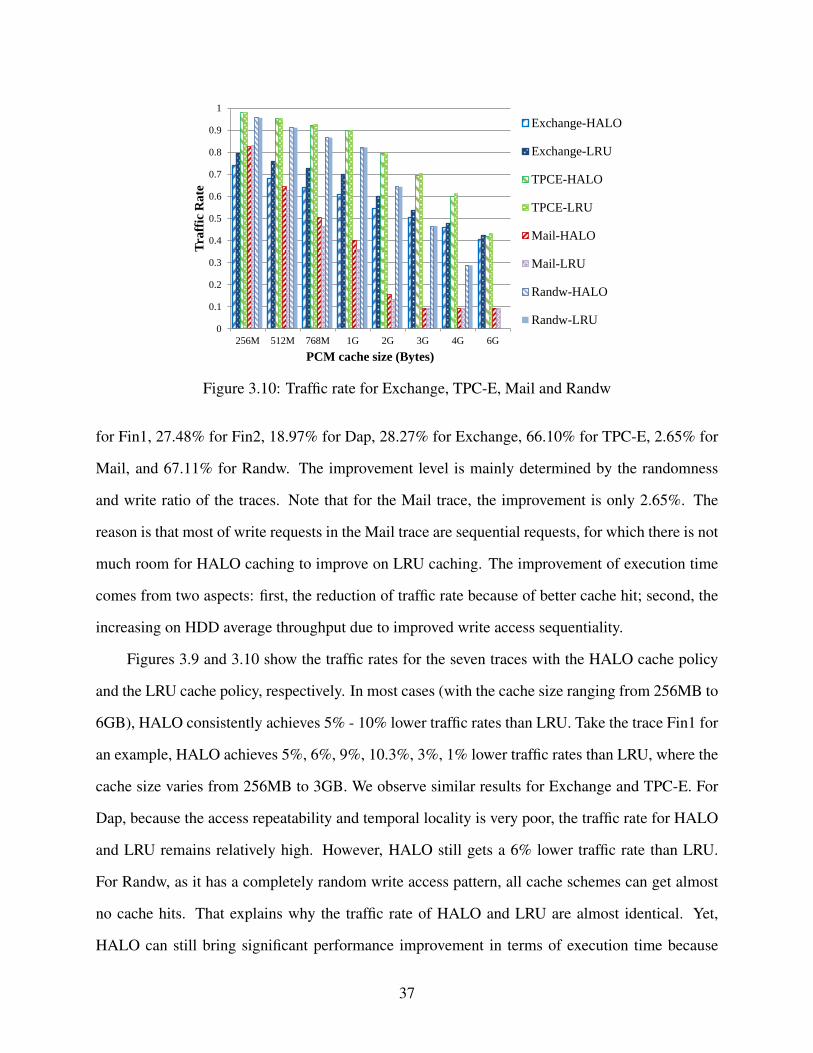
0
0.1
0.2
0.3
0.4
0.5
0.6
0.7
0.8
0.9
1
256M 512M 768M 1G 2G 3G 4G 6G
Tra
ffic
Ra
te
PCM cache size (Bytes)
Exchange-HALO
Exchange-LRU
TPCE-HALO
TPCE-LRU
Mail-HALO
Mail-LRU
Randw-HALO
Randw-LRU
Figure 3.10: Traffic rate for Exchange, TPC-E, Mail and Randw
for Fin1, 27.48% for Fin2, 18.97% for Dap, 28.27% for Exchange, 66.10% for TPC-E, 2.65% for
Mail, and 67.11% for Randw. The improvement level is mainly determined by the randomness
and write ratio of the traces. Note that for the Mail trace, the improvement is only 2.65%. The
reason is that most of write requests in the Mail trace are sequential requests, for which there is not
much room for HALO caching to improve on LRU caching. The improvement of execution time
comes from two aspects: first, the reduction of traffic rate because of better cache hit; second, the
increasing on HDD average throughput due to improved write access sequentiality.
Figures 3.9 and 3.10 show the traffic rates for the seven traces with the HALO cache policy
and the LRU cache policy, respectively. In most cases (with the cache size ranging from 256MB to
6GB), HALO consistently achieves 5% - 10% lower traffic rates than LRU. Take the trace Fin1 for
an example, HALO achieves 5%, 6%, 9%, 10.3%, 3%, 1% lower traffic rates than LRU, where the
cache size varies from 256MB to 3GB. We observe similar results for Exchange and TPC-E. For
Dap, because the access repeatability and temporal locality is very poor, the traffic rate for HALO
and LRU remains relatively high. However, HALO still gets a 6% lower traffic rate than LRU.
For Randw, as it has a completely random write access pattern, all cache schemes can get almost
no cache hits. That explains why the traffic rate of HALO and LRU are almost identical. Yet,
HALO can still bring significant performance improvement in terms of execution time because
37
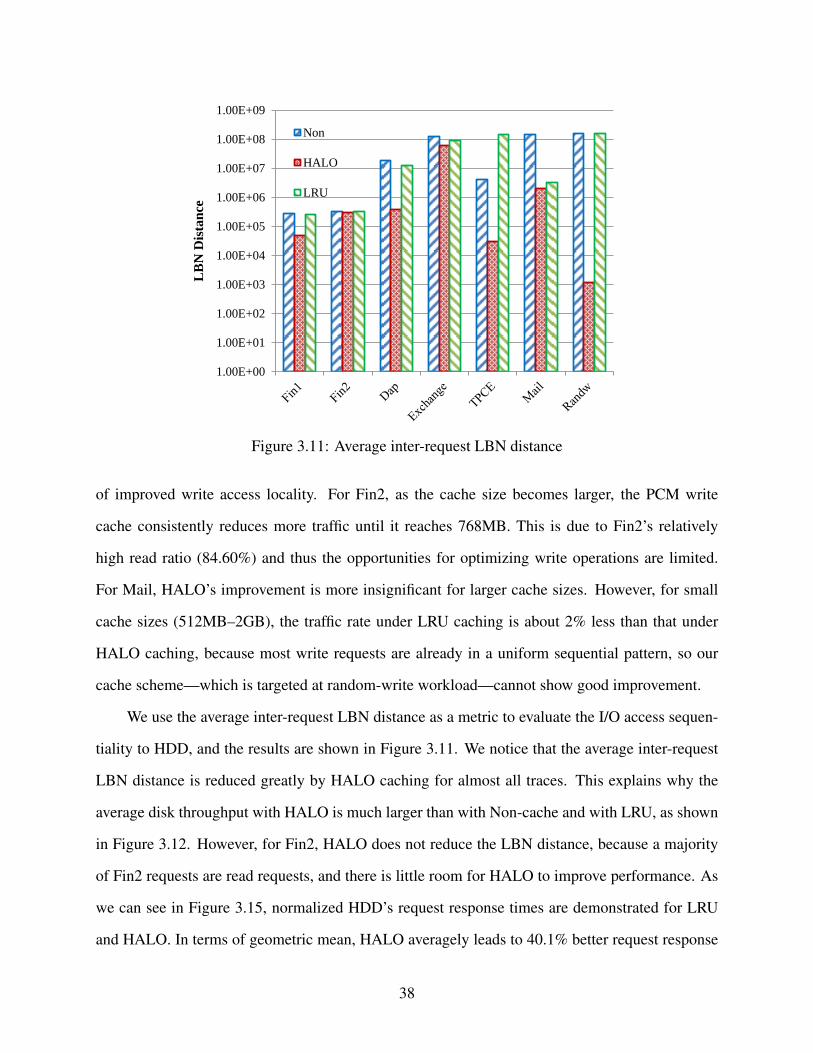
1.00E+00
1.00E+01
1.00E+02
1.00E+03
1.00E+04
1.00E+05
1.00E+06
1.00E+07
1.00E+08
1.00E+09
LB
N D
ista
nce
Non
HALO
LRU
Figure 3.11: Average inter-request LBN distance
of improved write access locality. For Fin2, as the cache size becomes larger, the PCM write
cache consistently reduces more traffic until it reaches 768MB. This is due to Fin2’s relatively
high read ratio (84.60%) and thus the opportunities for optimizing write operations are limited.
For Mail, HALO’s improvement is more insignificant for larger cache sizes. However, for small
cache sizes (512MB–2GB), the traffic rate under LRU caching is about 2% less than that under
HALO caching, because most write requests are already in a uniform sequential pattern, so our
cache scheme—which is targeted at random-write workload—cannot show good improvement.
We use the average inter-request LBN distance as a metric to evaluate the I/O access sequen-
tiality to HDD, and the results are shown in Figure 3.11. We notice that the average inter-request
LBN distance is reduced greatly by HALO caching for almost all traces. This explains why the
average disk throughput with HALO is much larger than with Non-cache and with LRU, as shown
in Figure 3.12. However, for Fin2, HALO does not reduce the LBN distance, because a majority
of Fin2 requests are read requests, and there is little room for HALO to improve performance. As
we can see in Figure 3.15, normalized HDD’s request response times are demonstrated for LRU
and HALO. In terms of geometric mean, HALO averagely leads to 40.1% better request response
38
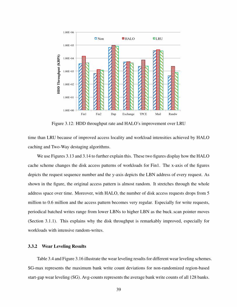
1.00E+00
1.00E+01
1.00E+02
1.00E+03
1.00E+04
1.00E+05
1.00E+06
Fin1 Fin2 Dap Exchange TPCE Mail Randw
HD
D T
hrou
ghpu
t (K
BPS
)
Non HALO LRU
Figure 3.12: HDD throughput rate and HALO’s improvement over LRU
time than LRU because of improved access locality and workload intensities achieved by HALO
caching and Two-Way destaging algorithms.
We use Figures 3.13 and 3.14 to further explain this. These two figures display how the HALO
cache scheme changes the disk access patterns of workloads for Fin1. The x-axis of the figures
depicts the request sequence number and the y-axis depicts the LBN address of every request. As
shown in the figure, the original access pattern is almost random. It stretches through the whole
address space over time. Moreover, with HALO, the number of disk access requests drops from 5
million to 0.6 million and the access pattern becomes very regular. Especially for write requests,
periodical batched writes range from lower LBNs to higher LBN as the buck scan pointer moves
(Section 3.1.1). This explains why the disk throughput is remarkably improved, especially for
workloads with intensive random-writes.
3.3.2 Wear Leveling Results
Table 3.4 and Figure 3.16 illustrate the wear leveling results for different wear leveling schemes.
SG-max represents the maximum bank write count deviations for non-randomized region-based
start-gap wear leveling (SG). Avg-counts represents the average bank write counts of all 128 banks.
39
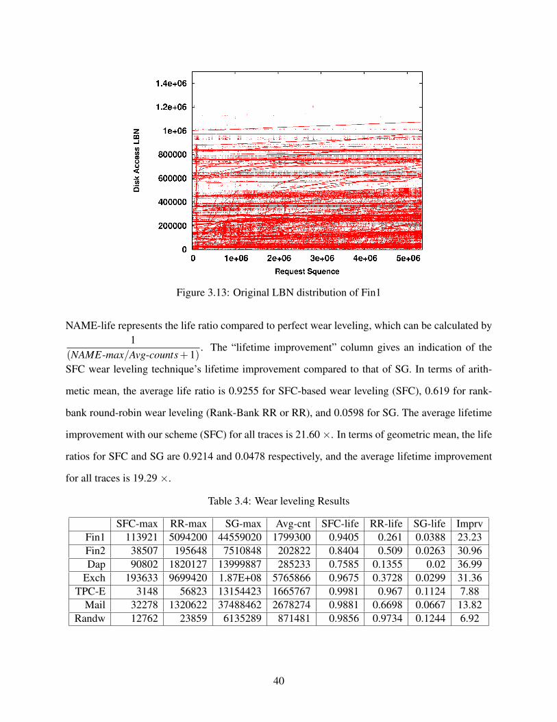
Figure 3.13: Original LBN distribution of Fin1
NAME-life represents the life ratio compared to perfect wear leveling, which can be calculated by1
(NAME-max/Avg-counts+1). The “lifetime improvement” column gives an indication of the
SFC wear leveling technique’s lifetime improvement compared to that of SG. In terms of arith-
metic mean, the average life ratio is 0.9255 for SFC-based wear leveling (SFC), 0.619 for rank-
bank round-robin wear leveling (Rank-Bank RR or RR), and 0.0598 for SG. The average lifetime
improvement with our scheme (SFC) for all traces is 21.60×. In terms of geometric mean, the life
ratios for SFC and SG are 0.9214 and 0.0478 respectively, and the average lifetime improvement
for all traces is 19.29 ×.
Table 3.4: Wear leveling Results
SFC-max RR-max SG-max Avg-cnt SFC-life RR-life SG-life ImprvFin1 113921 5094200 44559020 1799300 0.9405 0.261 0.0388 23.23Fin2 38507 195648 7510848 202822 0.8404 0.509 0.0263 30.96Dap 90802 1820127 13999887 285233 0.7585 0.1355 0.02 36.99
Exch 193633 9699420 1.87E+08 5765866 0.9675 0.3728 0.0299 31.36TPC-E 3148 56823 13154423 1665767 0.9981 0.967 0.1124 7.88
Mail 32278 1320622 37488462 2678274 0.9881 0.6698 0.0667 13.82Randw 12762 23859 6135289 871481 0.9856 0.9734 0.1244 6.92
40
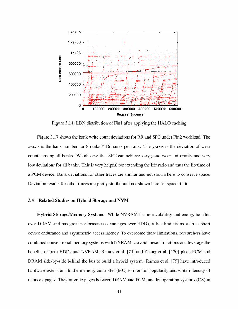
Figure 3.14: LBN distribution of Fin1 after applying the HALO caching
Figure 3.17 shows the bank write count deviations for RR and SFC under Fin2 workload. The
x-axis is the bank number for 8 ranks * 16 banks per rank. The y-axis is the deviation of wear
counts among all banks. We observe that SFC can achieve very good wear uniformity and very
low deviations for all banks. This is very helpful for extending the life ratio and thus the lifetime of
a PCM device. Bank deviations for other traces are similar and not shown here to conserve space.
Deviation results for other traces are pretty similar and not shown here for space limit.
3.4 Related Studies on Hybrid Storage and NVM
Hybrid Storage/Memory Systems: While NVRAM has non-volatility and energy benefits
over DRAM and has great performance advantages over HDDs, it has limitations such as short
device endurance and asymmetric access latency. To overcome these limitations, researchers have
combined conventional memory systems with NVRAM to avoid these limitations and leverage the
benefits of both HDDs and NVRAM. Ramos et al. [79] and Zhang et al. [120] place PCM and
DRAM side-by-side behind the bus to build a hybrid system. Ramos et al. [79] have introduced
hardware extensions to the memory controller (MC) to monitor popularity and write intensity of
memory pages. They migrate pages between DRAM and PCM, and let operating systems (OS) in
41
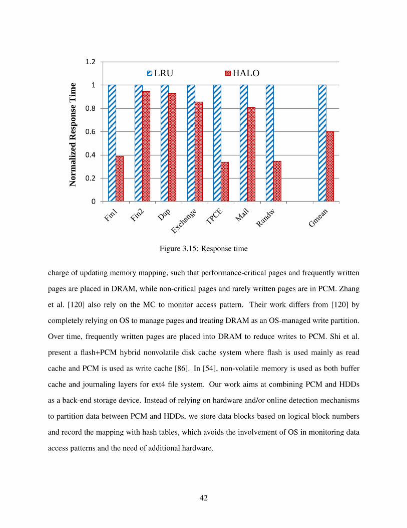
0
0.2
0.4
0.6
0.8
1
1.2
Norm
ali
zed
Res
pon
se T
ime
LRU HALO
Figure 3.15: Response time
charge of updating memory mapping, such that performance-critical pages and frequently written
pages are placed in DRAM, while non-critical pages and rarely written pages are in PCM. Zhang
et al. [120] also rely on the MC to monitor access pattern. Their work differs from [120] by
completely relying on OS to manage pages and treating DRAM as an OS-managed write partition.
Over time, frequently written pages are placed into DRAM to reduce writes to PCM. Shi et al.
present a flash+PCM hybrid nonvolatile disk cache system where flash is used mainly as read
cache and PCM is used as write cache [86]. In [54], non-volatile memory is used as both buffer
cache and journaling layers for ext4 file system. Our work aims at combining PCM and HDDs
as a back-end storage device. Instead of relying on hardware and/or online detection mechanisms
to partition data between PCM and HDDs, we store data blocks based on logical block numbers
and record the mapping with hash tables, which avoids the involvement of OS in monitoring data
access patterns and the need of additional hardware.
42
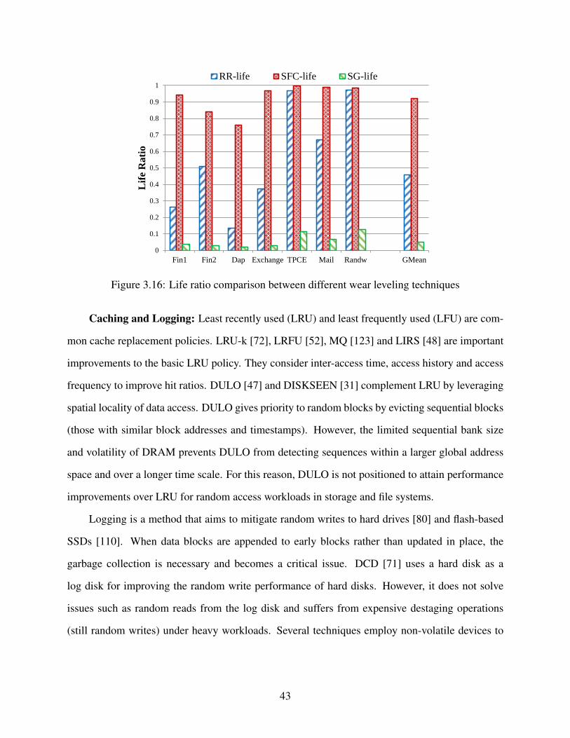
0
0.1
0.2
0.3
0.4
0.5
0.6
0.7
0.8
0.9
1
Fin1 Fin2 Dap Exchange TPCE Mail Randw GMean
Lif
e R
ati
o
RR-life SFC-life SG-life
Figure 3.16: Life ratio comparison between different wear leveling techniques
Caching and Logging: Least recently used (LRU) and least frequently used (LFU) are com-
mon cache replacement policies. LRU-k [72], LRFU [52], MQ [123] and LIRS [48] are important
improvements to the basic LRU policy. They consider inter-access time, access history and access
frequency to improve hit ratios. DULO [47] and DISKSEEN [31] complement LRU by leveraging
spatial locality of data access. DULO gives priority to random blocks by evicting sequential blocks
(those with similar block addresses and timestamps). However, the limited sequential bank size
and volatility of DRAM prevents DULO from detecting sequences within a larger global address
space and over a longer time scale. For this reason, DULO is not positioned to attain performance
improvements over LRU for random access workloads in storage and file systems.
Logging is a method that aims to mitigate random writes to hard drives [80] and flash-based
SSDs [110]. When data blocks are appended to early blocks rather than updated in place, the
garbage collection is necessary and becomes a critical issue. DCD [71] uses a hard disk as a
log disk for improving the random write performance of hard disks. However, it does not solve
issues such as random reads from the log disk and suffers from expensive destaging operations
(still random writes) under heavy workloads. Several techniques employ non-volatile devices to
43
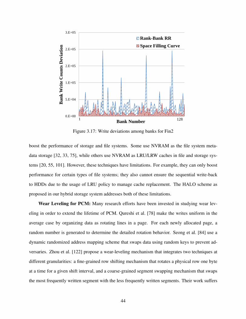
0.E+00
5.E+04
1.E+05
2.E+05
2.E+05
3.E+05
1 128
Ba
nk
Wri
te C
ou
nts
Dev
iati
on
Rank-Bank RR
Space Filling Curve
1 128 Bank Number
Figure 3.17: Write deviations among banks for Fin2
boost the performance of storage and file systems. Some use NVRAM as the file system meta-
data storage [32, 33, 75], while others use NVRAM as LRU/LRW caches in file and storage sys-
tems [20, 55, 101]. However, these techniques have limitations. For example, they can only boost
performance for certain types of file systems; they also cannot ensure the sequential write-back
to HDDs due to the usage of LRU policy to manage cache replacement. The HALO scheme as
proposed in our hybrid storage system addresses both of these limitations.
Wear Leveling for PCM: Many research efforts have been invested in studying wear lev-
eling in order to extend the lifetime of PCM. Qureshi et al. [78] make the writes uniform in the
average case by organizing data as rotating lines in a page. For each newly allocated page, a
random number is generated to determine the detailed rotation behavior. Seong et al. [84] use a
dynamic randomized address mapping scheme that swaps data using random keys to prevent ad-
versaries. Zhou et al. [122] propose a wear-leveling mechanism that integrates two techniques at
different granularities: a fine-grained row shifting mechanism that rotates a physical row one byte
at a time for a given shift interval, and a coarse-grained segment swapping mechanism that swaps
the most frequently written segment with the less frequently written segments. Their work suffers
44
from the overhead of hardware address mapping and the overhead of periodical sorting to pick
up appropriate segments for swapping. Ipek et al. [45] propose a solution to improve the lifetime
of PCM by replicating a single physical memory page over two faulty, otherwise unusable PCM
pages. With modifications to the memory controller, TLBs and OS, their work greatly improves
the lifetime of PCM. In [103], Wang et al. provide inter-set and intra-set wear-leveling techniques
to uniform write operations to ReRAM which is used as on-chip caches. Our wear leveling work
is distinguished from these prior efforts. We regard the global address space as a multidimen-
sional geometric space and employ a novel space filling curve-based algorithm to evenly distribute
accesses across different dimensions. Compared with existing work, our approach significantly
extends the lifetime of PCM in hybrid storage devices.
3.5 Summary
In this paper, we propose a new hybrid PCM+HDD storage system that leverages PCM as a
write cache to merge random write requests and improve access locality for the storage system.
Along with this, we also design a cache scheme, named HALO, which utilizes the fast access
and non-volatility features of PCM to improve system I/O performance with guaranteed reliabil-
ity. Results from a diverse set of workloads show that HALO can achieve lower traffic rates to
HDDs due to better caching and achieve higher system throughput led by smarter destaging tech-
niques. Therefore, our approaches reduce execution times significantly, 36.8% on average. This
hybrid storage organization is especially beneficial for workloads with intensive random writes.
We also design two wear leveling schemes, rank-bank round-robin wear leveling and space filling
curve based wear leveling, to extend the lifetime of PCM in the proposed hybrid devices. Our
results show that SFC-based wear leveling improves the life time of PCM devices by as much as
21.6 times. Also, we have integrated an in-house PCM simulator into DiskSim 4.0 [24] as a new
hardware model.
45
Chapter 4
I/O Optimization for a Large-Scale Climate Scientific Application
4.1 An Extensible Parallel I/O Framework
To overcome the limitations of existing design, especially to improve the performance at large
scale, a new framework that can support parallel I/O is imperative. One alternative approach to en-
able parallel I/O is to have all the participating processes write their own output independently.
However, such approach can generate a large number of small files, making it extremely difficult,
if not impossible, for post-processing software, such as visualization tool, to analyze the simulation
results. In addition, many parallel file systems, such as GPFS, provide poor performance on man-
aging small files due to high metadata overhead. Therefore, in this work, we take another approach
to designing a generalized framework that can leverage a rich set of state-of-the-art parallel I/O
techniques to eliminate the data gathering bottleneck in the original system, thereby accelerating
the output of simulation data. Figure 4.1 illustrates the new framework. Different from origi-
nal design in which root processes need to gather either plane data or bundle data before writing
the output into the file system, our new framework eliminates such limitation by enabling all the
participating processes to write their own data into a shared file in the parallel file system.
4.1.1 A Generalized and Portable Architecture
Different platforms have been optimized for different file formats. For example, many labo-
ratories have meticulously tuned PVFS [11] to efficiently support NetCDF format. Therefore, to
provide high portability across different platforms, we redesign the communication and I/O frame-
work of GEOS-5 as shown in Figure 4.1 to support three parallel I/O techniques, including parallel
NetCDF, NetCDF-4, and ADIOS. Despite the striking differences among these techniques, our
46
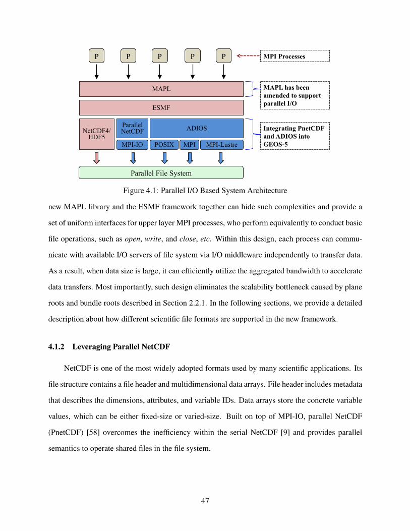
P P P P P
MAPL
Parallel NetCDF ADIOS NetCDF4/
HDF5
ESMF
MPI-IO POSIX MPI MPI-Lustre
Parallel File System
MPI Processes
MAPL has been amended to support parallel I/O
Integrating PnetCDF and ADIOS into GEOS-5
Figure 4.1: Parallel I/O Based System Architecture
new MAPL library and the ESMF framework together can hide such complexities and provide a
set of uniform interfaces for upper layer MPI processes, who perform equivalently to conduct basic
file operations, such as open, write, and close, etc. Within this design, each process can commu-
nicate with available I/O servers of file system via I/O middleware independently to transfer data.
As a result, when data size is large, it can efficiently utilize the aggregated bandwidth to accelerate
data transfers. Most importantly, such design eliminates the scalability bottleneck caused by plane
roots and bundle roots described in Section 2.2.1. In the following sections, we provide a detailed
description about how different scientific file formats are supported in the new framework.
4.1.2 Leveraging Parallel NetCDF
NetCDF is one of the most widely adopted formats used by many scientific applications. Its
file structure contains a file header and multidimensional data arrays. File header includes metadata
that describes the dimensions, attributes, and variable IDs. Data arrays store the concrete variable
values, which can be either fixed-size or varied-size. Built on top of MPI-IO, parallel NetCDF
(PnetCDF) [58] overcomes the inefficiency within the serial NetCDF [9] and provides parallel
semantics to operate shared files in the file system.
47
Our new framework strives to leverage the strength of PnetCDF. Each MPI process performs
computation on a chunk of plane data (as described in Section 2.2.1). At the end of each times-
tamp, instead of sending the data to the roots, each process directly writes the data into the shared
NetCDF file through specifying the offset to the starting point of the data array. The starting
point of the variable array is determined at the variable defining phase, which is conducted dur-
ing the file open phase. During the data writing, we adopt collective I/O methods provided by
PnetCDF in the current design. This means many I/O requests for non-contiguous portions of a
file are merged together by either I/O servers or working processes before being processed. Such
approach significantly reduces the number of I/O requests that need to be processed by the file
system, thus improving the performance. At the file open and close phases, NetCDF metadata,
such as dimension definition, variable attributes and lengths, needs to be synchronized among all
of the participating processes in the group. To achieve this, one process is elected as the leader of
the group to take charge of broadcasting the changes whenever metadata is modified. However,
our evaluation results show that maintaining strong metadata consistency can cause high overhead
when doing small bundle operations.
4.1.3 Integration of ADIOS
In order to leverage the asynchronous I/O of ADIOS to improve GEOS-5’s performance, we
integrate ADIOS into GEOS-5 as an ESMF component. ADIOS is able to provide the flexibil-
ity of switching back-end I/O methods at ease, such as the universal POSIX and MPI-IO meth-
ods. Meanwhile, ADIOS provides the easy-to-use plug-in mechanism to add new file system or
platform-specific I/O methods for optimal performance, such as MPI-Lustre.
Along with the integration of ADIOS, we use the BP file format [66] for processes to write
data to a shared file. BP is a self-describing and metadata rich file format that consists of a number
of process groups (each process group maintains data for one individual process) and a footer con-
taining the file’s metadata and index information. It can be easily transformed into other scientific
file formats, e.g., HDF5 and NetCDF.
48
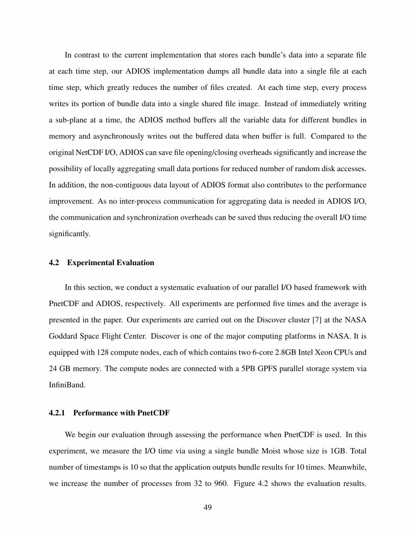
In contrast to the current implementation that stores each bundle’s data into a separate file
at each time step, our ADIOS implementation dumps all bundle data into a single file at each
time step, which greatly reduces the number of files created. At each time step, every process
writes its portion of bundle data into a single shared file image. Instead of immediately writing
a sub-plane at a time, the ADIOS method buffers all the variable data for different bundles in
memory and asynchronously writes out the buffered data when buffer is full. Compared to the
original NetCDF I/O, ADIOS can save file opening/closing overheads significantly and increase the
possibility of locally aggregating small data portions for reduced number of random disk accesses.
In addition, the non-contiguous data layout of ADIOS format also contributes to the performance
improvement. As no inter-process communication for aggregating data is needed in ADIOS I/O,
the communication and synchronization overheads can be saved thus reducing the overall I/O time
significantly.
4.2 Experimental Evaluation
In this section, we conduct a systematic evaluation of our parallel I/O based framework with
PnetCDF and ADIOS, respectively. All experiments are performed five times and the average is
presented in the paper. Our experiments are carried out on the Discover cluster [7] at the NASA
Goddard Space Flight Center. Discover is one of the major computing platforms in NASA. It is
equipped with 128 compute nodes, each of which contains two 6-core 2.8GB Intel Xeon CPUs and
24 GB memory. The compute nodes are connected with a 5PB GPFS parallel storage system via
InfiniBand.
4.2.1 Performance with PnetCDF
We begin our evaluation through assessing the performance when PnetCDF is used. In this
experiment, we measure the I/O time via using a single bundle Moist whose size is 1GB. Total
number of timestamps is 10 so that the application outputs bundle results for 10 times. Meanwhile,
we increase the number of processes from 32 to 960. Figure 4.2 shows the evaluation results.
49
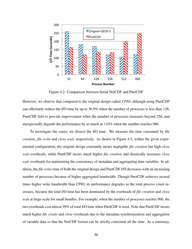
0
50
100
150
200
250
300
32 64 128 256 512 960
I/O Tim
e (secon
ds)
Process Number
Original GEOS-‐5
PnetCDF
Figure 4.2: Comparison between Serial NetCDF and PnetCDF
However, we observe that compared to the original design called CFIO, although using PnetCDF
can efficiently reduce the I/O time by up to 36.9% when the number of processes is less than 128,
PnetCDF fails to provide improvement when the number of processes increases beyond 256, and
unexpectedly degrade the performance by as much as 110% when the number reaches 960.
To investigate the cause, we dissect the I/O time. We measure the time consumed by file
creation, file write and close wait, respectively. As shown in Figure 4.3, within the given exper-
imental configuration, the original design constantly incurs negligible file creation but high close
wait overheads, while PnetCDF incurs much higher file creation and drastically increases close
wait overheads for maintaining the consistency of metadata and aggregating data variables. In ad-
dition, the file write time of both the original design and PnetCDF I/O decreases with an increasing
number of processes because of higher aggregated bandwidth. Though PnetCDF achieves several
times higher write bandwidth than CFIO, its performance degrades as the total process count in-
creases, because the total I/O time has been dominated by the overheads of file creation and close
wait at large-scale for small bundles. For example, when the number of processes reaches 960, the
two overheads cost almost 99% of total I/O time when PnetCDF is used. Note that PnetCDF incurs
much higher file create and close overheads due to the metadata synchronization and aggregation
of variable data so that the NetCDF format can be strictly consistent all the time. As a summary,
50
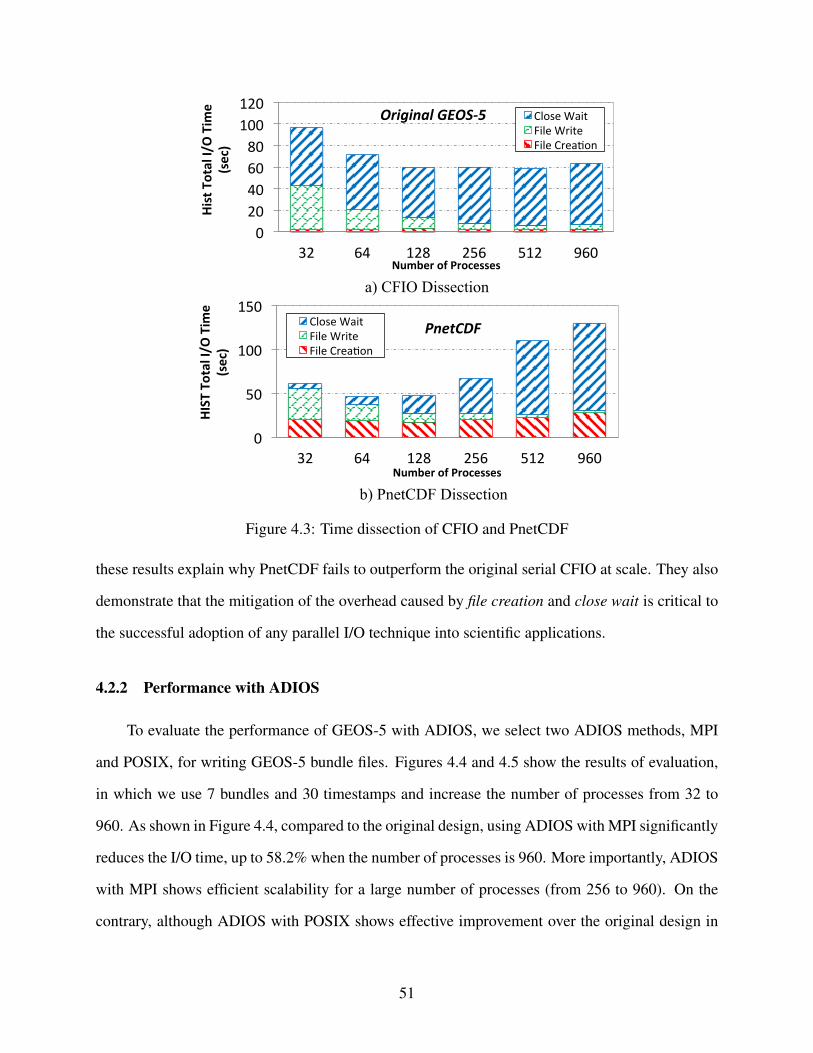
0
50
100
150
32 64 128 256 512 960
HIST Total I/O Tim
e (sec)
Number of Processes
Close Wait File Write File Crea6on
PnetCDF
0 20 40 60 80
100 120
32 64 128 256 512 960
Hist Total I/O Tim
e (sec)
Number of Processes
Close Wait File Write File Crea6on
Original GEOS-‐5
a) CFIO Dissection
b) PnetCDF Dissection
Figure 4.3: Time dissection of CFIO and PnetCDF
these results explain why PnetCDF fails to outperform the original serial CFIO at scale. They also
demonstrate that the mitigation of the overhead caused by file creation and close wait is critical to
the successful adoption of any parallel I/O technique into scientific applications.
4.2.2 Performance with ADIOS
To evaluate the performance of GEOS-5 with ADIOS, we select two ADIOS methods, MPI
and POSIX, for writing GEOS-5 bundle files. Figures 4.4 and 4.5 show the results of evaluation,
in which we use 7 bundles and 30 timestamps and increase the number of processes from 32 to
960. As shown in Figure 4.4, compared to the original design, using ADIOS with MPI significantly
reduces the I/O time, up to 58.2% when the number of processes is 960. More importantly, ADIOS
with MPI shows efficient scalability for a large number of processes (from 256 to 960). On the
contrary, although ADIOS with POSIX shows effective improvement over the original design in
51
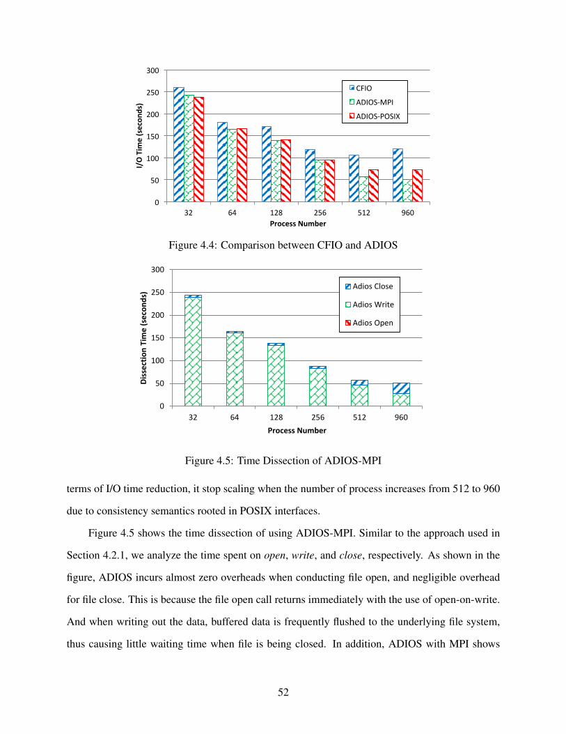
0
50
100
150
200
250
300
32 64 128 256 512 960
I/O Tim
e (secon
ds)
Process Number
CFIO
ADIOS-‐MPI
ADIOS-‐POSIX
Figure 4.4: Comparison between CFIO and ADIOS
0
50
100
150
200
250
300
32 64 128 256 512 960
Dis
sect
ion
Tim
e (
seco
nd
s)
Process Number
Adios Close
Adios Write
Adios Open
Figure 4.5: Time Dissection of ADIOS-MPI
terms of I/O time reduction, it stop scaling when the number of process increases from 512 to 960
due to consistency semantics rooted in POSIX interfaces.
Figure 4.5 shows the time dissection of using ADIOS-MPI. Similar to the approach used in
Section 4.2.1, we analyze the time spent on open, write, and close, respectively. As shown in the
figure, ADIOS incurs almost zero overheads when conducting file open, and negligible overhead
for file close. This is because the file open call returns immediately with the use of open-on-write.
And when writing out the data, buffered data is frequently flushed to the underlying file system,
thus causing little waiting time when file is being closed. In addition, ADIOS with MPI shows
52
scalable file writing with an increasing number of processes, decreasing from 90% of I/O time
to 56% of I/O time. This is because of the higher aggregated bandwidth achieved with a large
number of processes. Compared with PnetCDF, using ADIOS efficiently mitigates the overhead
of maintaining the metadata of shared file, thus achieving better scalability and performance at
large-scale.
4.3 Related Studies on I/O optimizations for scientific applications
There is a large body of research literature on improving the I/O performance of scientific
applications on large-scale supercomputing systems. Many I/O techniques have been designed
to exploit the best I/O performance from underlying file systems. These include NetCDF-4 [98],
HDF-5 [93, 67], PnetCDF [58] and ADIOS [1]. Built on top of these techniques, more efforts have
been taken to study optimizations such as data buffering [61], file striping [116], subfiling [22, 27],
staging [16] and data reorganization for multidimensional data structure [82, 87, 95, 96, 97]. Some
of the techniques have been adopted into various I/O middleware libraries.
There is also a rich set of literatures on the performance characterization of HPC systems,
spanning a wide variety of aspects such as inter-process communication [112], interconnect tech-
nologies, parallel file systems, reading patterns [65] and power management. Many studies are
closely related to ours. [35, 44, 114, 115] reported scaling trends of the performance for various
I/O patterns on Cray XT platforms. [53] described the challenges to improve the I/O performance
and scalability on IBM Blue Gene/P systems. [81] characterized the I/O performance of NASA
applications on Pleiades. Our work is different from the aforementioned studies. We focus on
a climate application GEOS-5 that has a communication and I/O pattern representative of vari-
ous climate and earth modeling applications. For this pattern, we introduce an extensible parallel
framework that can employ different parallel I/O techniques such as PnetCDF and ADIOS and
optimize the I/O performance of climate application.
53

4.4 Summary
In this work, we target at identifying and addressing influential factors that can hinder current
scientific applications from achieving efficient I/O. By adopting the GEOS-5 climate modeling
application as our case study, we analyze the typical communication and I/O patterns in repre-
sentative scientific applications. And we discover that many legacy scientific applications employ
similar hierarchical network aggregation to collect data portions for multi-dimensional variables
from all processes and then dump the aggregated data into persistent storage. Through compre-
hensive measurements on the NASA discover cluster, we quantitatively profile and dissect the
network communication and I/O costs by such I/O schemes. In order to address the drawbacks
of single point of network contention and under-parallelized I/O patterns, we modify the current
I/O framework of GEOS-5, enabling the applications to take advantage of state-of-art parallel I/O
techniques like PnetCDF and ADIOS. Experimental results demonstrate that the integrated parallel
I/O techniques supported by our I/O framework can improve the application I/O time at various
scales. This performance improvement come from the elimination of huge amounts of network
aggregation and significantly promoted I/O concurrency.
In the future, we plan to study asynchronous I/O schemes and efficient burst buffering tech-
niques for further I/O performance improvements of scientific applications.
54
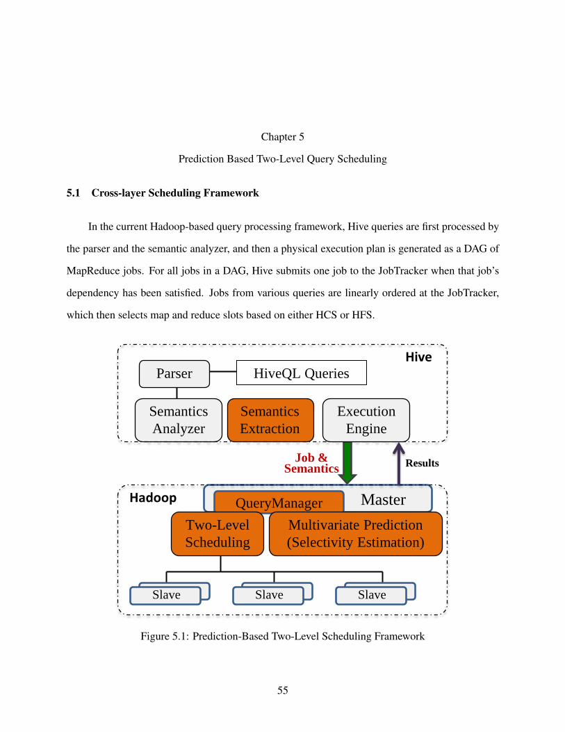
Chapter 5
Prediction Based Two-Level Query Scheduling
5.1 Cross-layer Scheduling Framework
In the current Hadoop-based query processing framework, Hive queries are first processed by
the parser and the semantic analyzer, and then a physical execution plan is generated as a DAG of
MapReduce jobs. For all jobs in a DAG, Hive submits one job to the JobTracker when that job’s
dependency has been satisfied. Jobs from various queries are linearly ordered at the JobTracker,
which then selects map and reduce slots based on either HCS or HFS.
Master
Slave
Hadoop QueryManager
Semantics
Extraction
Slave Slave
Two-Level
Scheduling
Multivariate Prediction
(Selectivity Estimation)
Execution
Engine
Parser
Semantics
Analyzer
HiveQL Queries
Job & Semantics
Results
Hive
Figure 5.1: Prediction-Based Two-Level Scheduling Framework
55
Clearly, all the query-level semantics is lost when Hadoop receives a job from Hive. In addi-
tion, the Hadoop JobTracker can only see the presence of individual jobs, not their parent queries.
As a result, there is no coordination among jobs to ensure the best overall progress for the query,
not just that of the individual jobs.
To address the aforementioned challenges systematically, we propose a cross-layer two-level
scheduling framework. As shown in Figure 5.1, three techniques are introduced including seman-
tics extraction and percolation, multivariate execution-time prediction with selectivity estimation,
and two-level query scheduling.
Semantics Extraction and Percolation: First, we introduce a component for semantics ex-
traction and percolation in Hive during the query compilation and its execution plan construction.
To bridge the semantic gap between Hive and Hadoop, we extract the semantics from each query’s
logical and physical plans. This includes these query attributes: the DAG of jobs, the dependencies
among jobs, the operators and predicates of jobs, and the input tables. When Hive submits a job
to Hadoop, it includes its semantics information as part of the job configuration file. Instead of
directly queuing a job, our framework maintains a queue of all queries, and adds each job along
with related semantics to its parent query.
Second, across both Hive and Hadoop layers, we introduce a scheme for multivariate execution-
time prediction. This scheme includes a selectivity estimator that can evaluate query predicates and
estimate the changing size of data during the query execution, and a regression model that predicts
the job execution time. The percolated semantics is leveraged by both the selectivity estimator and
the regression model.
Finally, at the Hadoop layer we introduce two-level query scheduling to (1) manage the ad-
mission and concurrency of queries to ensure efficient resource utilization and fair progress among
different queries at a coarse-grained inter-query level; and (2) leverage percolated semantics and
estimate the progress of jobs at the intra-query level, and accordingly prioritize jobs on the critical
path of a query DAG for execution.
56
Multivariate time prediction and two-level query scheduling are described in detail in Sec-
tions 5.2 and 5.3, respectively.
5.2 Query prediction model
To achieve the objective of efficient two-level query scheduling, accurate prediction of the
execution time and resource usage for a query is a crucial prerequisite. We apply a job-oriented
time estimation rather than a query-oriented time estimation approach [38] in MapReduce because
of two reasons. First, in MapReduce-based data warehouses, a query is divided into multiple
MapReduce jobs, each with a separate scan of its input tables, materialization and de/serialization;
second, intra-query job parallelism can affect query execution time. Therefore, job-oriented time
estimation/modeling can gain insights about execution statistics and dynamic behaviors of jobs
inside a query, therefore presents a better fit.
In order to have an accurate prediction of job execution time, we need to decide what seman-
tics to include as parameters in the model. In addition, there are multiple steps of data movement
during the execution of a job, and the data size changes inside a job and along the DAG of a query.
Thus a good prediction model also needs to reflect such dynamics of data [34]. To this end, we
first describe the selectivity estimation of MapReduce jobs and then elaborate the integration of
selectivity estimation into the prediction.
5.2.1 Selectivity Estimation
As shown in Figure 5.2, for a MapReduce job in a query DAG, the output of its map tasks
provides the input for its reduce tasks. One job’s output is often taken as part of the input of
its succeeding job in the same DAG. The input size of a job directly affects its resource usage
(number of map and reduce tasks) during execution in MapReduce. In addition, the data size of
map output (intermediate data) also significantly affects the execution time of reduce tasks, and
indirectly affects the execution of the downstream jobs in the query. An accurate prediction of
57
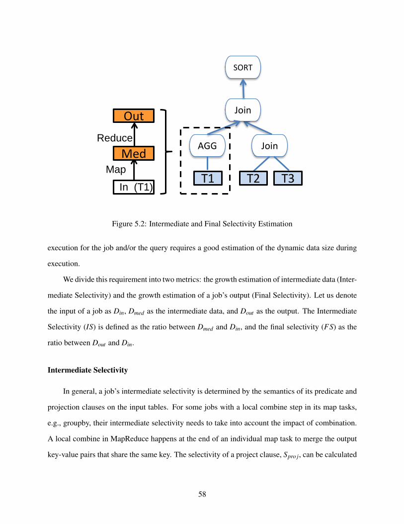
AGG
Join
Join
SORT
T1 T2 T3
Med
Out
Map
Reduce
In (T1)
Figure 5.2: Intermediate and Final Selectivity Estimation
execution for the job and/or the query requires a good estimation of the dynamic data size during
execution.
We divide this requirement into two metrics: the growth estimation of intermediate data (Inter-
mediate Selectivity) and the growth estimation of a job’s output (Final Selectivity). Let us denote
the input of a job as Din, Dmed as the intermediate data, and Dout as the output. The Intermediate
Selectivity (IS) is defined as the ratio between Dmed and Din, and the final selectivity (FS) as the
ratio between Dout and Din.
Intermediate Selectivity
In general, a job’s intermediate selectivity is determined by the semantics of its predicate and
projection clauses on the input tables. For some jobs with a local combine step in its map tasks,
e.g., groupby, their intermediate selectivity needs to take into account the impact of combination.
A local combine in MapReduce happens at the end of an individual map task to merge the output
key-value pairs that share the same key. The selectivity of a project clause, Spro j, can be calculated
58
as the ratio between the average width of the selected attributes and the average tuple size in a
table. We rely on the table statistics information for estimating Spro j.
Let us denote |In| and |Med| as the numbers of tuples in the input table and the inter-
mediate data, respectively. The selectivity of a predicate clause, Spred , can be calculated as
Spred = |Med|/|In| if there is no local combine operation in the map tasks. We build off-line
histograms for the attributes of the input table for estimating Spred . Assuming piece-wise uniform
distribution of attribute values, equi-width histograms [76] are built on tables’ attributes to be fil-
tered through a MapReduce job and stored on HDFS. An equi-width histogram is built by first
splitting the domain of an attribute uniformly into a given number of buckets and then recording
the number of values and distinct values in each bucket [76]. For scale values, such as integer,
double and date, we compute the selectivity of predicate clauses by counting the number of tu-
ples in the matching buckets. For text values, such as string, we avoid complex and expensive
structures such as suffix trees, and only record the numbers of distinct and total values, as well as
history selectivities if possible, for a best-effort selectivity estimation. For a conjunctive predicate
formed by multiple predicate clauses that filter multiple tables on different attributes, we assume
the distribution independence of attributes and compute the overall selectivity Spred as the product
of selectivities from all predicate clauses.
Hive and Pig queries are compiled into DAGs of operators. In these DAGs, the operators
for global shuffle/aggregation will be converted into separated MapReduce jobs. We term such
operators as major operators, e.g., groupby, orderby and join. Other operators will be carried
out with the map phase of a job. We term such operators as minor operators, e.g., normal range
and equality predicates. We categorize jobs into three types with respect to their major operators:
groupby, join and extract (including orderby and all other major operators).
We elaborate further on our estimation of IS. Our discuss focuses on the aforementioned three
operations: extract, groupby and join. Other operations can be considered as simple or composite
derivatives of these three.
59
Extract: An extract operation usually scans one input table, we calculate its intermediate
selectivity as IS = Spred ∗Spro j.
Groupby: In a groupby operation, its local combine can further reduce the intermediate
data. Let Scomb denote the combination selectivity. We can calculate its intermediate selectivity
as IS = Scomb ∗ Spro j. The calculation of Scomb needs to be elaborated further with an example.
Suppose a job performs a groupby operation on Table T’s key x and key y. Let T.dxy denote the
product from the numbers of distinct keys for x and y. If the groupby keys are all clustered in the
table, Scomb is calculated as Scomb = min(1, T.dxy|T |∗Spred
) ∗ Spred = min(Spred,T.dxy|T | ). Otherwise, if the
groupby keys are randomly distributed, Scomb is then calculated as Scomb = min(Spred,T.dxy
|T |/Nmaps),
where Nmaps denotes the number of map tasks of the job. We omit the calculation for other minor
cases.
Join: A join operation may select tuples from two or more input tables. We describe the
calculation of IS for a simple join job of two tables. Let r1 represent the percentage of one table’s
data in the total input of a job, r2 = (1− r1) for the other table. We can calculate IS for a join job
with two input tables as: IS = Spred 1 ∗Spro j 1 ∗ r1 +Spred 2 ∗Spro j 2 ∗ (1− r1).
Final Selectivity
Let us denote |Out| as the number of tuples and Wout the average width of tuples in the output
(Out), a job’s final selectivity is calculated as FS = |Out| ∗WOut/DIn. The key of calculating FS is
to compute |Out|. Our discussion focuses on three common operations including extract, groupby
and join.
Extract: In Hive, there are two common extract operations, “limit k” and “order by”. For the
former, |Out|= min(|In|,k); and for the latter, |Out|= |In|.
Groupby: A groupby operation may use one or more keys. The number tuples in the output is
determined by the cardinalities of the keys and the predicates on the keys. We show the calculation
for an example operation with one key. For a table T , let us denote the cardinality of a key x as
T.dx. A groupby operation on key x will have |Out|= min(T.dx, |T | ∗Spred).
60
Join: There are many variations of join operations. Multiple operations may hierarchically
formulate as a join tree. We focus on a few common join operations with two or three tables
to illustrate the calculation and the most important case: equi-join between a primary key and a
foreign key (and tables should obey referential integrity).
An equi-join operation from these two tables T1 and T2 will have |Out| = |T1 ./ T2| = |T1| ∗
|T2| ∗ 1max(T1.dx, T2.dx)
if join keys follow uniform distribution [91]. However, uniform distribution
is rare in practical cases; in addition, this approach only applies for multiple joins that share a
common join key. In our work, we assume piece-wise uniform distribution, where in each equi-
width bucket keys follow uniform distribution. Let T1i denote the i-th bucket of in the equi-width
histogram for a join operation on Key x. Then we can calculate the number of tuples in a join job’s
result set as:
|T1 ./ T2|=n
∑i=1|T1i| ∗ |T2i| ∗
1max(T1i.dx, T2i.dx)
(5.1)
Since (T1i ./ T2i).dx = min(T1i.dx, T2i.dx), the equation above can be evolved to calculate the
join selectivity for shared-key joins on three or more tables.
For chained joins with unshared keys, e.g., T1 and T2 joining on Key x and T2 and T3 joining
on Key y, we leverage the techniques introduced in [21] by acquiring the updated piece-wise dis-
tribution of Key y after the first join for selectivity estimation of cascaded joins. For natural joins
(each operator joins one table’s primary key with another table’s foreign key) with local predicates
on each table, selectivities are accumulated along branches of the join tree, thus the number of
tuples in the result set can be approximated as:
|T1.pred1 ./ T2.pred2 ./ · · · ./ Tn.predn|
= Spred 1Spred 2 . . .Spred n max(|T1|, |T2|, . . . , |Tn|)(5.2)
An Example of Selectivity Estimation
We use a modified TPC-H [13] query Q11 as an example to demonstrate the estimation of
selectivities. Figure 5.3 shows the flow of selectivity estimation. This query is transformed into
61
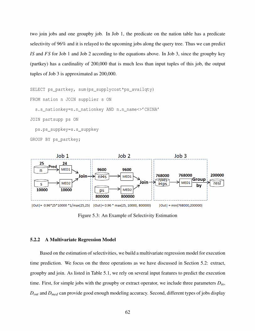
two join jobs and one groupby job. In Job 1, the predicate on the nation table has a predicate
selectivity of 96% and it is relayed to the upcoming jobs along the query tree. Thus we can predict
IS and FS for Job 1 and Job 2 according to the equations above. In Job 3, since the groupby key
(partkey) has a cardinality of 200,000 that is much less than input tuples of this job, the output
tuples of Job 3 is approximated as 200,000.
SELECT ps_partkey, sum(ps_supplycost*ps_availqty)
FROM nation n JOIN supplier s ON
s.s_nationkey=n.n_nationkey AND n.n_name<>’CHINA’
JOIN partsupp ps ON
ps.ps_suppkey=s.s_suppkey
GROUP BY ps_partkey;
Figure 5.3: An Example of Selectivity Estimation
5.2.2 A Multivariate Regression Model
Based on the estimation of selectivities, we build a multivariate regression model for execution
time prediction. We focus on the three operations as we have discussed in Section 5.2: extract,
groupby and join. As listed in Table 5.1, we rely on several input features to predict the execution
time. First, for simple jobs with the groupby or extract operator, we include three parameters Din,
Dout and Dmed can provide good enough modeling accuracy. Second, different types of jobs display
62
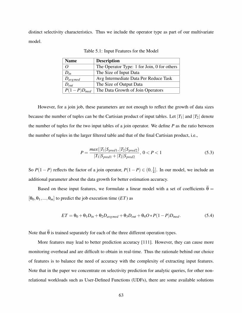
distinct selectivity characteristics. Thus we include the operator type as part of our multivariate
model.
Table 5.1: Input Features for the Model
Name DescriptionO The Operator Type: 1 for Join, 0 for othersDin The Size of Input DataDavgmed Avg Intermediate Data Per Reduce TaskDout The Size of Output DataP(1−P)Dmed The Data Growth of Join Operators
However, for a join job, these parameters are not enough to reflect the growth of data sizes
because the number of tuples can be the Cartisian product of input tables. Let |T1| and |T2| denote
the number of tuples for the two input tables of a join operator. We define P as the ratio between
the number of tuples in the larger filtered table and that of the final Cartisian product, i.e.,
P =max(|T1|Spred1, |T2|Spred2)
|T1|Spred1 + |T2|Spred2, 0 < P < 1 (5.3)
So P(1−P) reflects the factor of a join operator, P(1−P) ∈ (0, 14 ]. In our model, we include an
additional parameter about the data growth for better estimation accuracy.
Based on these input features, we formulate a linear model with a set of coefficients ~θ =
[θ0,θ1, ...,θm] to predict the job execution time (ET ) as
ET = θ0 +θ1Din +θ2Davgmed +θ3Dout +θ4O∗P(1−P)Dmed. (5.4)
Note that~θ is trained separately for each of the three different operation types.
More features may lead to better prediction accuracy [111]. However, they can cause more
monitoring overhead and are difficult to obtain in real-time. Thus the rationale behind our choice
of features is to balance the need of accuracy with the complexity of extracting input features.
Note that in the paper we concentrate on selectivity prediction for analytic queries, for other non-
relational workloads such as User-Defined Functions (UDFs), there are some available solutions
63
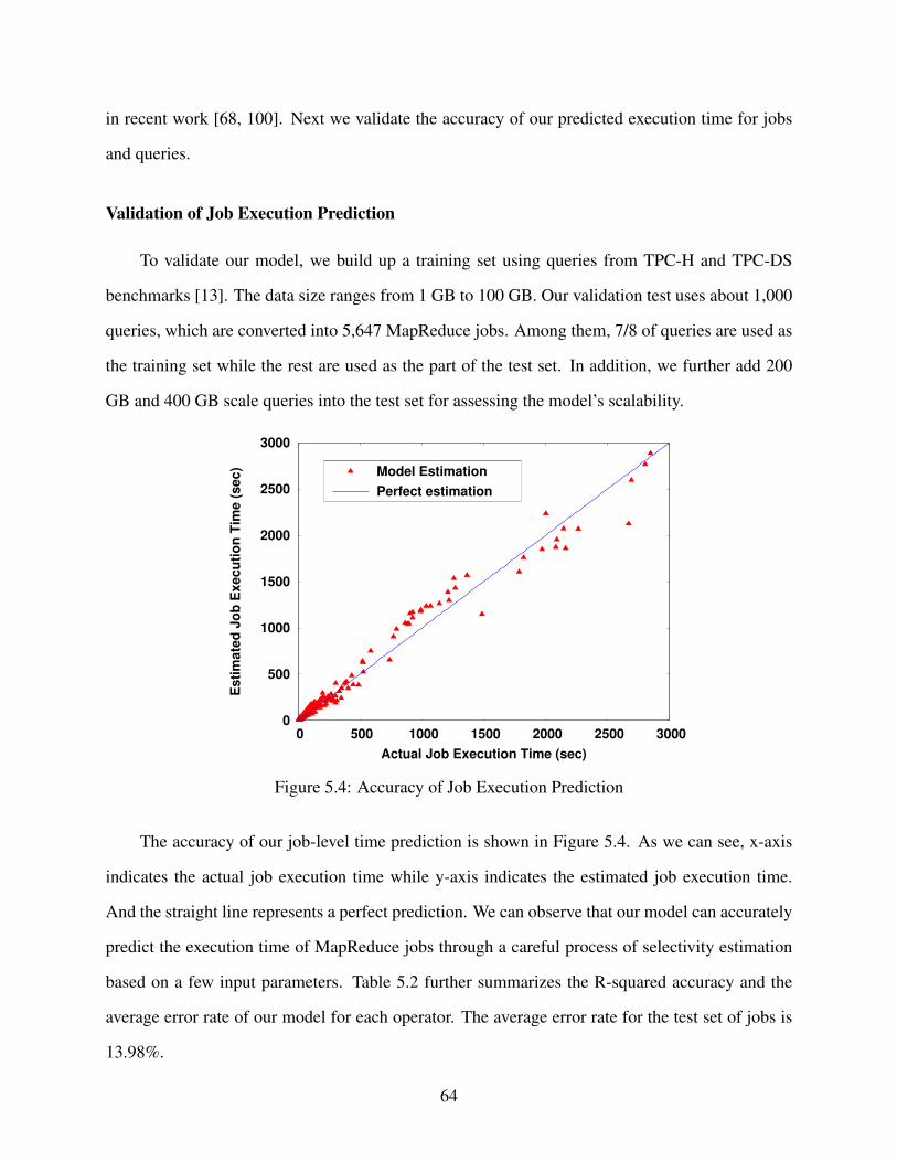
in recent work [68, 100]. Next we validate the accuracy of our predicted execution time for jobs
and queries.
Validation of Job Execution Prediction
To validate our model, we build up a training set using queries from TPC-H and TPC-DS
benchmarks [13]. The data size ranges from 1 GB to 100 GB. Our validation test uses about 1,000
queries, which are converted into 5,647 MapReduce jobs. Among them, 7/8 of queries are used as
the training set while the rest are used as the part of the test set. In addition, we further add 200
GB and 400 GB scale queries into the test set for assessing the model’s scalability.
0
500
1000
1500
2000
2500
3000
0 500 1000 1500 2000 2500 3000
Esti
mate
d J
ob
Execu
tio
n T
ime (
sec)
Actual Job Execution Time (sec)
Model Estimation
Perfect estimation
Figure 5.4: Accuracy of Job Execution Prediction
The accuracy of our job-level time prediction is shown in Figure 5.4. As we can see, x-axis
indicates the actual job execution time while y-axis indicates the estimated job execution time.
And the straight line represents a perfect prediction. We can observe that our model can accurately
predict the execution time of MapReduce jobs through a careful process of selectivity estimation
based on a few input parameters. Table 5.2 further summarizes the R-squared accuracy and the
average error rate of our model for each operator. The average error rate for the test set of jobs is
13.98%.
64
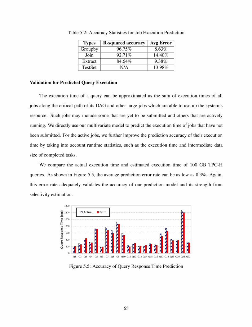
Table 5.2: Accuracy Statistics for Job Execution Prediction
Types R-squared accuracy Avg ErrorGroupby 96.75% 8.63%
Join 92.71% 14.40%Extract 84.64% 9.38%TestSet N/A 13.98%
Validation for Predicted Query Execution
The execution time of a query can be approximated as the sum of execution times of all
jobs along the critical path of its DAG and other large jobs which are able to use up the system’s
resource. Such jobs may include some that are yet to be submitted and others that are actively
running. We directly use our multivariate model to predict the execution time of jobs that have not
been submitted. For the active jobs, we further improve the prediction accuracy of their execution
time by taking into account runtime statistics, such as the execution time and intermediate data
size of completed tasks.
We compare the actual execution time and estimated execution time of 100 GB TPC-H
queries. As shown in Figure 5.5, the average prediction error rate can be as low as 8.3%. Again,
this error rate adequately validates the accuracy of our prediction model and its strength from
selectivity estimation.
0
200
400
600
800
1000
1200
1400
Q1 Q2 Q3 Q4 Q5 Q6 Q7 Q8 Q9 Q10 Q11 Q12 Q13 Q14 Q15 Q16 Q17 Q18 Q19 Q20 Q21 Q22
Qu
ery
Re
spo
nse
Tim
e (
sec)
Actual Estm
Figure 5.5: Accuracy of Query Response Time Prediction
65
5.3 Two-level Query Scheduling
Based on the multivariate query model, our objective is to schedule the queries for better
resource utilization, efficiency and fairness. We propose to schedule queries and their internal
tasks and jobs at two levels. At the coarse-grained query level, an inter-query scheduler selects
queries for system efficiency and ensures fairness among concurrent queries. At the fine-grained
job level, an intra-query scheduler leverages the DAG semantics in a query and prioritizes critical-
path jobs based on our multivariate model.
5.3.1 Inter-Query Scheduling
When analytic queries are first submitted to our scheduling framework, we admit the query
and initialize the structure to keep track of its runtime information according to our multivariate
model. A query queue (Lact) is maintained for the active queries each of which contains a DAG of
runnable or running jobs. We apply our selectivity estimation and multivariate model recursively
from the largest depth of the query DAG to the smallest depth, i.e. the root node. To be specific,
DIn, IS, DMed , FS and DOut are initialized based on the job type, predicate and projection selec-
tivities as mentioned in Section 5.2. When one task has completed, we will update the number of
remaining tasks for this query. When one job is completed, we recursively update our estimation
of input, output and execution time for the downstream jobs along the DAG.
Selection Metric – Weighted Resource Demand
We need to ensure all queries be fairly treated with comparable slowdown ratios so that small
queries can turn around faster while big queries still get their fair share of time and resources for
execution if delayed by a certain degree. However, in selecting queries that are organized as DAGs
of jobs, we cannot solely rely on the temporal resource demand of a query, i.e. its remaining time
that can be estimated from our multivariate model. A query and all of its jobs often employ a
dynamic number of tasks during its execution. Each task may have its own execution time, CPU,
memory and I/O resource demand. Therefore, we introduce a simple metric to take into account
66
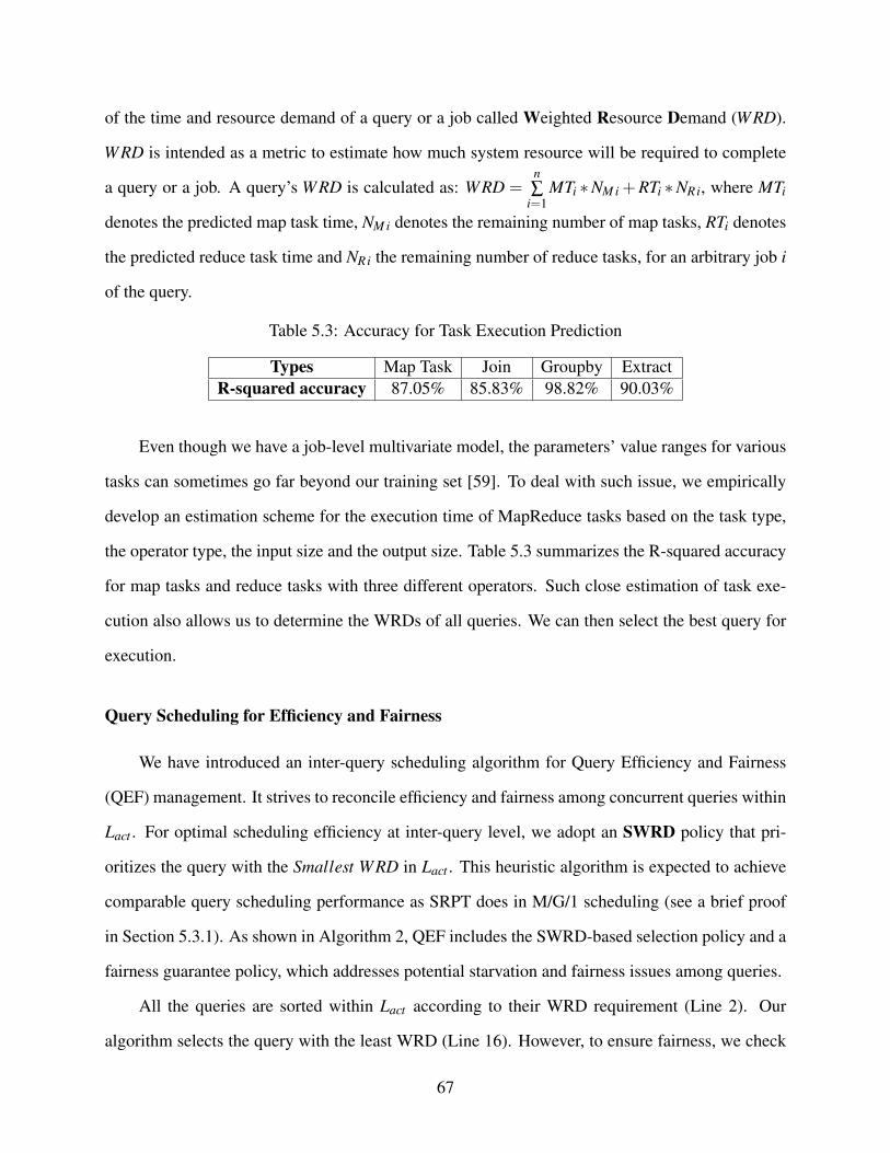
of the time and resource demand of a query or a job called Weighted Resource Demand (WRD).
WRD is intended as a metric to estimate how much system resource will be required to complete
a query or a job. A query’s WRD is calculated as: WRD =n∑
i=1MTi ∗NM i +RTi ∗NRi, where MTi
denotes the predicted map task time, NM i denotes the remaining number of map tasks, RTi denotes
the predicted reduce task time and NRi the remaining number of reduce tasks, for an arbitrary job i
of the query.
Table 5.3: Accuracy for Task Execution Prediction
Types Map Task Join Groupby ExtractR-squared accuracy 87.05% 85.83% 98.82% 90.03%
Even though we have a job-level multivariate model, the parameters’ value ranges for various
tasks can sometimes go far beyond our training set [59]. To deal with such issue, we empirically
develop an estimation scheme for the execution time of MapReduce tasks based on the task type,
the operator type, the input size and the output size. Table 5.3 summarizes the R-squared accuracy
for map tasks and reduce tasks with three different operators. Such close estimation of task exe-
cution also allows us to determine the WRDs of all queries. We can then select the best query for
execution.
Query Scheduling for Efficiency and Fairness
We have introduced an inter-query scheduling algorithm for Query Efficiency and Fairness
(QEF) management. It strives to reconcile efficiency and fairness among concurrent queries within
Lact . For optimal scheduling efficiency at inter-query level, we adopt an SWRD policy that pri-
oritizes the query with the Smallest WRD in Lact . This heuristic algorithm is expected to achieve
comparable query scheduling performance as SRPT does in M/G/1 scheduling (see a brief proof
in Section 5.3.1). As shown in Algorithm 2, QEF includes the SWRD-based selection policy and a
fairness guarantee policy, which addresses potential starvation and fairness issues among queries.
All the queries are sorted within Lact according to their WRD requirement (Line 2). Our
algorithm selects the query with the least WRD (Line 16). However, to ensure fairness, we check
67
Lact for a query that has been severely slowed down and prioritize it (Lines 5-8). Meanwhile, a
query with slow progress is also put into another list Lslow (Lines 9-11). QEF checks the size of
Lslow to decide in which list of queries to select the next query.
To measure the slowdown experienced by each query, we consider query’s sojourn time
Tso journ and estimated remaining execution time Trem. Specifically, the slowdown is defined as
slowdown =Tso journ+Trem
Talone. Talone denotes the estimated execution time when it runs alone in the
system. Trem and Talone are predicted based on our multivariate model. Meanwhile, the threshold
Dthreshold that determines whether a query has been unfairly treated is computed as 11−ρ
, where
ρ is the accumulated load on the system. Such threshold exhibits expected slowdown with the
Processor-Sharing (PS) policy as proven by M/G/1 model [109].
Algorithm 2 Query Efficiency and Fairness Management
1: Lact : {a list of queries in the ascending order of WRD.}2: Lslow:{a list of queries that have exceeded the slowdown threshold in the ascending order.}3: for all Q ∈ Lact do4: if (Q.slowdown > 2×Dthreshold) then5: Schedule Q via Algorithm 36: Return7: end if8: if (Q.slowdown > Dthreshold) then9: Lslow.add(Q)
10: end if11: end for12: if sizeo f (Lslow)> Limitslow then13: Qsched ← {last query in Lslow}14: else15: Qsched ← {first query in Lact} //SWRD16: end if17: Schedule Qsched via Algorithm 3
Proof for SWRD
According to Little’s Law [51], a schedule for minimizing average response time translates to
a schedule for minimizing the average query number in a system. Let N(t)SWRD and N(t)ϕ denote
the number of queries residing in the system for SWRD scheduling policy and any other policy. For
68
the J queries with largest WRD and J <= min(N(t)SWRD, N(t)ϕ), we have ∑Ji=1WRDSWRD
i <=
∑Ji=1WRDϕ
i because SWRD favors the queries with smallest WRD. With the assumption of not
considering the possible resource utilization difference caused by job phase independence and
intra-query job dependence, the remaining workloads (WRD) at any time should be the same
for any scheduling algorithm, thus we have ∑N(t)SWRD
i=1 WRDSWRDi = ∑
N(t)ϕ
i=1 WRDϕ
i . Therefore,
N(t)SWRD <= N(t)ϕ.
5.3.2 Intra-Query Scheduling
At the intra-query level, our target is to minimize the makespan of a query that consists of a
DAG of MapReduce jobs. This problem is analogous to the multiprocessor scheduling problem
for a DAG of tasks. The HLFET algorithm [17] is able to achieve the best makespan for the
scheduling of DAGs of parallel tasks. The level of a task is calculated as the total execution time of
all constituent tasks along its longest path and the task at the highest level is prioritized in HLFET.
However, the execution of DAGs for analytic queries on MapReduce systems is very different from
the DAGs of parallel tasks on a multiprocessor environment because each job in a query’s DAG
requires a collection of map and reduce tasks, i.e., causing rounds of resource allocation and task
scheduling. Therefore, the HLFET algorithm is not a good fit to achieve the minimal makespan for
DAGs of analytic queries. It can cause insufficient job parallelism and underutilization of system
resources.
Depth-First Algorithm: Based on the internal complexity of MapReduce jobs in the DAGs,
we design an algorithm that would first prioritize the job with the largest depth. In addition, for
jobs of the same depth, our algorithm prefers the job with a larger WRD of the path from this job to
the root node. We refer to this algorithm as the Depth-First Algorithm. As shown in Figure 5.6, a
query is compiled into a DAG of six jobs. J2 and J4 are big jobs with highest levels in the HLFET
algorithm. Thus HLFET schedules jobs J2, J4 and J5 in sequence according to their levels. In
four steps of job scheduling, it can only achieve a job parallelism of 1.75 on average. System
resources can be under-utilized with very low job parallelism. In contrast, DFA chooses the jobs
69
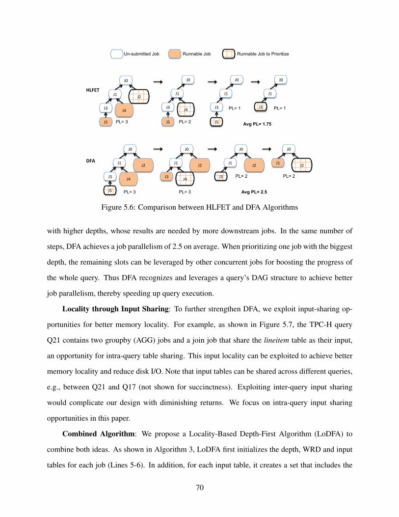
1
J1
J0
J2
J5
J4 J3
J1
J0
J5
J4 J3
J1
J0
J5
J3
J1
J0
J3
PL= 3 PL= 2
PL= 1 PL= 1
DFA
HLFET
Un-submitted Job Runnable Job Runnable Job to Prioritize
Avg PL= 1.75
Avg PL= 2.5
J1
J0
J2
J5
J4 J3
PL= 3
J1
J0
J2
J4 J3
PL= 3
J1
J0
J2 J1
J0
J2
J3 PL= 2 PL= 2
Figure 5.6: Comparison between HLFET and DFA Algorithms
with higher depths, whose results are needed by more downstream jobs. In the same number of
steps, DFA achieves a job parallelism of 2.5 on average. When prioritizing one job with the biggest
depth, the remaining slots can be leveraged by other concurrent jobs for boosting the progress of
the whole query. Thus DFA recognizes and leverages a query’s DAG structure to achieve better
job parallelism, thereby speeding up query execution.
Locality through Input Sharing: To further strengthen DFA, we exploit input-sharing op-
portunities for better memory locality. For example, as shown in Figure 5.7, the TPC-H query
Q21 contains two groupby (AGG) jobs and a join job that share the lineitem table as their input,
an opportunity for intra-query table sharing. This input locality can be exploited to achieve better
memory locality and reduce disk I/O. Note that input tables can be shared across different queries,
e.g., between Q21 and Q17 (not shown for succinctness). Exploiting inter-query input sharing
would complicate our design with diminishing returns. We focus on intra-query input sharing
opportunities in this paper.
Combined Algorithm: We propose a Locality-Based Depth-First Algorithm (LoDFA) to
combine both ideas. As shown in Algorithm 3, LoDFA first initializes the depth, WRD and input
tables for each job (Lines 5-6). In addition, for each input table, it creates a set that includes the
70
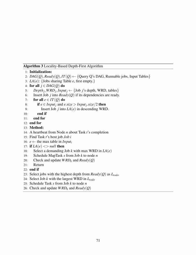
Algorithm 3 Locality-Based Depth-First Algorithm1: Initialization:2: DAG(Q),Ready(Q), IT (Q)← {Query Q’s DAG, Runnable jobs, Input Tables}3: LA(e): {Jobs sharing Table e, first empty.}4: for all j ∈ DAG(Q) do5: Depth j,WRD j, Input j← {Job j’s depth, WRD, tables}6: Insert Job j into Ready(Q) if its dependencies are ready.7: for all e ∈ IT (Q) do8: if e ∈ Input j and e.size > Input j.size/2 then9: Insert Job j into LA(e) in descending WRD.
10: end if11: end for12: end for13: Method:14: A heartbeat from Node n about Task t’s completion15: Find Task t’s host job Job i16: e← the max table in Inputi17: if LA(e)<> null then18: Select a demanding Job k with max WRD in LA(e)19: Schedule MapTask s from Job k to node n20: Check and update WRDk and Ready(Q)21: Return22: end if23: Select jobs with the highest depth from Ready(Q) as Ltodo24: Select Job k with the largest WRD in Ltodo25: Schedule Task s from Job k to node n26: Check and update WRDk and Ready(Q)
71
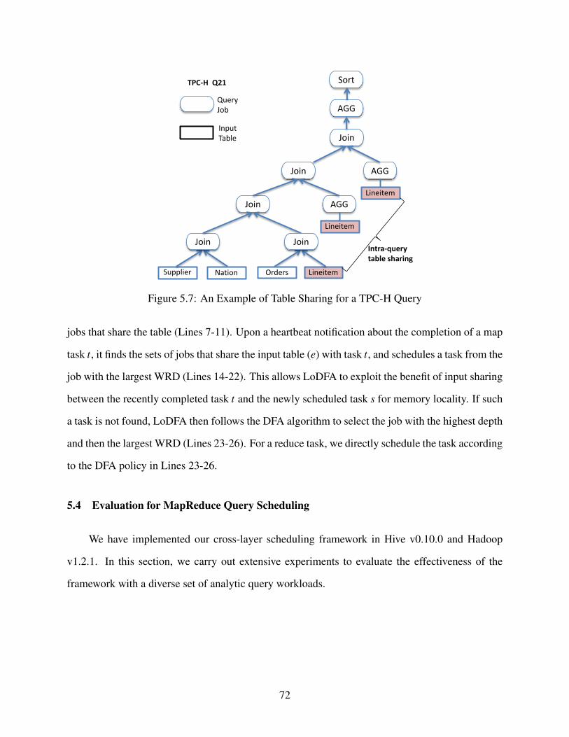
S-31
Supplier
TPC-H Q21
Query Job
Input Table
Join
Join AGG
Join AGG
Join
Nation Lineitem
Join
Orders
AGG
Lineitem
Lineitem
Intra-query table sharing
Sort
Figure 5.7: An Example of Table Sharing for a TPC-H Query
jobs that share the table (Lines 7-11). Upon a heartbeat notification about the completion of a map
task t, it finds the sets of jobs that share the input table (e) with task t, and schedules a task from the
job with the largest WRD (Lines 14-22). This allows LoDFA to exploit the benefit of input sharing
between the recently completed task t and the newly scheduled task s for memory locality. If such
a task is not found, LoDFA then follows the DFA algorithm to select the job with the highest depth
and then the largest WRD (Lines 23-26). For a reduce task, we directly schedule the task according
to the DFA policy in Lines 23-26.
5.4 Evaluation for MapReduce Query Scheduling
We have implemented our cross-layer scheduling framework in Hive v0.10.0 and Hadoop
v1.2.1. In this section, we carry out extensive experiments to evaluate the effectiveness of the
framework with a diverse set of analytic query workloads.
72
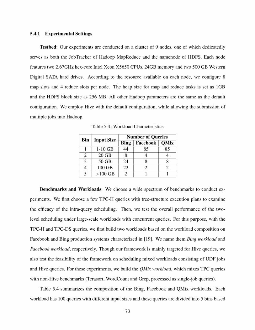
5.4.1 Experimental Settings
Testbed: Our experiments are conducted on a cluster of 9 nodes, one of which dedicatedly
serves as both the JobTracker of Hadoop MapReduce and the namenode of HDFS. Each node
features two 2.67GHz hex-core Intel Xeon X5650 CPUs, 24GB memory and two 500 GB Western
Digital SATA hard drives. According to the resource available on each node, we configure 8
map slots and 4 reduce slots per node. The heap size for map and reduce tasks is set as 1GB
and the HDFS block size as 256 MB. All other Hadoop parameters are the same as the default
configuration. We employ Hive with the default configuration, while allowing the submission of
multiple jobs into Hadoop.
Table 5.4: Workload Characteristics
Bin Input Size Number of QueriesBing Facebook QMix
1 1-10 GB 44 85 852 20 GB 8 4 43 50 GB 24 8 84 100 GB 22 2 25 >100 GB 2 1 1
Benchmarks and Workloads: We choose a wide spectrum of benchmarks to conduct ex-
periments. We first choose a few TPC-H queries with tree-structure execution plans to examine
the efficacy of the intra-query scheduling. Then, we test the overall performance of the two-
level scheduling under large-scale workloads with concurrent queries. For this purpose, with the
TPC-H and TPC-DS queries, we first build two workloads based on the workload composition on
Facebook and Bing production systems characterized in [19]. We name them Bing workload and
Facebook workload, respectively. Though our framework is mainly targeted for Hive queries, we
also test the feasibility of the framework on scheduling mixed workloads consisting of UDF jobs
and Hive queries. For these experiments, we build the QMix workload, which mixes TPC queries
with non-Hive benchmarks (Terasort, WordCount and Grep, processed as single-job queries).
Table 5.4 summarizes the composition of the Bing, Facebook and QMix workloads. Each
workload has 100 queries with different input sizes and these queries are divided into 5 bins based
73
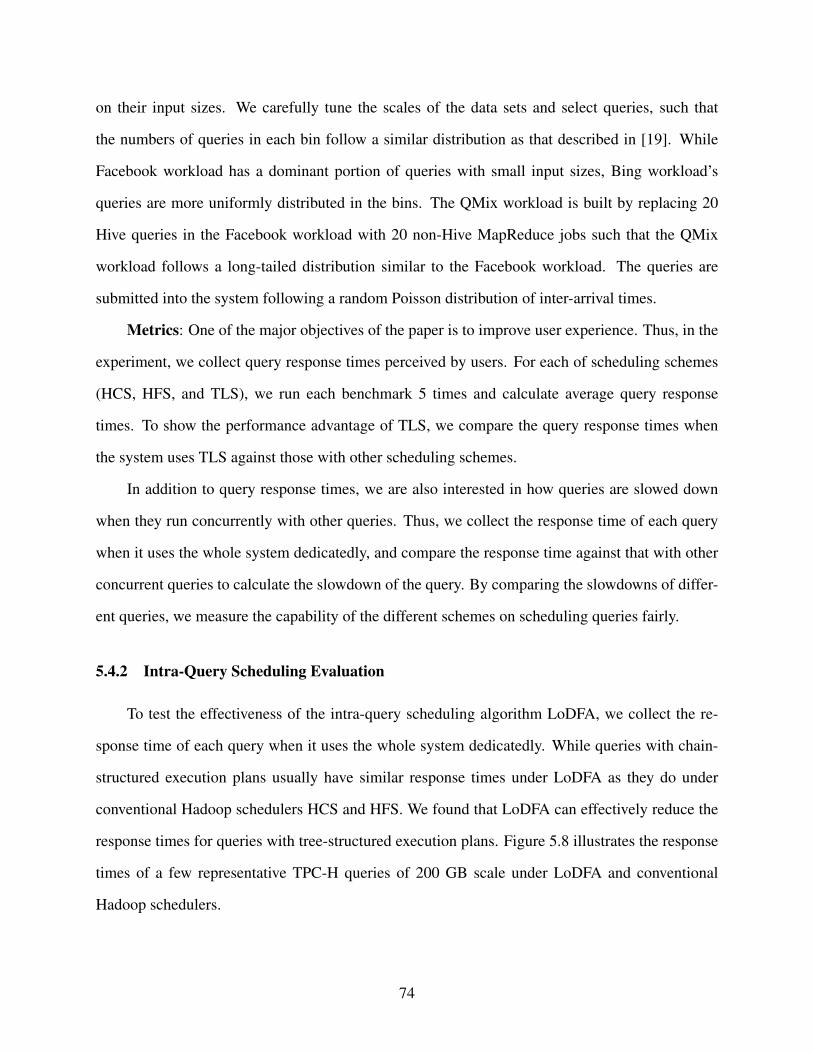
on their input sizes. We carefully tune the scales of the data sets and select queries, such that
the numbers of queries in each bin follow a similar distribution as that described in [19]. While
Facebook workload has a dominant portion of queries with small input sizes, Bing workload’s
queries are more uniformly distributed in the bins. The QMix workload is built by replacing 20
Hive queries in the Facebook workload with 20 non-Hive MapReduce jobs such that the QMix
workload follows a long-tailed distribution similar to the Facebook workload. The queries are
submitted into the system following a random Poisson distribution of inter-arrival times.
Metrics: One of the major objectives of the paper is to improve user experience. Thus, in the
experiment, we collect query response times perceived by users. For each of scheduling schemes
(HCS, HFS, and TLS), we run each benchmark 5 times and calculate average query response
times. To show the performance advantage of TLS, we compare the query response times when
the system uses TLS against those with other scheduling schemes.
In addition to query response times, we are also interested in how queries are slowed down
when they run concurrently with other queries. Thus, we collect the response time of each query
when it uses the whole system dedicatedly, and compare the response time against that with other
concurrent queries to calculate the slowdown of the query. By comparing the slowdowns of differ-
ent queries, we measure the capability of the different schemes on scheduling queries fairly.
5.4.2 Intra-Query Scheduling Evaluation
To test the effectiveness of the intra-query scheduling algorithm LoDFA, we collect the re-
sponse time of each query when it uses the whole system dedicatedly. While queries with chain-
structured execution plans usually have similar response times under LoDFA as they do under
conventional Hadoop schedulers HCS and HFS. We found that LoDFA can effectively reduce the
response times for queries with tree-structured execution plans. Figure 5.8 illustrates the response
times of a few representative TPC-H queries of 200 GB scale under LoDFA and conventional
Hadoop schedulers.
74
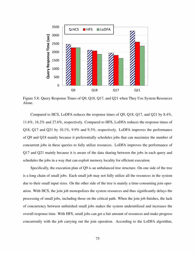
0
500
1000
1500
2000
2500
3000
3500
Q9 Q18 Q17 Q21
Qu
ery
Re
spo
nse
Tim
e (
sec)
HCS HFS LoDFA
Figure 5.8: Query Response Times of Q9, Q18, Q17, and Q21 when They Use System ResourcesAlone.
Compared to HCS, LoDFA reduces the response times of Q9, Q18, Q17, and Q21 by 8.4%,
11.6%, 16.2% and 27.6%, respectively. Compared to HFS, LoDFA reduces the response times of
Q18, Q17 and Q21 by 10.1%, 9.9% and 9.3%, respectively. LoDFA improves the performance
of Q9 and Q18 mainly because it preferentially schedules jobs that can maximize the number of
concurrent jobs in these queries to fully utilize resources. LoDFA improves the performance of
Q17 and Q21 mainly because it is aware of the data sharing between the jobs in each query and
schedules the jobs in a way that can exploit memory locality for efficient execution.
Specifically, the execution plan of Q9 is an unbalanced tree structure. On one side of the tree
is a long chain of small jobs. Each small job may not fully utilize all the resources in the system
due to their small input sizes. On the other side of the tree is mainly a time-consuming join oper-
ation. With HCS, the join job monopolizes the system resources and thus significantly delays the
processing of small jobs, including those on the critical path. When the join job finishes, the lack
of concurrency between unfinished small jobs makes the system underutilized and increases the
overall response time. With HFS, small jobs can get a fair amount of resources and make progress
concurrently with the job carrying out the join operation. According to the LoDFA algorithm,
75
small jobs on the long chain are preferentially scheduled according to the LoDFA algorithm. Thus,
HFS and LoDFA achieve better performance than HCS.
Q18 shows the performance advantage of DFA acquired by prioritizing the jobs with large
depths and WRDs. Usually, jobs with large depths and WRD are on critical paths and there are
other pending jobs depending on their results. Prioritizing these jobs reduces the delay to other
jobs and helps “releasing” more jobs to increase concurrency. Thus, LoDFA achieves better per-
formance than HCS and HFS.
Since in Q17 and Q21 the jobs on the leaf nodes of their execution plans share the same big
table (lineitem), the sharing-aware scheduling in LoDFA can consecutively execute the tasks of
jobs sharing the same data sets and improve data access’ temporal locality for these jobs. Such
strategy reduces the amount of data to be read from disks and accelerates the execution of map and
reduce tasks. Take Q17 as an example. When HCS is replaced by LoDFA, the data read from disks
is reduced by 37.1% in each of its execution. This translates to the 44.2% and 19% reductions of
the aggregated execution time for map operations and reduce operations respectively.
0
500
1000
1500
2000
2500
5G 10G 20G 50G 100G
Qu
ery
Re
spo
nse
Tim
e (
sec)
HCS HFS LoDFA
Figure 5.9: Query Response Times of 5 Instances of Q21 with Different Input Sizes.
When queries run concurrently and contend for resources, the intra-query scheduling algo-
rithm - LoDFA becomes more effective in reducing query response times, especially for small
76
queries. At the same time, it improves the data temporal locality among jobs that share data and
hence increases system throughput. To prevent the interferences from irrelevant factors, we submit
5 queries with the same query number (i.e. same execution plans) but with different input sizes
(from 5GB to 100GB) simultaneously to the system.
We measure and compare the response times of each query under different scheduling schemes.
The system throughput is determined by the response time of the query that finishes the last. Fig-
ure 5.9 shows the performance advantage of LoDFA over the two conventional Hadoop schedulers
for the queries with Q21. With HCS, five queries have similar response times. This is because the
executions of the queries with small inputs are significantly delayed by the jobs from the queries
with large inputs and the execution priority is turned around among all five queries. The HFS
scheduler ameliorates this situation. It shortens the response times of small queries at the cost of
slightly increased response time for the largest query (and the system throughput). Compared to
HFS, LoDFA further reduces the response times of small queries by large percentages (up to 61.8%
for the query with the input size of 5GB). In addition, LoDFA reduces the response time even for
the largest query, which also indicates the increase of the system throughput. Overall, LoDFA
on average reduces the response time by 34.2% and increases system throughput by 11.6% com-
pared with HFS. These improvements are mainly caused by the facts that TLS tends to increase
locality by not assigning resources in an interweaving manner among queries and LoDFA can ef-
fectively exploit the data-sharing opportunities among jobs. In doing so, we not only accelerate
the execution of each individual query, but also bring global benefits by reducing the contention
for resources.
5.4.3 Overall Performance
In this section, we use Bing, Facebook and QMix workloads to test the overall performance
of TLS. This evaluation helps us to understand how TLS performs under large-scale workloads,
in which different types of queries with a wide range of input sizes are submitted by multiple
independent users.
77
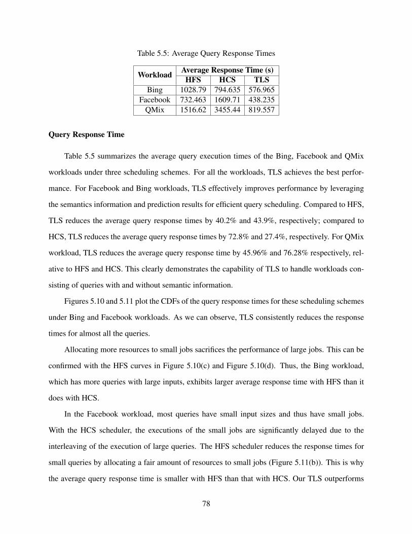
Table 5.5: Average Query Response Times
Workload Average Response Time (s)HFS HCS TLS
Bing 1028.79 794.635 576.965Facebook 732.463 1609.71 438.235
QMix 1516.62 3455.44 819.557
Query Response Time
Table 5.5 summarizes the average query execution times of the Bing, Facebook and QMix
workloads under three scheduling schemes. For all the workloads, TLS achieves the best perfor-
mance. For Facebook and Bing workloads, TLS effectively improves performance by leveraging
the semantics information and prediction results for efficient query scheduling. Compared to HFS,
TLS reduces the average query response times by 40.2% and 43.9%, respectively; compared to
HCS, TLS reduces the average query response times by 72.8% and 27.4%, respectively. For QMix
workload, TLS reduces the average query response time by 45.96% and 76.28% respectively, rel-
ative to HFS and HCS. This clearly demonstrates the capability of TLS to handle workloads con-
sisting of queries with and without semantic information.
Figures 5.10 and 5.11 plot the CDFs of the query response times for these scheduling schemes
under Bing and Facebook workloads. As we can observe, TLS consistently reduces the response
times for almost all the queries.
Allocating more resources to small jobs sacrifices the performance of large jobs. This can be
confirmed with the HFS curves in Figure 5.10(c) and Figure 5.10(d). Thus, the Bing workload,
which has more queries with large inputs, exhibits larger average response time with HFS than it
does with HCS.
In the Facebook workload, most queries have small input sizes and thus have small jobs.
With the HCS scheduler, the executions of the small jobs are significantly delayed due to the
interleaving of the execution of large queries. The HFS scheduler reduces the response times for
small queries by allocating a fair amount of resources to small jobs (Figure 5.11(b)). This is why
the average query response time is smaller with HFS than that with HCS. Our TLS outperforms
78
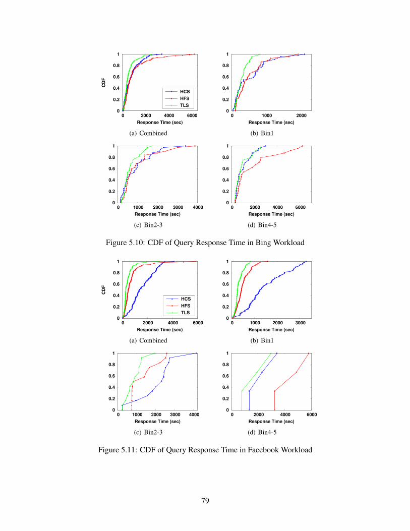
0
0.2
0.4
0.6
0.8
1
0 2000 4000 6000
CD
F
Response Time (sec)
HCS
HFS
TLS
(a) Combined
0
0.2
0.4
0.6
0.8
1
0 1000 2000
Response Time (sec)
(b) Bin1
0
0.2
0.4
0.6
0.8
1
0 1000 2000 3000 4000
Response Time (sec)
(c) Bin2-3
0
0.2
0.4
0.6
0.8
1
0 2000 4000 6000
Response Time (sec)
(d) Bin4-5
Figure 5.10: CDF of Query Response Time in Bing Workload
0
0.2
0.4
0.6
0.8
1
0 2000 4000 6000
CD
F
Response Time (sec)
HCS
HFS
TLS
(a) Combined
0
0.2
0.4
0.6
0.8
1
0 1000 2000 3000
Response Time (sec)
(b) Bin1
0
0.2
0.4
0.6
0.8
1
0 1000 2000 3000 4000
Response Time (sec)
(c) Bin2-3
0
0.2
0.4
0.6
0.8
1
0 2000 4000 6000
Response Time (sec)
(d) Bin4-5
Figure 5.11: CDF of Query Response Time in Facebook Workload
79
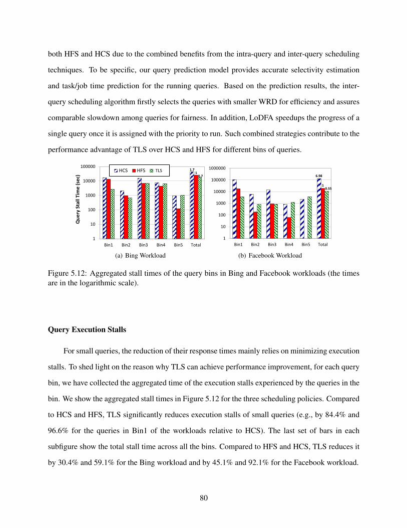
both HFS and HCS due to the combined benefits from the intra-query and inter-query scheduling
techniques. To be specific, our query prediction model provides accurate selectivity estimation
and task/job time prediction for the running queries. Based on the prediction results, the inter-
query scheduling algorithm firstly selects the queries with smaller WRD for efficiency and assures
comparable slowdown among queries for fairness. In addition, LoDFA speedups the progress of a
single query once it is assigned with the priority to run. Such combined strategies contribute to the
performance advantage of TLS over HCS and HFS for different bins of queries.
1
10
100
1000
10000
100000
Bin1 Bin2 Bin3 Bin4 Bin5 Total
Que
ry S
tall
Tim
e (s
ec)
HCS HFS Cross 1.71
0.7TLS
(a) Bing Workload
1
10
100
1000
10000
100000
1000000
Bin1 Bin2 Bin3 Bin4 Bin5 Total
6.98
0.55 1
(b) Facebook Workload
Figure 5.12: Aggregated stall times of the query bins in Bing and Facebook workloads (the timesare in the logarithmic scale).
Query Execution Stalls
For small queries, the reduction of their response times mainly relies on minimizing execution
stalls. To shed light on the reason why TLS can achieve performance improvement, for each query
bin, we have collected the aggregated time of the execution stalls experienced by the queries in the
bin. We show the aggregated stall times in Figure 5.12 for the three scheduling policies. Compared
to HCS and HFS, TLS significantly reduces execution stalls of small queries (e.g., by 84.4% and
96.6% for the queries in Bin1 of the workloads relative to HCS). The last set of bars in each
subfigure show the total stall time across all the bins. Compared to HFS and HCS, TLS reduces it
by 30.4% and 59.1% for the Bing workload and by 45.1% and 92.1% for the Facebook workload.
80
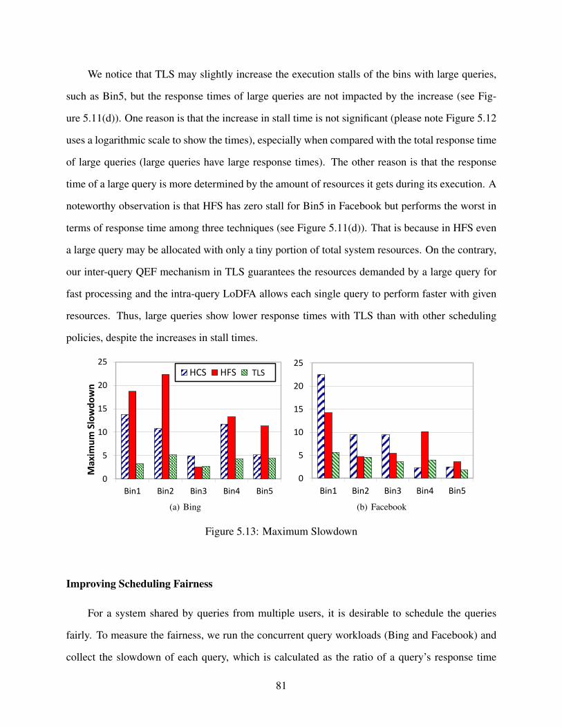
We notice that TLS may slightly increase the execution stalls of the bins with large queries,
such as Bin5, but the response times of large queries are not impacted by the increase (see Fig-
ure 5.11(d)). One reason is that the increase in stall time is not significant (please note Figure 5.12
uses a logarithmic scale to show the times), especially when compared with the total response time
of large queries (large queries have large response times). The other reason is that the response
time of a large query is more determined by the amount of resources it gets during its execution. A
noteworthy observation is that HFS has zero stall for Bin5 in Facebook but performs the worst in
terms of response time among three techniques (see Figure 5.11(d)). That is because in HFS even
a large query may be allocated with only a tiny portion of total system resources. On the contrary,
our inter-query QEF mechanism in TLS guarantees the resources demanded by a large query for
fast processing and the intra-query LoDFA allows each single query to perform faster with given
resources. Thus, large queries show lower response times with TLS than with other scheduling
policies, despite the increases in stall times.
0
5
10
15
20
25
Bin1 Bin2 Bin3 Bin4 Bin5
Max
imum
Slo
wdo
wn
HCS HFS CrossTLS
(a) Bing
0
5
10
15
20
25
Bin1 Bin2 Bin3 Bin4 Bin5
(b) Facebook
Figure 5.13: Maximum Slowdown
Improving Scheduling Fairness
For a system shared by queries from multiple users, it is desirable to schedule the queries
fairly. To measure the fairness, we run the concurrent query workloads (Bing and Facebook) and
collect the slowdown of each query, which is calculated as the ratio of a query’s response time
81
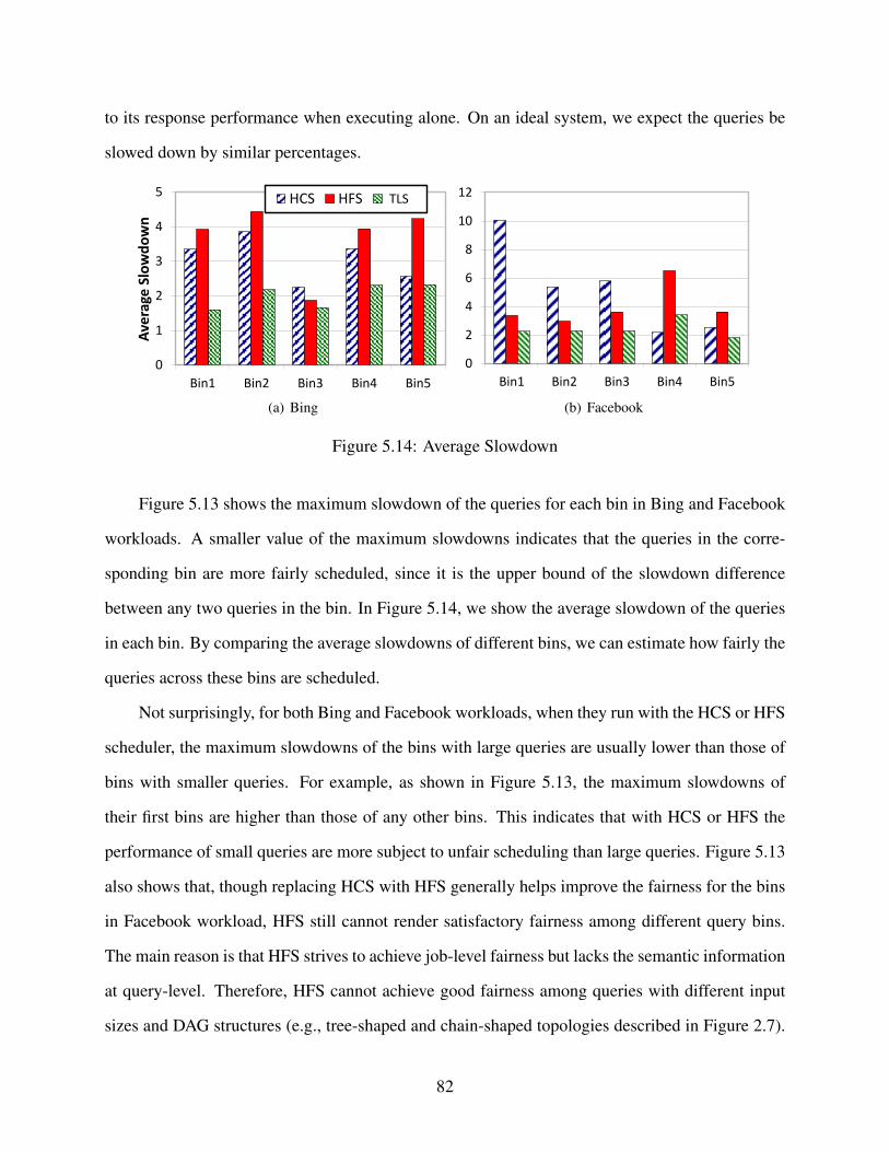
to its response performance when executing alone. On an ideal system, we expect the queries be
slowed down by similar percentages.
0
1
2
3
4
5
Bin1 Bin2 Bin3 Bin4 Bin5
Aver
age
Slow
dow
n
HCS HFS CrossTLS
(a) Bing
0
2
4
6
8
10
12
Bin1 Bin2 Bin3 Bin4 Bin5
(b) Facebook
Figure 5.14: Average Slowdown
Figure 5.13 shows the maximum slowdown of the queries for each bin in Bing and Facebook
workloads. A smaller value of the maximum slowdowns indicates that the queries in the corre-
sponding bin are more fairly scheduled, since it is the upper bound of the slowdown difference
between any two queries in the bin. In Figure 5.14, we show the average slowdown of the queries
in each bin. By comparing the average slowdowns of different bins, we can estimate how fairly the
queries across these bins are scheduled.
Not surprisingly, for both Bing and Facebook workloads, when they run with the HCS or HFS
scheduler, the maximum slowdowns of the bins with large queries are usually lower than those of
bins with smaller queries. For example, as shown in Figure 5.13, the maximum slowdowns of
their first bins are higher than those of any other bins. This indicates that with HCS or HFS the
performance of small queries are more subject to unfair scheduling than large queries. Figure 5.13
also shows that, though replacing HCS with HFS generally helps improve the fairness for the bins
in Facebook workload, HFS still cannot render satisfactory fairness among different query bins.
The main reason is that HFS strives to achieve job-level fairness but lacks the semantic information
at query-level. Therefore, HFS cannot achieve good fairness among queries with different input
sizes and DAG structures (e.g., tree-shaped and chain-shaped topologies described in Figure 2.7).
82
However, TLS achieves much lower maximum slowdowns for all the bins than HCS and HFS.
This confirms that TLS can improve fairness significantly and consistently, irrespective of the
query input sizes.
As shown in Figure 5.14, with HCS, small queries are biased by the scheduler, and they
are usually slowed down by higher percentages than large queries. For example, for the Facebook
workload, HCS incurs 10.1× average slowdown for the queries in Bin1 but 2.5× for Bin5. Though
HFS may improve the fairness, the improvement comes at the cost of the performance of large
queries. For example, compared to HCS, HFS significantly increases the average slowdowns of
Bin4 and Bin5 in the Facebook workload. However, TLS can improve fairness more effectively
than HFS. With TLS, the average slowdowns of different bins show much smaller variations than
those with HFS. More importantly, the better fairness comes without degrading the performance.
For all the bins, the average slowdowns are much lower than those with either HFS or HCS.
5.5 Related Studies on MapReduce and Scheduling
In this section, we review recent work on query modeling and scheduling in the MapReduce
environment.
5.5.1 Query Modeling
Morton et al. [68] proposed the Paratimer model to estimate the progress of Pig queries,
which are translated into DAGs of MapReduce jobs. Their model incorporated dataset cardinality
and unit processing time. Verma et al. [100, 121] provided a “work/speed” time model for the
relationship of execution time and available resources. Both time models require pre-execution
profiling or debug runs of the same job in order to acquire the necessary phase information to
estimate the job’s execution time. Our work leverages selectivity estimation and does not require
such pre-execution or debug runs of MapReduce queries.
In [69], Mullin proposed a partial bloom filter based join selectivity estimation algorithm. In
[21], Bell et. al presented a piece-wise uniform approach for estimating the frequency distribution
83
of join attributes by equal-width histograms. In [30], Dell’aquila exploited the canonical coefficient
parameters of estimating selectivity factors for relational operations through approximating both
the multivariate data distribution and distinct values of attributes. Swami et al. [91] attempted
selectivity prediction for multi-join operations with a common key and uniform key distribution.
Our work extends this prior study to provide selectivity prediction for multi-join operations on
different keys with piece-wise uniform distribution in the MapReduce environment.
Wu et al. [111] proposed AQUA as a comprehensive cost model to estimate CPU, network
and I/O costs of database operations and MapReduce jobs. Our work is different from AQUA as a
time based model and includes selectivity estimation for different types of query jobs. Li et al. [59]
estimated query’s resource demands using statistical models for individual operators of database
queries. Ganapathi et al. [38, 37] developed a KCCA (Kernel Canonical Correlation Analysis)
model based prediction system to solve the database query time estimation. Compared to these
studies, we design a multivariate model for queries in MapReduce-based data warehouse systems.
5.5.2 MapReduce Scheduling and Other Related Work
Algorithms for scheduling jobs and/or DAGs of jobs have been studied based on general
models. For example, the Johnson’s algorithm [49] was proposed to solve two- and three-stage
Job-shop problems. HLFET was proposed by Adam et al. [17] as a scheduling algorithm for DAGs
of jobs in a multiprocessor environment. Similarly, Hu et al. [43] proposed a polynomial schedule
algorithm for in-tree structured DAGs with unit computation cost. These algorithms cannot be
directly applied to schedule analytic Hive queries due to the special features of Hive queries and
frameworks. For example, Johnson’s algorithm is not applicable for query scheduling due to the
precedence constraint of jobs. In addition, parallelism level in MapReduce environment is flexible
and job nodes in the query DAG are of non-uniform costs, which are different from the scenarios
in [17] and [43].
84
Targeting the scheduling of individual MapReduce jobs, various algorithms were proposed.
For example, Zaharia et al. [118] proposed delay scheduling to promote data locality in the schedul-
ing of MapReduce jobs. Wolf et al. proposed a malleable scheduler Flex for optimizing the min-
isum and minimax metrics of response time, stretch, deadlines, etc [108]. They are not aware of
the relationship of jobs in a DAG.
In some runtime engines (e.g. Spark [119], Dryad [46], Tez [3]), the structures of DAGs are
considered. Shenker et al. [85] implemented Shark as a scalable SQL and Rich Analytics on top of
Spark. Yu et al. [117] designed the DryadLINQ model for users to conduct declarative operations
on distributed datasets. A DryadLINQ program is translated into an execution plan graph where
each vertex is to execute as a Dryad job on the cluster-computing infrastructure. Ke et al. [50]
provided a framework called Optimus for dynamically rewriting EPG (Execution Plan Graph) at
runtime in DryadLINQ. Their work focuses on rewriting the upper-layer query plan by analyzing
real-time statistics passed from low-layer runtime. Compared to these studies, our work leverages
semantic information from DAG queries for modeling of job execution time and then employs the
model into our two-level scheduler to improve scheduling efficiency.
Recently, FlowFlex extended the Flex scheduler to schedule flows (i.e. DAGs) of MapReduce
jobs [70]. It provides a theoretic study and assumes the scheduler already know the amount of
work in each job. TLS provides a whole package of solution from job execution time prediction
and scheduling algorithms to real implementation. It is also based on richer semantic information,
which is used to exploit more performance optimization opportunities. Tez [3] was developed for
accelerating query processing in Hive/Hadoop. It supports DAG and task scheduling for every
query and adopts a simplistic scheme for determining vertex priority and task parallelism of each
vertex. However, it cannot estimate the execution times of the each node and query, and thus cannot
correctly identify and schedule vertices on critical execution paths. Specifically, Tez allocates
resources randomly among leaf nodes (runnable vertices) in each DAG and treats queries equally,
in spite of their large differences in term of resource demands.
85
5.6 Summary
Many popular data warehouse systems are deployed on top of MapReduce. Complex ana-
lytic queries are usually compiled into directed acyclic graphs (DAGs). However, the simplistic
job-level scheduling policy in MapReduce is unable to balance resource distribution and reconcile
the dynamic needs of different jobs in DAGs. To address such issues systematically, we develop
a scheduling framework which includes two main techniques: multivariate DAG modeling and
two-level scheduling. Multivariate DAG modeling can accurately predict the changing data sizes
and the execution time of jobs in DAG queries. Two-level scheduling is designed to allocate re-
sources and schedule tasks at both inter-query and intra-query levels for efficient and fair execution
of concurrent queries. The multivariate model offers important inputs for scheduling decisions in
our two-level scheduler. Experiment results demonstrate that our techniques can achieve steady
performance improvement over traditional scheduling techniques for representative query bench-
marks due to accurate query time estimation, efficient resource allocation and reduced execution
stalls. Furthermore, our two-level scheduler also significantly enhances query fairness.
86
Chapter 6
Conclusion
The dissertation investigates the big data challenges from two major perspectives: first, how
to enable applications with fast data retrieval to storage systems; second, how to analyze big data
efficiently. To tackle these challenges, I have invested substantial efforts in devising fast PCM-
based hybrid storage system and optimizing I/O performance of scientific applications for fast
data retrial; and developing a prediction-based scheduling framework on MapReduce-based data
warehouse system for efficient data analytics. To this end, this dissertation has made the following
three key contributions for addressing big data challenges.
In order to improve the big data storage and retrieval, I devise a PCM-Based Hybrid Storage
System to improve I/O performance for traditional hard disk based storage system in Chapter 3.
This hybrid storage system involves a novel write cache mapping and management scheme and two
wear leveling algorithms for prolonging the life time of phase change memory. The HALO caching
scheme introduces an efficient mapping and indexing schemes using advanced data structures such
as bucket-based hashing and cuckoo hash table; in addition, a two-way destaging scheme is devised
for data spatial and temporal locality optimization. As a result, HALO caching guarantees data
reliability and greatly speeds up the I/O performance of diversified workloads (on average, 36.8%).
The two novel wear leveling algorithms refer to rank-bank round-robin wear leveling and space
filling curve based wear leveling, which prolong the PCM’s life time by as much as 21.6 times.
In order to boost data access performance of scientific applications, we profile and address
influential factors that can prevent current scientific applications from achieving efficient I/O of
underlying parallel storage systems in Chapter 4. Particularly, we select a mission-critical appli-
cation NASA GEOS-5 climate modeling as our case study. Through comprehensive experimental
dissection and analysis, we observe that the hierarchical data aggregation and I/O patterns existent
87
in legacy applications can cause redundant network traffic and serious single-point contention is-
sues. Therefore, we have modified GEOS-5’s current I/O frameworks and enabled the application
to exploits the benefits from the state-of-art parallel I/O interfaces such as PnetCDF and ADIOS.
Experimental results on the NASA discover cluster shows that our technique can consistently im-
prove the I/O performance of GEOS-5 for at various scales because of the elimination of redundant
network aggregation and greatly promoted I/O concurrency.
In order to optimize the big data analytics, I identify the efficiency and fairness problems re-
siding in current MapReduce schedulers and develop a prediction-based two-level query schedul-
ing framework on Hive and Hadoop in Chapter 5. This framework is leveraged for bridging the
semantic gap between Hive and Hadoop, conducting accurate resource usage and time estimation
of queries, and enabling efficient two-level query scheduling for optimal fairness and response
performance among concurrent analytic queries. Specifically, first the multivariate DAG model-
ing can accurately predict the changing data sizes and the execution time of jobs in DAG queries.
Then, based on the predicted information, the two-level query scheduling is proposed to allocate
resources and schedule tasks at both inter-query and intra-query levels for efficient and fair execu-
tion of concurrent queries. Experiment results demonstrate that our framework can achieve accu-
rate query estimation and significant efficient and fairness improvement over traditional scheduling
techniques for representative query benchmarks.
88
Chapter 7
Future Plan
In this chapter, we discuss some related ideas and topics that can further optimize and extend
our accomplished work in different aspects. These issues can help create to a series of opportunities
which we will investigate in our future studies.
PCM and storage system: we plan to study dynamically partitioned read/write cache schemes
for improving a wider range of workload patterns. Particularly, a workload-aware prefetching
scheme can be introduced for expediting the read response performance. In addition, an efficient
PCM space management and allocation scheme is also in need. For further reducing memory
overhead of cache mapping, a scalable and hierarchical hash table can be introduced. In terms of
endurance, we have thought of another critical issue existing in current NVM wear leveling algo-
rithms, namely, the row buffer locality that might be destroyed by the randomized mapping and
cache line rotation introduced in traditional wear leveling algorithms such as Start-Gap [77]. Cor-
respondingly, we are designing a bijective-matrix based mapping scheme and a row buffer locality
aware rotation algorithm for achieving endurance without sacrificing memory performance.
Application I/O Optimization: it is of good potential to study asynchronous I/O schemes and
efficient burst buffering techniques for further I/O performance improvements of scientific appli-
cations. To be specific, non-volatile memory technologies such as PCM or FSSD can be integrated
into the storage hierarchy of traditional parallel storage systems such as Lustre. Furthermore, our
HALO caching and destaging schemes can be adapted to work in cooperation with upper-layer I/O
optimization framework for further boosting data depositing and retrieval performance of large-
scale applications.
89

Query scheduling and MapReduce: Recently, Hadoop ecosystem has evolved to version 2.0
- YARN (Yet Another Resource Negotiator) [99]. Therefore, I have just ported my query schedul-
ing framework also to YARN platform. The preliminary results demonstrate that our implemen-
tation can also improve query performance significantly compared to traditional scheduling algo-
rithms. In addition, we plan to extend the query prediction model as an accurate real-time query
progress indicator with concurrency, data skew and task failure considered. Such optimization
can not only provide expectable quality-of-service for users’ interactive requests, but also enable
the resource scheduler to determine the possible deadline of each request for SLA (Service Level
Agreement). Currently the low-latency interactive data processing engines such as Spark [119]
and streaming data processing engines such as Storm [2] have sprung up. It is very promising and
urgent for us to conduct accurate query resource estimation and smart resource scheduling for such
new data analytics paradigms.
90
Bibliography
[1] Adaptable I/O System. http://www.nccs.gov/user-support/center-projects/adios .
[2] Apache Storm. https://storm.apache.org/.
[3] Apache Tez. http://hortonworks.com/hadoop/tez/.
[4] Are hybrid drives finally coming of age? http://www.researchandmarkets.com/reports/1409321/are_hybrid_drives_finally_coming_of_age.pdf.
[5] Energy Sources. http://energy.gov/science-innovation/energy-sources.
[6] Micron phase change memory. http://www.micron.com/products/phase-change-memory.
[7] NASA Discover. http://www.nccs.nasa.gov/cluster main.html.
[8] NASA GEOS. http://gmao.gsfc.nasa.gov/systems/geos5.
[9] NETCDF. http://www.unidata.ucar.edu/software/netcdf.
[10] NVIDIA Tesla. http://www.nvidia.com/object/tesla-supercomputing\newline-solutions.html.
[11] The Parallel Virtual File System, version 2. http://www.pvfs.org/pvfs2.
[12] Top 500 supercomputing sites. http://www.top500.org.
[13] TPC. http://www.tpc.org/.
[14] Umass trace repository. http://traces.cs.umass.edu/.
[15] SNIA BlockIO Traces. http://iotta.snia.org/tracetypes/3, Online, 2006.
[16] H. Abbasi, M. Wolf, G. Eisenhauer, S. Klasky, K. Schwan, and F. Zheng. Datastager:scalable data staging services for petascale applications. In Proceedings of the 18th ACMinternational symposium on High performance distributed computing, HPDC ’09, pages39–48, New York, NY, USA, 2009. ACM.
[17] Thomas L Adam, K. Mani Chandy, and JR Dickson. A comparison of list schedules forparallel processing systems. Communications of the ACM, 17(12):685–690, 1974.
[18] A. Akel, A.M. Caulfield, T.I. Mollov, R.K. Gupta, and S. Swanson. Onyx: A prototypephase change memory storage array. In HotStorage’11.
91
[19] Ganesh Ananthanarayanan, Ali Ghodsi, Andrew Wang, Dhruba Borthakur, Srikanth Kan-dula, Scott Shenker, and Ion Stoica. Pacman: Coordinated memory caching for paralleljobs. In USENIX NSDI, 2012.
[20] M. Baker, S. Asami, E. Deprit, J. Ouseterhout, and M. Seltzer. Non-volatile memory forfast, reliable file systems. ACM SIGPLAN Notices, 27(9):10–22, 1992.
[21] David A Bell, DHO Link, and S McClean. Pragmatic estimation of join sizes and attributecorrelations. In ICDE, pages 76–84. IEEE, 1989.
[22] J. Bent, G. A. Gibson, G. Grider, B. McClelland, P. Nowoczynski, J. Nunez, M. Polte, andM. Wingate. PLFS: a checkpoint filesystem for parallel applications. In SC ’09: Proceed-ings of the Conference on High Performance Computing Networking, Storage and Analysis,2009.
[23] Alan D Brunelle. Blktrace user guide, 2007.
[24] John S. Bucy and G. R. Ganger. Technical report. http://www.pdl.cmu.edu/DiskSim/.
[25] Z. Liu H. Chen B. Neitzel C. Xu, R. Goldsone and W. Yu. Exploiting analytics shipping withvirtualized mapreduce on hpc backend storage servers. Parallel and Distributed Computing,IEEE Transactions on, 2015.
[26] S. Chen, P.B. Gibbons, and S. Nath. Rethinking database algorithms for phase changememory. CIDR11, pages 21–31, 2011.
[27] A. Choudhary, W. Liao, K. Gao, A. Nisar, R. Ross, R. Thakur, and R. Latham. Scalable I/Oand analytics. Journal of Physics, 180(1), 2009.
[28] Cluster File System, Inc. Lustre: A Scalable, High Performance File System. http://www.lustre.org/docs.html.
[29] Jeffrey Dean and Sanjay Ghemawat. Mapreduce: simplified data processing on large clus-ters. Communications of the ACM, 51(1):107–113, 2008.
[30] Carlo Dellaquila, Ezio Lefons, and Filippo Tangorra. Analytic-based estimation of queryresult sizes. In Proceedings of the 4th WSEAS International Conference on Artificial Intel-ligence, Knowledge Engineering Data Bases, page 24. WSEAS, 2005.
[31] X. Ding, S. Jiang, F. Chen, K. Davis, and X. Zhang. Diskseen: exploiting disk layout andaccess history to enhance i/o prefetch. In USENIX ATC, 2007.
[32] I.H. Doh, J. Choi, D. Lee, and S.H. Noh. Exploiting non-volatile ram to enhance flash filesystem performance. In ACM EMSOFT’07.
[33] I.H. Doh, H.J. Lee, Y.J. Moon, E. Kim, J. Choi, D. Lee, and S.H. Noh. Impact of nvramwrite cache for file system metadata on i/o performance in embedded systems. In ACMSAC’09.
92
[34] Jennie Duggan, Ugur Cetintemel, Olga Papaemmanouil, and Eli Upfal. Performance pre-diction for concurrent database workloads. In Proceedings of the 2011 ACM SIGMODInternational Conference on Management of data, pages 337–348. ACM, 2011.
[35] M. R. Fahey, J. M. Larkin, and J. Adams. I/O performance on a massively parallel crayXT3/XT4. In Proc. 22nd IEEE International Symposium on Parallel and Distributed Pro-cessing (22nd IPDPS’08), 2008.
[36] D. Fotakis, R. Pagh, P. Sanders, and P. Spirakis. Space efficient hash tables with worst caseconstant access time. STACS 2003, pages 271–282, 2003.
[37] Archana Ganapathi, Yanpei Chen, Armando Fox, Randy Katz, and David Patterson.Statistics-driven workload modeling for the cloud. In ICDEW. IEEE, 2010.
[38] Archana Ganapathi, Harumi Kuno, Umeshwar Dayal, Janet L Wiener, Armando Fox,Michael Jordan, and David Patterson. Predicting multiple metrics for queries: Better de-cisions enabled by machine learning. In Data Engineering, 2009. ICDE’09. IEEE 25thInternational Conference on, pages 592–603. IEEE, 2009.
[39] John Gantz and David Reinsel. The digital universe in 2020: Big data, bigger digital shad-ows, and biggest growth in the far east. IDC iView: IDC Analyze the Future, 2012.
[40] Alan F Gates, Olga Natkovich, Shubham Chopra, Pradeep Kamath, Shravan M Narayana-murthy, Christopher Olston, Benjamin Reed, Santhosh Srinivasan, and Utkarsh Srivastava.Building a high-level dataflow system on top of map-reduce: the pig experience. Proceed-ings of the VLDB Endowment, 2(2):1414–1425, 2009.
[41] B.S. Gill and D.S. Modha. Wow: wise ordering for writes-combining spatial and temporallocality in non-volatile caches. In USENIX FAST’05.
[42] C. Hill, C. DeLuca, V. Balaji, M. Suarez, and A. D. Silva. The architecture of the earthsystem modeling framework. Computing in Science and Engg., 6(1):18–28, January 2004.
[43] Te C Hu. Parallel sequencing and assembly line problems. Operations research, 9(6):841–848, 1961.
[44] J. H. Laros III, L. Ward, R. Klundt, S. Kelly, J. L. Tomkins, and B. R. Kellogg. Red stormIO performance analysis. In CLUSTER, 2007.
[45] E. Ipek, J. Condit, E. B. Nightingale, D. Burger, and T. Moscibroda. Dynamically replicatedmemory: building reliable systems from nanoscale resistive memories. ASPLOS’10.
[46] Michael Isard, Mihai Budiu, Yuan Yu, Andrew Birrell, and Dennis Fetterly. Dryad: dis-tributed data-parallel programs from sequential building blocks. ACM SIGOPS OperatingSystems Review, 41(3):59–72, 2007.
[47] S. Jiang, X. Ding, F. Chen, E. Tan, and X. Zhang. Dulo: an effective buffer cache manage-ment scheme to exploit both temporal and spatial locality. In USENIX FAST’05.
93
[48] S. Jiang and X. Zhang. Lirs: an efficient low inter-reference recency set replacement pol-icy to improve buffer cache performance. In ACM SIGMETRICS Performance EvaluationReview, volume 30, pages 31–42. ACM, 2002.
[49] Selmer Martin Johnson. Optimal two-and three-stage production schedules with setup timesincluded. Naval research logistics quarterly, 1(1):61–68, 1954.
[50] Qifa Ke, Michael Isard, and Yuan Yu. Optimus: a dynamic rewriting framework for data-parallel execution plans. In Proceedings of the 8th ACM European Conference on ComputerSystems, pages 15–28. ACM, 2013.
[51] J Keilson and LD Servi. A distributional form of little’s law. Operations Research Letters,7(5):223–227, 1988.
[52] C.S. Kim. Lrfu: A spectrum of policies that subsumes the least recently used and leastfrequently used policies. IEEE Transactions on Computers, 50(12), 2001.
[53] S. Lang, P. H. Carns, R. Latham, R. B. Ross, K. Harms, and W. E. Allcock. I/O performancechallenges at leadership scale. In SC’09 USB Key. ACM/IEEE, Portland, OR, USA, nov2009.
[54] Eunji Lee, Hyokyung Bahn, and Sam H Noh. Unioning of the buffer cache and journalinglayers with non-volatile memory. In FAST, pages 73–80. USENIX, 2013.
[55] KH Lee, IH Doh, J. Choi, D. Lee, and SH Noh. Write-aware buffer cache managementscheme for nonvolatile ram. In Proceedings of Advances in Computer Science and Technol-ogy. ACTA Press, 2007.
[56] Rubao Lee, Tian Luo, Yin Huai, Fusheng Wang, Yongqiang He, and Xiaodong Zhang. Ys-mart: Yet another sql-to-mapreduce translator. In Distributed Computing Systems (ICDCS),2011 31st International Conference on, pages 25–36. IEEE, 2011.
[57] D. Li, J. Vetter, G. Marin, C. McCurdy, C. Cira, Z. Liu, and W. Yu. Identifying opportu-nities for byte-addressable non-volatile memory in extreme-scale scientific applications. InIPDPS. IEEE, 2012.
[58] J. Li, W. Liao, A. Choudhary, R. Ross, R. Thakur, W. Gropp, and R. Latham. ParallelnetCDF: A High Performance Scientific I/O Interface. In Proc. SC03, 2003.
[59] Jiexing Li, Arnd Christian Konig, Vivek Narasayya, and Surajit Chaudhuri. Robust estima-tion of resource consumption for sql queries using statistical techniques. Proceedings of theVLDB Endowment, 5(11):1555–1566, 2012.
[60] Xian Liu and G.F. Schrack. An algorithm for encoding and decoding the 3-d hilbert order.Image Processing, IEEE Transactions on, 6(9):1333–1337, sep 1997.
[61] Z. Liu, B. Wang, P. Carpenter, D. Li, J. S. Vetter, and W. Yu. PCM-based durable write cachefor fast disk I/O. In Modeling, Analysis & Simulation of Computer and TelecommunicationSystems (MASCOTS), 2012 IEEE 20th International Symposium on, pages 451–458. IEEE,2012.
94
[62] Zhuo Liu, Jay Lofstead, Teng Wang, and Weikuan Yu. A case of system-wide power man-agement for scientific applications. In Cluster Computing (CLUSTER), 2013 IEEE Interna-tional Conference on, pages 1–8. IEEE, 2013.
[63] Zhuo Liu, Bin Wang, Teng Wang, Yuan Tian, Cong Xu, Yandong Wang, Weikuan Yu, Car-los A Cruz, Shujia Zhou, Tom Clune, and Scott Klasky. Profiling and improving i/o per-formance of a large-scale climate scientific application. In Computer Communications andNetworks (ICCCN), 2013 22nd International Conference on, pages 1–7. IEEE, 2013.
[64] Zhuo Liu, Jian Zhou, Weikuan Yu, Fei Wu, Xiao Qin, and Changsheng Xie. Mind: Ablack-box energy consumption model for disk arrays. In Green Computing Conference andWorkshops (IGCC), 2011 International, pages 1–6. IEEE, 2011.
[65] J. Lofstead, M. Polte, G. Gibson, S. Klasky, K. Schwan, R Oldfield, M. Wolf, and Q. Liu. Sixdegrees of scientific data: Reading patterns for extreme scale science io. In In Proceedingsof High Performance and Distributed Computing, 2011.
[66] J. Lofstead, F. Zheng, S. Klasky, and K. Schwan. Adaptable, metadata rich IO methods forportable high performance IO. In IPDPS’09, 2009.
[67] The HDF Group. Hierarchical data format version 5, 2000–2010.http://www.hdfgroup.org/HDF5.
[68] Kristi Morton, Magdalena Balazinska, and Dan Grossman. Paratimer: a progress indicatorfor mapreduce dags. In Proceedings of the 2010 ACM SIGMOD International Conferenceon Management of data, pages 507–518. ACM, 2010.
[69] James K Mullin. Estimating the size of a relational join. Information Systems, 18(3):189–196, 1993.
[70] Viswanath Nagarajan, Joel Wolf, Andrey Balmin, and Kirsten Hildrum. Flowflex: Malleablescheduling for flows of mapreduce jobs. In Middleware 2013, pages 103–122. Springer,2013.
[71] T. Nightingale, Y. Hu, and Q. Yang. The design and implementation of a dcd device driverfor unix. In USENIX ATC’99.
[72] E.J. O’neil, P.E. O’neil, and G. Weikum. The lru-k page replacement algorithm for databasedisk buffering. In ACM SIGMOD’93.
[73] OSDL. Iometer project. http://www.iometer.org/, Online, 2004.
[74] R. Pagh and F. Rodler. Cuckoo hashing. AlgorithmsESA 2001, pages 121–133, 2001.
[75] Y. Park, S.H. Lim, C. Lee, and K.H. Park. Pffs: a scalable flash memory file system for thehybrid architecture of phase-change ram and nand flash. In ACM SAC’08.
[76] Gregory Piatetsky-Shapiro and Charles Connell. Accurate estimation of the number oftuples satisfying a condition. In ACM SIGMOD Record, volume 14, pages 256–276. ACM,1984.
95
[77] M.K. Qureshi, J. Karidis, M. Franceschini, V. Srinivasan, L. Lastras, and B. Abali. En-hancing lifetime and security of pcm-based main memory with start-gap wear leveling. InIEEE/ACM Micro’09.
[78] M.K. Qureshi, V. Srinivasan, and J.A. Rivers. Scalable high performance main memorysystem using phase-change memory technology. In ISCA’09.
[79] L.E. Ramos, E. Gorbatov, and R. Bianchini. Page placement in hybrid memory systems. InICS’11.
[80] M. Rosenblum and J.K. Ousterhout. The design and implementation of a log-structured filesystem. ACM SIGOPS Operating Systems Review, 25(5):1–15, 1991.
[81] S. Saini, J. Rappleye, J. Chang, D.P. Barker, R. Biswas, and P. Mehrotra. I/O PerformanceCharacterization of Lustre and NASA Applications on Pleiades. In HiPC, 2012.
[82] S. W. Schlosser, J. Schindler, S. Papadomanolakis, M. Shao, A. Ailamaki, C. Faloutsos, andG. R. Ganger. On Multidimensional Data and Modern Disks. In FAST, 2005.
[83] F. Schmuck and R. Haskin. GPFS: A Shared-Disk File System for Large Computing Clus-ters. In FAST ’02, pages 231–244. USENIX, January 2002.
[84] Nak Hee Seong, Dong Hyuk Woo, and Hsien-Hsin S. Lee. Security refresh: prevent mali-cious wear-out and increase durability for phase-change memory with dynamically random-ized address mapping. In ISCA’10.
[85] Scott Shenker, Ion Stoica, Matei Zaharia, Reynold Xin, Josh Rosen, and Michael J Franklin.Shark: Sql and rich analytics at scale. In Proceedings of the 2013 ACM SIGMOD Interna-tional Conference on Management of Data, 2013.
[86] Liang Shi, Jianhua Li, Chun Jason Xue, and Xuehai Zhou. Hybrid nonvolatile disk cache forenergy-efficient and high-performance systems. ACM Transactions on Design Automationof Electronic Systems (TODAES), 18(1):8, 2013.
[87] T. Shimada, T. Tsuji, and K. Higuchi. A storage scheme for multidimensional data alleviat-ing dimension dependency. In Digital Information Management, 2008. ICDIM 2008. ThirdInternational Conference on, 2008.
[88] Gokul Soundararajan, Vijayan Prabhakaran, Mahesh Balakrishnan, and Ted Wobber. Ex-tending ssd lifetimes with disk-based write caches. In USENIX FAST’10.
[89] M. Suarez, A. Trayanov, C. Hill, P. Schopf, and Y. Vikhliaev. MAPL: a high-level program-ming paradigm to support more rapid and robust encoding of hierarchical trees of interactinghigh-performance components. In Proceedings of the 2007 symposium on Component andframework technology in high-performance and scientific computing, 2007.
[90] G. Sun, Y. Joo, Y. Chen, D. Niu, Y. Xie, Y. Chen, and H. Li. A hybrid solid-state storagearchitecture for the performance, energy consumption, and lifetime improvement. In IEEEHPCA’10.
96
[91] A. Swami and K.B. Schiefer. On the estimation of join result sizes. IBM Technical Report,1993.
[92] Jian Tan, Xiaoqiao Meng, and Li Zhang. Delay tails in mapreduce scheduling. In Pro-ceedings of the 12th ACM SIGMETRICS/PERFORMANCE joint international conferenceon Measurement and Modeling of Computer Systems, SIGMETRICS ’12, pages 5–16, NewYork, NY, USA, 2012. ACM.
[93] The National Center for SuperComputing. HDF Home Page. http://hdf.ncsa.uiuc.com/hdf4.html.
[94] Ashish Thusoo, Joydeep Sen Sarma, Namit Jain, Zheng Shao, Prasad Chakka, Ning Zhang0002, Suresh Anthony, Hao Liu, and Raghotham Murthy. Hive - a petabyte scale datawarehouse using hadoop. In ICDE, pages 996–1005, 2010.
[95] Y. Tian, S. Klasky, H. Abbasi, J. Lofstead, N. Podhorszki R. Grout, Q. Liu, Y. Wang, andW. Yu. EDO: Improving Read Performance for Scientific Applications Through Elastic DataOrganization. In CLUSTER ’11: Proceedings of the 2011 IEEE International Conferenceon Cluster Computing, 2011.
[96] Y. Tian, S. Klasky, W. Yu, H. Abbasi, B. Wang, N. Podhorszki, R.W. Grout, and M. Wolf.SMART-IO: SysteM-AwaRe Two-Level Data Organization for Efficient Scientific Analyt-ics. In MASCOTS, 2012.
[97] Y. Tian, Z. Liu, S. Klasky, B. Wang, H. Abbasi, S. Zhou, N. Podhorszki, T. Clune, J. Logan,and W. Yu. A lightweight I/O scheme to facilitate spatial and temporal queries of scien-tific data analytics. In Mass Storage Systems and Technologies (MSST), 2013 IEEE 29thSymposium on. IEEE, 2013.
[98] Unidata. http://www.hdfgroup.org/projects/netcdf-4/.
[99] Vinod Kumar Vavilapalli, Arun C Murthy, Chris Douglas, Sharad Agarwal, Mahadev Konar,Robert Evans, Thomas Graves, Jason Lowe, Hitesh Shah, Siddharth Seth, et al. Apachehadoop yarn: Yet another resource negotiator. In Proceedings of the 4th annual Symposiumon Cloud Computing, page 5. ACM, 2013.
[100] Abhishek Verma, Ludmila Cherkasova, and Roy H Campbell. Aria: automatic resourceinference and allocation for mapreduce environments. In Proceedings of the 8th ACM inter-national conference on Autonomic computing, pages 235–244. ACM, 2011.
[101] A.I.A. Wang, P. Reiher, G.J. Popek, and G.H. Kuenning. Conquest: Better performancethrough a disk/persistent-ram hybrid file system. In USENIX ATC’02.
[102] Bin Wang, Zhuo Liu, Xinning Wang, and Weikuan Yu. Eliminating intra-warp conflictmisses in gpu. In Proceedings of the Conference on Design, Automation and Test in Europe.EDA Consortium, 2015.
97
[103] Jue Wang, Xiangyu Dong, Yuan Xie, and Norman P Jouppi. i2wap: Improving non-volatilecache lifetime by reducing inter-and intra-set write variations. In High Performance Com-puter Architecture (HPCA2013), 2013 IEEE 19th International Symposium on, pages 234–245. IEEE, 2013.
[104] Teng Wang, Kevin Vasko, Zhuo Liu, Hui Chen, and Weikuan Yu. Bpar: a bundle-basedparallel aggregation framework for decoupled i/o execution. In Proceedings of the 2014International Workshop on Data Intensive Scalable Computing Systems, pages 25–32. IEEEPress, 2014.
[105] Teng Wang, Kevin Vasko, Zhuo Liu, Hui Chen, and Weikuan Yu. Enhance scientific ap-plication i/o with cross-bundle aggregation. International Journal of High PerformanceComputing Applications, 2015.
[106] Yandong Wang, Yizheng Jiao, Cong Xu, Xiaobing Li, Teng Wang, Xinyu Que, Cristi Cira,Bin Wang, Zhuo Liu, Bliss Bailey, and Weikuan Yu. Assessing the performance impact ofhigh-speed interconnects on mapreduce. In Specifying Big Data Benchmarks, pages 148–163. Springer, 2014.
[107] Yandong Wang, Jian Tan, Weikuan Yu, Xiaoqiao Meng, and Li Zhang. Preemptive reduc-etask scheduling for fair and fast job completion. In Proceedings of the 10th InternationalConference on Autonomic Computing, ICAC, volume 13, 2013.
[108] Joel Wolf, Deepak Rajan, Kirsten Hildrum, Rohit Khandekar, Vibhore Kumar, SujayParekh, Kun-Lung Wu, and Andrey Balmin. Flex: A slot allocation scheduling optimizerfor mapreduce workloads. In Middleware’10, pages 1–20. Springer, 2010.
[109] Ronald W Wolff. Stochastic modeling and the theory of queues, volume 14. Prentice hallEnglewood Cliffs, NJ, 1989.
[110] D. Woodhouse. Jffs: The journalling flash file system. In Ottawa Linux Symposium, volume2001, 2001.
[111] Sai Wu, Feng Li, Sharad Mehrotra, and Beng Chin Ooi. Query optimization for massivelyparallel data processing. In Proceedings of the 2nd ACM Symposium on Cloud Computing,page 12. ACM, 2011.
[112] C. Xu, M. G. Venkata, R. L. Graham, Y. Wang, Z. Liu, and W. Yu. SLOAVx: ScalableLOgarithmic AlltoallV algorithm for hierarchical multicore systems. In Cluster, Cloud andGrid Computing (CCGrid), 13th IEEE/ACM International Symposium on. IEEE, 2013.
[113] Q. Yang and J. Ren. I-cash: Intelligently coupled array of ssd and hdd. In IEEE HPCA’11.
[114] W. Yu, H. S. Oral, J. S. Vetter, and R. Barrett. Efficiency Evaluation of Cray XT Parallel I/OStack. In Cray User Group Meeting (CUG 2007), 2007.
[115] W. Yu, J. S. Vetter, and S. Oral. Performance characterization and optimization of parallelI/O on the Cray XT. In IPDPS, 2008.
98
[116] W. Yu, J.S. Vetter, R.S. Canon, and S. Jiang. Exploiting lustre file joining for effectivecollective IO. In CCGRID, 2007.
[117] Yuan Yu, Michael Isard, Dennis Fetterly, Mihai Budiu, Ulfar Erlingsson, Pradeep KumarGunda, and Jon Currey. Dryadlinq: A system for general-purpose distributed data-parallelcomputing using a high-level language. In OSDI, volume 8, pages 1–14, 2008.
[118] Matei Zaharia, Dhruba Borthakur, Joydeep Sen Sarma, Khaled Elmeleegy, Scott Shenker,and Ion Stoica. Delay scheduling: a simple technique for achieving locality and fairness incluster scheduling. In Proceedings of the 5th European conference on Computer systems,EuroSys’10, pages 265–278, New York, NY, USA, 2010. ACM.
[119] Matei Zaharia, Mosharaf Chowdhury, Michael J Franklin, Scott Shenker, and Ion Stoica.Spark: cluster computing with working sets. In Proceedings of the 2nd USENIX conferenceon Hot topics in cloud computing, pages 10–10, 2010.
[120] W. Zhang and T. Li. Exploring Phase Change Memory and 3D Die-Stacking forPower/Thermal Friendly, Fast and Durable Memory Architecture. In PACT, 2009.
[121] Zhuoyao Zhang, Ludmila Cherkasova, Abhishek Verma, and Boon Thau Loo. Automatedprofiling and resource management of pig programs for meeting service level objectives.In Proceedings of the 9th international conference on Autonomic computing, pages 53–62.ACM, 2012.
[122] P. Zhou, B. Zhao, J. Yang, and Y. Zhang. A durable and energy efficient main memory usingphase change memory technology. In ISCA’09.
[123] Y. Zhou, J.F. Philbin, and K. Li. The multi-queue replacement algorithm for second levelbuffer caches. In USENIX ATC’02.
99


![Efficient Scheduling of Arbitrary Task Graphs to Multiprocessors …ranger.uta.edu/~iahmad/journal-papers/[J16]Efficient... · 2002-10-23 · - 1 - Efficient Scheduling of Arbitrary](https://img.pdfslide.net/doc/110x75/5edac4a4fa3b3a5ad2169208/eficient-scheduling-of-arbitrary-task-graphs-to-multiprocessors-iahmadjournal-papersj16efficient.jpg)