Embed Size (px)
Citation preview
PAPERS
Effect Design* Part 2: Delay-Line Modulation and Chorus
JON DATTORRO, AES Member
CCRMA, Stanford University, Stanford, CA, USA
The paper is a tutorial intended to serve as a reference in the field of digital audio effects in the electronic music industry for those who are new to this specialization of digital signal processing. The effects presented are those that are demanded most often, hence they will serve as a good toolbox. The algorithms chosen are of such a fundamental nature that they will find application ubiquitously and often.
4 LINEAR INTERPOLATION
4.1 Audio Applications of Interpolation: Chorus, Flange, and Vibrato Effects
The technique of delay-line interpolation is used when it is desired to delay a signal by some number of samples expressible as a whole plus some fractional part of a sample. This way, the effective delay is not discretized, thus avoiding signal discontinuities when the desired delay time is continuously swept or modulated. Delay modulation is indigenous to pitch change and pitch shift algorithms,S2 which are themselves integral to numerous other effects, such as chorus, flange, doppler, detune, harmonizer, Leslie rotating speaker emulation, or dou- bling. The chorus and flange effects come about when the output signal is made to be a linear sum (mix) of the original (dry) input and the dynamically delayed (wet) input signal. The chorus and flange effects are distinguished primarily by the minimum delay in their respective delay ranges. 53 Delay modulation alone (with no mix) yields vibrato when the modulation is sinusoidal.
In this section we present the topic of delay-line inter- polation from the intuitive point of view of the required fractional sample delay, that is, from a time-domain viewpoint. The formal derivation, called sample rate conversion [32], [29], is traditionally a frequency- domain formulation. In a musical context, the sample- rate conversion ratio inverse (M/L in Section 6.2.3, Ap-
* Manuscript received 1996 March 14; revised 1996 Sep- tember 14 and 1997 June 28.
52 Pitch change and pitch shift will be distinguished later (see Figs. 51 and 52).
The minimum is less for the flange effect (Section 6). Any use of delay modulation typically entails a nominal signal delay because the modulation spans some desired range.
764
pendix 4) corresponds to the pitch change (or pitch shift) ratio. We synopsize the formal derivation in Section 6.2, Appendix 4, where a schematic translation of the fundamental algorithms discussed here, to the classical digital signal processing (DSP) nomenclature will be found. This should serve to bridge the two viewpoints.
The interpolation methods we seek are computation- ally simple and inexpensive by necessity. The interpola- tion algorithm may be executed many times in one sample- synchronous audio processing program. We typically cannot afford interpolation routines that consume a large percentage of the allotted execution time, since they play only a subsidiary role.
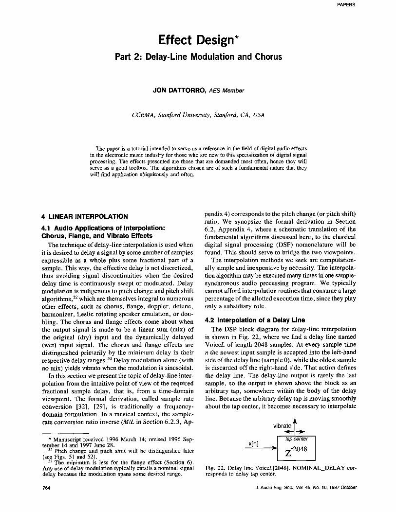
4.2 Interpolation of a Delay Line The DSP block diagram for delay-line interpolation
is shown in Fig. 22, where we find a delay line named VoiceL of length 2048 samples. At every sample time n the newest input sample is accepted into the left-hand side of the delay line (sample 0), while the oldest sample is discarded off the right-hand side. That action defines the delay line. The delay-line output is rarely the last sample, so the output is shown above the block as an arbitrary tap, somewhere within the body of the delay line. Because the arbitrary delay tap is moving smoothly about the tap center, it becomes necessary to interpolate
vibra~_T_ ~ I tap center
x[n] ~ I
-I Fig. 22. Delay line VoiceL[2048]. NOMINALDELAY cor- responds to delay tap center.
J. Audio Eng Sot., Vol 45, No. 10, 1997 October
PAPERS EFFECT DESIGN
in real t ime in between the discrete samples of the delay line. The audible effect of the tap movemen t is vibrato.
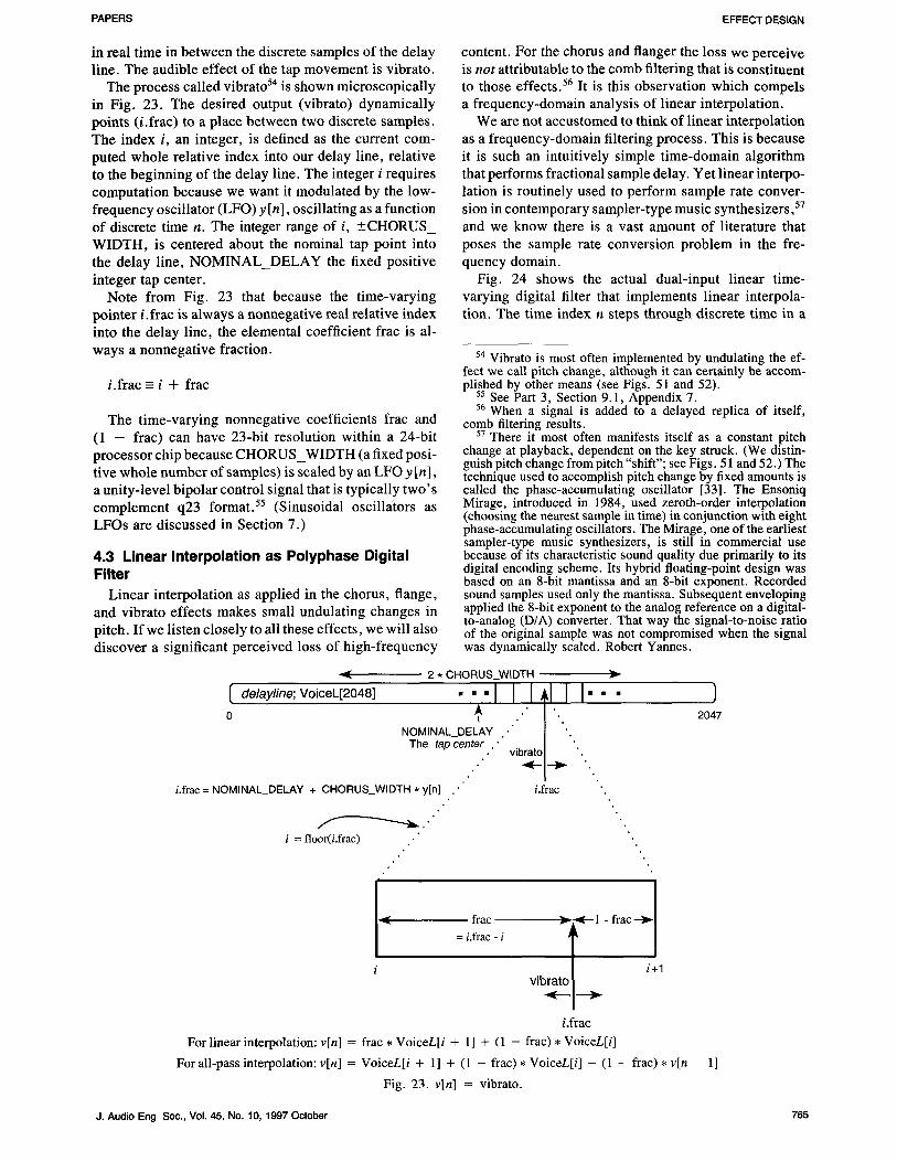
The process called vibrato 54 is shown microscopical ly in Fig. 23. The desired output (vibrato) dynamica l ly points ( i .frac) to a place between two discrete samples . The index i, an integer, is defined as the current com- puted whole relative index into our delay line, relative to the beginning of the delay line. The integer i requires computa t ion because we want it modulated by the low- f requency oscil lator (LFO) y In], oscillating as a function of discrete time n. The integer range of i, ---CHORUS_ W I D T H , is centered about the nominal tap point into the delay line, N O M I N A L D E L A Y the fixed posi t ive integer tap center.
Note f rom Fig. 23 that because the t ime-vary ing pointer i . frac is a lways a nonnegat ive real relat ive index into the delay line, the elemental coefficient frac is al- ways a nonnegat ive fraction.
i . frac = i + frac
The t ime-vary ing nonnegat ive coefficients frac and (1 - frac) can have 23-bit resolution within a 24-bit processor chip because C H O R U S _ W I D T H (a fixed posi- t ive whole number of samples) is scaled by an LFO y In], a unity-level bipolar control signal that is typical ly t w o ' s complement q23 format . 55 (Sinusoidal oscil lators as LFOs are discussed in Section 7.)
4.3 Linear Interpolation as Polyphase Digital Filter
Linear interpolation as applied in the chorus, flange, and vibrato effects makes small undulating changes in pitch. I f we listen closely to all these effects, we will also d iscover a significant perceived loss of h igh-f requency
I delaylino; VoiceL[2048]
0
content. For the chorus and flanger the loss we perceive is not attributable to the comb filtering that is constituent to those effects. 56 It is this observat ion which compels a f requency-domain analysis of linear interpolation.
We are not accustomed to think of l inear interpolation as a f requency-domain filtering process. This is because it is such an intuitively simple t ime-domain algori thm that performs fractional sample delay. Yet l inear interpo- lation is routinely used to perform sample rate conver- sion in contemporary sampler- type music synthesizers,57 and we know there is a vast amount of literature that poses the sample rate conversion p rob lem in the fre- quency domain.
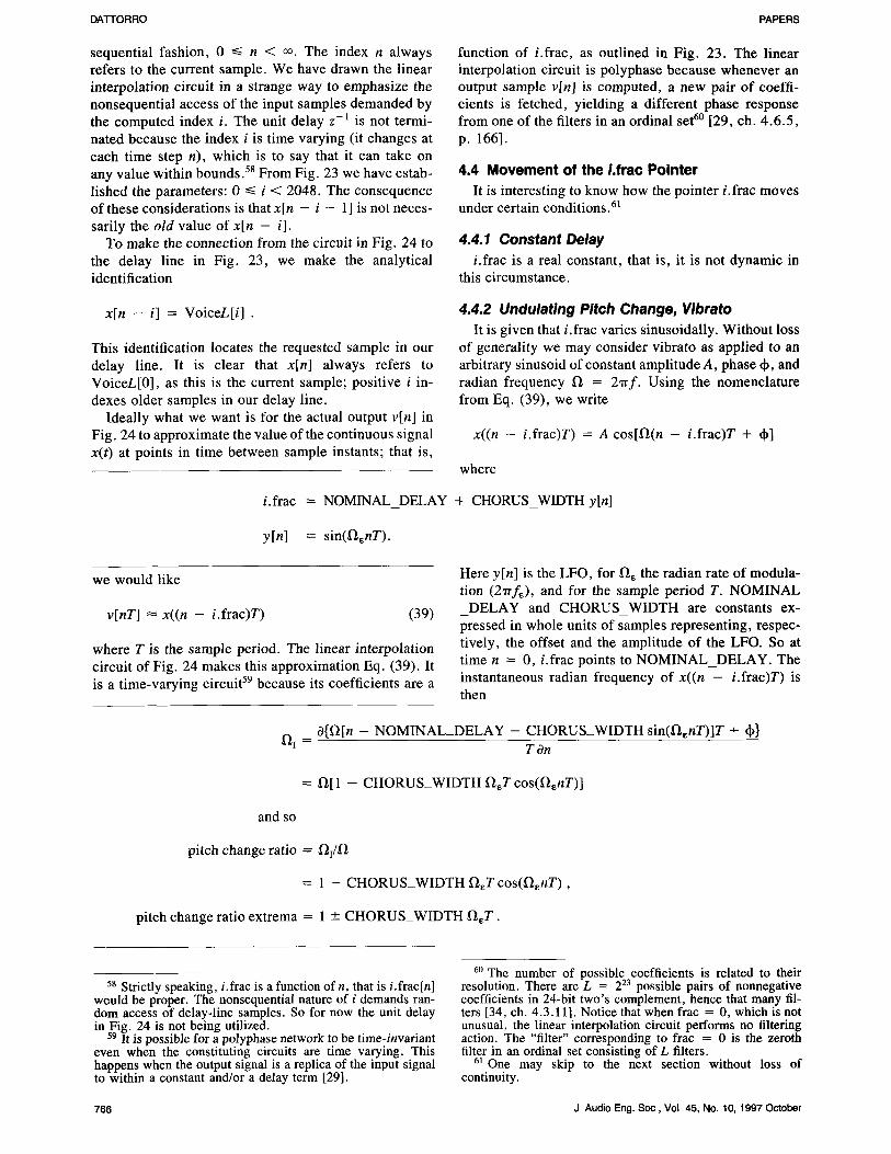
Fig. 24 shows the actual dual- input linear t ime- varying digital filter that implements l inear interpola- tion. The t ime index n steps through discrete t ime in a
54 Vibrato is most often implemented by undulating the ef- fect we call pitch change, although it can certainly be accom- plished by other means (see Figs. 51 and 52).
55 See Part 3, Section 9.1, Appendix 7. 56 When a signal is added to a delayed replica of itself,
comb filtering results. 57 There it most often manifests itself as a constant pitch
change at playback, dependent on the key struck. (We distin- guish pitch change from pitch "shift"; see Figs. 51 and 52.) The technique used to accomplish pitch change by fixed amounts is called the phase-accumulating oscillator [33]. The Ensoniq Mirage, introduced in 1984, used zeroth-order interpolation (choosing the nearest sample in time) in conjunction with eight phase-accumulating oscillators. The Mirage, one of the earliest sampler-type music synthesizers, is still in commercial use because of its characteristic sound quality due primarily to its digital encoding scheme. Its hybrid floating-point design was based on an 8-bit mantissa and an 8-bit exponent. Recorded sound samples used only the mantissa. Subsequent enveloping applied the 8-bit exponent to the analog reference on a digital- to-analog (D/A) converter. That way the signal-to-noise ratio of the original sample was not compromised when the signal was dynamically scaled. Robert Yannes.
2 * CHORUS_WIDTH ~--
NOMINAL
The tapcen ." vibrato[
." ' ~ ' - [ ' -~"
i . f r a c i.frac = NOMINAL_DELAY + CHORUS_WIDTH * y[n] �9
i = floor(i.frac)
-~ frac -~:~--- 1 - ffac I I ,
= i . f r a c - i
i + 1
vibr
i.frac For linear interpolation: v[n] = frac * VoiceL[i + 1] + (1 - frac) �9 VoiceL[i]
) 2047
For all-pass interpolation: v[n] = VoiceL[i + 1] + (1 - frac) �9 VoiceL[i] - (1 - frac) �9 v[n - 1]
Fig. 23. v[n] = vibrato.
J. Audio Eng Soc., Vol. 45, No. 10, 1997 October 765
DA'I-I'O R RO PAPERS
sequential fashion, 0 <~ n < oo. The index n always refers to the current sample. We have drawn the linear interpolation circuit in a strange way to emphasize the nonsequential access o f the input samples demanded by the computed index i. The unit delay z-~ is not termi- nated because the index i is time varying (it changes at each time step n), which is to say that it can take on any value within bounds. 58 From Fig. 23 we have estab- lished the parameters: 0 ~< i < 2048. The consequence o f these considerations is that x[n - i - 1] is not neces- sarily the old value of x[n - i].
To make the connection from the circuit in Fig. 24 to the delay line in Fig. 23, we make the analytical identification
function of i .frac, as outlined in Fig. 23. The linear interpolation circuit is polyphase because whenever an output sample v[n] is computed, a new pair o f coeffi- cients is fetched, yielding a different phase response from one of the filters in an ordinal set 6~ [29, ch. 4 .6 .5 , p. 166].
4.4 M o v e m e n t of the i . frac P o i n t e r
It is interesting to know how the pointer i .frac moves under certain conditions. 61
4.4.1 Constant Delay i.frac is a real constant, that is, it is not dynamic in
this circumstance.
x[n - i] = VoiceL[i] .
This identification locates the requested sample in our delay line. It is clear that x[n] always refers to VoiceL[0] , as this is the current sample; positive i in- dexes older samples in our delay line.
Ideally what we want is for the actual output v[n] in Fig. 24 to approximate the value of the continuous signal x(t) at points in time between sample instants; that is,
4.4.2 U n d u l a t i n g P i t c h Change, Vibrato It is given that i.frac varies sinusoidally. Without loss
o f generality we may consider vibrato as applied to an arbitrary sinusoid of constant amplitude A, phase dp, and radian frequency 12 = 2rrf . Using the nomenclature from Eq. (39), we write
x( (n - i.frac)T) = A cos[12(n - Lfrac)T + ~b]
where
i.frac = NOMINAL_DELAY + C H O R U S W I D T H y[n]
y[n] = sin(12EnT).
we would like
v[nT] ~ x ( (n - i .frac)T) (39)
where T is the sample period. The linear interpolation circuit of Fig. 24 makes this approximation Eq. (39). It is a t ime-varying circuit 59 because its coefficients are a
Here y[n] is the LFO, for I~ E the radian rate of modula- tion (27rf~), and for the sample period T. N O M I N A L
D E L A Y and CHORUS W I D T H are constants ex- pressed in whole units of samples representing, respec- tively, the offset and the amplitude of the LFO. So at time n = 0, i.frac points to N O M I N A L D E L A Y . The instantaneous radian frequency of x ( (n - i .frac)T) is then
O{~[n - N O M I N A L _ D E L A Y - C H O R U S _ W I D T H sin(12~nT)]T + ~b}
121 = T On
= 1211 - C H O R U S _ W I D T H ~ETcos(12EnT)]
and so
pitch change ratio = 1 2 t / ~
= 1 - C H O R U S _ W I D T H 12~T cos(12~nT) ,
pitch change ratio extrema = 1 - C H O R U S _ W I D T H 12~T.
58 Strictly speaking, i.frac is a function of n, that is i.frac[n] would be proper. The nonsequential nature of i demands ran- dom access of delay-line samples. So for now the unit delay in Fig. 24 is not being utilized.
s9 It is possible for a polyphase network to be time-invariant even when the constituting circuits are time varying. This happens when the output signal is a replica of the input signal to within a constant and/or a delay term [29].
60 The number of possible coefficients is related to their resolution. There are L = 223 possible pairs of nonnegative coefficients in 24-bit two's complement, hence that many fil- ters [34, ch. 4.3.11]. Notice that when frac = 0, which is not unusual, the linear interpolation circuit performs no filtering action. The "filter" corresponding to frac = 0 is the zeroth filter in an ordinal set consisting of L filters.
61 One may skip to the next section without loss of continuity.
766 J Audio Eng. Soc, Vol 45, No. 10, 1997 October
PAPERS EFFECT DESIGN
The pitch change ratio is the ratio of the new pitch 13 I to the original pitch I~. 62 In the present case, the pitch change is time varying, sinusoidal like the LFO, and proportional to the modulat ion frequency and the sample period. Note that if the LFO waveform were triangular, then the instantaneous frequency would be piecewise constant, which is unnatural.
Solving for i. frac in terms of the pitch change ratio, we determine that, in general
i .frac = n - f pitch change ratio an
where - N O M I N A L D E L A Y becomes the constant o f integration.
4.4.3 Constant Pitch Change It is given that i .frac varies linearly, that is, constant
pitch change does not imply constant delay nor constant i.frac pointer.
As before, we consider an arbitrary sinusoid of con- stant amplitude, phase, and frequency. So using Eq. (39), we again write
x ( ( n - i.frac)T) = A cos [~(n - i .frac)T + ~b]
but where
eventually pass one or the other delay-line boundary, so this technique cannot be used indefinitely.
4.5 High-Frequency Loss of Linear Interpolator We need to delve further into the connection between
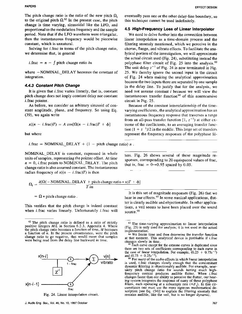
linear interpolation as a t ime-domain process and the filtering anomaly mentioned, which we perceive in the chorus, flange, and vibrato effects. To facilitate the ana- lytical portion of the investigation, we will approximate the actual circuit used (Fig. 24), substituting instead the polyphase filter circuit of Fig. 25 into the analysis. 63 The unit delay z - 1 of Fig. 24 is now terminated in Fig. 25. We thereby ignore the second input in the circuit of Fig. 24 when making the analytical approximation because the two inputs there are separated by one sample in the delay line. To justify that for the analysis, we need not assume constant i because we will view the instantaneous transfer function 64 of this nonrecursive circuit in Fig. 25.
Because of the constant interrelationship o f the time- varying coefficients, the analytical approximation has an instantaneous frequency response that traverses a range from an all-pass transfer function [1, z - ] ) at either ex- treme of the coefficients, to an averaging transfer func- tion (1 + z-1)/2 in the middle. This large set of transfers represent the frequency responses of the polyphase ill-
i .frac = N O M I N A L _ D E L A Y + (1 - pitch change r a t i o ) n .
N O M I N A L D E L A Y is constant, expressed in whole units o f samples, representing the pointer offset. At time n = 0, i .frac points to N O M I N A L DELAY. The pitch change ratio is also assumed constant. The instantaneous radian frequency of x ( ( n - i.frac)T) is then
ters. Fig. 26 shows several of these magnitude re- sponses, corresponding to 20 equispaced values of frac, that is, frac = 0-+0.95 spaced by 0.05.
= 13 �9 pitch change ra t io .
This verifies that the pitch change is indeed constant when i.frac varies linearly. Unfortunately i.frac will
a[l~(-- N O M I N A L DELAY + pitch change ratio * n ) T + ~b]
T On
It is this set of magnitude responses (Fig. 26) that we hear in our effects. 65 In some musical applications, flut- ter is clearly audible and objectionable. In other applica- tions, a veil seems to have been placed over the sound source. 66
62 The pitch change ratio is defined as a ratio of strictly positive integers M / L in Section 6.2.3, Appendix 4. Where the pitch change ratio becomes a function of time, M becomes a function of n. In the present circumstance, were the pitch change ratio to go negative, that would mean that samples were being read from the delay line backward in time.
x[n- i -1] frac
Fig. 24. Linear interpolation circuit.
v[n]
vibrato
63 The time-varying approximation to linear interpolation (Fig. 25) is only used for analysis; it is not used in the actual implementation.
64 We freeze time and then determine the transfer function at that moment. This analytical device is justifiable if i.frac changes slowly in time.
65 Each curve except for the extreme curves is duplicated since there are two sets of coefficients corresponding to each curve in the case of linear interpolation. For example, (0.25 + 0.75z -1) and (0.75 + 0.25z-1).
66 For many of the audio effects in which linear interpolation is used, i.frac changes slowly enough that the concomitant dynamic filtering is objectionably audible. For example, near- unity pitch change ratio for sounds having much high- frequency content produces audible flutter. When i.frac changes faster than our ability to perceive the flutter, our hear- ing system integrates the response of many of these polyphase filters, each operating at a subsample rate (~<Fs). In this cir- cumstance one must use the more rigorous mathematical de- scription [see Eq. (54)] to explain the filtering anomaly that remains audible, like the veil, but is no longer dynamic.
J. Audio Eng Soc., Vol. 45, No. 10, 1997 October 767
DA'R'ORRO PAPERS
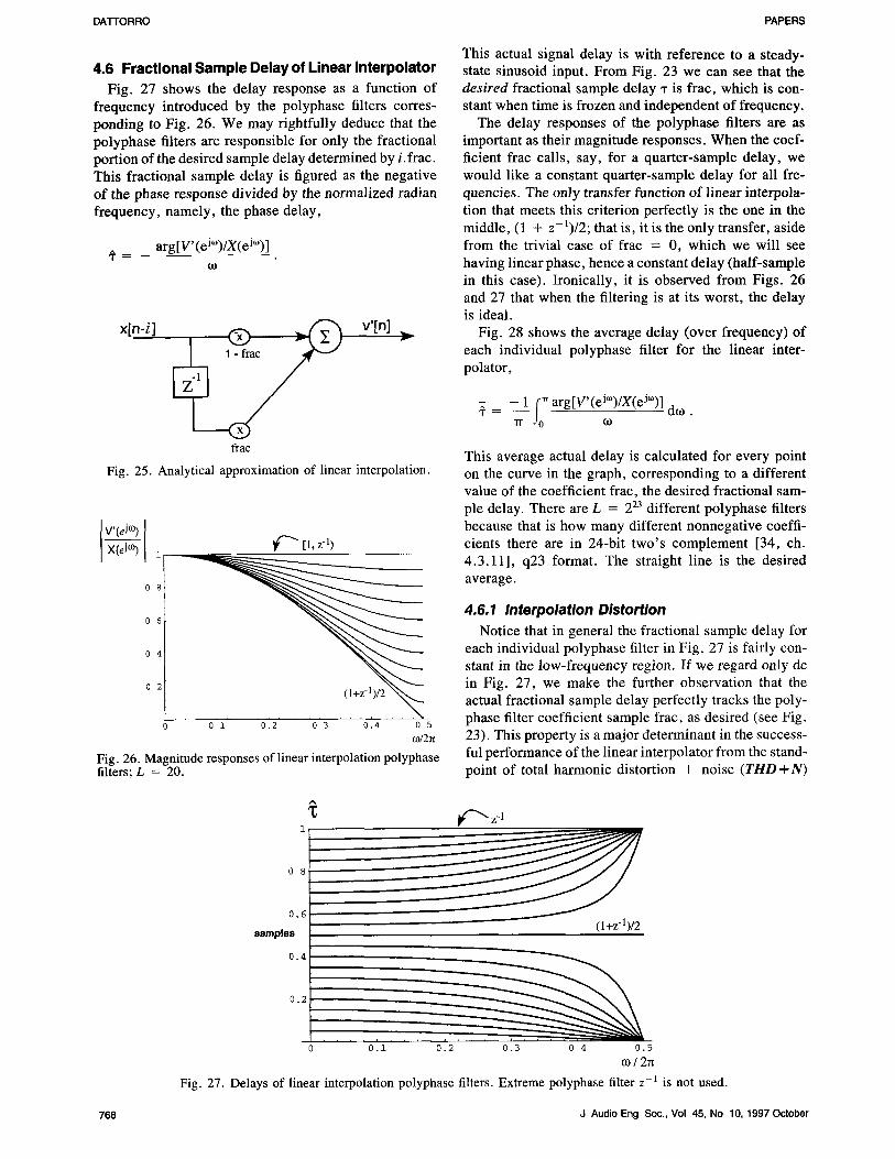
4.6 Fractional Sample Delay of Linear Interpolator Fig. 27 shows the delay response as a function of
frequency introduced by the polyphase filters corres- ponding to Fig. 26. We may rightfully deduce that the polyphase filters are responsible for only the fractional portion of the desired sample delay determined by i. frac. This fractional sample delay is figured as the negative of the phase response divided by the normalized radian frequency, namely, the phase delay,
= - arg[V'(eJ~)/X(eJ~)] 05
frar
v'[n] . . _
Fig. 25. Analytical approximation of linear interpolation.
V'(eJ c~ 1 ~ [1, Z -1)
o ,
0 6
0 4
0 2
0 1 0.2 0 3 0.4 0 5
o)/2~
Fig. 26. Magnitude responses of linear interpolation polyphase filters; L = 20.
This actual signal delay is with reference to a steady- state sinusoid input. From Fig. 23 we can see that the desired fractional sample delay "r is frac, which is con- stant when time is frozen and independent of frequency.
The delay responses of the polyphase filters are as important as their magnitude responses. When the coef- ficient frac calls, say, for a quarter-sample delay, we would like a constant quarter-sample delay for all fre- quencies. The only transfer function of linear interpola- tion that meets this criterion perfectly is the one in the middle, (1 + z - 1 ) / 2 ; that is, it is the only transfer, aside from the trivial case of frac = 0, which we will see having linear phase, hence a constant delay (half-sample in this case). Ironically, it is observed from Figs. 26 and 27 that when the filtering is at its worst, the delay is ideal.
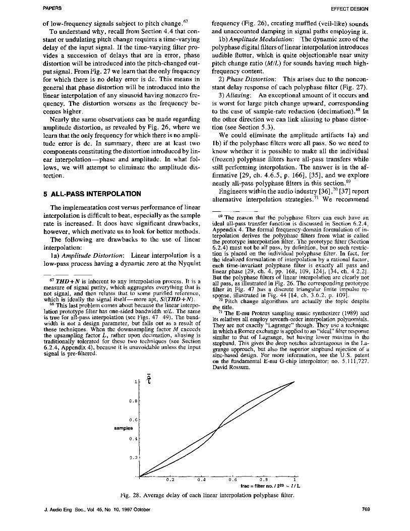
Fig. 28 shows the average delay (over frequency) of each individual polyphase filter for the linear inter- polator,
- 1 f : arg[V'(eJ~)/X(eJ=)] d o . ~ = - "rr (1)
This average actual delay is calculated for every point on the curve in the graph, corresponding to a different value of the coefficient frac, the desired fractional sam- ple delay. There are L = 223 different polyphase filters because that is how many different nonnegative coeffi- cients there are in 24-bit two's complement [34, ch. 4.3.11], q23 format. The straight line is the desired average.
4 .6 .1 I n t e r p o l a t i o n D i s t o r t i o n
Notice that in general the fractional sample delay for each individual polyphase filter in Fig. 27 is fairly con- stant in the low-frequency region. If we regard only dc in Fig. 27, we make the further observation that the actual fractional sample delay perfectly tracks the poly- phase filter coefficient sample frac, as desired (see Fig. 23). This property is a major determinant in the success- ful performance of the linear interpolator from the stand- point of total harmonic distortion + noise (THD + N )
% 1
0 8
0 , 6
samples
0.4
0 .2
ir z.l
(1+z-1)/2
i . . . . .
0 0.i 0.2 0.3 0 4 0.5
~o/2~
Fig. 27. Delays of linear interpolation polyphase filters. Extreme polyphase filter z-1 is not used.
768 J Audio Eng Soc., Vol 45, No 10, 1997 October
PAPERS EFFECT DESIGN
of low-frequency signals subject to pitch change. 67 To understand why, recall from Section 4.4 that con-
stant or undulating pitch change requires a time-varying delay of the input signal. I f the time-varying filter pro- vides a succession of delays that are in error, phase distortion will be introduced into the pitch-changed out- put signal. From Fig. 27 we learn that the only frequency for which there is no delay error is dc. This means in general that phase distortion will be introduced into the linear interpolation of any sinusoid having nonzero fre- quency. The distortion worsens as the frequency be- comes higher.
Nearly the same observations can be made regarding amplitude distortion, as revealed by Fig. 26, where we learn that the only frequency for which there is no ampli- tude error is dc. In summary, there are at least two components constituting the distortion introduced by lin- ear in terpolat ion--phase and amplitude. In what fol- lows, we will attempt to eliminate the amplitude dis- tortion.
5 A L L - P A S S I N T E R P O L A T I O N
The implementation cost versus performance of linear interpolation is difficult to beat, especially as the sample rate is increased. It does have significant drawbacks, however, which motivate us to look for better methods.
The following are drawbacks to the use of linear interpolation:
la) Amplitude Distortion: Linear interpolation is a low-pass process having a dynamic zero at the Nyquist
67 TItD +N is inherent to any interpolation process. It is a measure of signal purity~ which aggregates everything that is not signal, and then relates that to some purified reference, which is ideally the signal itself--more apt, S/(THD +N).
68 This last problem comes about because the linear interpo- lation prototype filter has one-sided bandwidth 7r/L. The same is true for all-pass interpolation (see Figs. 47-49). The band- width is not a design parameter, but falls out as a result of these techniques. When the downsampling factor M exceeds the upsampling factor L, rather upon decimation, aliasing is traditionally tolerated for these two techniques (see Section 6.2.4, Appendix 4), because it is unavoidable unless the input signal is pre-filtered.
frequency (Fig. 26), creating muffled (veil-like) sounds and unaccounted damping in signal paths employing it.
lb) Amplitude Modulation: The dynamic zero of the polyphase digital filters of linear interpolation introduces audible flutter, which is quite objectionable near unity pitch change ratio (M/L) for sounds having much high- frequency content.
2) Phase Distortion: This arises due to the noncon- stant delay response of each polyphase filter (Fig. 27).
3) Aliasing: An exceptional amount of it occurs and is worst for large pitch change upward, corresponding to the case of sample-rate reduction (decimation). 68 In the other direction we can link aliasing to phase distor- tion (see Section 5.3).
We could eliminate the amplitude artifacts la) and lb) if the polyphase filters were all pass. So we need to know whether it is possible to make all the individual (frozen) polyphase filters have all-pass transfers while still performing interpolation. The answer is in the af- firmative [29, ch. 4.6.5, p. 166], [35], and we explore nearly all-pass polyphase filters in this section. 69
Engineers within the audio industry [36] ,70 [37] report alternative interpolation strategies. 71 We recommend
0.6
samples
0.4
69 The reason that the polyphase filters can each have an ideal all-pass transfer function is discussed in Section 6.2.4, Appendix 4. The formal frequency-domain formulation of in- terpolation derives the polyphase filters from what is called the prototype interpolation filter. The prototype filter (Section 6.2.4) must not be all pass, by definition, but no such restric- tion is placed on the individual polyphase filter. In fact, for the idealized formulation of interpolation by a rational factor, each time-invariant polyphase filter is exactly all pass and linear phase [29, ch. 4, pp. 168, 109, 124], [34, ch. 4 2.2]. But the polyphase filters of linear interpolation are clearly not all pass, as illustrated in Fig. 26. The corresponding prototype filter in Fig. 47 has a discrete triangular finite impulse re- sponse, illustrated in Fig. 44 [14, ch. 3.6.2, p. 109].
70 Pitch change algorithms are actually the topic despite the title.
71 The E-mu Proteus sampling music synthesizer (1989) and its relatives all employ seventh-order interpolation polynomials. They are not exactly "Lagrange" though. They use a technique in which a Remez exchange is applied to an "ideal" filter response similar to that of Lagrange, but having lower maxima in the stopband. This gives the deep notches advantageous in the La- grange approach, but also the superior stopband rejection of a sinc-based design. For more information, see the U.S. patent on the fundamental E-mu G-chip interpolator; no. 5,111,727. David Rossum.
1 I ;
0.8
0.2
0.2 0 .4 0 . 6 0 .8 1
frac = filter no. / 223 -= I I L
Fig. 28. Average delay of each linear interpolation polyphase filter.
J. Audio Eng Soc., Vol 45, No 10, 1997 October 769
DATTORRO PAPERS
Lagrange interpolation when higher order finite impulse response (FIR) filters are a viable option [32], [34], [38], [39]. Lagrange interpolation is an analytical extension to linear interpolation. 72 But nonrecursive techniques such as these have high computational cost. Nonethe- less, FIR filters dominate contemporary sample-rate con- version practice because from the point of view of inter- nal truncation noise, it is difficult to mess up an FIR implementation [40]-[42] . Also, FIR filters offer lin- ear phase. 73
Recursive polyphase filters have not been popular be- cause they are not linear phase, in general .74 The practice of recursive digital filtering requires an understanding of fixed-point arithmetic, truncation error recirculation [12], and transient phenomena.
5.1 All-Pass Interpolation as Polyphase Digital Filter
We present here the simple recursive technique of all- pass interpolation, which is useful primarily for micro- tonal changes in pitch (less than plus or minus one semi- tone). Linear interpolation will outperform it from the standpoint of T H D + N (Section 5.4). Otherwise all-pass interpolation minimizes the drawbacks of linear interpo- lation in this microtonal region and makes the interpola- tion sound analog.
Fig. 29, a modification of Fig. 24, shows the actual circuit used to implement all-pass interpolation [43]. Our application of Fig. 29 uses time-varying filter coef- ficients. The formal derivation of the classical polyphase all-pass interpolation network [29], [35] requires as
72 That is, a higher order polynomial curve fit using more signal values, and which is maximally fiat in the frequency domain while suppressing ripple in the time domain. The two- point Lagrange interpolator is equivalent to linear interpolation.
73 Generally speaking, a linear-phase prototype interpola- tion filter does not guarantee linear-phase polyphase filters, and vice versa. Linear interpolation, for example, is an emi- nent case of an FIR prototype that is linear phase (having a symmetrical triangular impulse response of length 2L spanning two original samples by design [14, ch. 3.6.2, p. 109], [34]) but whose polyphase filters are not. Yet if a linear-phase proto- type is ideally band-limited to ~r/L, for L a rate conversion factor, then all its L polyphase filters will remain exactly linear phase [37, p. 545], [29, ch. 4.6.5, p. 168], [14, ch. 5.7]. (See Section 6.2, Appendix 4.) Crochiere and Rabiner [34, ch. 4.3.6-4.3.10] give explicit general design procedures for simultaneously linear-phase FIR polyphase and prototype in- terpolation filters.
74 Renfors and Saram~iki's infinite impulse response (IIR) design offers nearly linear-phase recursive polyphase and pro- totype interpolation filters [35].
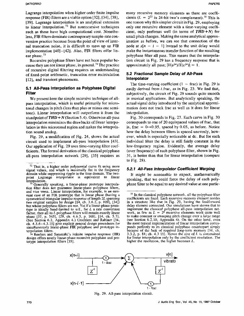
many recursive memory elements as there are coeffi- cients (L = 223 in 24-bit two's complement). 7s This is one reason why this simpler circuit in Fig. 29, employing only one recursive element with a time-varying coeffi- cient, only performs well (in terms of T H D + N ) for small pitch changes. Making the same analytical approx- imation as before, we can see that connection of the node at x[n - i - 1] instead to the unit delay would make the instantaneous transfer function of the resulting polyphase filter all pass. This means that the interpola- tion circuit in Fig. 29 has a frequency response that is approximately all pass; IV(eJ~o)/X(eJ~)l ~ 1.
5.2 Fractional Sample Delay of All-Pass Interpolator
The time-varying coefficient (1 - frac) in Fig. 29 is easily derived from i.frac, as in Fig. 23. We find that, subjectively, the circuit of Fig. 29 sounds quite smooth in musical applications. But analytically speaking, the actual signal delay introduced by the analytical approxi- mation does not track frac as well as it does for linear interpolation.
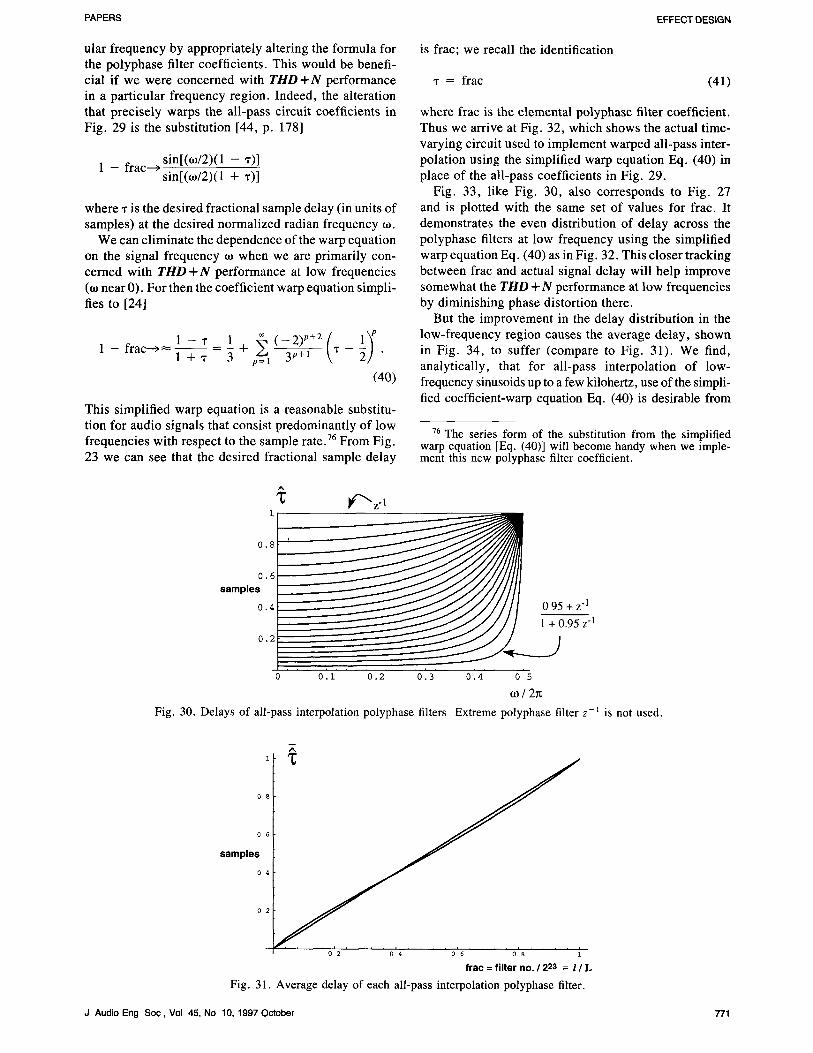
Fig. 30 corresponds to Fig. 27. Each curve in Fig. 30 corresponds to one of 20 equispaced values of frac, that is, frac = 0---*0.95, spaced by 0.05, as before. Notice how the delay between filters is spaced unevenly, how- ever, which is especially noticeable at de. But for each individual filter the delay is still fairly constant in the low-frequency region. Evidently, the average delay (over frequency) of each polyphase filter, shown in Fig. 31, is better than that for linear interpolation (compare to Fig. 28).
5.2.1 All-Pass Interpolator Coefficient Warping It might be reasonable to expect, mathematically
speaking, that we could force the delay of each poly- phase filter to be equal to any desired value at one partic-
75 In the classical polyphase network, all the polyphase filter coefficients are fixed. Each recursive memory element resides in a structure like that in Fig. 29, having the feedforward delay element connected. Our simulations have shown that to implement the classical polyphase all-pass interpolation net- work, as few as L = 28 recursive elements work quite well to make constant or sweeping pitch change over a large range (see Section 6.2.10, Appendix 4). On the other hand, even the most typical implementation of linear interpolation corres- ponds perfectly to its classical polyphase counterpart simply because of the lack of required long-term memory [34, ch. 3.3.2, p. 81; ch. 4.3 I1]. Hence the size of L is constrained for linear interpolation only by the coefficient resolution. The higher the resolution, the higher becomes L.
x [ n - i ]
x [ n - i - 1 ]
v[n]
~ ibrato
1 - frac
Fig. 29. All-pass interpolation circuit.
770 J Audio Eng Soc, Vol 45, No 10, 1997 October
PAPERS EFFECT DESIGN
ular frequency by appropriately altering the formula for the polyphase filter coefficients. This would be benefi- cial if we were concerned with T H D + N performance in a particular frequency region. Indeed, the alteration that precisely warps the all-pass circuit coefficients in Fig. 29 is the substitution [44, p. 178]
1 - frac.__,sinL,to/2,,lr( ~( T)]
sin[((o/2)(1 + "r)]
where ,r is the desired fractional sample delay (in units of samples) at the desired normalized radian frequency (o.
We can eliminate the dependence of the warp equation on the signal frequency (o when we are primarily con- cerned with T I t D + N performance at low frequencies ((~ near 0). For then the coefficient warp equation simpli- fies to [24]
1 - frac---~ 1 - - ' r 1
l + ' r 3 p = l 3 p + I T -- .
(40)
This simplified warp equation is a reasonable substitu- tion for audio signals that consist predominantly of low frequencies with respect to the sample rate. 76 From Fig. 23 we can see that the desired fractional sample delay
is frac; we recall the identification
"r = frac (41)
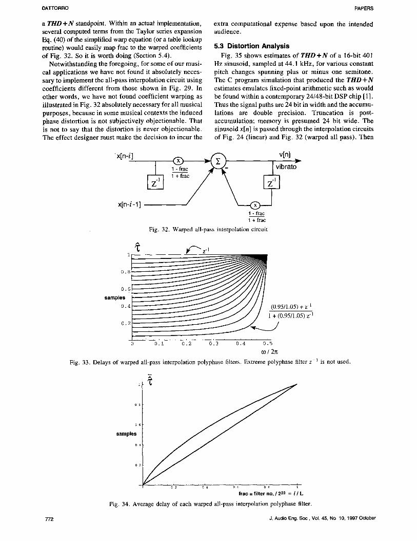
where frac is the elemental polyphase filter coefficient. Thus we arrive at Fig. 32, which shows the actual time- varying circuit used to implement warped all-pass inter- polation using the simplified warp equation Eq. (40) in place of the all-pass coefficients in Fig. 29.
Fig. 33, like Fig. 30, also corresponds to Fig. 27 and is plotted with the same set of values for frac. It demonstrates the even distribution of delay across the polyphase filters at low frequency using the simplified warp equation Eq. (40) as in Fig. 32. This closer tracking between frac and actual signal delay will help improve somewhat the T H D -t- N performance at low frequencies by diminishing phase distortion there.
But the improvement in the delay distribution in the low-frequency region causes the average delay, shown in Fig. 34, to suffer (compare to Fig. 31). We find, analytically, that for all-pass interpolation of low- frequency sinusoids up to a few kilohertz, use of the simpli- fied coefficient-warp equation Eq. (40) is desirable from
76 The series form of the substitution from the simplified warp equation [Eq. (40)] will become handy when we imple- ment this new polyphase filter coefficient.
~ , , , , z.1 1
0 . 6 samples
~ I
95 z -1 0 . 2
0 ' 0'.i 0.2 0.3 0.4 0 5
c0/2n
Fig. 30. Delays of all-pass interpolation polyphase filters Extreme polyphase filter z-' is not used.
samples
m A
1 I ;
o B
o 6
s
o 4
o 2
, , , , 012 ' , , , 014 ' , , , 016 ' , , , = , , , , = 0 8 1
frac = filter no. / 223 ~- l / [,
Fig. 31. Average delay of each all-pass interpolation polyphase filter.
J Audio Eng Soc, Vol 45, No 10, 1997 October 771
DATrORRO PAPERS
a THD + N standpoint. Within an actual implementation, several computed terms from the Taylor series expansion Eq. (40) of the simplified warp equation (or a table lookup routine) would easily map frac to the warped coefficients of Fig. 32. So it is worth doing (Section 5.4).
Notwithstanding the foregoing, for some of our musi- cal applications we have not found it absolutely neces- sary to implement the all-pass interpolation circuit using coefficients different from those shown in Fig. 29. In other words, we have not found coefficient warping as illustrated in Fig. 32 absolutely necessary for all musical purposes, because in some musical contexts the induced phase distortion is not subjectively objectionable. That is not to say that the distortion is never objectionable. The effect designer must make the decision to incur the
extra computational expense based upon the intended audience.
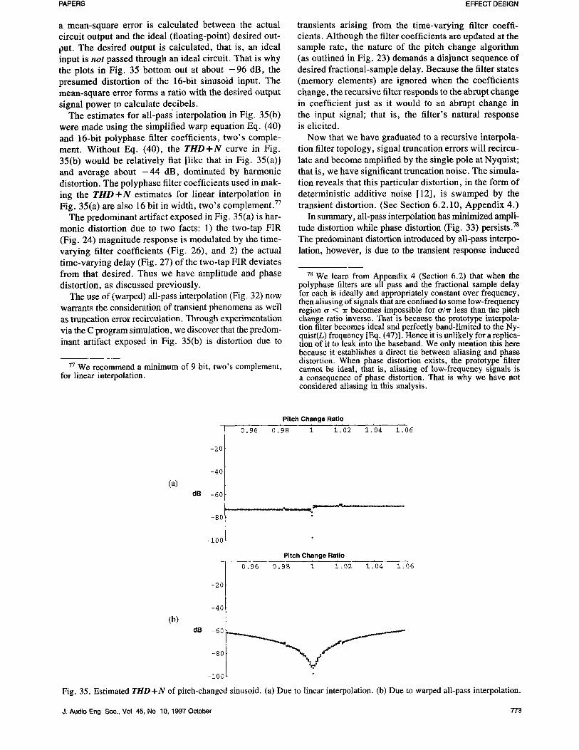
5.3 Distortion Analysis Fig. 35 shows estimates of T H D + N of a 16-bit 401
Hz sinusoid, sampled at 44.1 kHz, for various constant pitch changes spanning plus or minus one semitone. The C program simulation that produced the TItD + N estimates emulates fixed-point arithmetic such as would be found within a contemporary 24/48-bit DSP chip [1]. Thus the signal paths are 24 bit in width and the accumu- lations are double precision. Truncation is post- accumulation; memory is presumed 24 bit wide. The sinusoid x[n] is passed through the interpolation circuits of Fig. 24 (linear) and Fig. 32 (warped all pass). Then
'x[n-i]
•
~%~ v i [n] brato
Q 1 - frac
1 + frac
Fig. 32. Warped all-pass interpolation circuit
f~-zl
0 . I
0.1
samples
0 . ,
0 . :
5/1.05) + z -1
D.95/1.05) z -1
0 0.i 0.2 0.3 0.4 0.5
co/2~ Fig. 33. Delays of warped all-pass interpolation polyphase filters. Extreme polyphase filter z-1 is not used.
A
0
0
samples
0
0
. . . . i . . . . i 02 04 06 08 1
frac = filter no. / 223 -= l / L
Fig. 34. Average delay of each warped all-pass interpolation polyphase filter.
772 J. Audio Eng. Soc, Vol. 45, No 10, 1997 October
PAPERS EFFECT DESIGN
a mean-square error is calculated between the actual circuit output and the ideal (floating-point) desired out- put. The desired output is calculated, that is, an ideal input is not passed through an ideal circuit. That is why the plots in Fig. 35 bottom out at about - 9 6 dB, the presumed distortion of the 16-bit sinusoid input. The mean-square error forms a ratio with the desired output signal power to calculate decibels.
The estimates for all-pass interpolation in Fig. 35(b) were made using the simplified warp equation Eq. (40) and 16-bit polyphase filter coefficients, two's comple- ment. Without Eq. (40), the T H D + N curve in Fig. 35(b) would be relatively flat [like that in Fig. 35(a)] and average about - 4 4 dB, dominated by harmonic distortion. The polyphase filter coefficients used in mak- ing the THD + N estimates for linear interpolation in Fig. 35(a) are also 16 bit in width, two's complement. 77
The predominant artifact exposed in Fig. 35(a) is har- monic distortion due to two facts: 1) the two-tap FIR (Fig. 24) magnitude response is modulated by the time- varying filter coefficients (Fig. 26), and 2) the actual time-varying delay (Fig. 27) of the two-tap FIR deviates from that desired. Thus we have amplitude and phase distortion, as discussed previously.
The use of (warped) all-pass interpolation (Fig. 32) now warrants the consideration of transient phenomena as well as truncation error recirculation. Through experimentation via the C program simulation, we discover that the predom- inant artifact exposed in Fig. 35(b) is distortion due to
77 We recommend a minimum of 9 bit, two's complement, for linear interpolation.
transients arising from the time-varying filter coeffi- cients. Although the filter coefficients are updated at the sample rate, the nature of the pitch change algorithm (as outlined in Fig. 23) demands a disjunct sequence of desired fractional-sample delay. Because the filter states (memory elements) are ignored when the coefficients change, the recursive filter responds to the abrupt change in coefficient just as it would to an abrupt change in the input signal; that is, the filter's natural response is elicited.
Now that we have graduated to a recursive interpola- tion filter topology, signal truncation errors will recircu- late and become amplified by the single pole at Nyquist; that is, we have significant truncation noise. The simula- tion reveals that this particular distortion, in the form of deterministic additive noise [12], is swamped by the transient distortion. (See Section 6.2.10, Appendix 4.)
In summary, all-pass interpolation has minimized ampli- tude distortion while phase distortion (Fig. 33) persists. 7s The predominant distortion introduced by all-pass interpo- lation, however, is due to the transient response induced
78 We learn from Appendix 4 (Section 6.2) that when the polyphase filters are all pass and the fractional sample delay for each is ideally and appropriately constant over frequency, then aliasing of signals that are confined to some low-frequency region ~r < ~r becomes impossible for tr/~r less than the pitch change ratio inverse. That is because the prototype interpola- tion filter becomes ideal and perfectly band-limited to the Ny- quist(L) frequency [Eq. (47)]. Hence it is unlikely for a replica- tion of it to leak into the baseband. We only mention this here because it establishes a direct tie between aliasing and phase distortion. When phase distortion exists, the prototype filter cannot be ideal, that is, aliasing of low-frequency signals is a consequence of phase distortion. That is why we have not considered aliasing in this analysis.
(a)
(b)
dB
dB
-2(
-40
-60
-80
-i00
Pitch Change Ratio
0.96 0.98 1 1.02 1.04 1.06
~..-i[ i n I .
Pitch Change Ratio
0.96 0.98 1 1.02 1.04 1.06
-2
-40
- 8 0 ""~% ]/J %. ~.."
-i00
Fig. 35. Estimated TItD + N of pitch-changed sinusoid. (a) Due to linear interpolation. (b) Due to warped all-pass interpolation.
J. Audio Eng Soc., Vol 45, No 10, 1997 October 773
DA]3 OHHU PAI'q:H~
by the time-varying filter coefficients in the recursive interpolation circuit. This type of distortion is not pres- ent for the linear interpolator. It is that transient distor- tion which bottlenecks the useful transposition range of the all-pass interpolator to about plus or minus one semitone. There is a way to overcome this particular problem (which is discussed in Section 6.2.10, Appen- dix 4), but the solution adds more computational expense.
5.4 Implementations of All-Pass Interpolation Now we leave the realm of simulation and estimation
to visit the reality of actual implementation and measure- ment. Establishing the sinusoidal LFO frequency = 0.1 Hz in a real-time 24/48-bit DSP hardware develop- ment system, we put a 24-bit 400-Hz sinusoid through a delay line, perform delay modulation, then send the 16-bit vibrato output (as in Fig. 22) to an Audio Preci- sion signal analyzer. All polyphase filter coefficients are now 24 bit, the sample rate is 44.1 kHz to within 0.001% accuracy, and truncation is post-accumulation.
We require that the implementation of the interpola- tion circuit (in Fig. 29) prevent prolonged Nyquist (Fs/2) oscillation that comes about when frac = 0. We can accomplish this by forcing that circuit to interpolate by a constant fraction of a sample at all times, say, 1/256 sample. This technique introduces a constant fractional offset into the equation for i.frac in Fig. 23 (not shown there) and has little deleterious audible consequence,
5.5 Conclusions Having reached parity between the two processes in
terms of T H D + N , we would preferentially choose warped all-pass interpolation because it minimizes the drawbacks of linear interpolation, stated at the outset of this section, when used in a microtonal region. If the added computation to warp the coefficients is not af- fordable, then (nonwarped) all-pass interpolation is a viable alternative because it sounds better than linear interpolation in some musical contexts. Its computa- tional complexity is only slightly greater than that of linear interpolation, and it minimizes amplitude distortion.
In Appendix 4 (Section 6.2) we present the classical polyphase warped all-pass interpolator as a means of pitch change over a much larger range and to a higher degree of accuracy in terms of THD + N. It is primarily of theoretical interest, being computationally expensive by today's standards.
Are we on the right track? This idea of using all-pass filters to perform interpolation is somewhat foreign. But as we discover in Appendix 4, the linear-phase all-pass filter is the ideal polyphase filter in the classical formula- tion of interpolation [Eq. (39)] by a rational factor. So the answer is, yes indeed.
5.6 Theoretical Extensions Laakso et al. [39] broaden the scope of this warped
all-pass approach to interpolation. They provide formu-
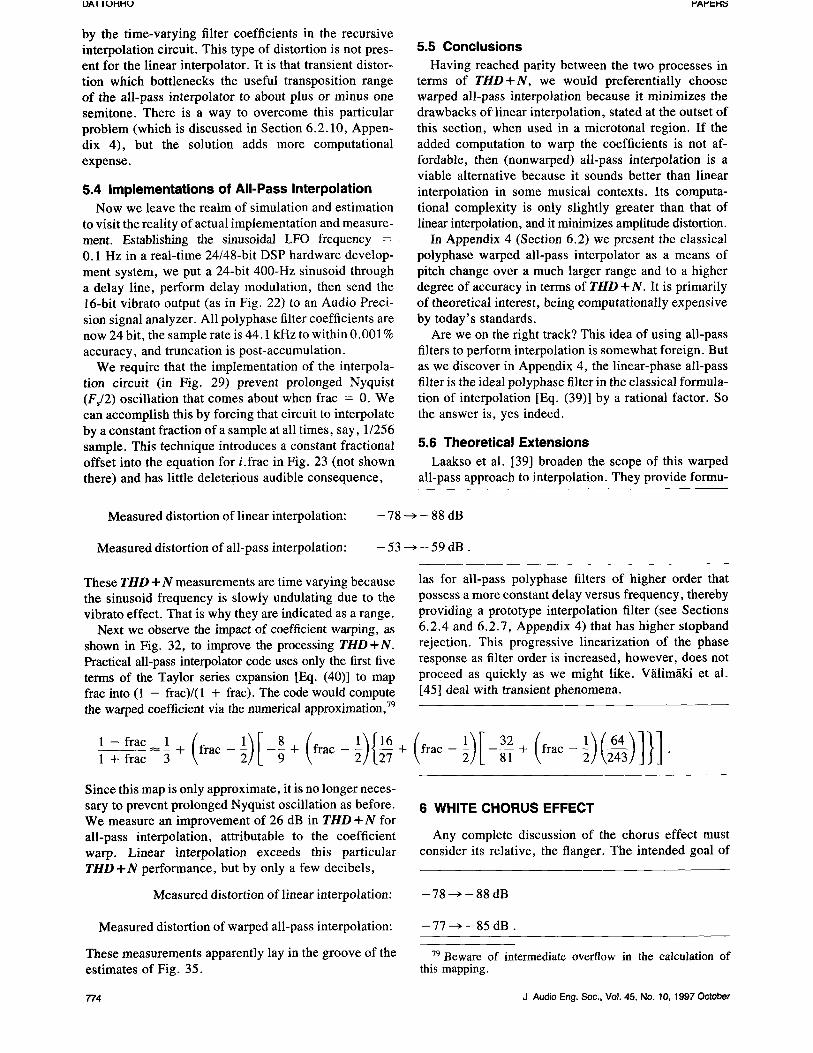
Measured distortion of linear interpolation: - 78 ~ - 88 dB
Measured distortion of all-pass interpolation: - 53 ~ - 59 dB.
These THD + N measurements are time varying because the sinusoid frequency is slowly undulating due to the vibrato effect. That is why they are indicated as a range.
Next we observe the impact of coefficient warping, as shown in Fig. 32, to improve the processing THD +N. Practical all-pass interpolator code uses only the first five terms of the Taylor series expansion [Eq. (40)] to map frac into (1 - frac)/(1 + frac). The code would compute the warped coefficient via the numerical approximation, 79
las for all-pass polyphase filters of higher order that possess a more constant delay versus frequency, thereby providing a prototype interpolation filter (see Sections 6.2.4 and 6.2.7, Appendix 4) that has higher stopband rejection. This progressive linearization of the phase response as filter order is increased, however, does not proceed as quickly as we might like. V~ilim~iki et al. [45] deal with transient phenomena.
1 - f r a c 1 ( 1 ) [ 8 ( 1]~16 1 + f r a Y = 3 + f r a c - - ~ + f r a c - 2 J L ~ + ( f r a c - 1 ) [ - ~ + ( f r a c - 1 ) ( 2 ~ 3 ) ] } ] -
Since this map is only approximate, it is no longer neces- sary to prevent prolonged Nyquist oscillation as before. We measure an improvement of 26 dB in TtID -I- N for all-pass interpolation, attributable to the coefficient warp. Linear interpolation exceeds this particular THD + N performance, but by only a few decibels,
6 WHITE CHORUS EFFECT
Any complete discussion of the chorus effect must consider its relative, the flanger. The intended goal of
Measured distortion of linear interpolation: - 78 ~ - 88 dB
Measured distortion of warped all-pass interpolation: - 77 ~ - 85 dB.
These measurements apparently lay in the groove of the estimates of Fig. 35.
79 Beware of intermediate overflow in the calculation of this mapping.
774 J Audio Eng. Soc., VoL 45, No. 10, 1997 October
PAPERS EFFECT DESIGN
chorusing is to emulate the independence of multiple like-voices playing in unison. But the goal of flanging is to jolt the ear 's time-correlation mechanism by juxta- position of the input signal with a replica dynamically delayed by an amount that is within the integration time constant of the hearing system. 8~ We must first note that there is a very strong bond between the design of the chorus effect and of the sonically radical flange effect. What has gestated into the industry standard for both members of this species condenses simply to a sum of the original input signal with a dynamically delayed replica, namely, two voices. In either effect, the replica delay is modulating and never static. So the consequence of summing the two signals is to introduce a comb of moving troughs into the input signal spectrum [46]. In the case of flanging, that is the desired result. The deeper and more selective the troughs are, the better, s~ In the case of chorusing, the troughs are undesirable and an effort is made to globally limit their depth by summing unequal amounts of original signal and delayed replica. But the primary distinguishing design feature of the chorus is that the minimum of its modulating delay time is greater than that for the flange effect. This is to avoid flanging by the chorus, which becomes subjectively more pronounced for small delays. Indeed, the best
s0 The familiar thunder of a jet aircraft often reaches our ears by combination in air of the direct and the reflected engine backwash. As the aircraft changes position, the reflection time changes, and Doppler pitch change due to the aircraft's reces- sion is introduced into both paths. The roar is more interesting as the reflection time is swept. That introduces more Doppler into the reflected path.
Sl The flange effect gets its name from a studio technique that sums two synchronous magnetic-tape-recorder signals playing identical material. The recording engineer places the thumb on one tape flange to bring the two recorders slightly out of synchronization, thus creating the effect. In the 1970s the flange effect was emulated by analog phase-shifting net- works consisting of a cascade of all-pass filters having time- varying elements. Implemented in this manner, the problem of delaying a signal by brute force was overcome. These de- vices were called phasers and remain popular because the spec- tral troughs are not harmonically spaced, in general. While second-order all-pass filter sections in the cascade offer more control over trough frequency and selectivity [46], the phaser is well emulated in DSP using only first-order sections [47], [48] (which may be quieter in terms of truncation noise per- formance). The spectral trough frequencies are harmonically stretched in the first-order case. In any case, global feedback enhances the effect, affecting the perceived trough depth.
flangers can sweep the delay all the way to absolute zero, that is, to no delay.
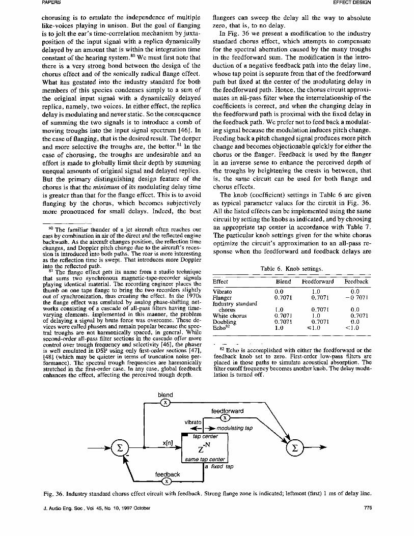
In Fig. 36 we present a modification to the industry standard chorus effect, which attempts to compensate for the spectral aberration caused by the many troughs in the feedforward sum. The modification is the intro- duction of a negative feedback path into the delay line, whose tap point is separate from that of the feedforward path but fixed at the center of the modulating delay in the feedforward path. Hence, the chorus circuit approxi- mates an all-pass filter when the interrelationship of the coefficients is correct, and when the changing delay in the feedforward path is proximal with the fixed delay in the feedback path. We prefer not to feed back a modulat- ing signal because the modulation induces pitch change. Feeding back a pitch changed signal produces more pitch change and becomes objectionable quickly for either the chorus or the flanger. Feedback is used by the flanger in an inverse sense to enhance the perceived depth of the troughs by heightening the crests in between, that is, the same circuit can be used for both flange and chorus effects.
The knob (coefficient) settings in Table 6 are given as typical parameter values for the circuit in Fig. 36. All the listed effects can be implemented using the same circuit by setting the knobs as indicated, and by choosing an appropriate tap center in accordance with Table 7. The particular knob settings given for the white chorus optimize the circuit 's approximation to an all-pass re- sponse when the feedforward and feedback delays are
Table 6. Knob settings.
Effect Blend Feedforward Feedback
Vibrato 0.0 1.0 0.0 Flanger 0.7071 0.7071 - 0 7071 Industry standard
chorus 1.0 0.7071 0.0 White chorus 0.7071 1.0 0.7071 Doubling 0.7071 0.7071 0.0 Echo s2 1.0 ~< 1.0 < 1.0
82 Echo is accomplished with either the feedforward or the feedback knob set to zero. First-order low-pass filters are placed in those paths to simulate acoustical absorption. The filter cutoff frequency becomes another knob. The delay modu- lation is turned off.
blend feedforward ~ % ~
vibrato [ - - - - - - @ I ~ modulating tap
F tap center x[n]
- - Z N
I same tap center l a fixed tap feedback
Q Fig. 36. Industry standard chorus effect circuit with feedback. Strong flange zone is indicated; leftmost (first) 1 ms of delay line.
J. Audio Eng. Soc, Vol 45, No 10, 1997 October 775
DAI-FORRO PAPERS
proximal. To maintain that optimization, the feedfor- ward coefficient must remain 1.0 while the blend and feedback coefficients remain equal,
ncho~ , ( z ) = blend + feedforward z - i
I + feedback Z-same tapc~,~, �9
Under the stated conditions on the coefficients, [Hcho,~s(eJ~)[ = I when i = same tap center. When the circuit in Fig. 36 performs flanging, the blend and feedf- orward coefficients must be equal for maximum trough depth. The maximum magnitude of feedback is 0.9999999 (q23) for stability of all the effects.
For the white chorus effect introduced here, an inter- esting delay tap center ( N O M I N A L D E L A Y ; Fig. 23) would be 400 samples at F s = 44.1 kHz, whereas a musically useful peak delay excursion ( C H O R U S WIDTH) of the modulation about the tap center would be approximately 350 samples. A typical rate of modulation would be about 0.15 Hz.
Table 7. Approximate effect delay range in milliseconds.
Effect Onset Nominal Range End
Vibrato 83 0 Minimal 5 Flange 0 1 10 Chorus 1 5 30 Doubling 10 20 100 Echo 50 80
6.1 Chorus Effect Design The circuit in Fig. 36 produces a brilliant tone quality,
having pleasing movement with a little spatial ambience. Used singly and without feedback, this circuit 's effect is called doubl ing 84 when the delay tap center reaches about 20 ms. 85
The circuit in Fig. 36 is so simple that it is economical to use two of them. Each would process a separate chan- nel of a stereo input signal. In that design configuration, a quadrature LFO typically provides the delay modulator so that each chorus circuit operates having 90 ~ relative phase displacement of its modulation .86 Each circuit out- put would be routed to a separate channel in a stereo pair. This quadrature strategy dynamically alters the stereo placement of the output signal in a pleasing way. Were the input signal monophonic, a dynamic stereo field would be created. The stereo field occurs because a time- delay difference between two output channels carrying coherent signals elicits a localization cue. This is known
83 NOMINALDELAY is usually made to track the depth of vibrato (CHORUS_WIDTH; Fig. 23) in the best vibrato algorithms, that is, the smaller the better.
84 Previously known as double tracking, a singer would at- tempt to record the same performance onto a second track while listening to the first. When machines became available to emulate this effect in real time, thereby saving a track, it became known as doubling. The delay modulation is best randomized for the doubling effect
85 Fixed at about 80 ms, we discovered that you get the Elvis Presley echo effect. George Martin.
86 Section 7 on sinusoidal oscillators discloses highly effi- cient quadrature designs.
776
as the Haas effect. While musically interesting, Haas is a persistent source of irritation for recording engineers attempting to place a musical instrument accurately into a stereo mix. For this reason it is prudent to place a stereo field control (or a panning circuit) at the output of any chorus algorithm. It is also useful to have a user switch for disabling the quadrature modulation, that is, for in-phase modulation. (Antiphase is also an option.)
I f the flange effect utilizes the same two circuits for stereo processing as did the stereo chorus, then the flanger would normally incorporate delay modulation of the same phase in each channel. Otherwise the comb filtering is diminished due to acoustic mixing in air at the loudspeaker output. The strong flange zone occupies approximately the first 1 ms of the delay line. The viable regions of delay excursion for the chorus and flange effects overlap, however, and can be determined easily by ear. Table 7 gives the approximate delay range and the nominal setting of tap center for the various effects achievable by the circuit of Fig. 36. From the range end one can determine a suitable estimate of the delay-line size N.
It is important to keep the chorus circuit free of nonlin- earity for those many guitarists who want the chorus effect as clean and clear as possible. For them, simplicity of the chorus design is a virtue as they use this effect almost all the time. Hence all-pass interpolation 87 for delay modulation becomes critical to the transparency of any chorus. Recall that linear interpolation is a time- varying low-pass filtering process. Indeed, a multivoice (more than two) chorus design using linear interpolation subjects the signal to significantly audible amounts of low-pass filtering attributable to the interpolation. We term the chorus whi te when both negative feedback and all-pass interpolation are used to minimize the spectral aberration that would occur in the absence of these two signal-processing techniques.
Flangers, on the other hand, can benefit from a mild memoryless nonlinearity introduced into the input signal path which resides in front of the entire effect, so that the flange-induced troughs see a richer signal source. But all-pass interpolation is also critical to successful flanger design so as to ensure that the dynamically de- layed signal remains unfiltered. The low-pass filtering of the delayed signal, introduced as an artifact of linear interpolation, will reduce the depth of the high- frequency troughs. This is undesirable for a good flanger.
6.2 Appendix 4: Multirate Audio Processes The purpose of this appendix is to make a rigorous
connection between the formal DSP approach to interpo- lation and decimation, and the time-domain formulation by fractional sample delay as presented in the interpola- tion sections. The reading of this material is optional and suggested only for those who are already familiar with the viewpoint of Vaidyanathan or Crochiere [29],
87 As discussed in Section 5.
J. Audio Eng. Soe, Vol. 45, No. 10, 1997 October
PAPERS EFFECT DESIGN
[34], [14, ch. 3.6] and who are comfortable with the z transform.
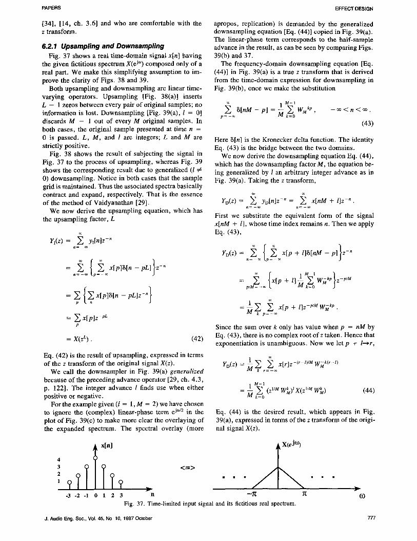
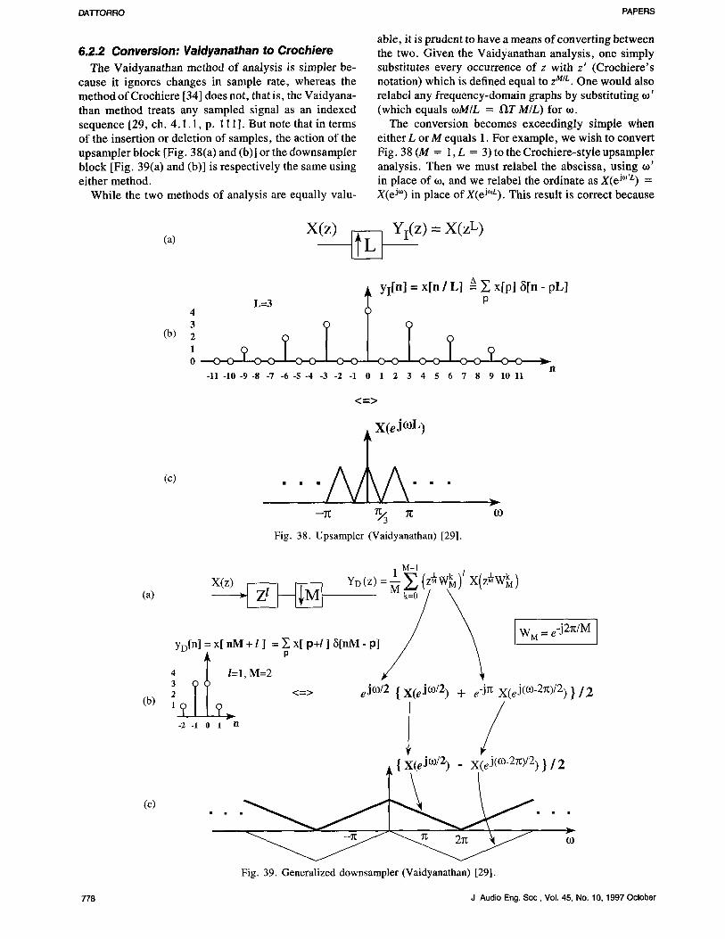
6.2.1 Upsampling and Downsampling Fig. 37 shows a real time-domain signal x[n] having
the given fictitious spectrum X(e j=) composed only of a real part. We make this simplifying assumption to im- prove the clarity of Figs. 38 and 39.
Both upsampling and downsampling are linear time- varying operators. Upsampling [Fig. 38(a)] inserts L - 1 zeros between every pair of original samples; no information is lost. Downsampling [Fig. 39(a), l = 0] discards M - 1 out of every M original samples. In both cases, the original sample presented at time n = 0 is passed. L, M, and 1 are integers; L and M are strictly positive.
Fig. 38 shows the result of subjecting the signal in Fig. 37 to the process of upsampling, whereas Fig. 39 shows the corresponding result due to generalized (l # 0) downsampling. Notice in both cases that the sample grid is maintained. Thus the associated spectra basically contract and expand, respectively. That is the essence of the method of Vaidyanathan [29].
We now derive the upsampling equation, which has the upsampling factor, L
Yi(z) = ~ yi[n]z -n n = -co
= [p]g[n - pL z-" n = - - ~ p
= ~ x[p]z -pL p
= X(zL). (42)
Eq. (42) is the result of upsampling, expressed in terms of the z transform of the original signal X(z).
We call the downsampler in Fig. 39(a) generalized because of the preceding advance operator [29, ch. 4.3, p. 122]. The integer advance l finds use when either positive or negative.
For the example given (l = 1, M = 2) we have chosen to ignore the (complex) linear-phase term e j~ in the plot of Fig. 39(c) to make more clear the overlaying of the expanded spectrum. The spectral overlay (more
apropos, replication) is demanded by the generalized downsampling equation [Eq. (44)] copied in Fig. 39(a). The linear-phase term corresponds to the half-sample advance in the result, as can be seen by comparing Figs. 39(b) and 37.
The frequency-domain downsampling equation [Eq. (44)] in Fig. 39(a) is a true z transform that is derived from the time-domain expression for downsampling in Fig. 39(b), once we make the substitution
IM-I ~[nM - p] = ~ k~=o W~t kp ,
p = - o o =
-oo<n<oo.
(43)
Here $[n] is the Kronecker delta function. The identity Eq. (43) is the bridge between the two domains.
We now derive the downsampling equation Eq. (44), which has the downsampling factor M, the equation be- ing generalized by l an arbitrary integer advance as in Fig. 39(a). Taking the z transform,
YD(Z) = ~ yD[n]z - n = ~ x[nM + l]z -n . It= -oo n= -oo
First we substitute the equivalent form of the signal x[nM + l], whose time index remains n. Then we apply Eq. (43),
YD(Z) = [p + I]a[nM - p z-" n = - - o o p
+( 1=,} : +
= __1 ~k ~oo x[p + I]z-P/M W~tkP M p=_
Since the sum over k only has value when p = n M by Eq. (43), there is no complex root of z taken. Hence that exponentiation is unambiguous. Now we let p + l--+r,
~__ L Z r ~oo X[F]Z-(r-I)/M WMk(r-l> YD(Z) M k =-
1M-1 = (z ,,M (44)
Eq. (44) is the desired result, which appears in Fig. 39(a), expressed in terms of the z transform of the origi- nal signal X(z).
?
-3 i
x[n]
TIIT < ' >
-2-1 0 1 2 3 n --~ 7~ 0.) Fig. 37. Time-limited input signal and its fictitious real spectrum.
J. Audio Eng. Soc., Vol. 45, No 10, 1997 October 777
DATTORRO PAPERS
6.2.2 Conversion: Vaidyanathan to Crochiere The Vaidyanathan method of analysis is simpler be-
cause it ignores changes in sample rate, whereas the method of Crochiere [34] does not, that is, the Vaidyana- than method treats any sampled signal as an indexed sequence [29, ch. 4.1.1, p. 111 ]. But note that in terms of the insertion or deletion of samples, the action of the upsampler block [Fig. 38(a) and (b)] or the downsampler block [Fig. 39(a) and (b)] is respectively the same using either method.
While the two methods of analysis are equally valu-
able, it is prudent to have a means of converting between the two. Given the Vaidyanathan analysis, one simply substitutes every occurrence of z with z' (Crochiere's notation) which is defined equal to z M/L. One would also relabel any frequency-domain graphs by substituting to' (which equals toM/L = ~ T M/L) for to.
The conversion becomes exceedingly simple when either L or M equals 1. For example, we wish to convert Fig. 38 (M = 1, L = 3) to the Crochiere-style upsampler analysis. Then we must relabel the abscissa, using to' in place of to, and we relabel the ordinate as X(e j'~'L) = X(e j~ in place of X(eJ'~L). This result is correct because
(a) X(z) Yi(z) = X(z L)
(b)
�9 Yi[n] = x[n / L] _A E x[p] 6[n - pL]
3 2 1 0
n -11 -10 -9 -8 -7 -6 -S -4 -3 -2 -1 0 1 2 3 4 5 6 7 8 9 10 11
< = >
(c)
�9 X ( e J OL) t - - -
/ V I V \ rc
Fig. 38. Upsampler (Vaidyanathan) [291.
03
(a)
(b)
(c)
1 M - 1 1 I
v (z) -- S'. (z W k) x(z W )
4 . l=l, M = 2
I I <=> eJO/2 { X(eJ(~ + e-jrc X(eJ(C~ } / 2 17 ?_ / -2 -1 0 1 n
Fig. 39. Generalized downsampler (Vaidyanathan) [29].
778 J Audio Eng. Soc, Vol. 45, No. 10, 1997 October
PAPERS EFFECT DESIGN
Crochiere always maintains the absolute time period be- tween the original samples. This is true for both upsam- piing and downsampling.
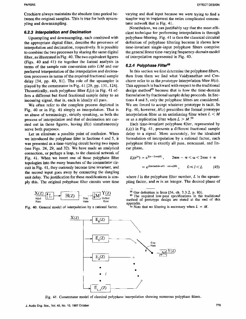
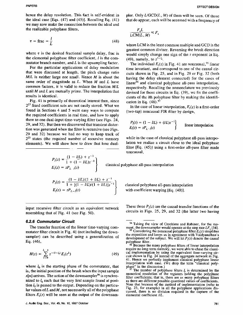
6.2.3 Interpolation and Decimation Upsampling and downsampling, each combined with
the appropriate digital filter, describe the processes of interpolation and decimation, respectively. It is possible to combine the two processes by sharing the same digital filter, as illustrated in Fig. 40. The two equivalent figures (Figs. 40 and 41) tie together the formal analysis in terms of the sample rate conversion ratio L/M and our preferred interpretation of the interpolation and decima- tion processes in terms of the required fractional sample delay [34, pp. 40, 81]. The role of the upsampler is played by the commutator in Fig. 41 [29, pp. 131,124]. Theoretically, each polyphase filter El(Z) in Fig. 41 of- fers a different but fixed fractional sample delay to an incoming signal, that is, each is ideally all pass.
We often refer to the complete process depicted in Fig. 40 or in Fig. 41 simply as interpolation. That is an abuse of terminology, strictly speaking, as both the process of interpolation and that of decimation are car- ried out in those figures, having H(z) simultaneously serve both purposes.
Let us eliminate a possible point of confusion. When we introduced the polyphase filter in Sections 4 and 5, it was presented as a time-varying circuit having two inputs (see Figs. 24, 29, and 32). We have made an analytical connection, or perhaps a leap, to the classical network of Fig. 41. When we insert one of those polyphase filter topologies into the many branches of the commutator cir- cuit in Fig. 41, they curiously become time invariant, and the second input goes away by connecting the dangling unit delay. The justification for these modifications is sim- ply this. The original polyphase filter circuits were time
varying and dual input because we were trying to find a simpler way to implement the entire complicated commu- tator network that is Fig. 41.
Nonetheless, we can justifiably say that the most effi- cient technique for performing interpolation is through polyphase filtering. Fig. 41 is then the classical circuital definition of polyphase filtering because it shows how time-invariant single-input polyphase filters comprise the general linear time-varying frequency-domain model of interpolation represented in Fig. 40.
6.2.4 Polyphase Filter sa In this section we first determine the polyphase filters,
then from them we find what Vaidyanathan and Cro- chiere refer to as the prototype interpolation filter H(z). This approach is backward with respect to the traditional design method 89 because that is how the time-domain formulation by fractional sample delay proceeds. In Sec- tions 4 and 5, only the polyphase filters are considered. We are forced to accept whatever prototype is tacit. In Fig. 40, however, H(z) prescribes the formal prototype interpolation filter as an antialiasing filter when L < M or as a replication filter when L > M. 9~
Each time-invariant polyphase filter, represented by E~(z) in Fig. 41, presents a different fractional sample delay to a signal. More accurately, for the idealized formulation of interpolation by a rational factor, each polyphase filter is exactly all pass, noncausal, and lin- ear phase,
El(ej~o) = ej(o~-2~n)t/L, 2~rm -- ~r < to < 2axm + ~r
= eJZarctan[sin ~o/(1 + cos ~)]VL, 0 ~< 1 < L (45)
where l is the polyphase filter number, L is the upsam- piing factor, and m is an integer. The desired phase of
Input Output Rate Rate Rate
Fig. 40. General model of interpolation by a rational factor.
ss Our definition is from [34, ch. 3.3.2, p. 80]. 89 The required low-pass specifications in the traditional
method of prototype design are stated at the end of this appendix.
90 Note that no filtering is necessary when L = M.
X(z) . Eo(Z )
E,(z)
- - ~ E2(Z)
\ , a te
w
o
I �9
�9 1
-] EL.I(Z)
Fig. 41. Commutator model of classical polyphase interpolation showing numerous polyphase filters.
J. Audio Eng. Soc., Vol. 45, No. 10, 1997 October 779
DATTORRO PAPERS
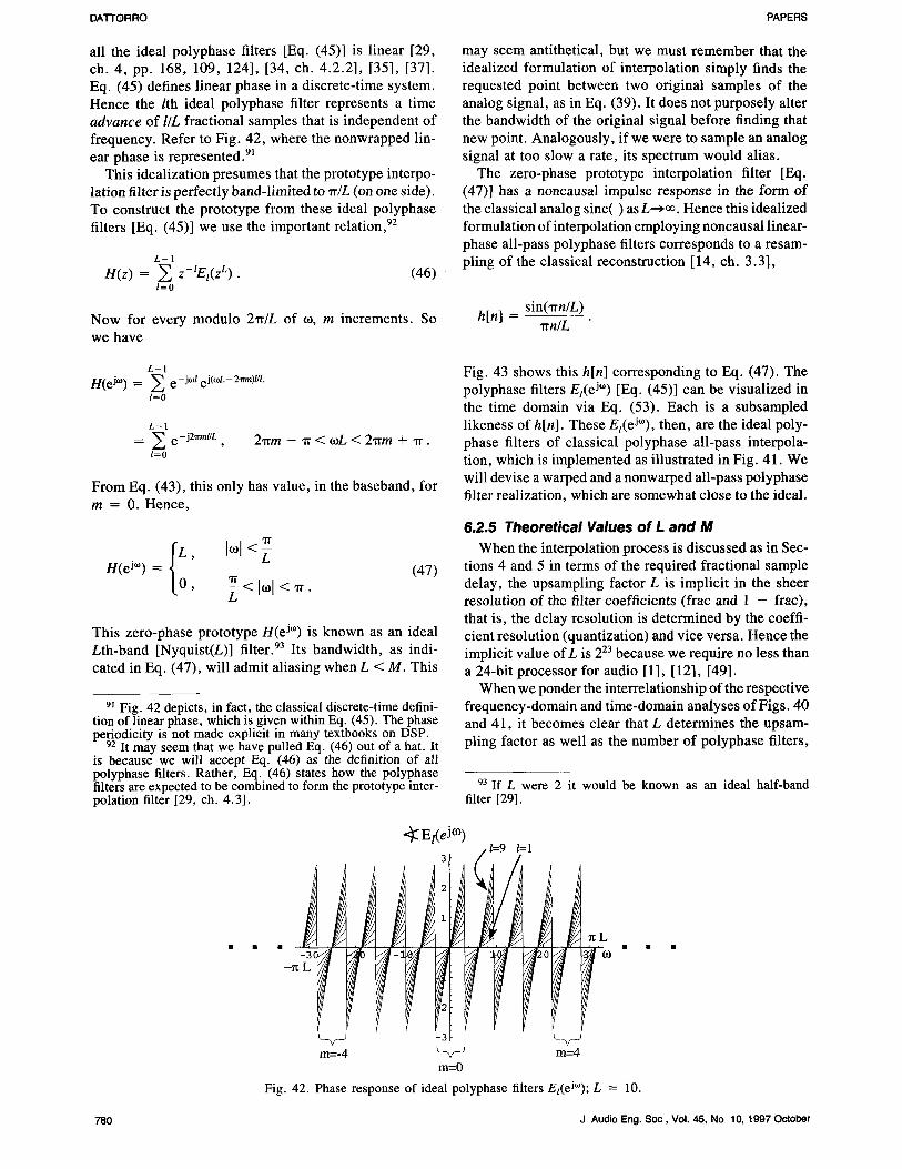
all the ideal polyphase filters [Eq. (45)] is linear [29, ch. 4, pp. 168, 109, 124], [34, ch. 4.2.2], [35], [37]. Eq. (45) defines linear phase in a discrete-time system. Hence the /th ideal polyphase filter represents a time advance of l/L fractional samples that is independent of frequency. Refer to Fig. 42, where the nonwrapped lin- ear phase is represented. 9~
This idealization presumes that the prototype interpo- lation filter is perfectly band-limited to w/L (on one side). To construct the prototype from these ideal polyphase filters [Eq. (45)] we use the important relation, 92
L - 1
n(z) = E Z-IEI(zL)" (46) / = 0
Now for every modulo 2~r/L of co, m increments. So we have
may seem antithetical, but we must remember that the idealized formulation of interpolation simply finds the requested point between two original samples of the analog signal, as in Eq. (39). It does not purposely alter the bandwidth of the original signal before finding that new point. Analogously, if we were to sample an analog signal at too slow a rate, its spectrum would alias.
The zero-phase prototype interpolation filter [Eq. (47)] has a noncausal impulse response in the form of the classical analog sinc( ) as L--->oo. Hence this idealized formulation of interpolation employing noncausal linear- phase all-pass polyphase filters corresponds to a resam- piing of the classical reconstruction [14, ch. 3.3],
sin('rrn/L ) h[n] -
,rrn/L
L - I H(O '~) = ~ e-J=le j(~
l = 0
L - 1 ~--" Z e-J2"mn//L '
l=0 2~rm - "tr < coL < 2~m + -rr.
From Eq. (43), this only has value, in the baseband, for m = 0. Hence,
'17
H(eJ•) = ' ~ < IcoI < ~ .
L
(47)
This zero-phase prototype H(e j'~ is known as an ideal Lth-band [Nyquist(L)] filter. 93 Its bandwidth, as indi- cated in Eq. (47), will admit aliasing when L < M. This
91 Fig. 42 depicts, in fact, the classical discrete-time defini- tion of linear phase, which is given within Eq. (45). The phase periodicity is not made explicit in many textbooks on DSP.
92 It may seem that we have pulled Eq. (46) out of a hat. It is because we will accept Eq. (46) as the definition of all polyphase filters. Rather, Eq. (46) states how the polyphase filters are expected to be combined to form the prototype inter- polation filter [29, ch. 4.3].
Fig. 43 shows this h[n] corresponding to Eq. (47). The polyphase filters Ej(e j~ [Eq. (45)] can be visualized in the time domain via Eq. (53). Each is a subsampled likeness of h[n]. These El(e J~ then, are the ideal poly- phase filters of classical polyphase all-pass interpola- tion, which is implemented as illustrated in Fig. 41. We will devise a warped and a nonwarped all-pass polyphase filter realization, which are somewhat close to the ideal.
6.2.5 Theoretical Values of L and M When the interpolation process is discussed as in Sec-
tions 4 and 5 in terms of the required fractional sample delay, the upsampling factor L is implicit in the sheer resolution of the filter coefficients (frac and 1 - frac), that is, the delay resolution is determined by the coeffi- cient resolution (quantization) and vice versa. Hence the implicit value of L is 223 because we require no less than a 24-bit processor for audio [1], [12], [49].
When we ponder the interrelationship of the respective frequency-domain and time-domain analyses of Figs. 40 and 41, it becomes clear that L determines the upsam- piing factor as well as the number of polyphase filters,
93 If L were 2 it would be known as an ideal half-band filter [29].
-9
/ l=9 l=1 <~ E/(eJco)
3
2
2
- 3
m = O
1 1
m=-4 m--4
.~L
Fig. 42. Phase response of ideal polyphase filters El(eJ~'); L = 10.
780 J Audio Eng. Soc, Vol. 45, No 10, 1997 October
PAPERS EFFECT DESIGN
hence the delay resolution. This fact is self-evident in the ideal case [Eqs. (47) and (45)]. Recalling Eq. (41) we may now make the connection between the ideal and the realizable polyphase filters,
l "r = frac = ~, (48)
where �9 is the desired fractional sample delay, frac is the elemental polyphase filter coefficient, l is the com- mutator branch number, and L is the upsampling factor.
For the particular applications of delay modulation that were discussed at length, the pitch change ratio M/L is neither large nor small. Hence M is about the same order of magnitude as L. When M and L have common factors, it is valid to reduce the fraction M/L until M and L are mutually prime. The interpolation that results is identical.
Fig. 41 is primarily of theoretical interest then, since 2 z3 fixed coefficient sets are not easily stored. What we found in Sections 4 and 5 were easy ways to compute the required coefficients in real time, and how to apply them to one dual-input time-varying filter (see Figs. 24, 29, and 32). But then we discovered that transient distor- tion was generated when the filter is recursive (see Figs. 29 and 32) because we had no way to keep track of 2 z3 states (the required number of recursive memory elements). We will show how to draw that lone dual-
pl(Z)~_. ~l_]__'--(f/t) -]-z-l.] El(z) ZpL_t(Z)-- I/L)z-1 1
pier. Only L/GCD(L, M) of them will be seen. Of those that do appear, each will be accessed with a frequency of
FsL <~ F s
LCM(L, M)
where LCM is the least common multiple and GCD is the greatest common divisor. Reversing the brush direction would simply change one sign of the z exponent in Eq. (49), namely, to z l-t0.
The individual Et(z ) in Fig. 41 are noncausal, 95 linear time invariant, and correspond to one of the causal cir- cuits shown in Fig. 25, and in Fig. 29 or Fig. 32 (both having the delay element connected) for the cases of linear 96 and classical polyphase all-pass interpolation, respectively. Recalling the nomenclature we previously devised for those circuits in Eq. (39), we fix the coeffi- cients of the/ th polyphase filter by making the identifi- cation in Eq. ( 4 8 ) . 97
In the case of linear interpolation, El(Z ) is a first-order (two-tap) noncausal FIR filter by design,
Pl(Z) = (1 - l/L) + (l/Z)z-l~ El(Z ) = ZPL_I(Z ) J
linear interpolation
while in the case of classical polyphase all-pass interpo- lation we realize a circuit close to the ideal polyphase filter [Eq. (45)] using a first-order all-pass filter made noncausal,
classical polyphase all-pass interpolation
( 1 - l/L)/(1 + I/L) + z-~ .~ Pt(z) = 1 + [(1 - l/L)/(1 + l/L)]z-~[
Et(z) zPL- t(z) J classical polyphase all-pass interpolation with coefficient warping [Eq. (40)].
input recursive filter circuit as an equivalent network resembling that of Fig. 41 (see Fig. 50).
6.2.6 Commutator Circuit The transfer function of the linear time-varying com-
mutator filter circuit in Fig. 41 (not including the down- sampler) can be described using a generalization of Eq. (46),
L-I H(z) = ~ z -(t-t~ Et(z L) (49)
1=o
where l 0 is the starting phase of the commutator, that is, the initial position of the brush when the input sample x[n] arrives. The action of the downsampler 94 is synchro- nized to l 0 such that the very first sample found at posi- tion 10 is passed to the output. Depending on the particu- lar values of L and M, not necessarily all of the polyphase filters El(Z) will be seen at the output of the downsam-
These three Pt(z) are the causal transfer functions of the circuits in Figs. 25, 29, and 32 (the latter two having
94 Taking the view of Crochiere and Rabiner, for the mo- ment, the downsampler would operate at the step rate LF s [34].
95 Considering the noncausal polyphase filter Ej(z) simplifies the exposition and keeps us in agreement with Vaidyanathan's development of the subject. We will let Pt(z) denote the causal polyphase filter.
96 Because the many polyphase filters of linear interpolation require no long-term memory, we were able to cheat the classi- cal implementation by using the equivalent time-varying cir- cuit shown in Fig. 24 instead of the aggregate network in Fig. 41. Hence we perfectly implement classical polyphase linear interpolation with ease. (We drop the term "classical poly- phase" in the discussion.)
97 The number of polyphase filters L is determined by the numerical resolution of the registers holding the polyphase filter coefficients; that is, there are as many polyphase filters as there are different possible quantized values of coefficients. Note that because of the method of implementation (refer to Fig. 23, for example) in all the polyphase applications dis- cussed, there is no division required in the capture of the elemental coefficient l/L.
J. Audio Eng. Soc, Vol. 45, No. 10, 1997 October 781
DATTORRO PAPERS
the delay element connected) [44, p. 178], [39, p. 50]. All three transfers are time invariant when the corres- ponding circuits are inserted into the / th branch of the commutator circuit in Fig. 41.
We reverse the order of the index in Pz(z) via the substitution l--*L - l because the polyphase filters El(z) in Fig. 41 are ordered by increasing time advance, whereas the Pl(z) are ordered by increasing delay.
The ideal Et(z) are noncausal [Eq. (45)]. This warrants multiplication of the various first-order causal PL_I(Z) by z so that the impulse response of each corresponding prototype filter Eq. (46) is time aligned with the others (see Figs. 43-46) . But this analytical z factor is unneces- sary when realizing an implementation.
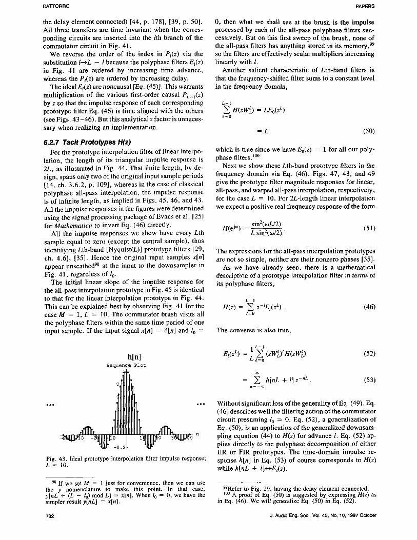
6.2.7 Tacit Prototypes H(z) For the prototype interpolation filter of linear interpo-
lation, the length of its triangular impulse response is 2L, as illustrated in Fig. 44. That finite length, by de- sign, spans only two of the original input sample periods [14, ch. 3.6.2, p. 109], whereas in the case of classical polyphase all-pass interpolation, the impulse response is of infinite length, as implied in Figs. 45, 46, and 43. All the impulse responses in the figures were determined using the signal processing package of Evans et al. [25] for Mathematica to invert Eq. (46) directly.
All the impulse responses we show have every Lth sample equal to zero (except the central sample), thus identifying Lth-band [Nyquist(L)] prototype filters [29, ch. 4.6], [35]. Hence the original input samples x[n] appear unscathed 98 at the input to the downsampler in Fig. 41, regardless of l 0.
The initial linear slope of the impulse response for the all-pass interpolation prototype in Fig. 45 is identical to that for the linear interpolation prototype in Fig. 44. This can be explained best by observing Fig. 41 for the case M = 1, L = I0. The commutator brush visits all the polyphase filters within the same time period of one input sample. If the input signal x[n] = ~[n] and l 0 =
h[n] Sequence Plot
i = = w n m
n
Fig. 43. Ideal prototype interpolation filter impulse response; L = 1 0 .
98 If we set M = 1 just for convenience, then we can use the y nomenclature to make this point. In that case, y[nL + (L - l o) mod L] = x[n]. When l 0 = 0, we have the simpler result y[nL] = x[n].
0, then what we shall see at the brush is the impulse processed by each of the all-pass polyphase filters suc- cessively. But on this first sweep of the brush, none of the all-pass filters has anything stored in its memory, 99 so the filters are effectively scalar multipliers increasing linearly with I.
Another salient characteristic of Lth-band filters is that the frequency-shifted filter sums to a constant level in the frequency domain,
L-1 H(zW~) = t, Eo(Z L)
k=O
= L (50)
which is true since we have Eo(z) = 1 for all our poly- phase filters, m0
Next we show these Lth-band prototype filters in the frequency domain via Eq. (46). Figs. 47, 48, and 49 give the prototype filter magnitude responses for linear, all-pass, and warped all-pass interpolation, respectively, for the case L = 10. For 2L-length linear interpolation we expect a positive real frequency response of the form
H(e j=) = sinZ(~ L sin2(to/2) " (51)
The expressions for the all-pass interpolation prototypes are not so simple, neither are their nonzero phases [35].
As we have already seen, there is a mathematical description of a prototype interpolation filter in terms of its polyphase filters,
L- I H(z) = ~ z-tEt(zL). (46)
l=0
The converse is also true,
1 L - I EI('Z. L) = L ~ (zWk) 1 H(zWkL)
~ = o
(52)
= ~ h[nL + l]z -"L. (53) n = - - c o
Without significant loss of the generality of Eq. (49), Eq. (46) describes well the filtering action of the commutator circuit presuming l 0 --- 0. Eq. (52), a generalization of Eq. (50), is an application of the generalized downsam- piing equation (44) to H(z) for advance I. Eq. (52) ap- plies directly to the polyphase decomposition of either IIR or FIR prototypes. The time-domain impulse re- sponse h[n] in Eq. (53) of course corresponds to H(z) while h[nL + l]<--~El(z).
99Refer to Fig. 29, having the delay element connected. 100 A proof of Eq. (50) is suggested by expressing H(z) as
in Eq. (46). We will generalize Eq. (50) in Eq. (52).
782 J. Audio Eng. Soc, Vol. 45, No. 10, 1997 October
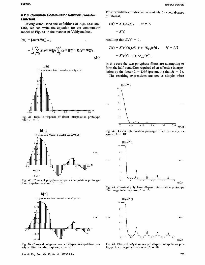
PAPERS EFFECT DESIGN
6.2.8 Complete Commutator Network Transfer Function
Having established the definitions o f Eqs. (52) and (46), we can write the equation for the commutator model o f Fig. 41 in the manner o f Vaidyanathan,
Y(z) = [X(z L) H(z)] ,~ M
M - 1 L - I
1 Z X(zL/M WMb") s (zllM W~)-I El(zL/M WMbn)" M m=o /=o
(54)
h[n] Discrete-Time Domain Analysis
i,
r011 Iillr , oT] T . . . . . . . . . . . . . . . . . . . . . . . . . . . . . . . n
-i0 i0 20 30 40
Fig. 44. Impulse response of linear interpolation prototype filter; L = 10.
h[n] Discrete-Time Domain Analysis ,,,tl] IIlo
m=a
_, _ _.,,TTTTTT__
- 0 . 4
Fig. 45. Classical polyphase all-pass interpolation prototype filter impulse response; L -- 10.
h[n] Discrete-Time Domain Analysis ,11 llIIIll[~
R i B
_,TII __..,Till] . . . .
- 0 . 4
Fig. 46. Classical polyphase warped all-pass interpolation pro- totype filter impulse response; L = 10.
This formidable equation reduces nicely for special cases of interest,
Y(z) = X ( z ) E o ( z ) , M = L
= X ( z )
recalling that Eo(z) = 1.
1 2 Y(z) = X(z2 ) [Eo( z 2) Jr z - EL/2(Z )] , M = L / 2
---- X(a2 ) [1 + z-IEL/2(Z2)] .
In this case the two polyphase filters are attempting to form the half-band filter required of an effective interpo- lation by the factor 2 = L / M (pretending that M = 1).
The resulting expressions are not as simple when
H(eJ m) 10
8
i m l 6 mlm
4
2
0 0 . 1 0 2 0 3 0 . 4 0 . 5 m/2r~
Fig. 47. Linear interpolation prototype filter frequency re- sponse; L = 10.
IH(eJm)l 10 ------~
8 -
6
0.i 02 03 04 05 m/2n
Fig. 48. Classical polyphase all-pass interpolation prototype filter magnitude response; L = 10.
IH(eJm)l 10
8
6
4
0 . 1 .A.
0 . 2 03 A j ~ . _ ,
04 05 m/2~
Fig. 49. Classical polyphase warped all-pass interpolation pro- totype filter magnitude response; L = 10.
J. Audio Eng Soc., Vol. 45, No. 10, 1997 October 783
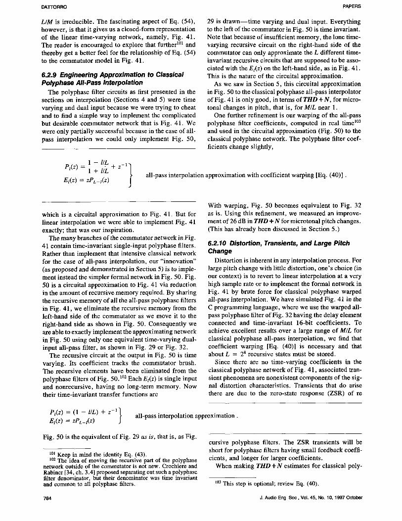
DATTORRO PAPERS
L/M is irreducible. The fascinating aspect of Eq. (54), however, is that it gives us a closed-form representation of the linear time-varying network, namely, Fig. 41. The reader is encouraged to explore that further ~~ and thereby get a better feel for the relationship of Eq. (54) to the commutator model in Fig. 41.
6.2.9 Engineering Approximation to Classical Polyphase All-Pass Interpolation
The polyphase filter circuits as first presented in the sections on interpolation (Sections 4 and 5) were time varying and dual input because we were trying to cheat and to find a simple way to implement the complicated but desirable commutator network that is Fig. 41. We were only partially successful because in the case of all- pass interpolation we could only implement Fig. 50,
29 is d rawn-- t ime varying and dual input. Everything to the left of the commutator in Fig. 50 is time invariant. Note that because of insufficient memory, the lone time- varying recursive circuit on the right-hand side of the commutator can only approximate the L different time- invariant recursive circuits that are supposed to be asso- ciated with the E l ( Z ) o n the left-hand side, as in Fig. 41. This is the nature of the circuital approximation.
As we saw in Section 5, this circuital approximation in Fig. 50 to the classical polyphase all-pass interpolator of Fig. 41 is only good, in terms of T H D + N , for micro- tonal changes in pitch, that is, for M/L near 1.
One further refinement is our warping of the all-pass polyphase filter coefficients, computed in real time ~~ and used in the circuital approximation (Fig. 50) to the classical polyphase network. The polyphase filter coef- ficients change slightly,
pt(z ) _ 1 - l/L + z_l] 1 + l/L
E l ( Z ) = zPL-I(Z) all-pass interpolation approximation with coefficient warping [Eq. (40)].
which is a circuital approximation to Fig. 41. But for linear interpolation we were able to implement Fig. 41 exactly; that was our inspiration.
The many branches of the commutator network in Fig. 41 contain time-invariant single-input polyphase filters. Rather than implement that intensive classical network for the case of all-pass interpolation, our "innovation" (as proposed and demonstrated in Section 5) is to imple- ment instead the simpler formal network in Fig. 50. Fig. 50 is a circuital approximation to Fig. 41 via reduction in the amount of recursive memory required. By sharing the recursive memory of all the all-pass polyphase filters in Fig. 41, we eliminate the recursive memory from the left-hand side of the commutator as we move it to the right-hand side as shown in Fig. 50. Consequently we are able to exactly implement the approximating network in Fig. 50 using only one equivalent time-varying dual- input all-pass filter, as shown in Fig. 29 or Fig. 32.
The recursive circuit at the output in Fig. 50 is time varying. Its coefficient tracks the commutator brush. The recursive elements have been eliminated from the polyphase filters of Fig. 50.1~ Each El(Z) is single input and nonrecursive, having no long-term memory. Now their time-invariant transfer functions are
With warping, Fig. 50 becomes equivalent to Fig. 32 as is. Using this refinement, we measured an improve- ment of 26 dB in T H D + N for microtonal pitch changes. (This has already been discussed in Section 5.)
6.2.10 Distortion, Transients, and Large Pitch Change
Distortion is inherent in any interpolation process. For large pitch change with little distortion, one's choice (in our context) is to revert to linear interpolation at a very high sample rate or to implement the formal network in Fig. 41 by brute force for classical polyphase warped all-pass interpolation. We have simulated Fig. 41 in the C programming language, where we use the warped all- pass polyphase filter of Fig. 32 having the delay element connected and time-invariant 16-bit coefficients. To achieve excellent results over a large range of M/L for classical polyphase all-pass interpolation, we find that coefficient warping [Eq. (40)] is necessary and that about L = 28 recursive states must be stored.
Since there are no time-varying coefficients in the classical polyphase network of Fig. 41, associated tran- sient phenomena are nonexistent components of the sig- nal distortion characteristics. Transients that do arise there are due to the zero-state response (ZSR) of re
Pl(Z) = (1 - l/L) + z - l ~
El(Z) ZPL-I(Z) J all-pass interpolation approximation.
Fig. 50 is the equivalent of Fig. 29 as is, that is, as Fig.
101 Keep in mind the identity Eq. (43). 102 The idea of moving the recursive part of the polyphase
network outside of the commutator is not new. Crochiere and Rabiner [34, ch. 3.4] proposed separating out such a polyphase filter denominator, but their denominator was time invariant and common to all polyphase filters.
cursive polyphase filters. The ZSR transients will be short for polyphase filters having small feedback coeffi- cients, and longer for larger coefficients.
When making T H D + N estimates for classical poly-
103 This step is optional; review Eq. (40).
784 J. Audio Eng Soc, Vol. 45, No. 10, 1997 October
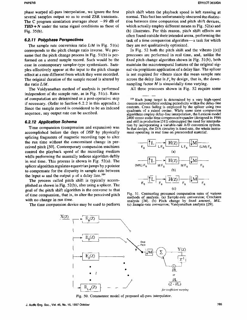
PAPERS EFFECT DESIGN
phase warped all-pass interpolation, we ignore the first several samples output so as to avoid ZSR transients. The C program simulation averages about - 8 9 dB of TItD + N under the same signal conditions as those of Fig. 35(b).
6.2.11 Polyphase Perspectives The sample rate conversion ratio L/M in Fig. 51(a)
corresponds to the pitch change ratio inverse. We pre- sume that the pitch change process in Fig. 51(b) is per- formed on a stored sample record. Such would be the case in contemporary sampler-type synthesizers. Sam- ples effectively appear at the input to the pitch change effect at a rate different from which they were recorded. The original duration of the sample record is altered by the ratio L/M.
The Vaidyanathan method of analysis is performed independent of the sample rate, as in Fig. 51(c). Rates of computation are determined as a post-operative step if necessary. (Refer to Section 6.2.2 in this appendix.) Since the sample record is considered to be an indexed sequence, any output rate can be ascribed.
6.2.12 Application Schema Time compansion (compression and expansion) was
accomplished before the days of DSP by physically splicing fragments of magnetic recording tape to alter the run time without the concomitant change in per- ceived pitch [50]. Contemporary compansion machines control the playback speed of the recording medium while performing the manually tedious algorithm deftly in real time. This process is shown in Fig. 52(a). The splicer algorithm regulates equestrian jumps by p pointer to compensate for the disparity in sample rate between the input to and the output p of a delay line.t~
The process called pitch shift is typically accom- plished as shown in Fig. 52(b), also using a splicer. The goal of the pitch shift algorithm is the converse to that of time compansion, that is, to alter the perceived pitch with no change in run time.
The time compansion device may be used to perform
pitch shift when the playback speed is left running a t
normal. This fact has unfortunately obscured the distinc- tion between time compansion and pitch shift devices, which actually employ different means as Fig. 52(a) and (b) illustrates. For this reason, pitch shift effects are often found outside their intended arena, performing the task of a time compansion algori thm--a task for which they are not qualitatively optimized.
In Fig. 52 both the pitch shift and the vibrato [(c)] processes are performed in real time, and, unlike the fixed pitch change algorithm shown in Fig. 51 (b), both maintain the macrotemporal features of the original sig- nal via propitious application of a delay line. The splicer is not required for vibrato since the mean sample rate across the delay line is F s by design, that is, the down- sampling factor M is sinusoidally time varying.
All three processes shown in Fig. 52 require some
104 Each jump target is determined by a very high-speed custom autocorrelator seeking periodicity within the delay-line contents. Cross fading is employed by the splicer using two quadrants of a raised cosine. While some time compansion algorithms employ delay-line interpolation, the Lexicon model 2400 stereo audio time compressor/expander (designed in 1986 and still in production [51 ]) sidestepped the need for interpola- tion by incorporating a variable-rate A/D conversion system. In that design, the D/A circuitry is fixed rate, the whole instru- ment operating in real time on prerecorded material.
F s ~---~ LFs ' ' LFs ~---~ (L/M) F s (a)
(M/L) F s ~ F s (h)
Fs ~ Fs
(c) Fig. 51. Contrasting presumed computation rates of various methods of analysis. (a) Sample-rate conversion; Crochiere analysis [34]. (b) Pitch change by fixed amount, M/L. (c) Sample-rate conversion; Vaidyanathan analysis [29].
X(z) �9 E~ t
----~ El(Z) t
- - - ~ E2(Z) [
�9 l
EL-I(Z) }
\ ""•o• Step
| �9 l/L
�9 Or
(2 - l/L) for coefficient warping
Fig. 50. Commutator model of proposed all-pass interpolator.
J. Audio Eng. Soc., Vol. 45, No. 10, 1997 October 785
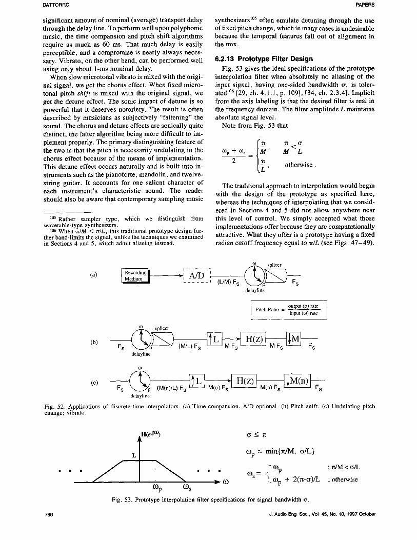
DA'I-I'OR RO PAPERS
significant amount of nominal (average) transport delay through the delay line. To perform well upon polyphonic music, the time compansion and pitch shift algorithms require as much as 60 ms. That much delay is easily perceptible, and a compromise is nearly always neces- sary. Vibrato, on the other hand, can be performed well using only about 1-ms nominal delay.
When slow microtonal vibrato is mixed with the origi- nal signal, we get the chorus effect. When fixed micro- tonal pitch shift is mixed with the original signal, we get the detune effect. The sonic impact of detune is so powerful that it deserves notoriety. The result is often described by musicians as subjectively "fattening" the sound. The chorus and detune effects are sonically quite distinct, the latter algorithm being more difficult to im- plement properly. The primary distinguishing feature of the two is that the pitch is necessarily undulating in the chorus effect because of the means of implementation. This detune effect occurs naturally and is built into in- struments such as the pianoforte, mandolin, and twelve- string guitar. It accounts for one salient character of each instrument's characteristic sound. The reader should also be aware that contemporary sampling music
105 Rather sampler type, which we distinguish from wavetable-type synthesizers.
106 When ~r/M < tr/L, this traditional prototype design fur- ther band-limits the signal, unlike the techniques we examined in Sections 4 and 5, which admit aliasing instead.
synthesizers ms often emulate detuning through the use of fixed pitch change, which in many cases is undesirable because the temporal features fall out of alignment in the mix.
6.2.13 Prototype Filter Design Fig. 53 gives the ideal specifications of the prototype
interpolation filter when absolutely no aliasing of the input signal, having one-sided bandwidth tr, is toler- ated 1~ [29, ch. 4.1.1, p. 109], [34, ch. 2.3.4]. Implicit from the axis labeling is that the desired filter is real in the frequency domain. The filter amplitude L maintains absolute signal level.
Note from Fig. 53 that
M "rr <_~ tOp q- tos -- ' M L
2 I~L ' otherwise.
The traditional approach to interpolation would begin with the design of the prototype as specified here, whereas the techniques of interpolation that we consid- ered in Sections 4 and 5 did not allow anywhere near this level of control. We simply accepted what those implementations offer because they are computationally attractive. What they offer is a prototype having a fixed radian cutoff frequency equal to w/L (see Figs. 47-49).
CO splicer [ Recording ~ ~: . . . . . ~ ~ ! ~ - ' )
(a) Medium | -~ __A/D__ ,j (L/M) F s ~ F s
delayline
(b)
Pitch Ratio output (p) rate input (m) rate
splicer
delayline
CO
(c) Fs ~ (M(n)/L)Fs ~ M(n) F ~ ] ~ H T ~ M(n) Fs m(n)'s delayline
Fig. 52. Applications of discrete-time interpolators. (a) Time companslon. A/D optional (b) Pitch shift. (c) Undulating pitch change; vibrato.
. . . f HceJ~ (~ < n
L COp - min { n/M, t~/L }
{ COp ; ~ M < ~/L �9 �9 �9 COS ----
03 ~ COp + 2(rc-~)/L ;otherwise 03p COs
Fig. 53. Prototype interpolation filter specifications for signal bandwidth tr.
786 J. Audio Eng Soc., Vol 45, No. 10, 1997 October
PAPERS EFFECT DESIGN
REFERENCES
[1] D. C. Andreas, J. Dattorro, and J. W. Mauchly, "Digital Signal Processor for Audio Applications," U.S. patent 5,517,436 (1996 May 14).
[2] W. G. Gardner, "Reverberation Algorithms," in Applications of Signal Processing to Audio and Acous- tics, M. Kahrs and K. Brandenburg, Eds. (Kluwer Aca- demic, Norwell, MA, 1997).
[3] J. A. Moorer, "About this Reverberation Busi- ness," Computer Music J., vol. 3, pp. 13-28 (1979 June), also in Foundations of Computer Music, C. Roads and J. Strawn, Eds. (MIT Press, Cambridge, MA, 1988).
[4] D. Griesinger, "Practical Processors and Pro- grams for Digital Reverberation," in Audio in Digital Times, Proc. Audio Eng. Soc. 7th Int. Conf. (Toronto, Ont., Canada, 1989 May 14-17), pp. 187-195.
[5] B. A. Blesser and K. O. Bader, "Electric Reverber- ation Apparatus," U.S. patent 4,181,820 (1980 Jan. 1).
[6] D. Griesinger, "Room Impression, Reverberance, and Warmth in Rooms and Halls," presented at the 93rd Convention of the Audio Engineering Society, J. Audio Eng. Soc. (Abstracts), vol. 40, p. 1064 (1992 Dec.), preprint 3383.
[7] M. Schroeder, "Natural Sounding Artificial Re- verberation," J. Audio Eng. Soc., vol. 10, p. 219 (1962 July).
[8] J. M. Jot and A. Chaigne, "Digital Delay Net- works for Designing Artificial Reverberators," presented at the 90th Convention of the Audio Engineering Soci- ety, J. Audio Eng. Soc. (Abstracts), vol. 39, p. 383 (1991 May), preprint 3030.
[9] J. O. Smith, "Elimination of Limit Cycles and Overflow Oscillations in Time-Varying Lattice and Lad- der Digital Filters," in Music Applications of Digital Waveguides, Rep. STAN-M-39, Center for Computer Research in Music and Acoustics (CCRMA), Dept. of Music, Stanford University, Stanford, CA (1987 May).
[10] A. V. Oppenheim, Ed., Applications of Digital Signal Processing (Prentice-Hall, Englewood Cliffs, NJ, 1978).
[11] L. B. Jackson, Digital Filters and Signal Pro- cessing, 3rd ed. (Kluwer Academic, Norwell, MA, 1996).
[12] J. Dattorro, "The Implementation of Recursive Digital Filters for High-Fidelity Audio," J. Audio Eng. Soc., vol. 36, pp. 851-878 (1988 Nov.); Comments, ibid. (Letters to the Editor), vol. 37, p. 486 (1989 June); Comments, ibid. (Letters to the Editor), vol. 38, pp. 149-151 (1990 Mar.).
[13] P. A. Regalia and S. K. Mitra, "Tunable Digital Frequency Response Equalization Filters," IEEE Trans. Acoust., Speech, Signal Process., vol. ASSP-35, pp. 118-120 (1987 Jan.).
[14] A. V. Oppenheim and R. W. Schafer, Discrete- Time Signal Processing (Prentice-Hall, Englewood Cliffs, NJ, 1989).
[15] J. Strawn, Ed., Digital Audio Signal Processing
(A-R Editions, Madison, WI, 1985). [ 16] J. A. Moorer, "The Mafiifold Joys of Conformal
Mapping: Applications to Digital Filtering in the Stu- dio," J. Audio Eng. Soc., vol. 31, pp. 826-841 (1983 Nov.).
[17] D. P. Rossum, "Dynamic Digital IIR Audio Fil- ter and Method which Provides Dynamic Digital Filter- ing for Audio Signals," U.S. patent 5,170,369 (1992 Dec.).
[18] T. I. Laakso, "Error Feedback for Reduction of Quantization Errors due to Arithmetic Operations in Re- cursive Digital Filters," D. Tech. thesis, Rep. 9, Labora- tory of Signal Processing and Computer Technology, Helsinki University of Technology, Espoo, Finland (1991).
[ 19] K. Steiglitz, A Digital Signal Processing Primer (Addison-Wesley, Menlo Park, CA, 1996).
[20] Moog Voltage-Controlled Ladder Filter, In- ternet: http://www.sara.nl/Rick.Jansen/Emusic/Moog/ moogvcf_schematic.gif and Internet: http://www- ccrma, stanford, edu/ - stilti/papers/moogvcf, pdf.
[21] D. Rossum, "Making Digital Filters Sound 'An- alog,'" in Proc. Int. Computer Music Conf. (San Jose, CA, 1992), pp. 30-33.
[22] "CEM3328 Four Pole Low Pass VCF," Curtis Electromusic Specialties, Los Gatos, CA (1983).
[23] H. Chamberlin, Musical Applications of Micro- processors (Hayden, Indianapolis, IN, 1980).
[24] Mathematica, version 2, Wolfram Research, Champaign, IL (1994).
[25] B. L. Evans, L. J. Karam, K. A. West, and J. H. McClellan, "Learning Signals and Systems with Mathematica," IEEE Trans. Education, vol. 36, pp. 72-78 (1993 Feb.).
[26] K. W. Martin and M. T. Sun, "Adaptive Filters Suitable for Real-Time Spectral Analysis," IEEE Trans. Circuits Sys., vol. CAS-33, pp. 218-229 (1986 Feb.); also IEEE J. Solid-State Circuits, vol. SC-21, no. 1 (1986 Feb.), pp. 108-119.
[27] M. R. Petraglia, S. K. Mitra, and J. Szczupak, "Adaptive Sinusoid Detection Using IIR Notch Filters and Multirate Techniques," IEEE Trans. Circuits Sys. H, vol. 41, pp. 709-717 (1994 Nov.).
[28] T. Kwan and K. Martin, "Adaptive Detection and Enhancement of Multiple Sinusoids Using a Cascade IIR Filter," IEEE Trans. Circuits Sys., vol. 36, pp. 937-947 (1989 July).
[29] P. P. Vaidyanathan, Multirate Systems and Fil- ter Banks (Prentice-Hall, Englewood Cliffs, NJ, 1993).
[30] T. I. Laakso, P. S. R. Diniz, I. Hartimo, and T. C. Macedo, Jr., "Elimination of Zero-Input and Constant-Input Limit Cycles in Single-Quantizer Re- cursive Filter Structures," IEEE Trans. Circuits Sys. H, vol. 39, pp. 638-646 (1992 Sept.).
[31] A. Luthra, "Extension of Parseval's Relation to Nonuniform Sampling," IEEE Trans. Acoust., Speech, Signal Process., vol. 36 (1988 Dec.), pp. 1909-1911.
[32] R. W. Schafer and L. R. Rabiner, "A Digital Signal Processing Approach to Interpolation," Proc. IEEE, vol. 61, pp. 692-702 (1973 June).
J. Audio Eng. Soc., Vol 45, No 10, 1997 October 787
DA'I-I'ORRO PAPERS
[33] F. R. Moore, "Table Lookup Noise for Sinusoi- dal Digital Oscillators," Computer Music J., vol. 1, pp. 26 - 29 ( 1977 Apr.), also in Elements of Computer Music (Prentice-Hall, Englewood Cliffs, NJ, 1990), chap. 3.
[34] R. E. Crochiere and L. R. Rabiner, Multirate Digital Signal Processing (Prentice-Hall, Englewood Cliffs, NJ, 1983).
[35] M. Renfors and T. Saramiiki, "Recursive Nth- Band Digital Filters--Parts I and II," IEEE Trans. Cir- cuits Sys., vol. CAS-34, pp. 24-51 (1987 Jan.).
[36] D. Rossum, "An Analysis of Pitch Shifting Al- gorithms," presented at the 87th Convention of the Audio Engineering Society, J. Audio Eng. Soc. (Ab- stracts), vol. 37, p. 1072 (1989 Dec.), preprint 2843.
[37] R. Adams and T. Kwan, "Theory and VLSI Ar- chitectures for Asynchronous Sample-Rate Converters," J. Audio Eng. Soc., vol. 41, pp. 539-555 (1993 July/ Aug.).
[38] T. A. Ramstad, "Digital Methods for Conver- sion between Arbitrary Sampling Frequencies," IEEE Trans. Acoust., Speech, Signal Process., vol. ASSP- 32, pp. 577-591 (1984 June).
[39] T. I. Laakso, V. Viilimiiki, M. Karjalainen, and U. K. Laine, "Splitting the Unit Delay--Tools for Frac- tional Delay Filter Design," IEEE Signal Process. Mag. , vol. 13, pp. 30-60 (1996 Jan.).
[40] J. Dattorro, "The Implementation of Digital Fil- ters for High Fidelity Audio, Part I I - -FIR," in Audio in Digital Times, Proc. Audio Engineering Society 7th Int. Conf. (Toronto, ON, Canada, 1989 May 14-17), pp. 168-180.
[41] J. C. Dattorro, A. J. Charpentier, and D. C. Andreas, "Decimation Filter as for a Sigma-Delta Analog-to-Digital Converter," U.S. patent 5,027,306 (1991 June 25).
[42] D. C. Andreas, "VLSI Implementation of a One- Stage 64:1 FIR Decimator," presented at the 89th Con- vention of the Audio Engineering Society, J. Audio Eng. Soc. (Abstracts), vol. 38, p. 872 (1990 Nov.), pre- print 2976.
[43] J. O. Smith and B. Friedlander, "Adaptive, In-
terpolated Time-Delay Estimation," IEEE Trans. Aero- space Electron. Sys., vol. 21, pp. 180-199 (1985 Mar.).
[44] J. O. Smith III, "Techniques for Digital Filter Design and System Identification with Application to the Violin," Rep. STAN-M-14, Center for Computer Research in Music and Acoustics (CCRMA), Dept. of Music, Stanford University, Stanford, CA (1983 June).
[45] V. V~ilimiiki, T. I. Laakso, and J. Mackenzie, "Elimination of Transients in Time-Varying Allpass Fractional Delay Filters with Application to Digital Waveguide Modeling," in Proc. Int. Computer Music Conf. (Banff, AB, Canada, 1995), pp. 327-334.
[46] J. O. Smith, "An Allpass Approach to Digital Phasing and Flanging," Rep. STAN-M-21, Center for Computer Research in Music and Acoustics (CCRMA), Dept. of Music, Stanford University, Stanford, CA (1982 Spring).
[47] W. M. Hartmann, "Flanging and Phasers," J. Audio Eng. Soc. (Engineering Reports), vol. 26, pp. 439-443 (1978 June).
[48] M. L. Beigel, "A Digital 'Phase Shifter' for Mu- sical Applications, Using the Bell Labs (Alles-Fischer) Digital Filter Module," J. Audio Eng. Soc. (Engineering Reports), vol. 27, pp. 673-676 (1979 Sept.).
[49] DSP56000/DSP56001 Digital Signal Processor User's Manual, rev. 2 (Motorola, DSP Division, Austin, TX, 1990).
[50] F. F. Lee, "Time Compression and Expansion of Speech by the Sampling Method," J. Audio Eng. Soc., vol. 20, pp. 738-742 (1972 Nov.); also in Speech Enhancement, J. S. Lim. Ed. (Prentice-Hall, Englewood Cliffs, NJ, 1983), pp. 286-290.
[51] J. Dattorro, "Using Digital Signal Processor Chips in a Stereo Audio Time Compressor/Expander," presented at the 83rd Convention of the Audio Engi- neering Society, J. Audio Eng. Soc. (Abstracts), vol. 35, p. 1062 (1987 Dec.), preprint 2500.
The biography for Jon Dattorro was published in the 1997 September issue of the Journal.
788 J. Audio Eng Soc., Vol 45, No 10, 1997 October


![[OPTION] Professional Sampler · Power supply +5V 0.8A Effect Type List Scratch (DIGITAL SCRATCH) AutoSyn (AUTO SYNTH) TechMod (TECH MODULATION) NoisDly (NOISY MOD DELAY) NoisAmb](https://img.pdfslide.net/doc/110x75/5f36e42f8bc3163632357e28/option-professional-sampler-power-supply-5v-08a-effect-type-list-scratch-digital.jpg)