Effect of Cross-flow Momentum on Opposing Jet Mixing

Takahisa Nagao, Shinsuke Matsuno1 and A.Koichi Hayashi2

1 Research Laboratory, IHI Corporation

1, Shin-nakahara-cho, Isogo-ku, Yokohama 235-8501, Japan

E-mail: takahisa_nagao@ihi.co.jp 2 Mechanical Engineering Department, Aoyama Gakuin University, Japan

ABSTRACT

The flow of opposing jets was studied in computational fluid

dynamics simulation. To clarify the flow field of the jet engine

combustor, it is necessary to study air-jet dilution effects typical of

opposing jets. The velocity distribution and turbulence intensity

were obtained in large eddy simulation for air and an average

Reynolds number of 2 × 104 corresponding to the jet diameter and

velocity. Results obtained numerically generally agreed

quantitatively with experimental results obtained in our previous

study. Simulations were then carried out to clarify the effect of the

momentum flux ratio J (4, 9, 16, and 64) on mixing. Unmixedness

was found to be highest for J = 4 since the penetrations and thus

collision of opposing jets were weak for J = 4. When J = 9, 16, 64,

mixing was improved by jet collision. It is proposed that the mixing

mechanisms are differed depending on J.

INTRODUCTION

The operating temperatures of combustors are being raised each

year to enhance the efficiency of gas turbine engines. It is desirable

to reduce the size and mass of a combustor, yet reducing the

combustor size negatively affects the temperature distribution at the

exit of the combustor. Turbine blades can be damaged if the exhaust

gas creates hot spots, which are areas of extremely high

temperature. Thus, the temperature distribution at the combustor

exit should be adjusted in the development of gas turbine engines.

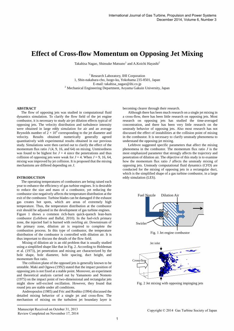
Figure 1 shows a common rich-burn quick-quench lean-burn

combustor (Lefebvre and Ballal, 2010). In the fuel-rich primary

zone, the injected fuel is burned with swirling air. Downstream of

the primary zone, dilution air is required to complete the

combustion process. In this type of combustor, the temperature

distribution of the combustor is controlled with dilution air. It is

thus important to discuss the details of the flow field.

Mixing of dilution air is an old problem that is usually studied

using a simplified shape like that in Fig. 2. According to Holdeman

et al. (1973), jet penetration and mixing are characterized by the

hole shape, hole diameter, hole spacing, duct height, and

momentum flux ratio.

The collision plane of the opposed jets is generally known to be

unstable. Maki and Ogawa (1992) stated that the impact position of

opposing jets is not fixed at a stable point. Moreover, an experiment

and theoretical analysis carried out by Yamamoto and Nomoto

(1975) on the impact point of two-dimensional and rectangular jets

might show self-excited oscillation. However, they found that

round jets are stable under all conditions.

Andreopoulos (1985) and Fric and Roshko (1994) discussed the

detailed mixing behavior of a single jet and cross-flow. The

mechanism of mixing on the turbulent jet boundary layer is

becoming clearer through their research.

Although there has been much research on a single jet mixing in

a cross-flow, there has been little research on opposing jets. Most

research on opposing jets has studied the time-averaged

concentration, and there has been very little research on the

unsteady behavior of opposing jets. Also most research has not

discussed the effect of instabilities at the collision point of mixing

in the combustor. It is necessary to clarify unsteady phenomena to

understand the opposing-jet mixing.

Lefebvre suggested specific parameters that affect the mixing

phenomena in the combustor. The momentum flux ratio J is the

most emphasized parameter that strongly affects the trajectory and

penetration of dilution air. The objective of this study is to examine

how the momentum flux ratio J affects the unsteady mixing of

opposing jets. Unsteady computational fluid dynamics (CFD) are

conducted for the mixing of opposing jets in a rectangular duct,

which is the simplified shape of a gas turbine combustor, in a large

eddy simulation (LES).

Dilution Air

Swirler

Fuel Nozzle

Fig. 1 Jet engine combustor

Fig. 2 Jet mixing with opposing impinging jets

Jet inlet

Cross-flow

International Journal of Gas Turbine, Propulsion and Power Systems December 2014, Volume 6, Number 3

Copyright © 2014 Gas Turbine Society of JapanManuscript Received on October 31, 2013 Review Completed on November 17, 2014

1

GEOMETRY

Figure 3 depicts the outline of the flow passage. As discussed in

the previous section, the flow field consists of a rectangular duct

and opposing jets. The left side of the duct is the cross-flow inlet,

and the right side is open to the atmosphere. In this study, the

entrance angle of the jets is fixed at 90 degrees to the duct. The

entrance region length is XA for the stability of calculation.

H

S

L

XA

Vj

D

Vm

Fig. 3 Outline of the flow passage

(D = 20, L = 590, W = 100, H = 100, XA = 95, X=0: Jet inlet)

NUMERICAL METHOD

The numerical methods are presented in Table 1. The

commercial CFD code Advance Soft Front Flow Red 4.1 was used

for the LES computations. The spatially filtered Navier–Stokes

equations are

jiji

ji

j

j

i

jj

ij

j

jii uuuuxx

u

x

u

xx

p

x

uu

t

u

1

,

quuuu ijjijiij 3

2 .

The subgrid-scale (SGS) eddy viscosity was modeled using the

standard Smagorinsky model as

ijij SSC 22 .

where C is the Smagorinsky coefficient and Δ is the length scale of

the SGS turbulence. In this study, C was calculated with the

dynamic SGS model (Lilly, 1992).

The minimum numerical mesh length was 0.2 mm, and the

maximum length was 2 mm. There were 3 million grid points. The

experiment was performed in our previous work (Nagao et al.,

2012). According to the comparison between analysis and

measurement, the LES was generally in quantitative agreement

with the experiment.

Table 1 Numerical methods and mesh conditions

CFD Code AdvanceSoft Advance/FrontFlow/Red 4.1

Equation Navier-Stokes

Fluid Incompressible perfect gas

Turbulent LES dynamic SGS

Jets Inlet Random perturbations (Smirnov et al., 2001)

Cross-flow Inlet Uniform velocity

Wall Spalding law, first layer thickness = 0.2mm

Cell Unstructured

Discretization Blended 2nd-order central with 1st-order upwind(8:2)

Parallelization Region splitting (METIS), MPI-Infiniband

Number of Cells 3 Million

Grid size Min. = 0.2mm, Max. = 2mm

RESULTS AND DISCUSSION

Unmixedness

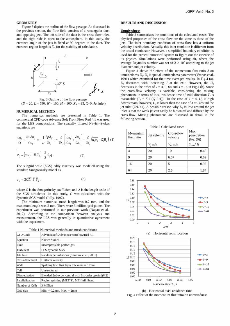
Table 2 summarizes the conditions of the calculated cases. The

physical properties of the cross-flow are the same as those of the

jets. The inlet boundary condition of cross-flow has a uniform

velocity distribution. Actually, this inlet condition is different from

the actual combustor. However, a simplified boundary condition is

used for the present numerical system to figure out the essence of

its physics. Simulations were performed using air, where the

average Reynolds number was set to 2 × 104 according to the jet

diameter and jet velocity.

Figure 4 shows the effect of the momentum flux ratio J on

unmixedness Us. Us is spatial unmixedness parameter (Vranos et al.,

1991) which examined for the time-averaged results. In Fig.4 (a),

Us decreases with increasing J at the exit. However, the Us

decreases in the order of J = 4, 9, 64 and J = 16 in Fig.4 (b). Since

the cross-flow velocity is variable, considering the mixing

phenomena in terms of local residence time of axial direction Tr is

reasonable (Tr = X / (Q / A)). In the case of J = 4, Us is high

downstream; however, Us is lower than the case of J = 9 around the

jet inlet (X/H<1). A possible reason why Us is low around the jet

inlet is that the weak jet can easily be blown off and diffused by the

cross-flow. Mixing phenomena are discussed in detail in the

following section.

Table 2 Calculated cases

Momentum

flux ratio Jet velocity

Cross-flow

velocity

Max.

penetration

(Eq. (6))

J Vj m/s Vm m/s Ymax/ H

4 20 10 0.46

9 20 6.67 0.69

16 20 5 0.92

64 20 2.5 1.84

0.00

0.02

0.04

0.06

0.08

0.10

0.12

0.14

0.16

0.18

0 1 2 3 4 5

US

X/H

J=4

J=9

J=16

J=64

(a) Horizontal axis: location

0.00

0.02

0.04

0.06

0.08

0.10

0.12

0.14

0.16

0.18

0.20

0.00 0.01 0.02 0.03 0.04 0.05

US

Residence time Tr , s

J=4

J=9

J=16

J=64

(b) Horizontal axis: residence time

Fig. 4 Effect of the momentum flux ratio on unmixedness

(1)

(2)

(3)

X

Y

Z

JGPP Vol.6, No. 3

2

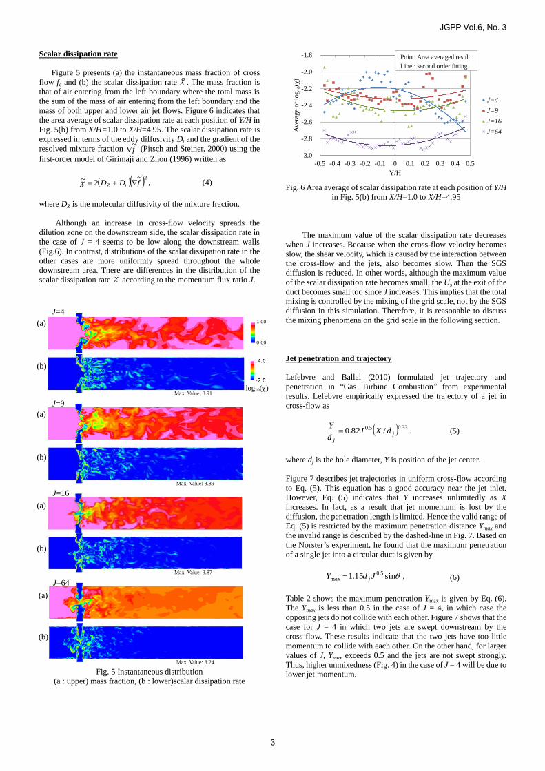
Scalar dissipation rate

Figure 5 presents (a) the instantaneous mass fraction of cross

flow fc and (b) the scalar dissipation rate 𝜒� . The mass fraction is

that of air entering from the left boundary where the total mass is

the sum of the mass of air entering from the left boundary and the

mass of both upper and lower air jet flows. Figure 6 indicates that

the area average of scalar dissipation rate at each position of Y/H in

Fig. 5(b) from X/H=1.0 to X/H=4.95. The scalar dissipation rate is

expressed in terms of the eddy diffusivity Dt and the gradient of the

resolved mixture fraction f~

(Pitsch and Steiner, 2000) using the

first-order model of Girimaji and Zhou (1996) written as

2~2~ fDD tZ ,

where DZ is the molecular diffusivity of the mixture fraction.

Although an increase in cross-flow velocity spreads the

dilution zone on the downstream side, the scalar dissipation rate in

the case of J = 4 seems to be low along the downstream walls

(Fig.6). In contrast, distributions of the scalar dissipation rate in the

other cases are more uniformly spread throughout the whole

downstream area. There are differences in the distribution of the

scalar dissipation rate 𝜒� according to the momentum flux ratio J.

Fig. 5 Instantaneous distribution

(a : upper) mass fraction, (b : lower)scalar dissipation rate

-3.0

-2.8

-2.6

-2.4

-2.2

-2.0

-1.8

-0.5 -0.4 -0.3 -0.2 -0.1 0 0.1 0.2 0.3 0.4 0.5

Av

erag

e o

f lo

g1

0(χ

)

Y/H

J=4

J=9

J=16

J=64

Fig. 6 Area average of scalar dissipation rate at each position of Y/H

in Fig. 5(b) from X/H=1.0 to X/H=4.95

The maximum value of the scalar dissipation rate decreases

when J increases. Because when the cross-flow velocity becomes

slow, the shear velocity, which is caused by the interaction between

the cross-flow and the jets, also becomes slow. Then the SGS

diffusion is reduced. In other words, although the maximum value

of the scalar dissipation rate becomes small, the Us at the exit of the

duct becomes small too since J increases. This implies that the total

mixing is controlled by the mixing of the grid scale, not by the SGS

diffusion in this simulation. Therefore, it is reasonable to discuss

the mixing phenomena on the grid scale in the following section.

Jet penetration and trajectory

Lefebvre and Ballal (2010) formulated jet trajectory and

penetration in “Gas Turbine Combustion” from experimental

results. Lefebvre empirically expressed the trajectory of a jet in

cross-flow as

33.05.0 /82.0 j

j

dXJd

Y .

where dj is the hole diameter, Y is position of the jet center.

Figure 7 describes jet trajectories in uniform cross-flow according

to Eq. (5). This equation has a good accuracy near the jet inlet.

However, Eq. (5) indicates that Y increases unlimitedly as X

increases. In fact, as a result that jet momentum is lost by the

diffusion, the penetration length is limited. Hence the valid range of

Eq. (5) is restricted by the maximum penetration distance Ymax and

the invalid range is described by the dashed-line in Fig. 7. Based on

the Norster’s experiment, he found that the maximum penetration

of a single jet into a circular duct is given by

sin15.1 5.0max JdY j ,

Table 2 shows the maximum penetration Ymax is given by Eq. (6).

The Ymax is less than 0.5 in the case of J = 4, in which case the

opposing jets do not collide with each other. Figure 7 shows that the

case for J = 4 in which two jets are swept downstream by the

cross-flow. These results indicate that the two jets have too little

momentum to collide with each other. On the other hand, for larger

values of J, Ymax exceeds 0.5 and the jets are not swept strongly.

Thus, higher unmixedness (Fig. 4) in the case of J = 4 will be due to

lower jet momentum.

(4)

log10()

(a)

(b)

(a)

(b)

(a)

(b)

(a)

(b)

Max. Value: 3.91

Max. Value: 3.89

Max. Value: 3.87

Max. Value: 3.24

(5)

(6)

J=4

J=9

J=16

J=64

Point: Area averaged result

Line : second order fitting

JGPP Vol.6, No. 3

3

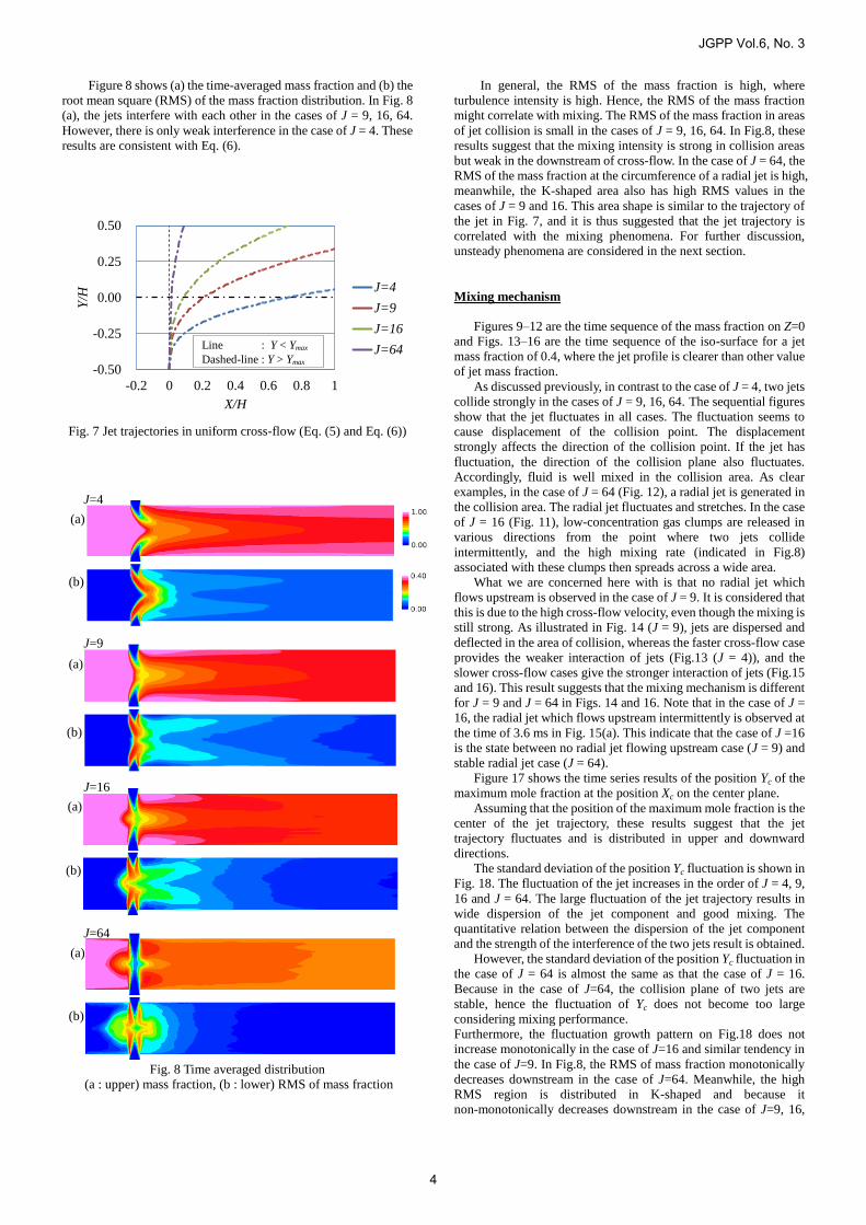
Figure 8 shows (a) the time-averaged mass fraction and (b) the

root mean square (RMS) of the mass fraction distribution. In Fig. 8

(a), the jets interfere with each other in the cases of J = 9, 16, 64.

However, there is only weak interference in the case of J = 4. These

results are consistent with Eq. (6).

-0.50

-0.25

0.00

0.25

0.50

-0.2 0 0.2 0.4 0.6 0.8 1

Y/H

X/H

J=4

J=9

J=16

J=64

Fig. 7 Jet trajectories in uniform cross-flow (Eq. (5) and Eq. (6))

Fig. 8 Time averaged distribution

(a : upper) mass fraction, (b : lower) RMS of mass fraction

In general, the RMS of the mass fraction is high, where

turbulence intensity is high. Hence, the RMS of the mass fraction

might correlate with mixing. The RMS of the mass fraction in areas

of jet collision is small in the cases of J = 9, 16, 64. In Fig.8, these

results suggest that the mixing intensity is strong in collision areas

but weak in the downstream of cross-flow. In the case of J = 64, the

RMS of the mass fraction at the circumference of a radial jet is high,

meanwhile, the K-shaped area also has high RMS values in the

cases of J = 9 and 16. This area shape is similar to the trajectory of

the jet in Fig. 7, and it is thus suggested that the jet trajectory is

correlated with the mixing phenomena. For further discussion,

unsteady phenomena are considered in the next section.

Mixing mechanism

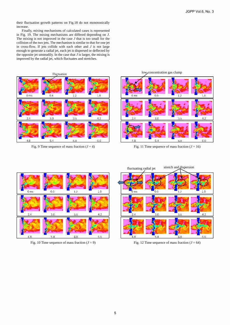
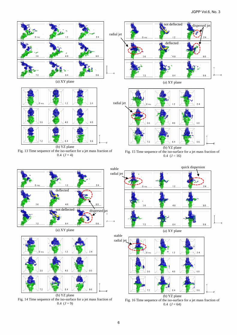
Figures 9–12 are the time sequence of the mass fraction on Z=0

and Figs. 13–16 are the time sequence of the iso-surface for a jet

mass fraction of 0.4, where the jet profile is clearer than other value

of jet mass fraction.

As discussed previously, in contrast to the case of J = 4, two jets

collide strongly in the cases of J = 9, 16, 64. The sequential figures

show that the jet fluctuates in all cases. The fluctuation seems to

cause displacement of the collision point. The displacement

strongly affects the direction of the collision point. If the jet has

fluctuation, the direction of the collision plane also fluctuates.

Accordingly, fluid is well mixed in the collision area. As clear

examples, in the case of J = 64 (Fig. 12), a radial jet is generated in

the collision area. The radial jet fluctuates and stretches. In the case

of J = 16 (Fig. 11), low-concentration gas clumps are released in

various directions from the point where two jets collide

intermittently, and the high mixing rate (indicated in Fig.8)

associated with these clumps then spreads across a wide area.

What we are concerned here with is that no radial jet which

flows upstream is observed in the case of J = 9. It is considered that

this is due to the high cross-flow velocity, even though the mixing is

still strong. As illustrated in Fig. 14 (J = 9), jets are dispersed and

deflected in the area of collision, whereas the faster cross-flow case

provides the weaker interaction of jets (Fig.13 (J = 4)), and the

slower cross-flow cases give the stronger interaction of jets (Fig.15

and 16). This result suggests that the mixing mechanism is different

for J = 9 and J = 64 in Figs. 14 and 16. Note that in the case of J =

16, the radial jet which flows upstream intermittently is observed at

the time of 3.6 ms in Fig. 15(a). This indicate that the case of J =16

is the state between no radial jet flowing upstream case (J = 9) and

stable radial jet case (J = 64).

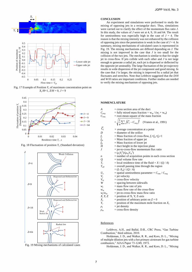
Figure 17 shows the time series results of the position Yc of the

maximum mole fraction at the position Xc on the center plane.

Assuming that the position of the maximum mole fraction is the

center of the jet trajectory, these results suggest that the jet

trajectory fluctuates and is distributed in upper and downward

directions.

The standard deviation of the position Yc fluctuation is shown in

Fig. 18. The fluctuation of the jet increases in the order of J = 4, 9,

16 and J = 64. The large fluctuation of the jet trajectory results in

wide dispersion of the jet component and good mixing. The

quantitative relation between the dispersion of the jet component

and the strength of the interference of the two jets result is obtained.

However, the standard deviation of the position Yc fluctuation in

the case of J = 64 is almost the same as that the case of J = 16. Because in the case of J=64, the collision plane of two jets are

stable, hence the fluctuation of Yc does not become too large

considering mixing performance.

Furthermore, the fluctuation growth pattern on Fig.18 does not

increase monotonically in the case of J=16 and similar tendency in

the case of J=9. In Fig.8, the RMS of mass fraction monotonically

decreases downstream in the case of J=64. Meanwhile, the high

RMS region is distributed in K-shaped and because it

non-monotonically decreases downstream in the case of J=9, 16,

Line : Y < Ymax

Dashed-line : Y > Ymax

(a)

(b)

(a)

(b)

(a)

(b)

(a)

(b)

J=4

J=9

J=16

J=64

JGPP Vol.6, No. 3

4

their fluctuation growth patterns on Fig.18 do not monotonically

increase.

Finally, mixing mechanisms of calculated cases is represented

in Fig. 19. The mixing mechanisms are differed depending on J.

The mixing is not improved in the case J that is too small for the

collision of the two jets. The mechanism is similar to that for one jet

in cross-flow. If jets collide with each other and J is not large

enough to generate a radial jet, each jet is dispersed or deflected by

the opposite jet unsteadily. In the case that J is larger, the mixing is

improved by the radial jet, which fluctuates and stretches.

Fig. 9 Time sequence of mass fraction (J = 4)

Fig. 10 Time sequence of mass fraction (J = 9)

Fig. 11 Time sequence of mass fraction (J = 16)

Fig. 12 Time sequence of mass fraction (J = 64)

low-concentration gas clump Fluctuation

interval

fluctuating radial jet stretch and dispersion

JGPP Vol.6, No. 3

5

(a) XY plane

(b) YZ plane

Fig. 13 Time sequence of the iso-surface for a jet mass fraction of

0.4 (J = 4)

(a) XY plane

(b) YZ plane

Fig. 14 Time sequence of the iso-surface for a jet mass fraction of

0.4 (J = 9)

(a) XY plane

(b) YZ plane

Fig. 15 Time sequence of the iso-surface for a jet mass fraction of

0.4 (J = 16)

(a) XY plane

(b) YZ plane

Fig. 16 Time sequence of the iso-surface for a jet mass fraction of

0.4 (J = 64)

radial jet

stable

radial jet

dispersed jet

deflected

quick dispersion

dispersed jet

deflected

stable

radial jet

not deflected

not deflected

radial jet

JGPP Vol.6, No. 3

6

-0.5

-0.4

-0.3

-0.2

-0.1

0.0

0.1

0.2

0.3

0.4

0.5

0 0.05 0.1 0.15 0.2 0.25

Po

siti

on

of

max

imu

m

con

cen

trat

ion

po

int

Yc /

H

Flow time t / Tall

Lower side jet

Upper side jet

Fig. 17 Example of Position Yc of maximum concentration point on

Xc/H=1, Z/H = 0, J = 9

0

0.05

0.1

0.15

0.2

0.25

0.3

0.35

0.4

0.45

0 0.01 0.02 0.03 0.04

Flu

ctu

atio

n o

f p

osi

tio

n Y

c

(Sta

nd

ard

dev

iati

on)

Residence time Tr , s

J = 4

J = 9

J = 16

J = 64

Fig. 18 Fluctuation of position Yc (Standard deviation)

J=4

J=9

J=64

Radial Jet

J=16

Dispersed and Deflected Jet

Weak Collision J

Weak

Radial Jet

Dispersed and Deflected Jet

Fig. 19 Mixing mechanisms of calculated cases

CONCLUSION

An experiment and simulations were performed to study the

mixing of opposing jets in a rectangular duct. Thus, simulations

were carried out to clarify the effect of the momentum flux ratio J.

In this study, the values of J were set at 4, 9, 16 and 64. The result

for unmixedness was especially high in the case of J = 4. The

reason is that the mixing intensity was not enhanced by the collision

of opposing jets since the penetration is weak in the case of J = 4. In

summary, mixing mechanisms of calculated cases is represented in

Fig. 19. The mixing mechanisms are differed depending on J. The

mixing is not improved in the case that J is too small for the

collision of the two jets. The mechanism is similar to that for single

jet in cross-flow. If jets collide with each other and J is not large

enough to generate a radial jet, each jet is dispersed or deflected by

the opposite jet unsteadily. The large fluctuation of the jet trajectory

results in wide dispersion of the jet component and good mixing. In

the case that J is larger, the mixing is improved by a radial jet that

fluctuates and stretches. Note that Lefebvre suggested that the D/H

and W/H ratios are important conditions. Further studies are needed

to verify the mixing mechanism of opposing jets.

NOMENCLATURE

A = cross section area of the duct

Cavg = fully mixed mass fraction = wm / (wj + wm)

Crms = root-mean-square of the mass fraction

=

n

i avgi CCn 1

21 (Vranos et al., 1991)

𝐶𝑖� = average concentration at a point

D = diameter of the orifice

fc = Mass fraction of cross-flow, fc+fju+fjl=1

fju = Mass fraction of upper jet

fjl = Mass fraction of lower jet

H = duct height in the injection plane

J = jet-to-cross-flow momentum flux ratio

= (ρjVj2)/(ρmVm

2)

n = number of acquisition points in each cross section

Q = total volume flow rate

Tr = local residence time of the fluid = X / (Q / A)

Tall = overall passing time through the region

= (L-XA) / (Q / A)

Us = spatial unmixedness parameter = Crms / Cavg

Vj = jet velocity

Vm = cross-flow velocity

W = spacing between sidewalls

wj = mass flow rate of jets

wm = mass flow rate of the cross-flow

wj/wm = jet-to-cross-flow mass flow ratio

X, Y, Z = position of X, Y, Z-axis

Xc = position of arbitrary point on Z = 0

Yc = position of the maximum mole fraction on Xc

ρj = jet density

ρm = cross-flow density

References

Lefebvre, A.H., and Ballal, D.R., CRC Press, “Gas Turbine

Combustion,” third edition, 2010.

Holdeman, J. D., and Walker, R. R., and Kors, D. L., “Mixing

of multiple dilution jets with a hot primary airstream for gas turbine

combustors,” AIAA Paper 73-1249, 1973.

Holdeman, J. D., and Walker, R. R., and Kors, D. L., “Mixing

Xc

Yc

JGPP Vol.6, No. 3

7

of a row of jets with a confined crossflow,” AIAA Journal, vol. 15,

no. 2, pp. 243–9, 1977.

Ogawa, N., Maki, H., Hijikata, K., “Studies on opposed

turbulent jets – impact position and turbulent component in jet

center”, JSME International Journal, Series II, vol. 35, no.2, May

1992, p.205-211

Yamamoto, K., Nomoto, A., Kawashima, T. and Nakatsuchi,

Y., “Oscillatory phenomena in coaxial impingement of opposing

jets”, J. of the Japan Hydraulics and Pneumatics Society, Vol.6,

No.2, PAGE.68-77, 1975

Andreopoulos, J., “On the structure of jets in a crossflow,”

Journal of Fluid Mechanics, vol. 157, pp. 163-197, 1985.

Fric, T.F. and Roshko, A., “Vortical structure in the wake of a

transverse jet,” Journal of Fluid Mechanics, vol. 279, pp. 1-47,

1994.

Smirnov, R. , Shi, S. and Celik., I. “Random flow generation

technique for large eddy simulations and particle-dynamics

modeling”, Journal of Fluids Engineering, 123:359-371, 2001

Lilly, D.K., “A proposed modification of the Germano

subgrid-scale closure model,” Physics of Fluids, vol. 4, pp. 633-635,

1992.

Nagao, T., and Matsuno, S., Hayashi, A.K., “Fluid Mixing of

Opposed Jet Flows in the rectangular duct”, Proceedings of 51st

AIAA Aerospace Sciences Meeting, 2012

Pitsch, H. and Steiner, H., “Scalar mixing and dissipation rate

in large-eddy simulation of non-premised turbulent combustion”,

Proceedings of the Combustion Institute, Volume 28,

2000/pp.41-49

Girimani, S. S.,and Zhou, Y. , “Analysis and modeling of

subgrid scalar mixing using numerical data”, Phys. Fluids A

8:1224-1236(1996)

Vranos, A., Lincinsky, D.S., True, B., and Holdeman, J.D.,

“Experimental study of cross-stream mixing in a cylindrical duct,”

NASA Technical Memorandum 105180, AIAA-91-2459, 1991.

JGPP Vol.6, No. 3

8