University of Tennessee, Knoxville University of Tennessee, Knoxville

TRACE: Tennessee Research and Creative TRACE: Tennessee Research and Creative

Exchange Exchange

Masters Theses Graduate School

12-2013

Effect of Disjoining Pressure and Working Fluid on Multi-Scale Effect of Disjoining Pressure and Working Fluid on Multi-Scale

Modeling for Evaporative Liquid Metal Capillary Modeling for Evaporative Liquid Metal Capillary

Hunju Yi University of Tennessee - Knoxville, hunjuyi@utk.edu

Follow this and additional works at: https://trace.tennessee.edu/utk_gradthes

Recommended Citation Recommended Citation Yi, Hunju, "Effect of Disjoining Pressure and Working Fluid on Multi-Scale Modeling for Evaporative Liquid Metal Capillary. " Master's Thesis, University of Tennessee, 2013. https://trace.tennessee.edu/utk_gradthes/2651

This Thesis is brought to you for free and open access by the Graduate School at TRACE: Tennessee Research and Creative Exchange. It has been accepted for inclusion in Masters Theses by an authorized administrator of TRACE: Tennessee Research and Creative Exchange. For more information, please contact trace@utk.edu.

To the Graduate Council:

I am submitting herewith a thesis written by Hunju Yi entitled "Effect of Disjoining Pressure and

Working Fluid on Multi-Scale Modeling for Evaporative Liquid Metal Capillary." I have examined

the final electronic copy of this thesis for form and content and recommend that it be accepted

in partial fulfillment of the requirements for the degree of Master of Science, with a major in

Mechanical Engineering.

Kenneth D. Kihm, Major Professor

We have read this thesis and recommend its acceptance:

Andreas Koschan, Kivanc Ekici, David Pratt

Accepted for the Council:

Carolyn R. Hodges

Vice Provost and Dean of the Graduate School

(Original signatures are on file with official student records.)

Effect of Disjoining Pressure and Working Fluid on Multi-Scale Modeling for Evaporative Liquid Metal Capillary

A Thesis Presented for the Master of Science

Degree The University of Tennessee, Knoxville

Hunju Yi December 2013

ii

Abstract

This research presents a new multiscale model of an evaporating liquid metal capillary meniscus under nonequilibrium evaporation sustaining a nonisothermal interface.

The primary investigation is elaborated on to examine the critical role of the disjoining pressure, which consists of both the traditional van der Waals component and a new electronic pressure component, for the case of liquid metals. The fully extended dispersion force is modeled along with an electronic disjoining pressure component that is unique to liquid metals attributing to their abundant free electrons. For liquid alkali metals (sodium and lithium), as a favorable coolant for high temperature two-phase devices, the extended meniscus thin film model (sub-microscale) is coupled to a CFD model of the evaporating bulk meniscus (sub-millimeter scale).

Two extreme cases of sodium are compared, i.e. with or without incorporation of the electronic disjoining pressure component. It is shown that the existence of electronic component of the disjoining pressure leads towards larger total capillary meniscus surface areas and larger net evaporative mass flow rates. Furthermore, the net evaporative mass flux in the bulk meniscus region is needed to accounted for to obtain a true picture of the total capillary evaporation transport.

Comparative study of sodium(Na) and lithium(Li) coolants with existence of the electronic disjoining pressure is performed. The heat pipe with lithium coolant shows enhanced thin film area and higher heat transfer capability with less evaporative mass flux than one with sodium coolant does under the same overheating condition.

iii

Table of Contents

Chapter 1 Introduction and Background ............................................................................. 1

Introduction ..................................................................................................................... 1 Backround ....................................................................................................................... 3

Chapter 2 Modeling Evaporative Thin Film ...................................................................... 8 2.1 Complex Dielectric Permittivity ............................................................................. 12 2.2 Fermi Energy and work funcion ............................................................................. 18 2.3 Numerical Analysis Techniques ............................................................................. 22

Chapter 3 Modeling Bulk Meniscus ................................................................................ 24 Chapter 4 Bulk Meniscus and Thin Film Interface Boundary Conditions ...................... 27 Chapter 5 Results and Discussion .................................................................................... 29

5.1 Comparative study of different disjoining pressures for sodium ............................ 29 5.2 Comparative study of sodium and lithium coolant ................................................. 38

Chapter 6 Results and Discussion .................................................................................... 45 List of References ............................................................................................................. 47 Vita .................................................................................................................................... 51

iv

List of Tables

Table 1. Fluidic and thermodynamic properties of liquid sodium at atmospheric pressure..................................................................................................................................... 15

Table 2. Two variations in the boundary condition term of Derjaguin’s electronic component of the disjoining pressure and its effect on the adsorbed film thickness as well as the scaling of the nondimensionalized liquid metal thin film equation. ....... 30

Table 3. Fluidic and thermodynamic properties of liquid sodium and lithium at atmospheric pressure. ................................................................................................ 40

v

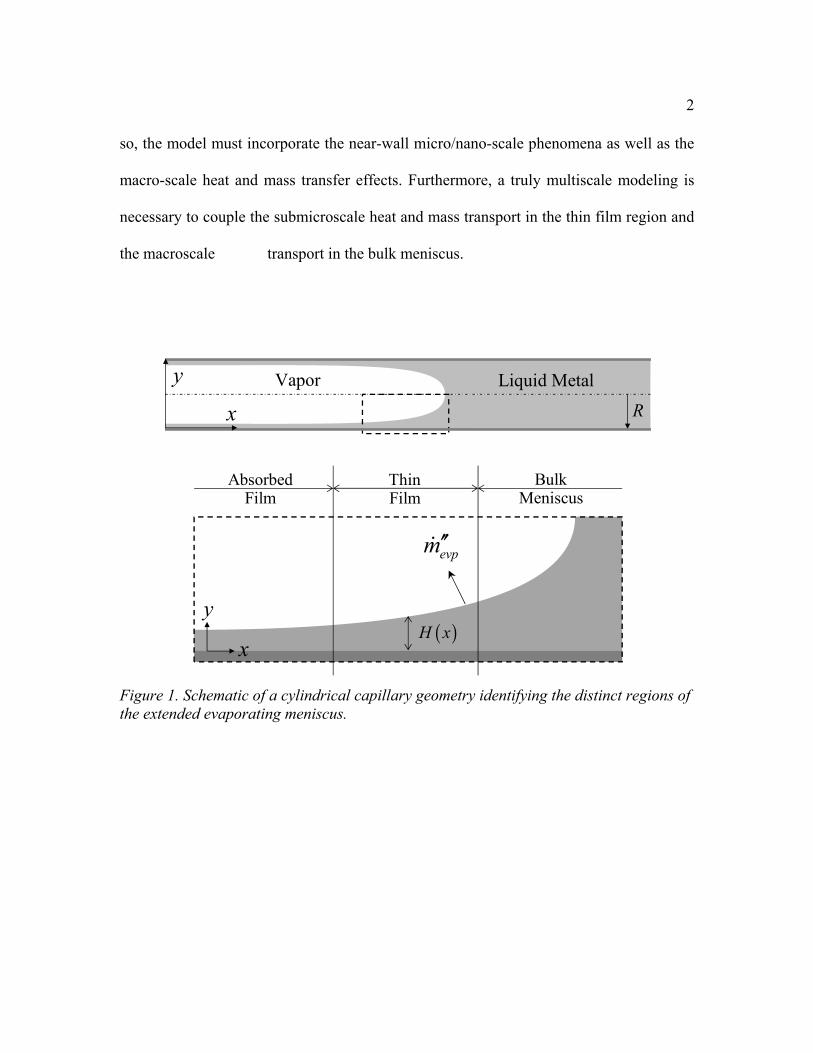
List of Figures Figure 1. Schematic of a cylindrical capillary geometry identifying the distinct regions of

the extended evaporating meniscus. ........................................................................... 2 Figure 2. Experimentally determined temperature-dependence of the work function of

sodium, and experimentally extrapolated Work Function versus the Fermi Energy ................................................................................................................................... 20

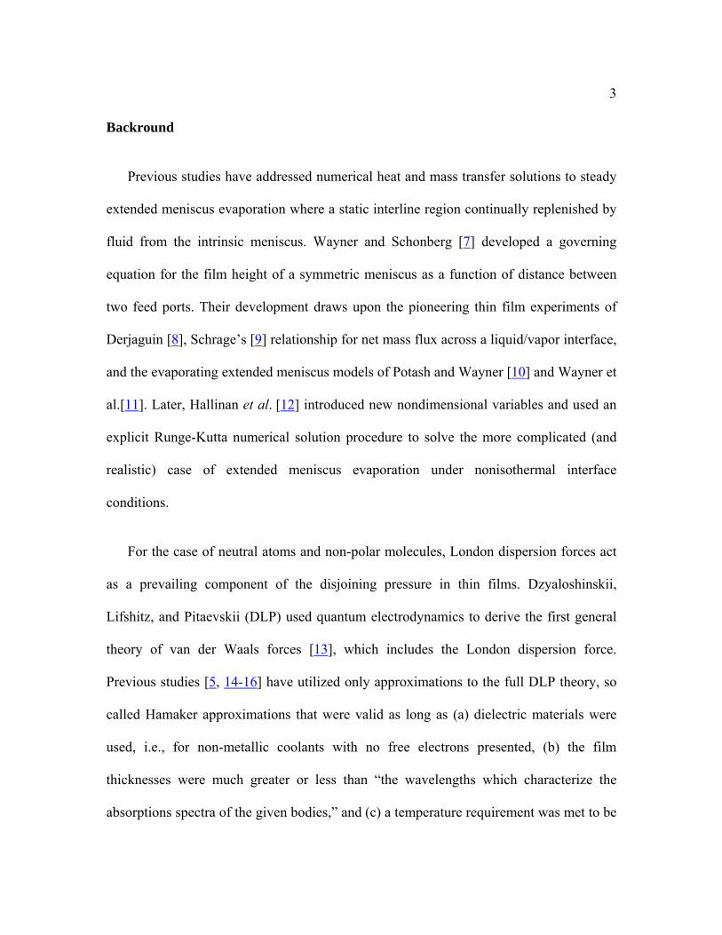
Figure 3. A schematic of the bulk evaporating capillary meniscus CFD geometry and boundary conditios, and meshes generated by COMSOL ........................................ 25

Figure 4. Steady total capillary meniscus evaporation solutions of sodium ..................... 32 Figure 5. COMSOL CFD model of an evaporating sodium capillary meniscus .............. 33 Figure 6. Column bar charts which compare the extended meniscus thin film and bulk

meniscus contributions to capillary meniscus surface area and net evaporative mass flow rate. ................................................................................................................... 37

Figure 7. Temperature-dependence of the Fermi Energy and Work Function of lithium. 41 Figure 8. Steady total capillary meniscus evaporation solutions of sodium and lithium . 43 Figure 9. Column bar charts which compare the extended meniscus thin film and bulk

meniscus contributions to capillary meniscus surface area and net evaporative mass flow rate. ................................................................................................................... 44

vi

List of Symbols a1,2,3 thin film boundary conditions A Hamaker constant [J] B disjoining pressure electronic component constant [N] Ca capillary number [Ca = μlu0⁄γ] cP specific heat capacity at constant pressure [J⁄kg] hfg latent heat of evaporation [J⁄kg] H film thickness [m] H0 adsorbed film thickness [m] ħ Reduced Planck constant (Dirac’s constant) [J / s] i imaginary number [√−1] K thin film curvature [m-1] me electron mass [kg] m"

evaporative mass flux [kg⁄s · m2] M molar mass [kg⁄mol] Ne valence electron number density [m-3] P pressure [N⁄m2] qe electron charge [C] q′′ heat flux [W⁄m2] r radial coordinate (cylindrical CS) [m] R pore radius [m]

R universal gas constant [N · m⁄K · mol] S surface domain of integration SA surface area [m2] T temperature [K] T* nondimensional interfacial temperature ΔT liquid overheat [K] u horizontal velocity [m⁄s] v vertical velocity [m⁄s] ve plasma frequency of an electron gas [Hz] x axial coordinate (Cartesian CS) [m] y vertical coordinate (Cartesian CS) [m] z horizontal coordinate (cylindrical CS) [m] Greek Symbols α evaporation coefficient γ surface tension [N⁄m] ɛ0 Permittivity of free space [ ∙ / ∙ ] ɛ1 relative permittivity of container ɛ2 relative permittivity of vapor ɛ3 relative permittivity of liquid thin film η nondimensional axial coordinate [η = x⁄x0]

vii

θ radial coordinate (cylindrical CS) [rad] θ nondimensional film thickness [θ(η) = H⁄H0] κ ratio of evaporative interfacial resistance to conductive resistance κn electronic disjoining pressure work function parameter λ thermal conductivity [W/m·K] μ viscosity[N·s/m2] Π disjoining pressure [N⁄m2] Π nondimensional disjoining pressure [Π = Π/Π ] ρ density [kg⁄m3] σ optical conductivity [S⁄m] τ relaxation time [s] χ electronic disjoining pressure boundary condition ω frequency [rad⁄s] ωe plasma frequency of an electron gas [rad⁄s] ωn electromagnetic wave frequency [rad⁄s] Subscripts 0 reference state A dispersion component of the disjoining pressure B electronic component of the disjoining pressure lv liquid/vapor interface l liquid tf thin film v vapor w wall

1

Chapter 1

Introduction and Background

Introduction

Effective cooling schemes for high power density electronics, space-based nuclear

reactors, hypersonic vehicle leading edges, and the like share a need for high temperature

coolant operation and mass minimization. Liquid metal heat transport devices, such as

heat pipes and capillary pumped loops, have the potential to meet these needs [1-4]. Their

evaporative capacity and stability, however, depends upon accurate modeling of the

evaporating extended meniscus region [5]. The interline or contact line region of an

evaporating extended meniscus consists of three subregions in multiscales as

schematically shown in Figure 1: the adsorbed region where a disjoining pressure

dominates the local atomic forces; the intrinsic or bulk meniscus region where the

interfacial curvature governs the driving physics through surface tension; and the

transition or thin-film region in between where both the disjoining pressure and the

interfacial curvature share a comparable influence. Liquid alkali metals, such as sodium

and lithium, present complexities in the disjoining pressure models that have received

little attention in the literature. In contrast to ordinary coolants such as water or pentane,

the presence of abundant free electrons in liquid metals necessitates the additional

“electronic pressure” or “electron degeneracy” contributions to the disjoining pressure [6].

This study seeks to address these modeling issues associated with liquid metal in the

context of a physically realistic nonisothermal model of the evaporating thin film. To do

2

so, the model must incorporate the near-wall micro/nano-scale phenomena as well as the

macro-scale heat and mass transfer effects. Furthermore, a truly multiscale modeling is

necessary to couple the submicroscale heat and mass transport in the thin film region and

the macroscale transport in the bulk meniscus.

Figure 1. Schematic of a cylindrical capillary geometry identifying the distinct regions of the extended evaporating meniscus.

evpm′′

( )H x

Vapor Liquid Metal

Rx

y

AbsorbedFilm

ThinFilm

BulkMeniscus

y

x

3

Backround

Previous studies have addressed numerical heat and mass transfer solutions to steady

extended meniscus evaporation where a static interline region continually replenished by

fluid from the intrinsic meniscus. Wayner and Schonberg [7] developed a governing

equation for the film height of a symmetric meniscus as a function of distance between

two feed ports. Their development draws upon the pioneering thin film experiments of

Derjaguin [8], Schrage’s [9] relationship for net mass flux across a liquid/vapor interface,

and the evaporating extended meniscus models of Potash and Wayner [10] and Wayner et

al.[11]. Later, Hallinan et al. [12] introduced new nondimensional variables and used an

explicit Runge-Kutta numerical solution procedure to solve the more complicated (and

realistic) case of extended meniscus evaporation under nonisothermal interface

conditions.

For the case of neutral atoms and non-polar molecules, London dispersion forces act

as a prevailing component of the disjoining pressure in thin films. Dzyaloshinskii,

Lifshitz, and Pitaevskii (DLP) used quantum electrodynamics to derive the first general

theory of van der Waals forces [13], which includes the London dispersion force.

Previous studies [5, 14-16] have utilized only approximations to the full DLP theory, so

called Hamaker approximations that were valid as long as (a) dielectric materials were

used, i.e., for non-metallic coolants with no free electrons presented, (b) the film

thicknesses were much greater or less than “the wavelengths which characterize the

absorptions spectra of the given bodies,” and (c) a temperature requirement was met to be

4

in a moderate range [13]. The case of a high temperature, liquid metal, evaporating thin

film, however, invalidates each of these assumptions.

Furthermore, the founder of the disjoining pressure concept proposed the existence of

an additional form of disjoining pressure unique to liquid metal films [6, 17]. Derjaguin

and coworkers surmised that the free electrons in a thin metal film, modeled as a fermion

gas, would experience a confinement in their position. This electron degeneracy creates

an increase of the energy density in the thin film, according to Heisenberg’s uncertainty

principle, and produces an effective “electron pressure” (for a good summary, see

Roldughin [18]). Derjaguin et al. [6] indirectly proved the existence of the electronic

component to the disjoining pressure by experiment. Derjaguin and Roldughin [18] were

able to derive a relationship between the change in kinetic energy of free electrons in the

thin film and the disjoining pressure using quantum mechanical theory. The resulting

electron degeneracy disjoining pressure varies in intensity and sign depending upon the

work function (energy needed to move an electron from the liquid metal to the solid

surface) of the system.

Using an additive model of the disjoining pressure, which was first proposed by

Ajaev and Willis [19, 20], Tipton et al. [21] successfully modeled a liquid sodium

evaporating thin film using both the retarded dispersion and electronic disjoining pressure

components. An isothermal thin film assumption was used along with a simplified model

of the dielectric constants of sodium. Results indicated that variation in the work function

can produce multiple order-of-magnitude differences in the film thickness and

5

evaporation profile. The evaporation profiles could not be integrated, however, due to the

unrealistic isothermal film assumption. In addition, it was speculated that the high

thermal conductivity of liquid sodium would necessitate a model that included

evaporation in the bulk meniscus region.

For the cases of non-metallic coolants, several authors have attempted to model the full

capillary evaporating meniscus at steady-state with varying degrees of complexity and

success. Swanson and Herdt [22] attempted to model the entire micro- and macro-

capillary domain using one characteristic set of equations. Interestingly, Chebaro et

al. [23] pointed out that “Swanson and Herdt’s analysis inexactly made assumptions

pertaining to the curvature of the interface in the interline region, the radial pressure

gradient in the meniscus, and the tangential shear stress boundary condition at the

interface in the meniscus.”

Stephan and Busse [24] sought to model a grooved heat pipe wall geometry. Their thin

film extended meniscus model only included an isothermal interface and thermocapillary

forces were assumed negligible. The wall temperature in the micro region was assumed

specified and the thin film solution yielded the curvature of the bulk meniscus, the

temperature distribution at the interface, and the total heat transferred into the micro

region. Heat transfer in the bulk meniscus fluid region and groove walls was solved via a

FEM conduction model that did not consider fluid flow. The capillary surface was

considered static and nonevaporative. The micro and macro region models were iterated

until they agreed on the wall temperature and heat flux at their interface.

6

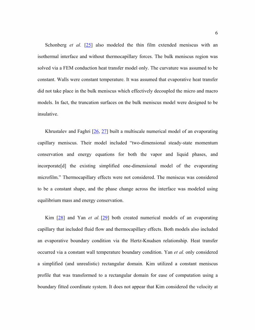
Schonberg et al. [25] also modeled the thin film extended meniscus with an

isothermal interface and without thermocapillary forces. The bulk meniscus region was

solved via a FEM conduction heat transfer model only. The curvature was assumed to be

constant. Walls were constant temperature. It was assumed that evaporative heat transfer

did not take place in the bulk meniscus which effectively decoupled the micro and macro

models. In fact, the truncation surfaces on the bulk meniscus model were designed to be

insulative.

Khrustalev and Faghri [26, 27] built a multiscale numerical model of an evaporating

capillary meniscus. Their model included “two-dimensional steady-state momentum

conservation and energy equations for both the vapor and liquid phases, and

incorporate[d] the existing simplified one-dimensional model of the evaporating

microfilm.” Thermocapillary effects were not considered. The meniscus was considered

to be a constant shape, and the phase change across the interface was modeled using

equilibrium mass and energy conservation.

Kim [28] and Yan et al. [29] both created numerical models of an evaporating

capillary that included fluid flow and thermocapillary effects. Both models also included

an evaporative boundary condition via the Hertz-Knudsen relationship. Heat transfer

occurred via a constant wall temperature boundary condition. Yan et al. only considered

a simplified (and unrealistic) rectangular domain. Kim utilized a constant meniscus

profile that was transformed to a rectangular domain for ease of computation using a

boundary fitted coordinate system. It does not appear that Kim considered the velocity at

7

the evaporative surface to be specified through the evaporative mass flux. Neither study

considered the effects of thin film extended meniscus evaporation in the micro region.

Despite the long history of characterizing thin film evaporative non-metal coolants,

study of fundamental physics of evaporating metallic coolants has been scarce to date.

This work presents a new multiscale and comprehensive model of an evaporating liquid

metal capillary meniscus, including the thin film region as well as the bulk region, with a

nonisothermal interface while under nonequilibrium evaporation. In particular,

elaboration has been made to systematically examine the critical role of the disjoining

pressure, which consists of both the traditional van der Waals component and a new

electronic pressure component, for the case of liquid metals.

8

Chapter 2

Modeling Evaporative Thin Film

Tipton et al. [21] utilized the thin film equations of Chebaro and Hallinan [30] and

Chebaro et al. [23] for the case of an isothermal liquid/vapor interface. The present work

utilizes the thin film equations of Hallinan et al. [12] for a nonisothermal and more

realistic liquid/vapor interface. The following dimensionless variables are defined as:

θ = H

H0

, η = x

x0

, ∏ = ∏∏

0

, Ca =μlu0

γ, x0 =

γ H0

∏0

′′m0 = ρlu0 = 2α2 − α

Μ2πR Tv

1/2PvM hfg

R TvTlv

Tw − Tv( )

∏0

=M h

fgΔT

VlT

v

, ΔT0

= Tw

− Tv

The governing equation for the evaporating thin film then becomes

( ) ( ) ( ) ( ) ( ) ( ) [ )3 3 *2

0 0

* * , 0,3Ca

TH

θ η θ η θ η θ θ η θ η

γ

′ − ′′′ ′ ′′+ = − −

Π

Π ∈ ∞Π

(1)

where the boundary conditions are given:

( ) 10 aθ = (1a)

( ) 20 aθ ′ = (1b)

9

( ) 3aθ ′′ ∞ = (1c)

( )0 0θ ′′′ = (1d)

The initial perturbations of the dependent variable θ and its first derivative are

necessary to avoid a trivial solution and do correspond to physical realities as described

in Hallinan et al. [12] where a1 = 1.030 and a2 = 0.0004. The boundary condition on the

second derivative of the dependent variable is a3 = K where K is the curvature of the bulk

meniscus region. Thus, in practice, η = ∞ is taken to be a point in the far field, lmax, where

the second derivative approaches an asymptotic value that is the reciprocal of the pore

radius K = 1⁄R.

The main difference between the isothermal and nonisothermal interface governing

equations lies with the inclusion of a nondimensional interfacial temperature term, T*, in

Eq. (1):

( ) ( ) ( )

( )0

*

0

lv v

w v

TT T

TT T T

κθ η θ η θ

κθ η

′′Δ + + ∏ − = =− Δ +

(2a)

where κ , the ratio of evaporative interfacial resistance to conductive resistance, is

( )0

0/fgh m

Hκ

λ′′

=

(2b)

10

which then modifies the net evaporative mass flux to

( ) ( )*0evpm m T θ η θ ′′′′ ′′= − − ∏

(3)

The liquid pressure gradient of isothermal interface remains unchanged for nonisothermal

interface as:

( ) ( )0

0

dP

dx xθ η θ∏ ′′′ ′= − +∏

(4)

An accurate disjoining pressure model for liquid metals is of the form [21]:

( ) ( ) ( ) [ ],1

0 0

, , , 1,2, ,75A i Bi i i

θ θθ θ θ θ +

∏ ∏∏ = + = =

∏ ∏ (5)

The expanded van der Waals contribution (ΠA) is given in terms of the macroscopic

dielectric permittivity, ε , from consideration of the full DLP theory [13] as:

( ) ( )( )( )( )

( )( )( )( )

1

1 23/2 3 23 33 1

0 1 2

1

1 1 3 2 2 33

1 1 3 2 2 3

2exp 1

/ / 2exp 1

/ /

nA n p

n

n

s p s p p HkTH p

c s p s p c

s p s p p Hdp

s p s p c

ωε ω επ

ε ε ε ε ω εε ε ε ε

−∞ ∞

==

−

+ + − ∏ = − − − + + + − − −

(6a)

where

211

3

1s pεε

= − + (6b)

11

222

3

1s pεε

= − + (6c)

2

n

nkTπω =

(6d)

( )niε ε ω= (6e)

with the subscripts 1, 2 and 3 referring to substrate, vapor, and liquid metal, respectively.

The fully retarded dispersion force component ΠA is modeled using a 75 piece cubic

spline interpolation.

The electronic component ΠB depends upon a work function boundary condition. The

free electrons in a thin metal film will experience a confinement in their positions and

this electron degeneracy creates an increase of the energy density and produces an

effective “electron pressure”. Therefore, an additional contribution to the disjoining

pressure needs to be accounted for in the liquid metal thin film as [17];

( ) ( )

2

2;

2e

B n

NBH B

H m Vχ κΠ ≈ =

(7a)

The parameter κn is itself closely related to the work function, W: the energy needed to

move an electron from the liquid metal to the solid surface [21]

( ) 2

1 2 1

1

4nχ κ = Σ Σ − Σ

(7b)

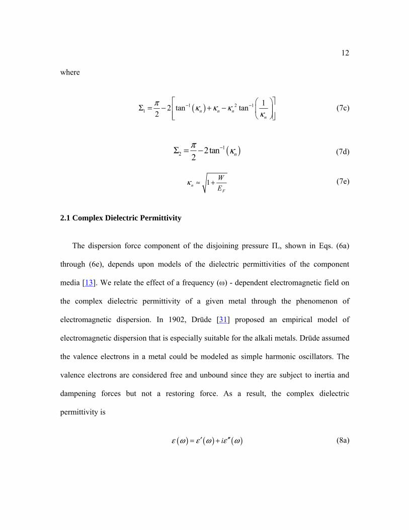
12

where

( )1 2 11

12 tan tan

2 n n nn

π κ κ κκ

− − Σ = − + −

(7c)

( )12 2tan

2 n

π κ−Σ = − (7d)

1nF

W

Eκ ≈ + (7e)

2.1 Complex Dielectric Permittivity

The dispersion force component of the disjoining pressure ΠA, shown in Eqs. (6a)

through (6e), depends upon models of the dielectric permittivities of the component

media [13]. We relate the effect of a frequency (ω) - dependent electromagnetic field on

the complex dielectric permittivity of a given metal through the phenomenon of

electromagnetic dispersion. In 1902, Drüde [31] proposed an empirical model of

electromagnetic dispersion that is especially suitable for the alkali metals. Drüde assumed

the valence electrons in a metal could be modeled as simple harmonic oscillators. The

valence electrons are considered free and unbound since they are subject to inertia and

dampening forces but not a restoring force. As a result, the complex dielectric

permittivity is

( ) ( ) ( )iε ω ε ω ε ω′ ′′= + (8a)

13

( )2 2

2 21

1eω τε ωω τ

′ = −+

(8b)

( ) ( )2

2 21eω τε ω

ω ω τ′′ =

+ (8c)

where τ represents the relaxation time, which is related to the DC conductivity via the

Lorentz-Sommerfeld relation [32]

20 /e e em N qτ σ= (8d)

and ωe symbolizes the plasma frequency of the free electron gas

20/e e e eN q mω ε= (8e)

Hodgson [33] provides a detailed derivation and explanation of the pertinent

simplifying assumptions. Above all, it should be noted that this development ignores the

magnetic permeability (μ/μo ~ 1.0) in accordance with Maxwell’s relation, i.e., ɛ(ω) ≈

n2(ω). Inagaki et al. [34] found good correlation between the Drüde Theory and

experimental results for liquid Sodium at 120ºC at lower frequencies of excitation. The

discrepancy at higher frequencies arises from the assumption that the dielectric

permittivity is independent of the wave number of the incoming electromagnetic wave

[35]. It is not modeled in this case for the sake of simplicity.

In reality, electrons experience influence from the positive ions in the metal as well as

other electrons. The electron mass, me, or free electron density, Ne, are multiplied by an

14

empirical “fudge factor” in an effort to accommodate these influences and make this

extremely simplified model more closely resemble experimental data. The presence of a

superscript * indicates the use of an effective value. For liquid Sodium, Shimoji [36]

reported an effective valence electron number density of Ne*⁄N e = 0.85 at 1000C. Inagaki

et al. [34] reported an effective mass me*⁄m e = 1.17 at 1200C. These empirical terms are

essentially equivalent since Ne*⁄N e = me ⁄me

*. In the absence of any further experimental

results, we assume this value holds at the melting point of liquid sodium, as well. The

plasma frequency for liquid sodium at the melting point is calculated to be ve,3 = 1.0675 ×

1015Hz using Eq. (6e) with the effective mass and the properties listed in Table 1.

15

Table 1. Fluidic and thermodynamic properties of liquid sodium at atmospheric pressure. The evaporation coefficient of sodium was reported by Takens et al [37]. The resistivity was extrapolated from curve fits summarized by Wilson [38]. All other properties were obtained from the Argonne National Laboratory International Nuclear Safety Center Material Properties Database as reported by Fink and Leibowitz [39].

Property Symbol Units Sodium Water

Vapor Temperature Tv K 1156.1 373.12

Molecular Mass M kg⁄mol 0.02299 0.018015

Density ρ kg⁄m3 742.86 959.24

Dynamic Viscosity μ N·s/m2 1.5856E-04 2.8064E-04

Surface Tension γ N⁄m 0.1199 0.0593

Thermal Conductivity λ W/m·K 48.6562 0.6798

Latent Heat of Vaporization hfg KJ⁄kg 3881.5 2218.9

Vapor Pressure Pv MPa 0.10133 0.10133

Electrical Conductivity σ S⁄m 2.54E+06 5.5E-06

Evaporation Coefficient α 1.0 0.2 ~ 1.1

The solid substrate for the capillary wall is chosen to be ANSI type 304 stainless steel

(SS304). The simplified Drüde model is used which assumes no damping forces

( )2

1 eωε ωω

= +

(9)

where ωe is the plasma frequency of the electron gas as given in Eq. (8e). The

composition is approximated as Fe (71%), Cr (19%), Ni (9%) yielding an atomic weight

16

of 54.81 with 1.79 valence electrons per molecule and a density of 8000 kg⁄m3. These

values yield a plasma frequency for solid SS304 of ve,1 = 3.5615 × 1015Hz using Eq. (8e).

It is important to note that the DLP equation requires the three media to be modeled

in terms of their respective dielectric permittivities for imaginary frequencies. This is

related to the imaginary part of the dielectric permittivity for real frequencies through the

relationship

( ) ( )2 20

21

x xi dx

x

εε ω

π ω∞ ′′

= ++ (10)

which was derived from the Kramers-Kronig relation using contour integrals [40]. Here,

the imaginary part of the complex dielectric permittivity (ε ′′ ) “is always positive and

determines the dissipation of energy in an electromagnetic wave propagated in the

medium” [13]. For liquid sodium, substitution of Eq. (8c) into Eq. (10) yields

( ) ( )( )

2,3

3 2 2

11

1ei

ω τ ωτε ω

ω ω τ−

= +−

(11)

For the solid stainless steel substrate, Eq. (9) does not contain a complex part. Thus,

the dielectric permittivity for imaginary frequencies is

( )2

,11 1 ei

ωε ω

ω

= −

(12)

17

using the substitution of iω for ω. For the sodium vapor, the dielectric permittivity for

imaginary frequencies is simply unity (i.e. ɛ 2(iω) = 1).

18

2.2 Fermi Energy and work funcion

The electronic force component of the disjoining pressure ΠB , shown in Eqs (7a) –

(7e), depends on both the Fermi energy (EF) and work function (W) of a specific liquid

metal coolant. The Fermi energy for a metal is defined as the energy level at which the

opportunity to attract an electron is the same as the opportunity to lose it. In other words,

Fermi energy is the energy at which electrons cannot be bound to a single nucleus

because the nucleus has no more available spots for electrons. Fermi energy is outlined

by Coutts using the Fermi-Dirac distribution [41]

2 4

2 4

@ ( ) @ 0( )@ 0( ) @ 0( )

112 80

B BF T Kelvin F Kelvin

F Kelvin F Kelvin

k T k TE E

E E

π π = − −

(13)

E F @1156.1K = 3.19744 (eV)

where the Boltzmann constant is 8.61734315×10-5eV/K and the Fermi energy level at

T = 0K is @ 0F KE = 3.2 (eV).

The work function is defined as the minimum energy needed to remove an electron

from a solid to a point outside the solid’s surface, or equivalently, to move an electron

from Fermi level to vacuum level. Knowledge of the proper work function for a given

system depends heavily on a quantum mechanical description of the system that is

intimately tied to the surface conditions of the contacting medium. The work function is

kB

19

also known as a gradual function of temperature, and Alchagirov et al. [42] provides

experimentally measured work functions of sodium.

20

Figure 2(a). Experimentally determined temperature-dependence of the work function of sodium under heating (●) and cooling (○). [42], and (b) experimentally extrapolated work function (Eq. 14) versus the Fermi Energy (Eq. 13).

0

0.5

1

1.5

2

2.5

3

3.5

0 100 200 300 400 500 600 700 800 900 1000 1100

Fermi Energy Work Function

(b)

Ene

rgy

Lev

el (

eV)

Temperature (K)

2.35

2.4

2.45

2.5

100 150 200 250 300 350 400 450

Heating

CoolingmeltT

Solid Liquid

(a)

Ene

rgy

Lev

el (

eV)

Temperature (K)

21

Based on the published data (Fig. 2a), the work function of liquid sodium at its

operation temperature around the standard boiling temperature (1,156.1K) and the

equation are extrapolated as:

4( ) 2.51 (3.27 10 ) 2.132W T T−= − × = eV (at T = 1156.1K) (14)

Figure 2b shows the Fermi energy of sodium as a function of temperature (Eq. 13) as

well as the extrapolated work function (Eq. 14).

The constant part of B, as defined in Eq. (7a), is calculated at the melting point of

liquid sodium following Derjaguin’s method as ( )101.1873 10B χ κ−= × ⋅ , with the

boundary condition parameter χ varying with κ, which is itself a function of the work

function, as shown in Eq. (7e).

This expression was derived assuming a free surface on either side (e.g. a bubble thin

film). In a practical heat pipe situation, the top side would be a free surface while the

bottom side would interface with a metal-alloy substrate. Thus, this expression serves as

a first order approximation. Accordingly, we consider two extreme cases to draw

comparisons: zero work function ( 0BΠ = ) that neglects the electron degeneracy force

contributions to the disjoining function, and the maximum possible work function that

corresponds to the liquid metal-vacuum interface. For the latter case of the maximum

work function, the following calculation parameters are determined from Eqs. (7) to (9):

1.2910≈nκ

22

( ) 059464.0=nκχ

B[N ] = 7.0602E −12

0[ ] 75.277482H nm =

68.98/ =ΠΠ AB

Particular attention can be given to ΠB / ΠA depending on the electronic disjoining

pressure work function κn. Thin film profiles, evaporative mass flux distributions, and the

inner pressure gradients are determined from numerically solving Eqs. (1) to (4) for the

aforementioned two extremes of work functions, i.e., no contribution from electron

degeneracy forces ( / 0B AΠ Π = ) as well as its maximum possible contribution

( / 98.68B AΠ Π = ) with the work function specified at T = 1156.1K, the boiling point of

sodium at 1 atm. The former corresponds to the non-existence of free electrons in sodium,

while the latter corresponds to the development of a sodium thin film in the vacuum

without being contacted by any solid surfaces. In practice, the sodium thin film contacts

metal heating surfaces under evaporation and thus the corresponding work function must

be intermediate between the two extremes.

2.3 Numerical Analysis Techniques

Using a coordinate transformation from max[0, ]lη = to [ 1,1]ξ = − by letting

( ) ( )( )ˆ 1θ ξ θ φ ξ= + where max / 2lφ = , the governing equation for the evaporating thin

film, Eq. (1), is transformed to [21]:

23

( ) ( ) ( ) ( ) ( ) ( ) ( ) ( ) ( ) ( )

( ) ( ) [ ]

2 3 2 3* *4

0

*

4

*2 2

0

3 1 3ˆ ˆ ˆ ˆ ˆ ˆ ˆ ˆ ˆ ˆ

3 1 ˆ ˆ 1, ,1Ca

TH

θ ξ θ ξ θ ξ θ ξ θ ξ θ ξ θ ξ θ θ ξ θφφ φ

θ ξ θ ξφ

γ

Π Π

Π ∈ −Π

′ ′′′ ′′′ ′′′′ ′+ + +

− ′′= − −

(15)

where the corresponding B.C.s’ are given by ( ) 1ˆ 1 aθ − = , ( ) 2

ˆ 1 aθ φ′ − = , ( ) 23

ˆ 1 aθ φ′′ = ,

( )ˆ 1 0θ ′′′ − = .

Equation (15) is solved using orthogonal collocation with Chebyshev polynomials of

the first kind as the basis function. The collocation coefficients are found via the

Levenberg-Marquardt method performing an optimum interpolation between the

Newton-Raphson method and the method of steepest descent method. Also maximum

axial length ( max 2l φ= ) needs optimization to prevent results from undulating θ̂ ′′′ when

maxl is deficient and losing details with excessive maxl .

24

Chapter 3

Modeling Bulk Meniscus

This research distinguishes itself from previous works as it models multiscale liquid

metal capillary evaporation with a nonisothermal interface and nonequilibrium meniscus

evaporation. The continuity and momentum equations for the bulk domain in cylindrical

coordinates (Fig 3-a) are given as:

( ) ( )10

vru ru

r r z

∂ ∂+ =∂ ∂

(16a)

2

2 2

1u u p u u uu v r

r z r r r r z rρ μ ∂ ∂ ∂ ∂ ∂ ∂ + = − + + − ∂ ∂ ∂ ∂ ∂ ∂

(16b)

2

2

1v v p v vu v r

r z z r r r zρ μ ∂ ∂ ∂ ∂ ∂ ∂ + = − + + ∂ ∂ ∂ ∂ ∂ ∂

(16c)

for an incompressible fluid with constant density and viscosity. Buoyancy forces are

considered to be negligible for the microscale configurations at present. Assuming

constant density, specific heat, and thermal conductivity, the energy equation is given as:

2

2

1p

T T T Tc u v r

r z r r r zρ λ ∂ ∂ ∂ ∂ ∂ + = + ∂ ∂ ∂ ∂ ∂

(16d)

25

Figure 3. A schematic of the bulk evaporating capillary meniscus CFD geometry and boundary conditions, and meshes generated by COMSOL

Figure 3-a details the full problem geometry and boundary conditions. The right side

represents the capillary wall with no-slip velocity and constant temperature boundary

conditions. The left side represents the symmetry line through the center of the capillary.

As such, the slip/symmetry boundary conditions are utilized in the momentum equations,

and the energy equation boundary condition is adiabatic. The top surface represents the

outflow boundary, namely the evaporating bulk meniscus. At the surface of the

z

/evp l

N

evp fg

u n m

q n m h

ρ→

⋅ =

⋅ =

( )

0uv

T r

=

0,'

Hu T Tv Stoke s Flow

= ==

0

w

u v

T T

= ==

0

0

Nq

dvu

dr

=

= =

Men

iscu

s A

rea

Thi

n F

ilm

A

rea

r

tfH

26

evaporating bulk meniscus, the velocity and heat flux are specified as functions of surface

temperature via the Hertz-Knudsen-Schrage (HKS) relationship,

( ) ( )1/2

2

2 2v fg l v

evp lv vv v lv lv

P h V Pm T T K

T T T T

α γα π

Μ ′′ = − + −

M

R R R (17)

which describes the net evaporative mass flux under non-equilibrium conditions [43].

The bottom surface of the capillary represents the inflow boundary. Fully developed

flow is assumed, thus the velocity profile is that of Stoke’s Flow and the flow

temperature is that of the wall. The velocity profile is scaled to conserve mass according

to the specified outflow conditions along the meniscus interface to ensure that the

meniscus boundary remains static in space and time.

27

Chapter 4

Bulk Meniscus and Thin Film Interface Boundary Conditions

The interface between the bulk meniscus and thin film models must match in

thickness, mass flow, and temperature/heat flux. The thin film solution is thus used to

specify the boundary conditions for the bulk meniscus model at the interface. The

thickness requirement also affects the meniscus shape. The curvature of the meniscus z(r)

is considered constant (per previous developments) and inversely proportional to the

radius of the capillary tube, R. The bulk meniscus profile is thus given by

( )2

2

( ) , [0, ]2 2

tf

tf

R Hrz r r R H

R R

−= + ∈ − (18)

where, at the capillary center line, the meniscus slope is considered to be zero. Instead of

approaching the wall and creating a singularity condition, the bulk meniscus is ended at a

point (r = R - Htf) that matches the far field solution of the extended meniscus thin film

evaporation model presented previously. Here, Htf is the thin film height at the asymptotic

far-field boundary condition (Eq. 1-c) interpreted as H(lmax).

The mass flow boundary condition is met by establishing a uniform outflow velocity

over the thin film thickness that equals the total evaporative mass flow of the evaporating

thin film. This is achieved in Eq. (20) as:

( )22

evp evp

tf

m mv

SA R R Hρ ρπ= =

⋅ − −

(19)

28

where SA denotes the cross-sectional area of the replenishing axial flow. The total

evaporative mass flow is calculated from the thin film solution using Eq. (15):

( )2

@

0

ˆ 2 1tfx

evp Thin Film evp evp

S x

dym m ndS R m x dx

dxπ

→

=

′′ ′′= ⋅ ≈ + (20)

This boundary condition model is consistent with the assumption of lubrication theory

fluid flow that was used to construct the extended meniscus thin film model.

Finally, a 1D conduction model was assumed to model heat transfer through the

extended meniscus thin film. Thus, the interfacial temperature distribution along the

radius is given as:

( )( ) evp fgw

m hT r T R r

λ′′

= − −

(21)

29

Chapter 5

Results and Discussion

5.1 Comparative study of different disjoining pressures for sodium

Calculations for the evaporative bulk meniscus model are performed using COMSOL

Multiphysics, a FEA software, in axial symmetry mode with incompressible Navier-

Stokes module and convection and conduction modules. A typical domain for the

COMSOL calculations consists of 14,000 graded triangular mesh points (Fig. 3).

The evaporative liquid metal thin film system is described by the governing equation,

Eq. (1), which consists of the five basic parameters to be specified:

1. the ODE boundary condition at (0), 2. the ODE boundary condition at ′(0), 3. the ODE boundary condition at ′′(∞), 4. the liquid overheat 0.0005T KΔ =

5. the disjoining pressure electronic component boundary condition ( )nχ κ

As explained previously, the first two ODE boundary conditions are nonzero to avoid

a trivial solution and are tenuously related to physical characteristics of the system. They

are thus considered as constants for this study. The size of the pore drives the second

derivative boundary condition such that θ"(∞) = K = 1⁄R. The applied heat flux to the

system mandates the liquid overheat ΔT to be arbitrarily non-zero, and set to 0.0005K.

30

Finally, the disjoining pressure electronic component boundary condition ( ) sets the

magnitude of the disjoining pressure as well as the relative importance of the dispersion

force compared to the electronic force components.

Equations (1) through (7) are simultaneously solved using orthogonal collocation

with Chebyshev polynomials of the first kind as the basis function. The collocation

coefficients are found via the Levenberg-Marquardt method. Spatial and iterative studies

suggest a 100 term expansion provides an accurate, converged model. [44] Maximum

axial length is optimized in order to insure numerical results are invariant with changes of

step size.

Table 2. Two variations in the boundary condition term of Derjaguin’s electronic component of the disjoining pressure and its effect on the adsorbed film thickness as well as the scaling of the nondimensionalized liquid metal thin film equation.

nκ ( )nχ κ [ ]B N 0[ ]H nm /B AΠ Π

1.291 0.059464 7.0602E-12 75.277 98.68

0.619, 1.146 0 0 14.591 0

31

Table 2 lists the two extreme cases of the disjoining pressure with zero contribution

from the electron degeneracy force, i.e., zero work function ( 0BΠ = ), and the disjoining

pressure with the maximum possible work function that corresponds to the liquid metal-

vacuum interface ( 68.98/ =ΠΠ AB ). For a given liquid (sodium) overheat, ΔT =

0.0005K, and the pore radius, R = 200μm, the corresponding work function boundary

conditions χ(κn) are 0 and 0.059464, respectively. The adsorption layer thickness, H0, is

determined from the considerations of zero replenishing mass flux (no evaporation) and

zero curvature (uniform adsorption layer thickness).

32

Figure 4. Steady total capillary meniscus evaporation solutions of sodium measured from the adsorption thickness H0 to the capillary centerline

33

Figure 5. COMSOL CFD model of an evaporating sodium capillary meniscus with velocity Field(arrows) : (a) ΠB/ΠA= 98.68, and (b) ΠB/ΠA= 0

Figure 4 shows the properly matched evaporative thin film solutions with the bulk

meniscus solutions. The result is a truly comprehensive multiscale (10 nm ~ 100 microns)

of a steady liquid metal evaporating capillary. Figures 4-a and -b detail the total capillary

meniscus profile. A slope discontinuity is clearly evident in the transition of each curve

from the bulk meniscus model to the extended meniscus thin film model. This is a direct

result of the curvature approximation upon which the extended meniscus thin film model

is built. As a result, the total capillary meniscus profile and its second derivative (i.e. the

curvature) are continuous while slope continuity is not enforced. This result does not

34

deter us, however, from making the important observation that the surface area of thin

film increases dramatically along with increasing /B AΠ Π from 0 to 98.68 (x from 10

microns to 200 microns). Also adsorbed film area gets thicker with higher BΠ in Figure

5-b, as is to be expected.

Figure 4-c gives the net evaporative mass flux across the entire capillary meniscus.

We are now in a position to integrate the evaporative mass flux across the total capillary

meniscus surface area to obtain total evaporative mass flow rates. To this end, the

extended meniscus thin film integrations performed using Eq. (15) are added to the

following bulk meniscus surface area integration

( )22

@0 0

ˆ 1tfR H

evp evpevp Bulk MeniscusS r

dzm m ndS d m r r dr

dr

π

θ

θ−

→

= =

′′ ′′= ⋅ ≈ ⋅ + (22)

where axial symmetry is assumed using a cylindrical coordinate system. The slope in this

calculation comes from Eq. (17). A slight discontinuity in the slope is observed where the

extended meniscus thin film model abruptly changed to the CFD model, as is to be

expected.

The net evaporative mass flux plot in Figure 4-c, the solid line for thin film area,

shows that for both cases of /B AΠ Π = 0 or 98.68, a maximum evaporative mass flux

occurs within the thin film regime and the mass flux then begin to decrease as the bulk

meniscus region is approached. This evaporation reduction past the peak corresponds to

the increasing heat transfer resistance of the thickening film. We see that substantial

evaporation continues to occur at the end of the thin film for liquid sodium. In contrast,

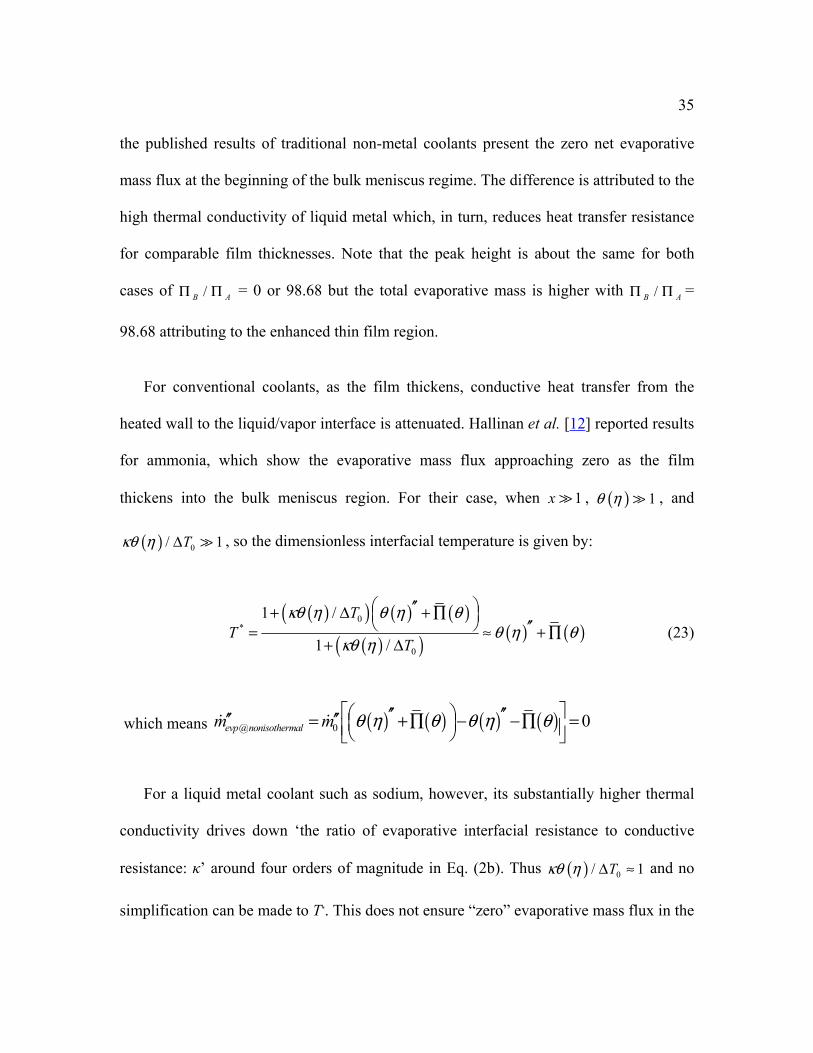
35

the published results of traditional non-metal coolants present the zero net evaporative

mass flux at the beginning of the bulk meniscus regime. The difference is attributed to the

high thermal conductivity of liquid metal which, in turn, reduces heat transfer resistance

for comparable film thicknesses. Note that the peak height is about the same for both

cases of /B AΠ Π = 0 or 98.68 but the total evaporative mass is higher with /B AΠ Π =

98.68 attributing to the enhanced thin film region.

For conventional coolants, as the film thickens, conductive heat transfer from the

heated wall to the liquid/vapor interface is attenuated. Hallinan et al. [12] reported results

for ammonia, which show the evaporative mass flux approaching zero as the film

thickens into the bulk meniscus region. For their case, when 1x , ( ) 1θ η , and

( ) 0/ 1Tκθ η Δ , so the dimensionless interfacial temperature is given by:

( )( ) ( ) ( )

( )( ) ( ) ( )0

*

0

1 /

1 /

TT

T

κθ η θ η θθ η θ

κθ η

′′+ Δ + ∏ ′′= ≈ + ∏

+ Δ (23)

which means ( ) ( ) ( ) ( )@ 0 0evp nonisothermalm m θ η θ θ η θ ′′ ′′′′ ′′= +∏ − −∏ =

For a liquid metal coolant such as sodium, however, its substantially higher thermal

conductivity drives down ‘the ratio of evaporative interfacial resistance to conductive

resistance: κ’ around four orders of magnitude in Eq. (2b). Thus ( ) 0/ 1Tκθ η Δ ≈ and no

simplification can be made to T*. This does not ensure “zero” evaporative mass flux in the

36

bulk meniscus region. We thus observe that the high thermal conductivity of liquid

metals allows evaporative mass flux to occur well into the bulk meniscus.

Another feature of interest from the net evaporative mass flux plot is the evaporation

near the adsorbed film regime. Technically, 0x = should correspond to the adsorbed film

with no evaporation possible. The fact that evaporation does occur at 0x = corresponds

to the choice of boundary conditions in the governing thin film equation Eq. (1). This still

does not explain the variance in initial evaporation fluxes for the different disjoining

pressure cases. The answer here lies in the fact that the net evaporative mass flux, as seen

in Eq. (3), depends in large part upon the second derivative of the film thickness. By

definition, the boundary condition for the curvature was fixed at the far field condition.

The curvature value at 0x = is then not fixed and left to vary with the solution. Hence,

the “initial” net evaporative mass flux at 0x = is seen to vary for the different thin film

solutions.

Figure 5 shows the bulk meniscus solutions for the two extreme cases of ΠB/ΠA= 0

and 98.68. The image depicts the fluid velocity vectors overlaying the surface isotherm

contours of the temperature overheat. The velocity vector field shows that the 1-D

velocity boundary condition at the extended meniscus thin film interface clearly

represents the largest velocity in the model, which indicates that the majority of

evaporation occurs in the extended meniscus thin film region. The temperature overheat

plot shows clear striation, indicating conduction dominant heat transfer, and the presence

37

of evaporation at the meniscus appropriately reduces the overheat towards the capillary

center line.

Figure 6. Column bar charts which compare the extended meniscus thin film and bulk meniscus contributions to capillary meniscus surface area and net evaporative mass flow rate.

0.00E+00

5.00E-12

1.00E-11

1.50E-11

2.00E-11

2.50E-11

3.00E-11

3.50E-11

4.00E-11

Thin Film Bulk Meniscus

ΠB/ΠA= 98.68 ΠB/ΠA= 0

(b) [kg/s]

0.00E+00

5.00E-08

1.00E-07

1.50E-07

2.00E-07

2.50E-07

3.00E-07

Thin Film Bulk Meniscus

ΠB/ΠA= 98.68 ΠB/ΠA= 0

(a) Surface Area [m2]

38

Figure 6 presents column bar charts that compare the meniscus surface area and the

net evaporative mass flow rate for the two extreme cases of thin film disjoining pressures.

The ratio of the bulk meniscus to the thin film meniscus decreases to 21% for the

maximum disjoining pressure (ΠB/ΠA= 98.68) from 38% for the zero disjoining pressure

( 0BΠ = ). The corresponding contributions of the bulk meniscus evaporative flux also

decreased from 17% to 10% when the electronic disjoining component is maximized.

Clearly, appreciable heat and mass transfer takes place in the bulk meniscus region of an

evaporating liquid metal capillary.

The overall trend from these plots is that a larger electronic component of the

disjoining pressure leads towards larger extended meniscus thin film surface area, larger

total capillary meniscus surface area, and larger net evaporative mass flow rate, which

corresponds with larger heat flow rate.

5.2 Comparative study of sodium and lithium coolant

The choice of coolant changes key aspects of a heat pipe such as working temperature

and heat transfer capability. For an alkali metal heat pipe, sodium(Na) and lithium(Li) are

widely considered as proper coolants. However, there is no simple way to conclude

which coolant is proper without studying in further detail. For comparative study, the

characteristics of a sodium coolant heat pipe model are studied in chapter 5.1, and similar

characterization study for a lithium model is needed.

For the case of lithium coolant, the relevant parameters become

39

( )

4.

. @1608

..

.

.

0

( ) 2.9523 (1.5957 10 ) 2.6946(eV)

4.7366(eV)

1 1.2526

0.042851

[N] 5.087565E 12

61.589[ ]

/ 60.93

eV lithium Kelvin

F lithium K

lithuimn lithium

F lithuim

n lithiu

A

m

B

T T

E

E

B

H nm

ϕ

ϕκ

χ κ

−= − × =

=

≈ + =

=

= −

Π

=

=Π

(24)

based on the assumption that the value of the work function(Fig. 7) of lithium has

continuity at melting temperature.

40

Table 3. Fluidic and thermodynamic properties of liquid sodium and lithium at atmospheric pressure[45].

Property Symbol Units Sodium Lithium

Vapor Temperature (1atm) Tv K 1156.1 1608

Molecular Mass M kg⁄mol 0.02299 0.00694

Density ρ kg⁄m3 742.86 400.5

Dynamic Viscosity μ N·s/m2 1.5856E-04 1.6798E-4

Surface Tension γ N⁄m 0.1199 0.2390

Thermal Conductivity λ W/m·K 48.6562 64.9301

Latent Heat of Vaporization hfg KJ⁄kg 3881.5 19763.6

Vapor Pressure Pv MPa 0.10133 0.1112

Electrical Conductivity σ S⁄m 2.54E+06 11.7E+6

41

Figure 7. Temperature-dependence of the Fermi Energy and Work Function of lithium[46].

0

2

4

6

1000 1100 1200 1300 1400 1500 1600

Fermi Energy Work Function

Ene

rgy

Lev

el (

eV)

Temperature (K)

42

Figure 8 presents soulution for total capillary meniscus evaporation in steady status

for both sodium (ΠB/ΠA= 98.68) and lithium (ΠB/ΠA= 60.93). H0 of sodium is 122%

thicker than that of lithium. Starting from a larger thickness ‘H0’, the thin film axial

length of sodium is relatively shorter than that of lithium and connected to the bulk

meniscus at a thicker Htf.sodium (14.2 nm) than Htf.lithium (8.4 nm). The sodium’s shorter and

thicker thin film, however, does not create substantial difference in the area of bulk

meniscus region when compared to lithium, with the main reason being the R >> Htf.

Figure 9 shows contributions of both regions, extended meniscus thin film and bulk

meniscus, to capillary meniscus surface area and net evaporative mass flow rate. The

capillary of lithium has a slightly larger area than that of sodium due to its longer thin

film in fig.9-a. Figure 9-b shows that the evaporative mass flux of lithium is less than that

of sodium under the same overheating condition (ΔT = 0.0005K). The lithium model has

only 51% of total evaporative mass flux to that of the sodium model. However, the

lithium model has 260% greater heat transfer capability due to its hfg being five times

greater than sodium (Lithium: 19763.6 KJ/kg, Sodium: 3881.5 KJ/kg). Overall, the

lithium based heat pipe shows enhanced thin film area and higher heat transfer capability

with less evaporative mass flux under the same overheating condition.

43

Figure 8. Steady total capillary meniscus evaporation solutions of sodium and lithium measured from the adsorption thickness H0 to the capillary centerline

0 50 100 150 200 250 300 3500

50

100

150

200

x (μm)

(b)

Thi

n Fi

lm T

hick

ness

(μm

)

100 105 110 115 120 125 130 135 1400

0.1

0.2

0.3

0.4

0.5

x (μm)

(a)

Thi

n Fi

lm T

hick

ness

(μm

)

Na Thinfilm(ΠB/Π

A=98.68)

Na Meniscus(ΠB/Π

A=98.68)

Li Thinfilm(ΠB/Π

A=60.93)

Li Meniscus(ΠB/Π

A=60.93)

0 50 100 150 200 250 300 3500

1

2

3x 10

−4

x (μm)

(c)

m’ ev

p (kg

/s.m

2 )

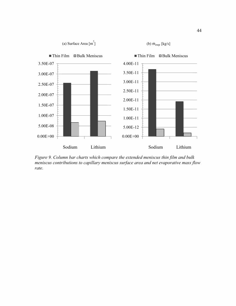
44

Figure 9. Column bar charts which compare the extended meniscus thin film and bulk meniscus contributions to capillary meniscus surface area and net evaporative mass flow rate.

0.00E+00

5.00E-12

1.00E-11

1.50E-11

2.00E-11

2.50E-11

3.00E-11

3.50E-11

4.00E-11

Thin Film Bulk Meniscus

Sodium Lithium

(b) [kg/s]

0.00E+00

5.00E-08

1.00E-07

1.50E-07

2.00E-07

2.50E-07

3.00E-07

3.50E-07

Thin Film Bulk Meniscus

Sodium Lithium

(a) Surface Area [m2]

45

Chapter 6

Results and Discussion

This study effectively models high temperature, liquid metal, extended meniscus

evaporation under non-isothermal interface conditions. The numerical model utilized

correctly incorporates both the full, retarded dispersion force component and the

electronic disjoining pressure component that is unique to liquid metal coolants. The

dispersion force component is calculated using a more thorough and accurate model of

the dielectric permittivity of the liquid sodium coolant. The electronic component is

modeled based on the effective “electron pressure” increase accounting for the

confinement of free electrons in a thin metal film.

When coupled with a CFD model of the evaporating bulk meniscus, the problem as

described above also yields a multiscale numerical model of an evaporating liquid metal

in a capillary tube. The model correctly considers the unique disjoining pressure effects at

the near wall region, including the extended meniscus thin film profile, and captures the

heat and fluid transfer through the bulk meniscus region. The important conceptual

results identified from the present work include the following:

1. Accurate high temperature, liquid metal, capillary evaporation models should

account for both retarded dispersion force and electronic disjoining pressures in

the extended meniscus thin film regime.

2. Integration of the evaporative mass flux across the total meniscus surface area

produces total capillary evaporative mass flow and heat transfer rates.

46

3. Unlike more traditional or non-metallic coolants, evaporative mass and heat flow

occurs in the bulk meniscus region of evaporating micro-capillaries.

4. The clear trend from these comparisons is that a larger electronic component of

the disjoining pressure leads towards larger extended meniscus thin film surface

area, larger total capillary meniscus surface area, and larger net evaporative mass

flow rate with larger heat flow rate.

5. The lithium based heat pipe shows enhanced thin film area and higher heat

transfer capability with less evaporative mass flux than sodium based one under

the same overheating condition.

47

List of References

48

1. Cao, Y., A. Faghri, and E.T. Mahefkey, Micro/miniature heat pipes and operating limitations. ASME-PUBLICATIONS-HTD, 1993. 236: p. 55-55.

2. Ku, J., Overview of capillary pumped loop technology. ASME-PUBLICATIONS-HTD, 1993. 236: p. 1-1.

3. Anderson, W.G., High Temperature Capillary Pumped Loops. ASME-PUBLICATIONS-HTD, 1993. 236: p. 93-93.

4. Khrustalev, D. and A. Faghri, Thermal analysis of a micro heat pipe. Journal of Heat Transfer, 1994. 116(1): p. 189-198.

5. Wayner Jr, P.C., Intermolecular forces in phase‐change heat transfer: 1998 Kern award review. AIChE journal, 1999. 45(10): p. 2055-2068.

6. Derjaguin, B., L. Leonov, and V. Roldughin, Disjoining pressure in liquid metallic films. Journal of Colloid and Interface Science, 1985. 108(1): p. 207-214.

7. Wayner Jr, P. and J. Schonberg. Heat transfer and fluid flow in an evaporating extended meniscus. 1990.

8. Derjaguin, B., S. Nerpin, and N. Churaev, Effect of film transfer upon evaporation of liquids from capillaries. Bulletin Rilem, 1965. 29: p. 93-98.

9. Schrage, R.W., A theoretical study of interphase mass transfer1953: Columbia University Press New York.

10. Potash Jr, M. and P. Wayner Jr, Evaporation from a two-dimensional extended meniscus. International Journal of Heat and Mass Transfer, 1972. 15(10): p. 1851-1863.

11. Wayner Jr, P., Y. Kao, and L. LaCroix, The interline heat-transfer coefficient of an evaporating wetting film. International Journal of Heat and Mass Transfer, 1976. 19(5): p. 487-492.

12. Hallinan, K., et al., Evaporation from an extended meniscus for nonisothermal interfacial conditions. Journal of thermophysics and heat transfer, 1994. 8: p. 709-716.

13. Dzyaloshinskii, I., E. Lifshitz, and L.P. Pitaevskii, GENERAL THEORY OF VAN DER WAALS'FORCES. Physics-Uspekhi, 1961. 4(2): p. 153-176.

14. Moosman, S. and G. Homsy, Evaporating menisci of wetting fluids. Journal of Colloid and Interface Science, 1980. 73(1): p. 212-223.

15. Truong, J.G. and P.C. Wayner Jr, Effects of capillary and van der Waals dispersion forces on the equilibrium profile of a wetting liquid: Theory and experiment. The Journal of Chemical Physics, 1987. 87: p. 4180.

16. DasGupta, S., J. Schonberg, and P. Wayner, Investigation of an evaporating extended meniscus based on the augmented Young-Laplace equation. TRANSACTIONS-AMERICAN SOCIETY OF MECHANICAL ENGINEERS JOURNAL OF HEAT TRANSFER, 1993. 115: p. 201-201.

17. Derjaguin, B. and V. Roldughin, Influence of the ambient medium on the disjoining pressure of liquid metallic films. Surface Science, 1985. 159(1): p. 69-82.

18. Roldughin, V.I., Quantum-size colloid metal systems. Russian Chemical Reviews, 2000. 69: p. 821.

49

19. Ajaev, V.S. and D.A. Willis, Thermocapillary flow and rupture in films of molten metal on a substrate. Physics of Fluids, 2003. 15: p. 3144.

20. Ajaev, V.S. and D.A. Willis, Heat transfer, phase change, and thermocapillary flow in films of molten metal on a substrate. Numerical Heat Transfer, 2006. 50(4): p. 301-313.

21. Tipton Jr, J.B., K.D. Kihm, and D.M. Pratt, Modeling Alkaline Liquid Metal (Na) Evaporating Thin Films Using Both Retarded Dispersion and Electronic Force Components. Journal of Heat Transfer, 2009. 131: p. 121015.

22. Swanson, L. and G. Herdt, Model of the evaporating meniscus in a capillary tube. Journal of Heat Transfer (Transactions of the ASME (American Society of Mechanical Engineers), Series C);(United States), 1992. 114(2).

23. Chebaro, H., et al., Evaporation from a porous wick heat pipe for isothermal interfacial conditions. ASME-PUBLICATIONS-HTD, 1993. 221: p. 23-23.

24. Stephan, P. and C. Busse, Analysis of the heat transfer coefficient of grooved heat pipe evaporator walls. International Journal of Heat and Mass Transfer, 1992. 35(2): p. 383-391.

25. Schonberg, J., S. DasGupta, and P. Wayner, An augmented Young-Laplace model of an evaporating meniscus in a microchannel with high heat flux. Experimental thermal and fluid science, 1995. 10(2): p. 163-170.

26. Khrustalev, D. and A. Faghri, Heat transfer during evaporation on capillary-grooved structures of heat pipes. Journal of Heat Transfer, 1995. 117: p. 740.

27. Khrustalev, D. and A. Faghri, Fluid flow effects in evaporation from liquid–vapor meniscus. Journal of Heat Transfer, 1996. 118: p. 725.

28. Kim, H., Temperature and Velocity Field Mappings for Micro-scale Heat and Mass Transport Phenomena, 2001, Texas A & M University.

29. Yan, J., L. Qiu-Sheng, and L. Rong, Coupling of evaporation and thermocapillary convection in a liquid layer with mass and heat exchanging interface. Chinese Physics Letters, 2008. 25: p. 608.

30. Chebaro, H. and K. Hallinan, Boundary conditions for an evaporating thin film for isothermal interfacial conditions. Journal of Heat Transfer, 1993. 115(3): p. 816-819.

31. Drude, P., The theory of optics1922: Longmans, Green. 32. Bennett, H. and J. Bennett, Validity of the Drude theory for silver, gold and

aluminum in the infrared. Optical Properties and Electronic Structure of Metals and Alloys, edited by F. Abeles (North Holland, Amsterdam, 1966), 1966: p. 175 - 195.

33. Hodgson, J.N., The optical properties of liquid metals, in Liquid Metals—Chemistry and Physics, S.Z. Beer, Editor 1972, Marcel Dekker: New York. p. 331-371.

34. Inagaki, T., et al., Optical properties of liquid Na between 0.6 and 3.8 eV. Physical Review B, 1976. 13(12): p. 5610.

35. March, N. and B. Paranjape, Mean free path effects in the dielectric function of a liquid metal. Physics and Chemistry of Liquids an International Journal, 1987. 17(1): p. 55-71.

50

36. Shimoji, M., Liquid metals: an introduction to the physics and chemistry of metals in the liquid state. Vol. 266. 1977: Academic Press.

37. Takens, W., et al., A spectroscopic study of free evaporation of sodium. Rarefied Gas Dynamics, 1984: p. 967–974.

38. Wilson, J., The structure of liquid metals and alloys. Metallurgical Reviews, 1965. 10(1): p. 381-590.

39. Fink, J. and L. Leibowitz, A consistent assessment of the thermophysical properties of sodium. High temperature and materials science, 1996. 35(1): p. 65-103.

40. Landau, L.D. and E.M. Lifshits, The electrodynamics of continuous media. Moscow Izdatel Nauka Teoreticheskaia Fizika, 1982. 8: p. 624.

41. Coutts, T.J., Electrical conduction in thin metal films1974: Elsevier. 42. Alchagirov, B.B., R.K. Arkhestov, and K.B. Khokonov, Temperature

Dependence of the Electron Work Function of Solid and Liquid Sodium. Russian Journal of Physical Chemistry, 1993. 67(9): p. 1892 - 1895.

43. Cammenga, H.K., Evaporation mechanisms of liquids. Current topics in materials science, 1980. 5: p. 335-446.

44. Tipton Jr, J.B., Unique Characteristics of Liquid Metal Extended Meniscus Evaporation. 2009.

45. Jeppson, D., et al., Lithium literature review: lithium's properties and interactions, 1978, Hanford Engineering Development Lab., Richland, Wash.(USA).

46. Wong, K., G. Tikhonov, and V.V. Kresin, Temperature-dependent work functions of free alkali-metal nanoparticles. Physical Review B, 2002. 66(12): p. 125401.

51

Vita

Hunju Yi was born in Asan, South Korea, to the parents of Eunkwang Yi and Chunhee Park. He attended West Daejeon high school and completed his undergraduate course in aerospace engineering at Chungnam national university in Daejeon, South Korea.

He moved to the United States and was accepted at the University of Tennessee, Knoxville. He graduated with a Master of Science degree in Mechanical Engineering under the advising of Dr. Kenneth D. Kihm at MINSFET.